Landslide-Induced Damage Probability Estimation Coupling InSAR and Field Survey Data by Fragility Curves

 , ,
, ,  ,
,
Abstract
:
1. Introduction
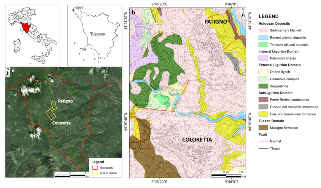
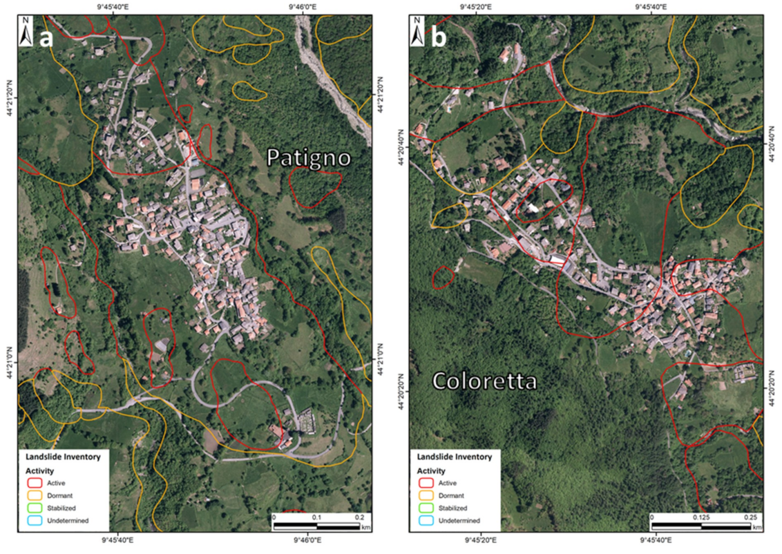
2. Study Area
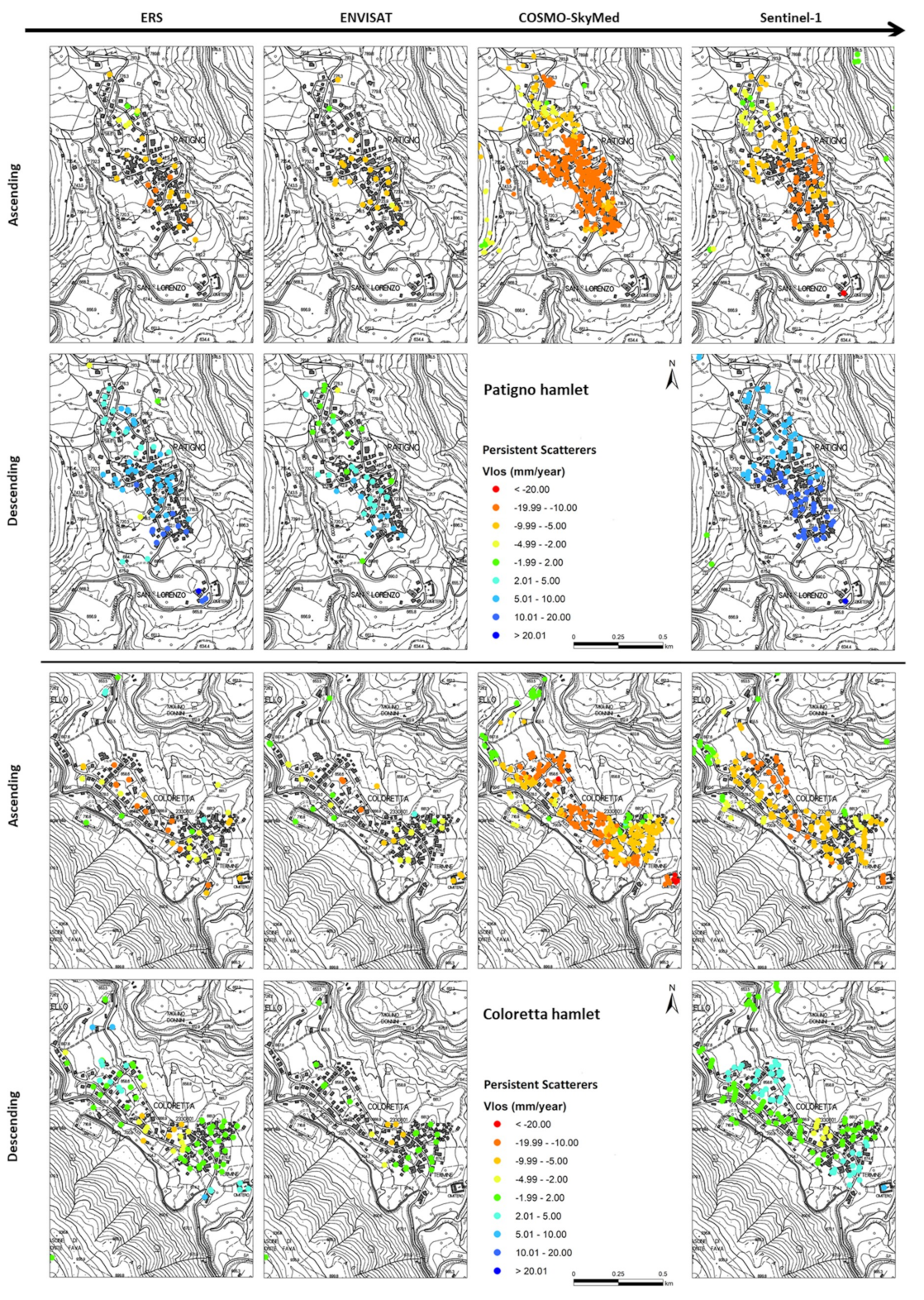
Satellite Velocity Maps
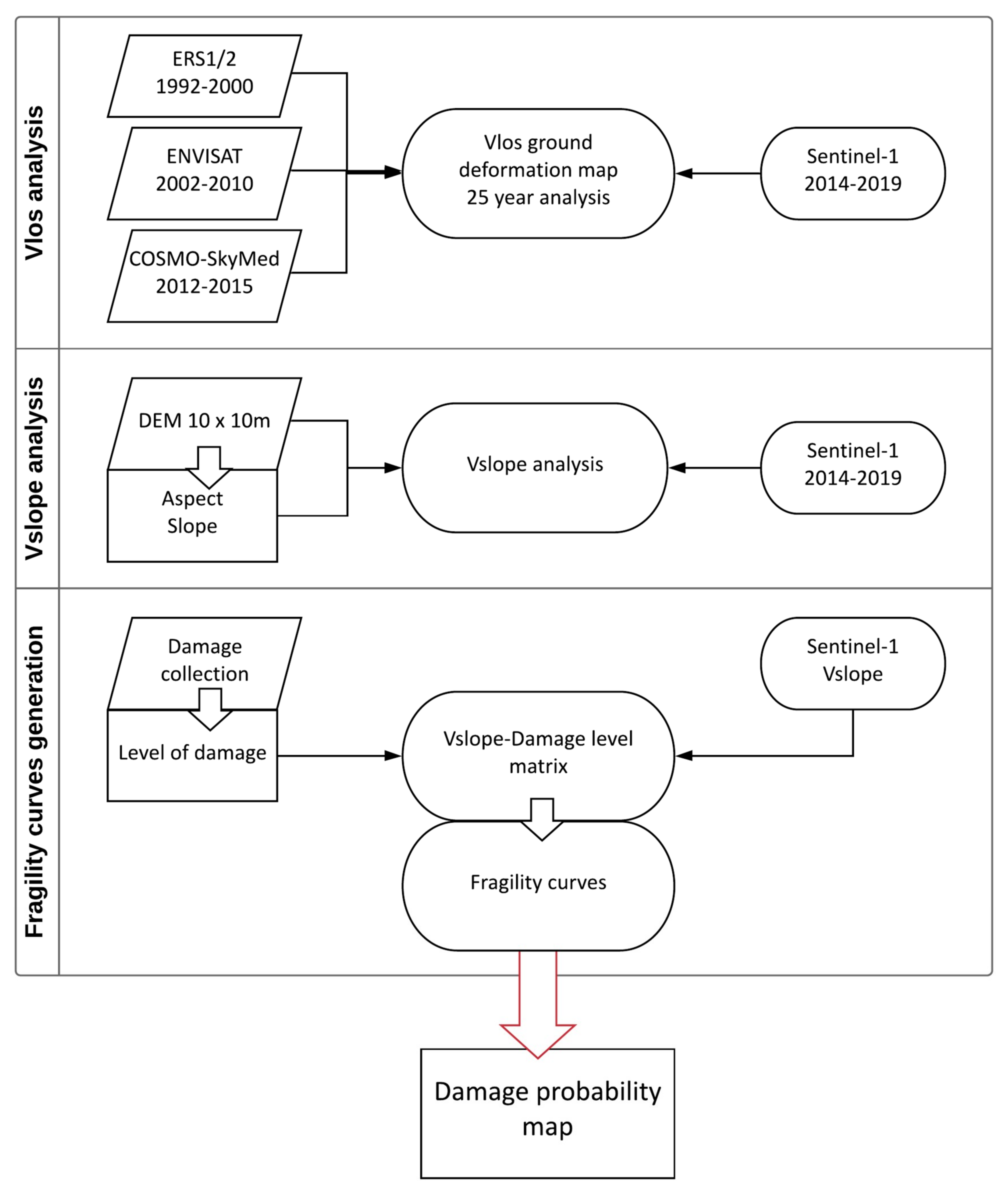
3. Methodology
3.1. Velocity Along the Slope
3.2. Damage Classification
3.3. Evaluation and Validation of the Relationship between Vslope Values and Assessed Damage
- -
- LOW—o damage and negligible;
- -
- MEDIUM—weak and moderate;
- -
- SEVERE—severe and very severe;
- -
- HIGH—potential collapse and unusable.
- -
- ND both parameters—no Vslope velocity and damage information;
- -
- ND one parameter—no Vslope velocity or damage information;
- -
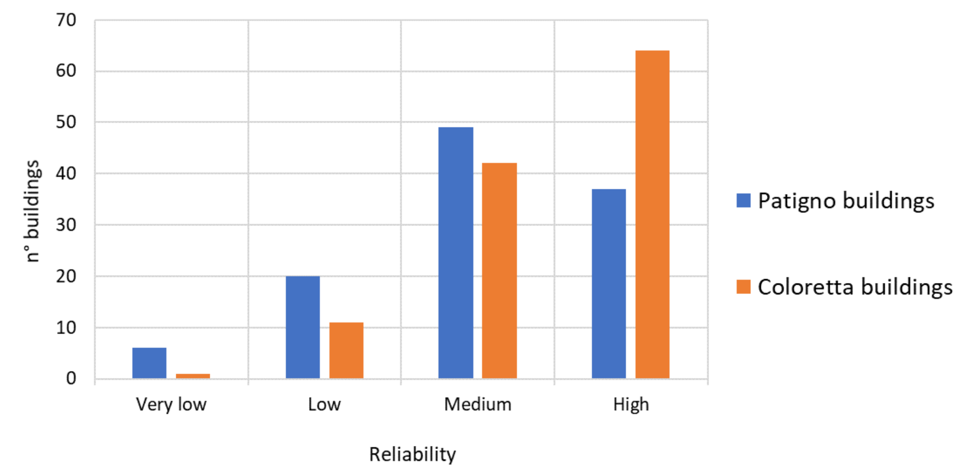
- Very low reliability—STABILITY range of Vslope velocities combined with HIGH level of damage or HIGH Vslope velocity combined with LOW level of damage;
- -
- Low reliability—STABILITY range or LOW Vslope velocities combined with SEVERE or HIGH level of damage, respectively, or MEDIUM or HIGH Vslope velocity combined with LOW or MEDIUM level of damage, respectively;
- -
- Medium reliability—STABILITY range, LOW or MEDIUM Vslope velocities combined with MEDIUM, SEVERE or HIGH level of damage, respectively, or LOW, MEDIUM or HIGH Vslope velocity combined with LOW, MEDIUM or SEVERE level of damage, respectively;
- -
- High reliability—only for good correspondence, i.e., STABILITY range of Vslope velocity combined with LOW level of damage, LOW Vslope velocity combined with MEDIUM level of damage, MEDIUM Vslope velocity combined with SEVERE level of damage and HIGH Vslope velocity combined with HIGH level of damage.
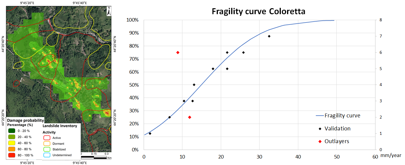
3.4. Fragility Curves and Damage Probability Map
4. Results
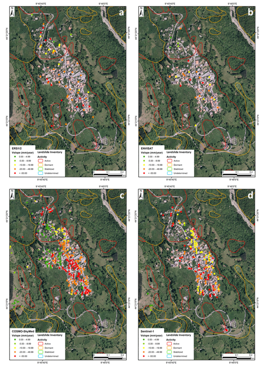
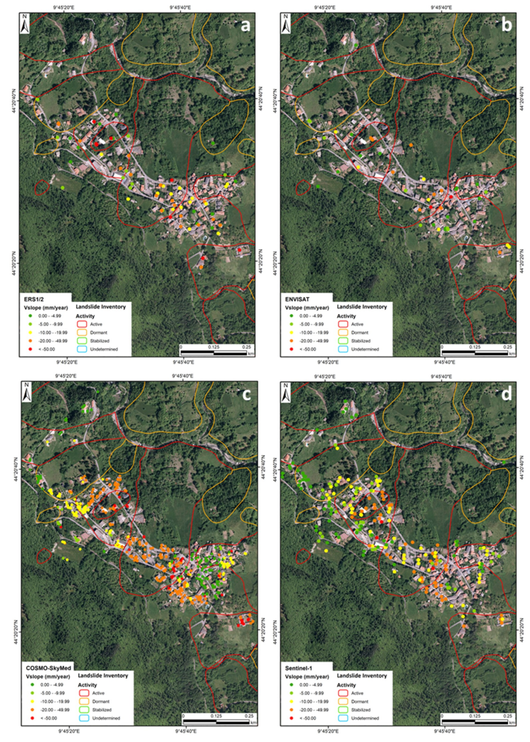
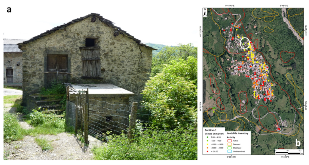
4.1. Vslope Deformation Maps
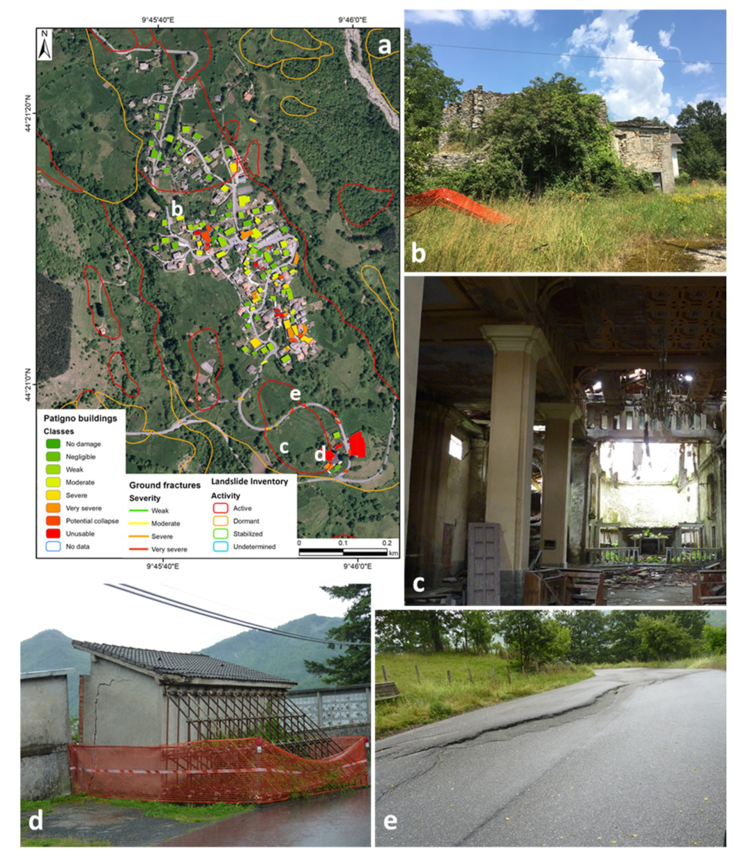
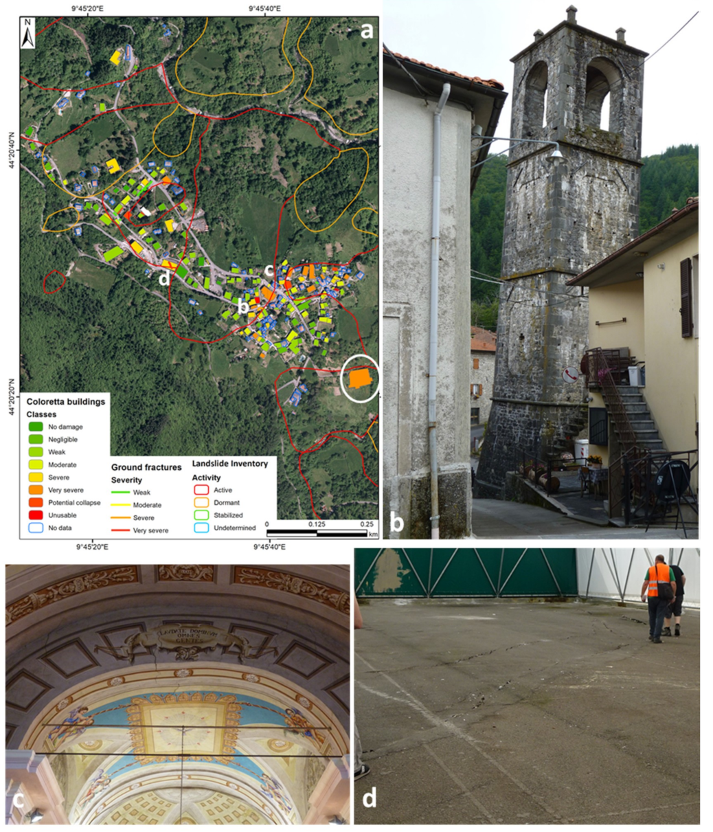
4.2. Building Damage Classification Maps
4.3. Vslope-Damage Assessment
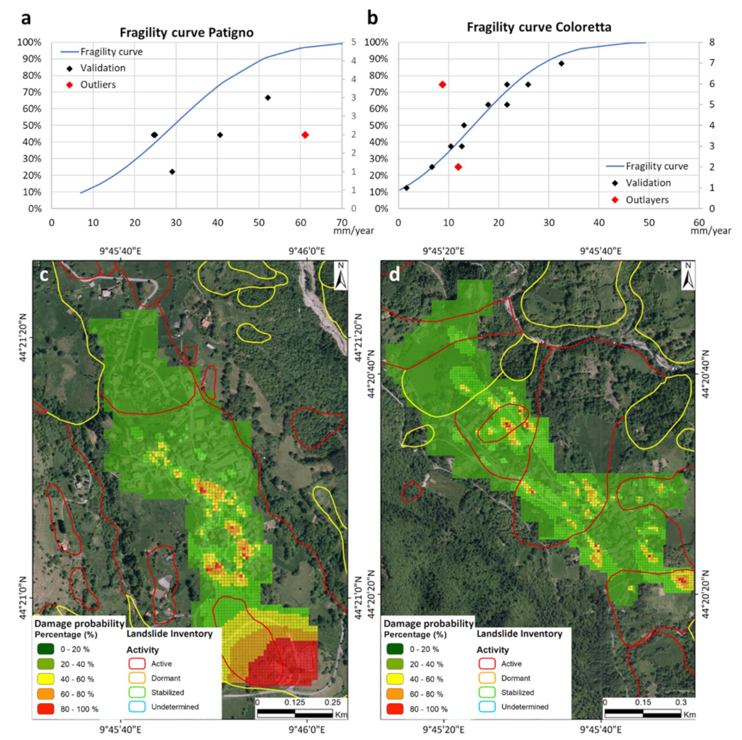
4.4. Landslide-Induced Damage Probability Maps
- -
- the northern portion of the hamlet with no or very low probability of damage (0–20%);
- -
- the central portion where the probability shows different values localized areas with high probability of damage within a general low rate;
- -
- the southern with generally high values of probability of damage (60–100%).
5. Discussions
- -
- buildings abandoned that can be classified rightly as un-inhabitable (higher class of damage) but can be in a stable area. In this case, the correlation between the damage level and the Vslope velocity classes results very low (Figure 11) due to the intensity of the fractures and cracks;
- -
- new or restored constructions that show no cracks or negligible damage, that can be located in areas with recorded medium or high velocities. Even if high Vslope velocities are registered, these are not sufficient to have sudden visible consequences on new or restored structures. In these cases, the correlation between the damage and the Vslope classes results in very low to low.
- -
- they do not consider the different load-bearing structure of the buildings; this factor is expeditiously evaluated only during the damage level survey;
- -
- the damage classification is referred to the full life of the buildings that, generally, is different with respect to the monitored period;
- -
- the activity, direction, number of the landslides affecting the area of interest, as well as their typology (e.g., rotational, sliding, etc.)
- -
- considering the C-band resolution for each building, it is sometimes not possible to have more than one or two PSs for building. For this reason, differential motions for single buildings were not easily detected.
6. Conclusions
Supplementary Materials
Author Contributions
Funding
Acknowledgments
Conflicts of Interest
References
- Herrera, G.; Mateos, R.M.; García-Davalillo, J.C.; Grandjean, G.; Poyiadji, E.; Maftei, R.; Filipciuc, T.-C.; Auflič, M.J.; Jež, J.; Podolszki, L. Landslide databases in the Geological Surveys of Europe. Landslides 2018, 15, 359–379. [Google Scholar] [CrossRef]
- Bogaard, T.A.; Greco, R. Landslide hydrology: From hydrology to pore pressure. Wiley Interdiscip. Rev. Water 2016, 3, 439–459. [Google Scholar] [CrossRef]
- Tanyaş, H.; van Westen, C.J.; Allstadt, K.E.; Jibson, R.W. Factors controlling landslide frequency–area distributions. Earth Surf. Process. Landf. 2019, 44, 900–917. [Google Scholar] [CrossRef]
- Gariano, S.L.; Guzzetti, F. Landslides in a changing climate. Earth-Sci. Rev. 2016, 162, 227–252. [Google Scholar] [CrossRef] [Green Version]
- Segoni, S.; Piciullo, L.; Gariano, S.L. A review of the recent literature on rainfall thresholds for landslide occurrence. Landslides 2018, 15, 1483–1501. [Google Scholar] [CrossRef]
- Jaboyedoff, M.; Michoud, C.; Derron, M.-H.; Voumard, J.; Leibundgut, G.; Sudmeier-Rieux, K.; Nadim, F.; Leroi, E. Human-induced landslides: Toward the analysis of anthropogenic changes of the slope environment. In Landslides and Engineered Slopes. Experience, Theory and Practice; CRC Press: Boca Raton, FL, USA, 2018; pp. 217–232. [Google Scholar]
- Godt, J.; Coe, J.; Savage, W. Relation between cost of damaging landslides and construction age, Alameda County, California, USA, El Niño winter storm season, 1997–1998. In Proceedings of the 8th International Symposium on Landslides, Cardiff, Wales, 26–30 June 2000; pp. 26–30. [Google Scholar]
- Schuster, R.L.; Fleming, R.W. Economic losses and fatalities due to landslides. Bull. Assoc. Eng. Geol. 1986, 23, 11–28. [Google Scholar] [CrossRef]
- Schuster, R.L. Socioeconomic significance of landslides. Landslides: Investigation and Mitigation; Transportation Research Board Special Report; National Academy Press: Washington, DC, USA, 1996; Volume 247, pp. 12–35. [Google Scholar]
- Haque, U.; Blum, P.; Da Silva, P.F.; Andersen, P.; Pilz, J.; Chalov, S.R.; Malet, J.-P.; Auflič, M.J.; Andres, N.; Poyiadji, E. Fatal landslides in Europe. Landslides 2016, 13, 1545–1554. [Google Scholar] [CrossRef]
- Moore, R.; McInnes, R. The impacts of landslides on global society: Planning for change. Landslides and engineered slopes: Experience, theory and practice. In Proceedings of the 12th International Symposium on Landslides, Napoli, Italy, 12–19 June 2016; pp. 1461–1468. [Google Scholar]
- Petley, D. Global patterns of loss of life from landslides. Geology 2012, 40, 927–930. [Google Scholar] [CrossRef]
- Goetz, J.N.; Guthrie, R.H.; Brenning, A. Integrating physical and empirical landslide susceptibility models using generalized additive models. Geomorphology 2011, 129, 376–386. [Google Scholar] [CrossRef]
- Gullà, G.; Peduto, D.; Borrelli, L.; Antronico, L.; Fornaro, G. Geometric and kinematic characterization of landslides affecting urban areas: The Lungro case study (Calabria, Southern Italy). Landslides 2017, 14, 171–188. [Google Scholar] [CrossRef]
- Guzzetti, F.; Mondini, A.C.; Cardinali, M.; Fiorucci, F.; Santangelo, M.; Chang, K.-T. Landslide inventory maps: New tools for an old problem. Earth-Sci. Rev. 2012, 112, 42–66. [Google Scholar] [CrossRef] [Green Version]
- Van Westen, C.J. Remote sensing and GIS for natural hazards assessment and disaster risk management. Treatise Geomorphol. 2013, 3, 259–298. [Google Scholar]
- Corominas, J.; Moya, J.; Lloret, A.; Gili, J.; Angeli, M.; Pasuto, A.; Silvano, S. Measurement of landslide displacements using a wire extensometer. Eng. Geol. 2000, 55, 149–166. [Google Scholar] [CrossRef]
- Zhang, Y.; Tang, H.; Li, C.; Lu, G.; Cai, Y.; Zhang, J.; Tan, F. Design and testing of a flexible inclinometer probe for model tests of landslide deep displacement measurement. Sensors 2018, 18, 224. [Google Scholar] [CrossRef] [PubMed]
- Li, Y.; Huang, J.; Jiang, S.-H.; Huang, F.; Chang, Z. A web-based GPS system for displacement monitoring and failure mechanism analysis of reservoir landslide. Sci. Rep. 2017, 7, 17171. [Google Scholar] [CrossRef] [PubMed]
- Colesanti, C.; Ferretti, A.; Prati, C.; Rocca, F. Monitoring landslides and tectonic motions with the Permanent Scatterers Technique. Eng. Geol. 2003, 68, 3–14. [Google Scholar] [CrossRef]
- Cotecchia, V.; Grassi, D.; Merenda, L. Fragilità dell’area urbana occidentale di Ancona dovuta a movimenti di massa profondi e superficiali ripetutisi nel 1982. Geol. Appl. Idrogeol. 1995, 30, 633–657. [Google Scholar]
- Glenn, N.F.; Streutker, D.R.; Chadwick, D.J.; Thackray, G.D.; Dorsch, S.J. Analysis of LiDAR-derived topographic information for characterizing and differentiating landslide morphology and activity. Geomorphology 2006, 73, 131–148. [Google Scholar] [CrossRef]
- Jaboyedoff, M.; Oppikofer, T.; Abellán, A.; Derron, M.-H.; Loye, A.; Metzger, R.; Pedrazzini, A. Use of LIDAR in landslide investigations: A review. Nat. Hazards 2012, 61, 5–28. [Google Scholar] [CrossRef]
- Bovenga, F.; Wasowski, J.; Nitti, D.; Nutricato, R.; Chiaradia, M. Using COSMO/SkyMed X-band and ENVISAT C-band SAR interferometry for landslides analysis. Remote Sens. Environ. 2012, 119, 272–285. [Google Scholar] [CrossRef]
- Crosetto, M.; Monserrat, O.; Cuevas-González, M.; Devanthéry, N.; Crippa, B. Persistent scatterer interferometry: A review. ISPRS J. Photogramm. Remote Sens. 2016, 115, 78–89. [Google Scholar] [CrossRef]
- Del Soldato, M.; Riquelme, A.; Bianchini, S.; Tomàs, R.; Di Martire, D.; De Vita, P.; Moretti, S.; Calcaterra, D. Multisource data integration to investigate one century of evolution for the Agnone landslide (Molise, southern Italy). Landslides 2018, 15, 2113–2128. [Google Scholar] [CrossRef] [Green Version]
- Tofani, V.; Raspini, F.; Catani, F.; Casagli, N. Persistent Scatterer Interferometry (PSI) technique for landslide characterization and monitoring. Remote Sens. 2013, 5, 1045–1065. [Google Scholar] [CrossRef]
- Bianchini, S.; Raspini, F.; Solari, L.; Del Soldato, M.; Ciampalini, A.; Rosi, A.; Casagli, N. From Picture to Movie: Twenty Years of Ground Deformation recording over Tuscany Region (Italy) with Satellite InSAR. Front. Earth Sci. 2018, 6, 177. [Google Scholar] [CrossRef]
- Tomás, R.; Li, Z. Earth Observations for Geohazards: Present and Future Challenges; Multidisciplinary Digital Publishing Institute: Basel, Switzerland, 2017. [Google Scholar]
- Del Soldato, M.; Farolfi, G.; Rosi, A.; Raspini, F.; Casagli, N. Subsidence Evolution of the Firenze–Prato–Pistoia Plain (Central Italy) Combining PSI and GNSS Data. Remote Sens. 2018, 10, 1146. [Google Scholar] [CrossRef]
- Nobile, A.; Dille, A.; Monsieurs, E.; Basimike, J.; Bibentyo, T.; d’Oreye, N.; Kervyn, F.; Dewitte, O. Multi-temporal DInSAR to characterise landslide ground deformations in a tropical urban environment: Focus on Bukavu (DR Congo). Remote Sens. 2018, 10, 626. [Google Scholar] [CrossRef]
- Novellino, A.; Cigna, F.; Sowter, A.; Ramondini, M.; Calcaterra, D. Exploitation of the Intermittent SBAS (ISBAS) algorithm with COSMO-SkyMed data for landslide inventory mapping in north-western Sicily, Italy. Geomorphology 2017, 280, 153–166. [Google Scholar] [CrossRef]
- Bardi, F.; Raspini, F.; Frodella, W.; Lombardi, L.; Nocentini, M.; Gigli, G.; Morelli, S.; Corsini, A.; Casagli, N. Monitoring the rapid-moving reactivation of Earth flows by means of GB-InSAR: The April 2013 Capriglio Landslide (Northern Appennines, Italy). Remote Sens. 2017, 9, 165. [Google Scholar] [CrossRef]
- Del Soldato, M.; Riquelme, A.; Tomás, R.; De Vita, P.; Moretti, S. Application of structure from motion photogrammetry to multi-temporal geomorphological analyses: Case studies from Italy and Spain. Geogr. Fis. E Din. Quat. 2018, 41, 51–66. [Google Scholar]
- Fiorucci, F.; Giordan, D.; Santangelo, M.; Dutto, F.; Rossi, M.; Guzzetti, F. Criteria for the optimal selection of remote sensing optical images to map event landslides. Nat. Hazards Earth Syst. Sci. 2018, 18, 405–417. [Google Scholar] [CrossRef] [Green Version]
- Stumpf, A.; Malet, J.-P.; Delacourt, C. Correlation of satellite image time-series for the detection and monitoring of slow-moving landslides. Remote Sens. Environ. 2017, 189, 40–55. [Google Scholar] [CrossRef]
- Casagli, N.; Frodella, W.; Morelli, S.; Tofani, V.; Ciampalini, A.; Intrieri, E.; Raspini, F.; Rossi, G.; Tanteri, L.; Lu, P. Spaceborne, UAV and ground-based remote sensing techniques for landslide mapping, monitoring and early warning. Geoenviron. Disasters 2017, 4, 9. [Google Scholar] [CrossRef]
- Rossi, G.; Tanteri, L.; Tofani, V.; Vannocci, P.; Moretti, S.; Casagli, N. Multitemporal UAV surveys for landslide mapping and characterization. Landslides 2018, 1–8. [Google Scholar] [CrossRef]
- Turner, D.; Lucieer, A.; de Jong, S. Time series analysis of landslide dynamics using an unmanned aerial vehicle (UAV). Remote Sens. 2015, 7, 1736–1757. [Google Scholar] [CrossRef]
- Tomás, R.; Romero, R.; Mulas, J.; Marturià, J.J.; Mallorquí, J.J.; López-Sánchez, J.M.; Herrera, G.; Gutiérrez, F.; González, P.J.; Fernández, J. Radar interferometry techniques for the study of ground subsidence phenomena: A review of practical issues through cases in Spain. Environ. Earth Sci. 2014, 71, 163–181. [Google Scholar] [CrossRef]
- Crosetto, M.; Biescas, E.; Duro, J.; Closa, J.; Arnaud, A. Generation of advanced ERS and Envisat interferometric SAR products using the stable point network technique. Photogramm. Eng. Remote Sens. 2008, 74, 443–450. [Google Scholar] [CrossRef]
- Joyce, K.; Samsonov, S.; Levick, S.R.; Engelbrecht, J.; Belliss, S. Mapping and monitoring geological hazards using optical, LiDAR, and synthetic aperture RADAR image data. Nat. Hazards 2014, 73, 137–163. [Google Scholar] [CrossRef]
- Solari, L.; Raspini, F.; Del Soldato, M.; Bianchini, S.; Ciampalini, A.; Ferrigno, F.; Tucci, S.; Casagli, N. Satellite radar data for back-analyzing a landslide event: The Ponzano (Central Italy) case study. Landslides 2018, 15, 773–782. [Google Scholar] [CrossRef]
- Corominas, J.; van Westen, C.; Frattini, P.; Cascini, L.; Malet, J.-P.; Fotopoulou, S.; Catani, F.; Van Den Eeckhaut, M.; Mavrouli, O.; Agliardi, F. Recommendations for the quantitative analysis of landslide risk. Bull. Eng. Geol. Environ. 2014, 73, 209–263. [Google Scholar] [CrossRef]
- Geudtner, D.; Torres, R.; Snoeij, P.; Davidson, M.; Rommen, B. Sentinel-1 System capabilities and applications. In Proceedings of the IGARSS, Munich, Germany, 22–27 June 2012; pp. 1457–1460. [Google Scholar]
- Torres, R.; Snoeij, P.; Geudtner, D.; Bibby, D.; Davidson, M.; Attema, E.; Potin, P.; Rommen, B.; Floury, N.; Brown, M. GMES Sentinel-1 mission. Remote Sens. Environ. 2012, 120, 9–24. [Google Scholar] [CrossRef]
- Rybár, J. Increasing impact of anthropogenic activities upon natural slope stability. In Proceedings of the International Symposium on Engineering Geology and the Environment, Athens, Greece, 23–27 June 1997; pp. 23–27. [Google Scholar]
- Chiocchio, C.; Iovine, G.; Parise, M. A proposal for surveying and classifying landslide damage to buildings in urban areas. Processing of the International Symposium on Engineering Geology and the Environment, Athens, Greece, 23–27 June 1997. [Google Scholar]
- Alexander, D. Landslide damage to buildings. Environ. Geol. Water Sci. 1986, 8, 147–151. [Google Scholar] [CrossRef]
- Fotopoulou, S.; Pitilakis, K. Fragility curves for reinforced concrete buildings to seismically triggered slow-moving slides. Soil Dyn. Earthq. Eng. 2013, 48, 143–161. [Google Scholar] [CrossRef]
- Mavrouli, O.; Fotopoulou, S.; Pitilakis, K.; Zuccaro, G.; Corominas, J.; Santo, A.; Cacace, F.; De Gregorio, D.; Di Crescenzo, G.; Foerster, E. Vulnerability assessment for reinforced concrete buildings exposed to landslides. Bull. Eng. Geol. Environ. 2014, 73, 265–289. [Google Scholar] [CrossRef]
- Negulescu, C.; Foerster, E. Parametric studies and quantitative assessment of the vulnerability of a RC frame building exposed to differential settlements. Nat. Hazards Earth Syst. Sci. 2010, 10, 1781–1792. [Google Scholar] [CrossRef] [Green Version]
- Negulescu, C.; Ulrich, T.; Baills, A.; Seyedi, D. Fragility curves for masonry structures submitted to permanent ground displacements and earthquakes. Nat. Hazards 2014, 74, 1461–1474. [Google Scholar] [CrossRef]
- Peduto, D.; Ferlisi, S.; Nicodemo, G.; Reale, D.; Pisciotta, G.; Gullà, G. Empirical fragility and vulnerability curves for buildings exposed to slow-moving landslides at medium and large scales. Landslides 2017, 14, 1993–2007. [Google Scholar] [CrossRef]
- Peduto, D.; Nicodemo, G.; Maccabiani, J.; Ferlisi, S. Multi-scale analysis of settlement-induced building damage using damage surveys and DInSAR data: A case study in The Netherlands. Eng. Geol. 2017, 218, 117–133. [Google Scholar] [CrossRef]
- Saeidi, A.; Deck, O.; Verdel, T. Development of building vulnerability functions in subsidence regions from empirical methods. Eng. Struct. 2009, 31, 2275–2286. [Google Scholar] [CrossRef] [Green Version]
- Peel, M.C.; Finlayson, B.L.; McMahon, T.A. Updated world map of the Köppen-Geiger climate classification. Hydrol. Earth Syst. Sci. Discuss. 2007, 4, 439–473. [Google Scholar] [CrossRef]
- Feroni, A.C.; Leoni, L.; Martelli, L.; Martinelli, P.; Ottria, G.; Sarti, G. The Romagna Apennines, Italy: An eroded duplex. Geol. J. 2001, 36, 39–54. [Google Scholar] [CrossRef]
- Elter, P.; Schwab, K. Nota illustrativa della carta geologica all’1: 50.000 della zona di Carro-Zeri-Pontremoli. Boll. Soc. Geol. Ital 1959, 78, 157–188. [Google Scholar]
- Federici, P.; Puccinelli, A.; Chelli, A.; D’Amato Avanzi, G.; Ribolini, A.; Verani, M. La grande frana di Patigno di Zeri (Massa-Carrara). Mem. Della Accad. Lunigianese Di Sci. Giovanni Capellini. Sci. Nat. Fis. E Mat. 2000, 70, 3–51. [Google Scholar]
- Chelli, A.; Stefanini, M.C. Geomorphological Features and Temporal Distribution of the Present-day Landslides Activity in the High Gordana Basin (Zeri, Northern Apennines): A Dendrogeomorphological Anlysis. Comitato Glaciologico Italiano 1999, 22, 105–114. [Google Scholar]
- Baldi, P.; Cenni, N.; Fabris, M.; Zanutta, A. Kinematics of a landslide derived from archival photogrammetry and GPS data. Geomorphology 2008, 102, 435–444. [Google Scholar] [CrossRef]
- Raiti, R.; Signanini, P.; Torrese, P.; Sammartino, P. II metodo della ricollocazione nella risoluzione di problematiche geologicoambientali: Il caso di Zeri (Massa-Carrara). G. Di Geol. Appl. 2006, 3, 213–220. [Google Scholar]
- Portale Cartografico Nazionale (PCN) of the Italian Ministry for the Environment, Territory and Sea (METS). Available online: http://www.pcn.minambiente.it/ (accessed on 15 May 2019).
- Interferometric SAR satellite website of the Region of Tuscany. Available online: https://geoportale.lamma.rete.toscana.it/difesa_suolo/ (accessed on 15 May 2019).
- Ferretti, A.; Prati, C.; Rocca, F. Permanent scatterers in SAR interferometry. Geosci. Remote Sens. IEEE Trans. 2001, 39, 8–20. [Google Scholar] [CrossRef]
- Ferretti, A.; Prati, C.; Rocca, F. Nonlinear subsidence rate estimation using permanent scatterers in differential SAR interferometry. IEEE Trans. Geosci. Remote Sens. 2000, 38, 2202–2212. [Google Scholar] [CrossRef] [Green Version]
- Costantini, M.; Falco, S.; Malvarosa, F.; Minati, F.; Trillo, F.; Vecchioli, F. Persistent scatterer pair interferometry: Approach and application to COSMO-SkyMed SAR data. IEEE J. Sel. Top. Appl. Earth Obs. Remote Sens. 2014, 7, 2869–2879. [Google Scholar] [CrossRef]
- Costantini, M.; Falco, S.; Malvarosa, F.; Minati, F. A new method for identification and analysis of persistent scatterers in series of SAR images. In Proceedings of the IGARSS 2008–2018 IEEE International Geoscience and Remote Sensing Symposium, Valencia, Spain, 22–27 July 2008; pp. II–449. [Google Scholar]
- Ferretti, A.; Fumagalli, A.; Novali, F.; Prati, C.; Rocca, F.; Rucci, A. A new algorithm for processing interferometric data-stacks: SqueeSAR. Ieee Trans. Geosci. Remote Sens. 2011, 49, 3460–3470. [Google Scholar] [CrossRef]
- Notti, D.; Herrera, G.; Bianchini, S.; Meisina, C.; García-Davalillo, J.C.; Zucca, F. A methodology for improving landslide PSI data analysis. Int. J. Remote Sens. 2014, 35, 2186–2214. [Google Scholar] [CrossRef]
- Geoportal of the Tuscany Region. Available online: http://www.regione.toscana.it/-/geoscopio (accessed on 15 May 2019).
- Del Soldato, M.; Bianchini, S.; Calcaterra, D.; De Vita, P.; Martire, D.D.; Tomás, R.; Casagli, N. A new approach for landslide-induced damage assessment. Geomat. Nat. Hazards Risk 2017, 8, 1524–1537. [Google Scholar] [CrossRef]
- Cooper, A.H. The classification, recording, databasing and use of information about building damage caused by subsidence and landslides. Q. J. Eng. Geol. Hydrogeol. 2008, 41, 409–424. [Google Scholar] [CrossRef] [Green Version]
- Burland, J.B.; Wroth, C.P. Settlement of Buildings and Associated Damage; Pentech Press: Cambridge, UK, 1974; pp. 611–654. [Google Scholar]
- Baggio, C.; Bernardini, A.; Colozza, R.; Corazza, L. Manuale per la compilazione della scheda di 1 livello di rilevamento danno, pronto intervento e agibilità per edifici ordinari nell’emergenza post-sismica. Ed. Ital. Nel Mondo Srl-Roma 2009. [Google Scholar]
- Grünthal, G. (Ed.) European Macroseismic Scale 1998 (EMS-98); European Seismological Commission, sub commission on Engineering Seismology, Working Group Macroseismic Scales: Luxembourg, 1998. [Google Scholar]
- Nazri, F.M. Fragility Curves. In Seismic Fragility Assessment for Buildings Due to Earthquake Excitation; Springer: Singapore, 2018; pp. 3–30. [Google Scholar]
- Muntasir Billah, A.; Shahria Alam, M. Seismic fragility assessment of highway bridges: A state-of-the-art review. Struct. Infrastruct. Eng. 2015, 11, 804–832. [Google Scholar] [CrossRef]
- Hancilar, U.; Çaktı, E.; Erdik, M.; Franco, G.E.; Deodatis, G. Earthquake vulnerability of school buildings: Probabilistic structural fragility analyses. Soil Dyn. Earthq. Eng. 2014, 67, 169–178. [Google Scholar] [CrossRef]
- Bartier, P.M.; Keller, C.P. Multivariate interpolation to incorporate thematic surface data using inverse distance weighting (IDW). Comput. Geosci. 1996, 22, 795–799. [Google Scholar] [CrossRef]
- Shepard, D. A two-dimensional interpolation function for irregularly-spaced data. In Proceedings of the 1968 23rd ACM National Conference, Las Vegas, NV, USA, 27–29 August 1968; pp. 517–524. [Google Scholar]
- Ciampalini, A.; Raspini, F.; Bianchini, S.; Lagomarsino, D.; Moretti, S. A Landslide Susceptibility Map of the Messina Province (Sicily, Italy). In Landslides and Engineered Slopes. Experience, Theory and Practice; CRC Press: Boca Raton, FL, USA, 2016. [Google Scholar]
- Bardi, F.; Frodella, W.; Ciampalini, A.; Bianchini, S.; Del Ventisette, C.; Gigli, G.; Fanti, R.; Moretti, S.; Basile, G.; Casagli, N. Integration between ground-based and satellite SAR data in landslide mapping: The San Fratello case study. Geomorphology 2014, 223, 45–60. [Google Scholar] [CrossRef]
- Zhang, Y.; Meng, X.; Jordan, C.; Novellino, A.; Dijkstra, T.; Chen, G. Investigating slow-moving landslides in the Zhouqu region of China using InSAR time series. Landslides 2018, 15, 1299–1315. [Google Scholar] [CrossRef]
- Béjar-Pizarro, M.; Notti, D.; Mateos, R.M.; Ezquerro, P.; Centolanza, G.; Herrera, G.; Bru, G.; Sanabria, M.; Solari, L.; Duro, J. Mapping vulnerable urban areas affected by slow-moving landslides using Sentinel-1 InSAR data. Remote Sens. 2017, 9, 876. [Google Scholar] [CrossRef]
- Raspini, F.; Bianchini, S.; Ciampalini, A.; Del Soldato, M.; Solari, L.; Novali, F.; Del Conte, S.; Rucci, A.; Ferretti, A.; Casagli, N. Continuous, semi-automatic monitoring of ground deformation using Sentinel-1 satellites. Sci. Rep. 2018, 8, 1–11. [Google Scholar] [CrossRef] [Green Version]


| Satellite | Band (Wavelength) | Orbit | n° Images | Monitored Period | LOS Angle θ (°) | Azimuth Angle δ (°) |
|---|---|---|---|---|---|---|
| ERS1/2 | C (5.6 cm) | Ascending | 26 | 9 July 1992 20 August 2000 | ~23.0 | 348.5 |
| ERS1/2 | C (5.6 cm) | Descending | 72 | 6 July 1992 30 November 2000 | ~23.0 | 191.5 |
| ENVISAT | C (5.6 cm) | Ascending | 35 | 9 December 2003 20 July 2010 | ~23.0 | 345.0 |
| ENVISAT | C (5.6 cm) | Descending | 44 | 8 April 2003 15 June 2010 | ~23.0 | 394.0 |
| COSMO-SkyMed | X (3.1 cm) | Ascending | 34 | 7 June 2011 28 March 2014 | 26.6 | 348.0 |
| Sentinel-1 | C (5.6 cm) | Ascending | 128 | 23 March 2015 23 June 2018 | 39.8 | 349.3 |
| Sentinel-1 | C (5.6 cm) | Descending | 134 | 22 March 2015 22 June 2018 | 37.2 | 189.4 |
| ND | LOW Damage | MEDIUM Damage | SEVERE Damage | HIGH Damage | |||||||||
|---|---|---|---|---|---|---|---|---|---|---|---|---|---|
| ND | |||||||||||||
| STABILITY | |||||||||||||
| LOW Vslope | |||||||||||||
| MEDIUM Vslope | |||||||||||||
| HIGH Vslope | |||||||||||||
| High Reliability | Medium reliability | Low reliability | |||||||||||
| Very Low Reliability | ND one parameter | ND both parameter | |||||||||||
| No Damage | Negligible | Weak | Moderate | Severe | Very Severe | Potential Collapse | Unusable |
|---|---|---|---|---|---|---|---|
| 7 | 28 | 35 | 21 | 13 | 9 | 14 | 9 |
| No Damage | Negligible | Weak | Moderate | Severe | Very Severe | Potential Collapse | Unusable |
|---|---|---|---|---|---|---|---|
| 6 | 29 | 37 | 26 | 19 | 14 | 5 | 2 |
© 2019 by the authors. Licensee MDPI, Basel, Switzerland. This article is an open access article distributed under the terms and conditions of the Creative Commons Attribution (CC BY) license (http://creativecommons.org/licenses/by/4.0/).
Share and Cite
Del Soldato, M.; Solari, L.; Poggi, F.; Raspini, F.; Tomás, R.; Fanti, R.; Casagli, N. Landslide-Induced Damage Probability Estimation Coupling InSAR and Field Survey Data by Fragility Curves. Remote Sens. 2019, 11, 1486. https://0-doi-org.brum.beds.ac.uk/10.3390/rs11121486
Del Soldato M, Solari L, Poggi F, Raspini F, Tomás R, Fanti R, Casagli N. Landslide-Induced Damage Probability Estimation Coupling InSAR and Field Survey Data by Fragility Curves. Remote Sensing. 2019; 11(12):1486. https://0-doi-org.brum.beds.ac.uk/10.3390/rs11121486
Chicago/Turabian StyleDel Soldato, Matteo, Lorenzo Solari, Francesco Poggi, Federico Raspini, Roberto Tomás, Riccardo Fanti, and Nicola Casagli. 2019. "Landslide-Induced Damage Probability Estimation Coupling InSAR and Field Survey Data by Fragility Curves" Remote Sensing 11, no. 12: 1486. https://0-doi-org.brum.beds.ac.uk/10.3390/rs11121486