An Efficient Representation-Based Subspace Clustering Framework for Polarized Hyperspectral Images

Abstract

Recently, representation-based subspace clustering algorithms for hyperspectral images (HSIs) have been developed with the assumption that pixels belonging to the same land-cover class lie in the same subspace. Polarization is regarded to be a complement to spectral information, but related research only focus on the clustering for HSIs without considering polarization, and cannot effectively process large-scale hyperspectral datasets. In this paper, we propose an efficient representation-based subspace clustering framework for polarized hyperspectral images (PHSIs). Combining with spectral information and polarized information, this framework is extensible for most existing representation-based subspace clustering algorithms. In addition, with a sampling-clustering-classification strategy which firstly clusters selected in-sample data into several classes and then matches the out-of-sample data into these classes by collaborative representation-based classification, the proposed framework significantly reduces the computational complexity of clustering algorithms for PHSIs. Some experiments were carried out to demonstrate the accuracy, efficiency and potential capabilities of the algorithms under the proposed framework.

1. Introduction

Polarization, which can describe surface roughness and edge properties of objects and increase the contrast between objects and background, has been demonstrated over recent decades to provide useful information for atmosphere monitoring, land surface characterizing and material classification [1,2,3,4]. In addition, hyperspectral images (HSIs) consist of high-resolution spectral correlation and rich spatial information that support land-cover classification and clustering [5,6,7,8]. As a combination of HSIs and polarization, polarized hyperspectral images (PHSIs) that provide the multidimensional information of polarization, spectral, spatial and radiant features are expected to possess great potential in object detection and clustering tasks.

There have been some studies on the clustering of Polarimetric Synthetic Aperture Radar (PolSAR) images which is the product of active detection by radars and receivers [9]. However, in the field of passive detection that relies on the natural light reflected by objects, existing studies have only focused on HSIs’ clustering so far [10,11]. With the development of spectropolarimeter, for example, the channeled interference imaging spectropolarimeter (CIISP) [12], PHSIs become very convenient to be obtained. This helps adding polarization into HSIs’ clustering to be possible. However, there are only few related studies on polarized hyperspectral clustering. Therefore, proposing a clustering method that considers both of polarization and spectral information is a necessary complement to hyperspectral clustering and an extension of polarization applications as well.

Recently, a robust technique known as the representation-based clustering model has achieved remarkable success in the face recognition and motion segmentation fields [13,14,15]. Based on the assumption that pixels with different spectra from one kind of target lies in the same subspace, some clustering algorithms for HSIs were therefore proposed to make full use of the spectral-spatial information [16,17]. While due to the high computational complexity of representation-based clustering model, those algorithms usually require a long computation time and large computational memory. Especially for HSIs and PHSIs, which are usually accompanied by both high dimensionality and large scale, this shortcoming limits the application of those algorithms.

In this paper, a clustering framework for a representation-based clustering model combining the polarization and spectral properties of targets is presented. This clustering framework whose architecture is as shown in Figure 1 will be scalable for most of existing representation-based clustering algorithms. In order to reduce the computational complexity, a new sampling-clustering-classification strategy is adopted in the proposed framework. This sampling-clustering-classification strategy firstly samples the points of PHSIs by applying superpixel segmentation twice and then clusters the selected in-sample data with proposed polarized hyperspectral clustering method. Finally, the out-of-sample data will be matched into the clusters of in-sample data. The experimental results demonstrate that the proposed clustering framework significantly reduced the running time while ensuring overall accuracy.

The remainder of this paper is structured as follows. Section 2 reviews the general form of representation-based clustering algorithms and briefly introduces the representation-based clustering for hyperspectral images. In Section 3, we propose the efficient representation-based clustering framework for polarized hyperspectral images. The experimental results are given in Section 4. Finally, Section 5 concludes this paper.

2. Representation-Based Subspace Clustering for Hyperspectral Images

2.1. Representation-Based Subspace Clustering

Subspace clustering usually contains two tasks: (1) projecting the data into low-dimensional subspaces and (2) calculating the cluster membership of the dataset using statistical methods or spectral clustering. Additionally, the core of spectral clustering is the construction of a similarity graph of which each vertex denotes a data point and the edge weights represent the similarities between connected points. The pairwise distance (PD) which computes the similarity based on the distance (e.g., the Euclidean distance) between two data points, and the reconstruction coefficients (RC) which denotes each data point as a linear representation of the other points, are two widely used approaches to build a similarity graph. Many of the recent studies, for example, the sparse subspace clustering (SSC) [13], low-rank representation subspace segmentation (LRR) [14] and least squares regression subspace segmentation (LSR) [15] have shown that the RC has a superior performance. These methods collectively called representation-based subspace clustering have a similar form. They first compute a self-representation matrix C by solving

$${\min }_C\lambda {\Vert Y-YC\Vert }_x+\Omega (Y,C),$$

(1)

where $Y\in {\mathrm{R}}^{\mathrm{d}\times \mathrm{n}}$ is the data matrix with each column being a sample vector, ${\Vert •\Vert }_x$ denotes a proper norm, $\Omega (Y,C)$ is the regular term or penalty term, and $\lambda >0$ is a trade-off parameter.

After solving the optimization problem (1) by Alternating Direction Method of Multipliers (ADMM) [18,19], the affinity matrix is defined as:

$$W=(\left|C^{\ast }\right|+{\left|C^{\ast }\right|}^T)/2.$$

(2)

Finally, spectral clustering is applied to obtain the clustering result [20,21].

For different representation-based subspace clustering algorithms, ${\Vert •\Vert }_x$ and Ω(Y, C) have different forms.

Table 1. The choices of ${\Vert •\Vert }_x$ and Ω(Y,C) of several existing representation-based algorithms.

Algorithms	${\Vert •\Vert }_x$	$\mathit{\Omega }(\mathit{Y},\mathit{C})$	Subject to
SSC [13]	${\Vert Y-YC\Vert }_F^2$	${\Vert C\Vert }_2$	$\mathrm{diag}\left(\mathrm{C}\right)=0,C^{T}1=1$
LRR [14]	${\Vert Y-YC\Vert }_1, \mathrm{or}{\Vert Y-YC\Vert }_{2,1} \mathrm{or}{\Vert Y-YC\Vert }_{\mathit{F}}$	${\Vert C\Vert }_{*}$	$C^{T}1=1$
LSR [15]	${\Vert Y-YC\Vert }_2^2$	${\Vert C\Vert }_2$	$\mathrm{diag}\left(\mathrm{C}\right)=0,C^{T}1=1$

summarizes the choices of several existing representation-based models, where ${\Vert •\Vert }_1$ is the $l_1$-norm, ${\Vert •\Vert }_2$ is the $l_2$-norm, ${\Vert •\Vert }_{*}$ is the nuclear norm, ${\Vert •\Vert }_{2,1}$ is the $l_{2,1}$-norm and ${\Vert •\Vert }_F$ is the Frobenius norm.

2.2. Representation-Based Subspace Clustering for HSIs

In the representation-based clustering, HSIs with a size of $m\times n\times D$ ($m\times n$ is the size of images and $D$ is the number of spectral bands) can be transformed to 2$D$ $mn\times D$ dataset where $mn$ is the total number of pixels. Then all the pixels can be considered as a dataset Y=[y₁, y₂, …, y_mn] in $R^D$ in which every single data point can be regard as selected from a union of k affine subspaces $V_1\cup V_2\cup \cdots \cup V_k$ of dimensions ${\left\{d_i\right\}}_{i=1}^k$ with $\sum d_i=D$.

Compared with other high-dimensional datasets, HSIs have some special features especially spatial features and spectral features. Directly applying the representation-based clustering, SSC algorithm for example, to HSIs is usually not able to exploit the spectral and spatial information. It is easy to find that similar data points have a high probability of sharing the same subspace. Based on this fact, some constraints from the spatial and spectral perspective are added [16,17]. Thus, the representation coefficient matrix C for HSIs can be achieved by solving the following optimization problem:

$$\begin{array}{c}{\min }_C{\Vert W•C\Vert }_1+{\Vert Y-YC\Vert }_F^2\\ s.t.\hspace{0.17em}diag(C)=0,\hspace{0.17em}{C}^{T}1=1\end{array}$$

(3)

where $W$ is an added weighted matrix and $•$ means the Hadamard product of two matrices.

Considering that the function of the weighted matrix is to choose the more highly correlated hyperspectral pixels to represent the target signals, the more highly correlated pixels should be given larger weight. For example, in [16] the weighted matrix $W$ is defined in the following way:

$$W_{i,j}=\frac{1}{{\Vert y_i-y_j\Vert }_2^2+\Delta },\hspace{0.17em}i,j=1,2,\cdots mn,\hspace{0.17em}and\hspace{0.17em}i\ne j,$$

(4)

where and $y_j$ are the spectral vectors corresponding to the ith pixel and the jth pixel of a given HSIs, and $\Delta$ is a very small constant to avoid the extreme case of the weight of two very similar neighboring pixels.

3. Proposed Efficient Representation-Based Subspace Clustering Framework for Polarized Hyperspectral Images

3.1. Representation-Based Clustering Framework for PHSIs

Although existing representation-based subspace clustering algorithms can reach a good performance in HSIs’ clustering, they are not able to deal with two input datasets, which are the spectral information dataset and polarized information dataset, at the same time. In order to achieve the purpose of adding polarization information into HSI clustering, it is necessary to modify the subspace clustering for the characteristics of polarized spectral information. The most important part of subspace clustering algorithms is the composition of self-representation matrix C. If C can reflect both kinds of information, the clustering result will be a combination of two datasets. Considering that if two pixels are in the same cluster, they should be more likely to be assigned to the same subspace whether from the perspective of spectra or polarization, the optimization problem (1) becomes:

$$\begin{array}{c}{\min }_C\Omega (Y^{(s)},C)+\alpha \Omega (Y^{(p)},C)+{\lambda }_1{\Vert Y^{(s)}-Y^{(s)}C\Vert }_x+{\lambda }_2{\Vert Y^{(p)}-Y^{(p)}C\Vert }_x\\ s.t.\hspace{0.17em}diag(C)=0,\hspace{0.17em}{C}^{T}1=1\end{array}$$

(5)

where $\alpha$, ${\lambda }_1$ and ${\lambda }_2$ are trade-off parameters, $Y^{\left(s\right)}$ and $Y^{\left(p\right)}$ are spectral dataset and polarized dataset, respectively.

Furthermore, we change the optimization problem to the following form:

$$\begin{array}{c}{\min }_{C^{(s)},}{}_{C^{(p)}}\Omega (Y^{(s)},C^{(s)})+\alpha \Omega (Y^{(p)},C^{(p)})+{\lambda }_1{\Vert Y^{(s)}-Y^{(s)}{C}^{(s)}\Vert }_x+{\lambda }_2{\Vert Y^{(p)}-Y^{(p)}{C}^{(p)}\Vert }_x\\ s.t.\hspace{0.17em}{C}^{(s)}=C^{(p)},\hspace{0.17em}diag(C^{(s)})=0,\hspace{0.17em}diag(C^{(p)})=0,\hspace{0.17em}{C}^{(s)}{}^{T}1=1,\hspace{0.17em}{C}^{(p)}{}^{T}1=1\end{array}$$

(6)

Optimization problem (6) can be solved using ADMM [18,19]. Then, we can get two coefficient matrices $C^{\left(s\right)}$ and $C^{\left(p\right)}$. In addition, we use the following ideas to get the final representation matrix C:

(1) if two pixels are similar in $Y^{\left(p\right)}$, their corresponding $Y^{\left(s\right)}$ should be more likely to be in the same subspace;

(2) also, if two pixels are similar in $Y^{\left(s\right)}$, their corresponding $Y^{\left(p\right)}$ should be more likely to be in the same subspace.

So, we can get the final coefficient matrix C by:

$$C=(W_p•C^{(s)}+\alpha W_s•C^{(p)})/(1+\alpha ).$$

(7)

Based on Euclidean distance, $W_p$ is defined as:

$$W_p(i,j)=\exp [{\sigma }_p(\frac{1}{{\Vert Y_i^{(p)}-Y_j^{(p)}\Vert }_2^2}-1)],$$

(8)

where $\Delta$ is a very small constant that prevents the denominator from being zero, ${\sigma }_p$ is a parameter which makes $W_p$ adjustable on different datasets.

Additionally, in order to better represent the similarity of the spectral shape, $W_s$ based on the spectral angle is proposed as:

$$W_s(i,j)=exp[{\sigma }_s(\frac{{\sum }_m{Y}^{(s)}(i,m)\cdot Y^{(s)}(j,m)}{\sqrt{{\sum }_m{Y}^{(s)}{(i,m)}^2}\cdot \sqrt{{\sum }_m{Y}^{(s)}{(j,m)}^2}})].$$

(9)

In the same way as in Section 2, C is utilized to build the similarity graph. The clustering result can then be achieved by applying the spectral clustering algorithm to the similarity graph [20,21]. The modified versions of algorithms listed in Table 1 are called Polarized Spectral Sparse Subspace Clustering (PS-SSC), Polarized Spectral Low-Rank Representation clustering (PS-LRR), and Polarized Spectral Least Squares Regression clustering (PS-LSR), respectively.

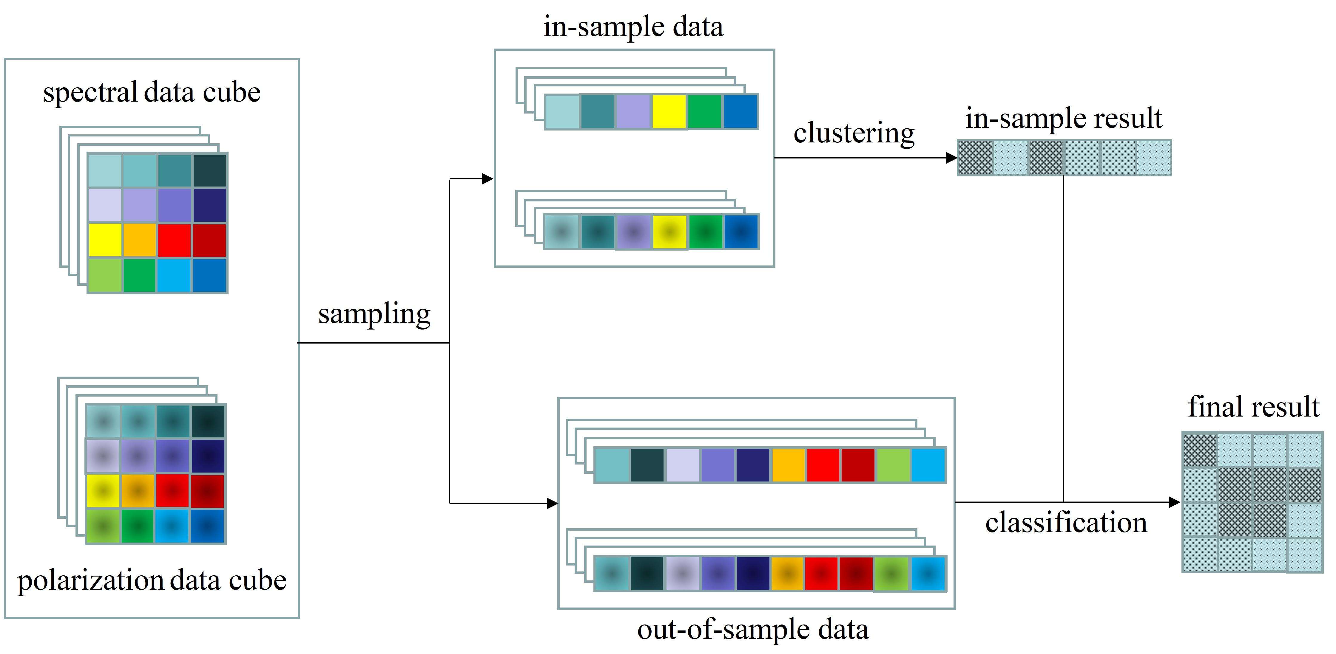
3.2. The Sampling-Clustering-Classification Strategy

Due to the large size of polarized hyperspectral images, representation-based subspace clustering programs usually require a large computer memory and long computing time, which is not in line with actual needs. For example, if the size of image is 512 * 512, the coefficient matrix C will be a 262,144 * 262,144 matrix which makes clustering a hard task. In some related works, superpixel theory is used to reduce the time complexity and space complexity of algorithms [22,23]. However, even if we reduce the size of the input data from 512 * 512 pixels to thousands of superpixels, it will still take a lot of time to solve the optimization problem. For this reason, taking the SSC model as an example, a new sampling-clustering-classifying strategy is proposed and the PS-SSC based on this strategy is called Fast Polarized Spectral Sparse Subspace Clustering (FPS-SSC).

The first step of FPS-SSC algorithm is sampling. The original polarized hyperspectral images are firstly segmented by simple linear iterative clustering (SLIC) algorithm into $N_1$ superpixels S = [S₁, S₂, … $S_{N_1}$] [24]. Then, we select a small number of data points as in-sample data and apply the PS-SSC algorithm over them. It is a challenging problem to select some key points as in-sample data. Although random sampling performs well in some cases, there is still some instability [25]. Due to the spatial characteristics of HSIs, here we propose a superpixel-based method to select in-sample data and its architecture is as shown in Figure 2.

In addition to the superpixel segmentation mentioned above, the SLIC is applied a second time to segment the original images into another superpixel set S′=[S′₁, S′₂, ⋯ S′_N2] with a number of $N_2$ which is much fewer than $N_1$. We can easily get the geometric center coordinates $GC{}^{\prime }=\left[\right(x{}^{\prime }{}_1{,y{}^{\prime }}_1){,(x{}^{\prime }}_2{,y{}^{\prime }}_2),\cdots {,(x{}^{\prime }}_{N_2}{,y{}^{\prime }}_{N_2})]$ of each superpixel of $S{}^{\prime }$. Then, the geometric centers $GC{}^{\prime }$ are projected to the superpixel set $S$, and the superpixels in which the projected points located are the selected in-sample superpixels.

By applying superpixel segmentation twice, the in-sample data can be selected stably. Then we can get the cluster assignment of in-sample data by applying the PS-SSC over them, which is the second step of FPS-SSC.

Naturally, the last part of FPS-SSC is to obtain the cluster membership of out-of-sample data by performing classification over it. Inspired by [25], we apply collaborative representation-based classification to measure the adjacency relationship among data points. In addition, the collaborative representation-based classification algorithm is modified to accommodate polarized hyperspectral images.

For each out-of-sample data we can get the representation matrix $c_i$ regarding all in-sample data as a dictionary:

$${\min }_{c_i}{\Vert c_i\Vert }_2^2+{\beta }_1{\Vert O_i^{(s)}-I^{(s)}{c}_i\Vert }_2^2+{\beta }_2{\Vert O_i^{(p)}-I^{(p)}{c}_i\Vert }_2^2,$$

(10)

where $O_i^{\left(s\right)}$ and $O_i^{\left(p\right)}$ are the spectral data and the polarization data of each out-of-sample data $O_i$, $I^{\left(s\right)}$ and $I^{\left(p\right)}$ are the spectral data and the polarization data of all in-sample data, respectively.

The solution of optimization problem (10) can be written as:

$$c_i^{\ast }={[{\beta }_1{(I^{(s)})}^T{I}^{(s)}+{\beta }_2{(I^{(p)})}^T{I}^{(p)}+I]}^{-1}[{\beta }_1{(I^{(s)})}^T{O}_i^{(s)}+{\beta }_2{(I^{(p)})}^T{O}_i^{(p)}].$$

(11)

Once the optimal $c_i^{\ast }$ is achieved, for each cluster $R_k$, the residual between $O_i$ and the in-sample points in $R_k$ can be obtained as:

$$r_k(O_i)=\frac{{\beta }_1{\Vert O_i^{(s)}-I^{(s)}{D}_k(i,j)c_i^{\ast }\Vert }_2+{\beta }_2{\Vert O_i^{(p)}-I^{(p)}{D}_k(i,j)c_i^{\ast }\Vert }_2}{{\Vert D_k(i,j)c_i^{\ast }\Vert }_2},$$

(12)

where $D_k$ is a diagonal matrix based on the in-sample clustering result:

$$D_k(i,j)=\{\begin{array}{l}1,\hspace{0.17em}\hspace{0.17em}\hspace{0.17em}i=j,\hspace{0.17em}\mathrm{and}\hspace{0.17em}j\mathrm{th}\hspace{0.17em}\mathrm{in}-\mathrm{sample}\hspace{0.17em}\mathrm{data}\hspace{0.17em}\mathrm{belongs}\hspace{0.17em}\mathrm{to}\hspace{0.17em}k\mathrm{th}\hspace{0.17em}\mathrm{cluster}\\ 0,\hspace{0.17em}\hspace{0.17em}\hspace{0.17em}\mathrm{otherwise}\end{array}.$$

(13)

$O_i$ is then matched into the cluster that has the minimum residual:

$$identity(O_i)=\underset{k}{\arg \min }[r_k(O_i)],$$

(14)

where identity(O_i) denotes the assignment of the out-of-sample data O_i, which means O_i belongs to kth cluster if $r_k\left(O_i\right)$ is the minimum value of ${\left\{r_k\left(O_i\right)\right\}}_{k=1}^K$.

The proposed efficient clustering framework for polarized hyperspectral images is also scalable to LRR, LSR and other representation-based subspace clustering models. In addition, algorithms applying this framework can be summarized as Algorithm 1.

Algorithm 1 FPS-SSC, FPS-LRR and FPS-LSR

Input:     Spectral dataset $Y^{\left(s\right)}$ and polarized dataset $Y^{\left(p\right)}$; the desired number of clusters $k$, ${\lambda }_1$, ${\lambda }_2$, ${\sigma }_s$, ${\sigma }_p$, ${\beta }_1$ and ${\beta }_2$. Main algorithm: (1) Sampling: apply the superpixel-based method to segment images into $N_1$ superpixels and to select $N_2$ in-sample data. (2) Clustering: perform polarized hyperspectral clustering algorithm (PS-SSC or PS-LRR or PS-LSR) over in-sample data. (3) Classification: match each out-of-sample data into the clusters of in-sample data with (10)–(14). Output:     A 2-D matrix which records the labels of the clustering result of the polarized hyperspectral images.

4. Experimental Results and Discussion

In this section, some experiments are carried out to demonstrate the accuracy, efficiency and potential capabilities of the proposed polarized hyperspectral clustering framework. As described above, this method can be applied to most representation-based clustering algorithms. Here we mainly use the polarized spectral version and fast polarized spectral version of SSC as examples, and take LRR and LSR as supplementary analysis. We also compare the clustering performance of these methods with a benchmark method k-means and a novel non-subspace based clustering algorithm rank-two nonnegative matrix factorization (R2NMF) [26].

This section consists of four parts. Section 1 introduces the datasets we used for experiments, and Section 2 shows the clustering results of different algorithms. The analyses of sensitivity of parameters and selection of in-sample data and the number of superpixels are in Section 3 and Section 4, respectively.

4.1. Instrument and Data

In order to evaluate the performance of the proposed method, here we obtained two polarized hyperspectral datasets. Dataset A was measured with a channeled interference imaging spectropolarimeter (CIISP) proposed by Zhang et al. The CIISP can simultaneously obtain four stokes vectors (${\mathrm{S}}_0$, ${\mathrm{S}}_1$, ${\mathrm{S}}_2$ and ${\mathrm{S}}_3$) in 128 wave bands from 480 to 960 nm of a two-dimensional space target through one-dimensional push sweep. The experimental data was collected by the authors of this paper at a distance of 2 km, and the size of images is 512 × 512. Since the CIISP instrument is designed for spaceborne, collected images at this distance are somewhat blurred. This point posed a challenge to the clustering accuracy of the algorithms.

Dataset B that includes four polarization angles ($0°,45°,90°,\mathrm{and}135°$) in 33 bands from 400 to 720 nm is from the Northwestern Polytechnical University, and can be downloaded from the website (http://jszy.nwpu.edu.cn/zhaoyq.html).

After getting four stokes vectors, since ${\mathrm{S}}_3$ is usually negligible under natural conditions, the degree of linear polarization ($\mathrm{DOLP}$) can be obtained by:

$$\mathrm{DOLP}=\frac{\sqrt{{\mathrm{S}}_1^2+{\mathrm{S}}_2^2}}{{\mathrm{S}}_0}.$$

(15)

Then we can regard ${\mathrm{S}}_0$ as ordinary hyperspectral information and the $\mathrm{DOLP}$ as polarization information. Figure 3a–d shows the ${\mathrm{S}}_0$ and $\mathrm{DOLP}$ images of dataset A at 690 and 778 nm, and Figure 3e–h shows the ${\mathrm{S}}_0$ and $\mathrm{DOLP}$ images of dataset B at 480 and 690 nm.

Based on the SLIC algorithm, three bands (RGB) of ${\mathrm{S}}_0$ were selected to construct a false color image, and then the false color image was segmented into thousands of superpixels. Note that for dataset A, since the spectral range (480–960 nm) of the CIISP does not include 435.8 nm which means red, the false color image is just an approximation. In the case where the number of superpixels is too small, there will be a sacrifice of image spatial resolution, which leads to a reduction in clustering accuracy. While if the number is too large, the computational time required for clustering will increase dramatically. In this paper, the number was placed at about 3000. Figure 3j,l shows the superpixel segmentation results.

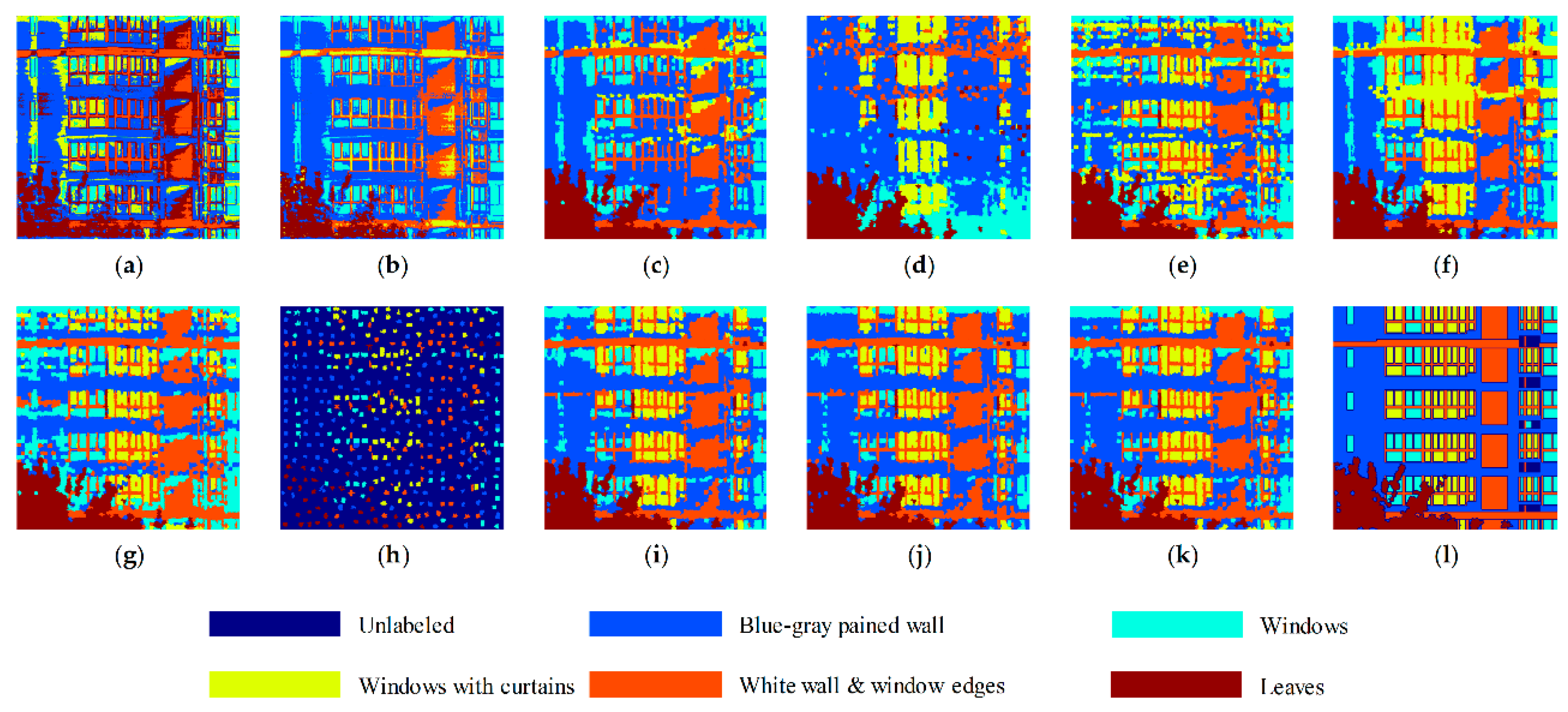
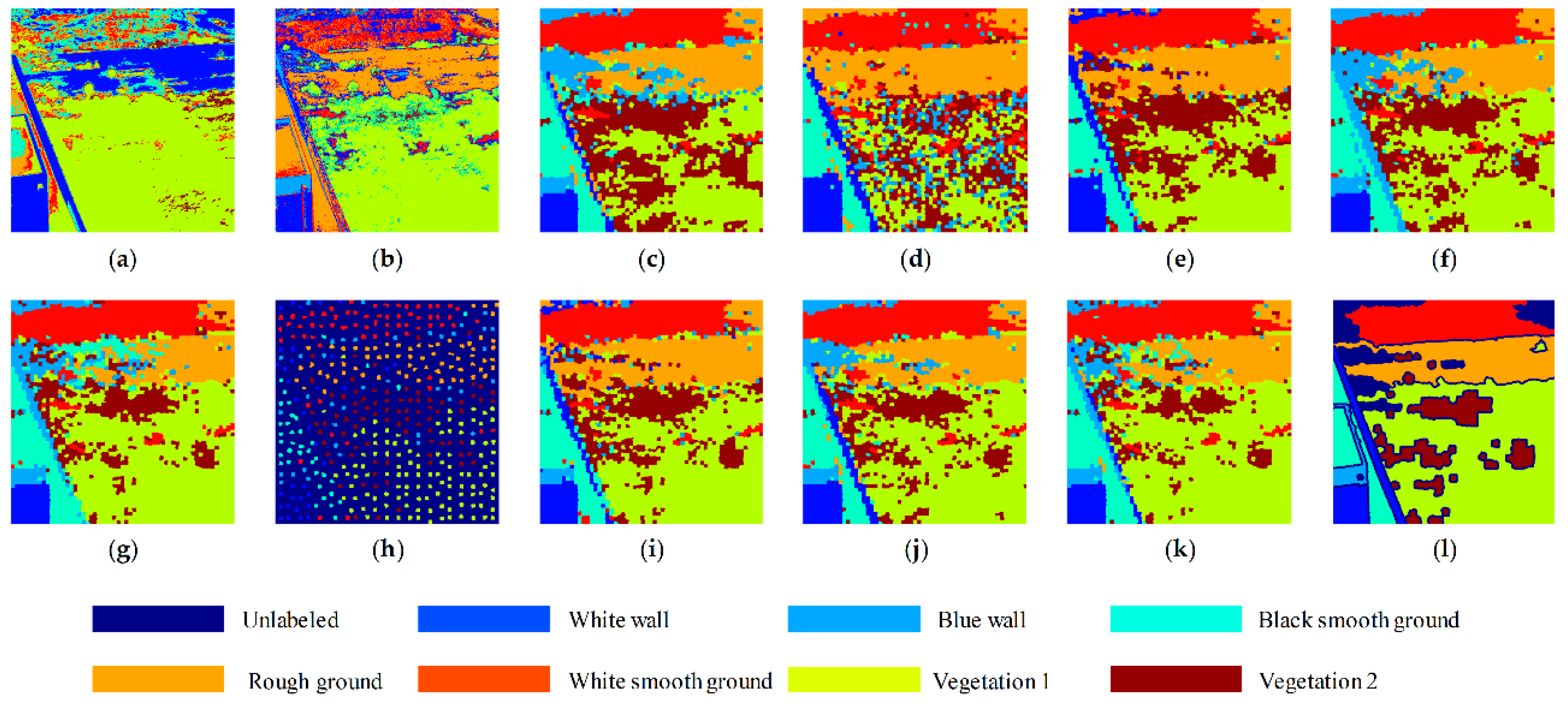
4.2. Clustering Results and Discussion

Dataset A includes five different kinds of targets: blue-gray painted wall; windows without curtains; windows with curtains; white painted wall and window edges; and leaves. Although the window edges are composed of metal, the surface is a layer of white paint, so it belongs to the same cluster as the white painted wall. Additonally, if there are curtains in the window, a large part of the light passing through the glass window will be reflected by the curtains, otherwise the light will enter the room and only a small part will be reflected back. Therefore, the existence of curtains will cause the difference in ${\mathrm{S}}_0$ and $\mathrm{DOLP}$ intensity. In addition, dataset B includes seven kinds of targets: white wall, blue wall, white smooth ground, black smooth ground, rough ground, vegetation 1 and vegetation 2.

The cluster maps of the various clustering methods of dataset A and dataset B are shown in Figure 4 and Figure 5, respectively, and the corresponding quantitative evaluation of the clustering results is provided in

Table 2. Quantitative evaluation of the different clustering algorithms of dataset A.

Method	Classes	k-Means	R2NMF	SSC-S0	SSC-DOLP	PS-SSC	PS-LRR	PS-LSR	FPS-SSC	FPS-LRR	FPS-LSR
AC (%)	Blue-gray painted wall	69.93	81.67	73.24	10.05	63.18	62.94	57.14	80.70	84.31	79.63
	Windows	50.94	76.90	79.74	64.75	72.99	81.28	84.29	70.18	59.60	64.40
	Windows with curtains	30.72	0.07	1.78	89.08	69.40	88.99	73.37	83.59	81.65	81.86
	White wall and window edges	45.94	52.18	65.71	13.50	64.60	66.12	76.52	71.93	75.85	76.77
	Leaves	73.60	77.07	98.58	97.46	97.69	96.12	95.44	96.34	94.87	96.04
OA (%)		57.49	63.25	66.02	35.84	69.07	72.46	71.02	79.44	80.40	79.36
Running time (s)		31.32	18.03	230.2	223.2	378.6	371.3	112.9	58.33	59.89	55.00

and

Table 3. Quantitative evaluation of the different clustering algorithms of dataset B.

Method	Classes	k-means	R2NMF	SSC-S0	SSC-DOLP	PS-SSC	PS-LRR	PS-LSR	FPS-SSC	FPS-LRR	FPS-LSR
AC(%)	White wall	95.95	71.75	80.88	88.77	89.45	58.04	58.04	86.16	90.90	64.37
	Blue wall	0	74.02	71.69	0.00	0.00	81.89	75.09	63.59	69.19	74.87
	Black smooth ground	14.57	0	93.29	91.26	87.92	91.43	92.46	91.30	91.39	93.26
	White smooth ground	90.56	84.58	90.89	87.01	89.49	91.73	91.15	89.20	91.96	91.80
	Rough ground	2.54	81.62	81.57	95.82	93.87	81.52	62.99	93.71	86.20	76.55
	Vegetation 1	18.42	46.10	62.09	42.03	71.70	75.53	88.21	80.82	82.79	90.56
	Vegetation 2	0.51	10.90	89.57	51.05	89.48	85.61	72.42	82.22	79.12	65.31
OA (%)		50.11	64.61	75.70	64.04	80.68	80.20	81.46	85.10	85.28	84.58
Running time (s)		11.05	8.35	235.2	219.2	369.6	373.2	115.6	55.45	59.81	44.03

. Considering the limitations of the spatial resolution of the instruments themselves, it is difficult to evaluate the clustering performance at the boundary of the two targets and some vague areas, so these pixels which are unlabeled in Figure 4j and Figure 5j were ignored when calculating the accuracy (AC).

It can be obviously observed from Table 2 and Table 3 that adding polarization into HSIs’ clustering improved the overall accuracy (OA) significantly. For dataset A, directly applying the SSC algorithm over the ${\mathrm{S}}_0$ dataset can distinguish between blue-gray painted wall, windows without curtains, white painted wall and window edges, leaves, but the accuracy of windows with curtains is only 1.78%. While directly applying the SSC algorithm over the $\mathrm{DOLP}$ dataset can achieve a high accuracy of 89.08% on windows with curtains with low accuracy on blue-gray painted wall, windows without curtains, white painted wall and window edges. Both of two methods perform well on leaves, because leaves have distinct features on ${\mathrm{S}}_0$ and $\mathrm{DOLP}$. As a combination of spectral information and polarized information, the PS-SSC algorithm has the advantages of SSC (${\mathrm{S}}_0$) and advantages of SSC ($\mathrm{DOLP}$) simultaneously. The accuracy of windows with curtains is 86.15% and the accuracy of other classes remains at a good level, which leads to a higher OA. It is similar for PS-LRR and PS-LSR that reach 72.46% and 71.02% of OA, respectively.

The dataset B does not have the window with curtains which is totally different from other targets in $\mathrm{DOLP}$ as in dataset A. Except for the edge contour, the $\mathrm{DOLP}$ intensity of different targets in dataset B is not significantly different. In this case, as can be seen from Table 3, adding polarization still improves the accuracy of clustering by about 5%.

However, on the other hand, due to the complexity of the optimization process, the time cost of these three methods is too high. The PS-SSC and the PS-LRR take more than 350 s of running time, and even though there is no iteration in solving the optimization problem in the PS-LSR algorithm, it still takes about 2 min. The k-means takes much less time than these subspace-based methods, but the OAs in both two datasets are much lower. Although the R2NMF can reach a higher OA than k-means with less running time, its OA is still not as good as subspace-based methods.

When the sampling-clustering-classification strategy is adopted, the running time is greatly reduced to less than 1 min. The FPS-SSC, FPS-LRR and FPS-LSR all achieved OAs of about 80% on dataset A and 85% on dataset B, which are even much higher than the PS-SSC, PS-LRR and PS-LSR. The PS version algorithms are equivalent to taking all 3249 superpixels as in-sample data in FPS version algorithms. Usually, for sampling strategies, the more sampling points there are, the higher the accuracy should be. However, the experimental results show a different trend. This is because the representation-based models themselves can achieve high accuracies on small-scale datasets, but on large-scale datasets, they may not perform as well as on small-scale ones. In addition to reducing the computational complexity, this is another reason why we adopt a sampling strategy to avoid clustering directly on polarized hyperspectral datasets. The relationship between OA and the number of selected in-sample data is discussed in Section 4.

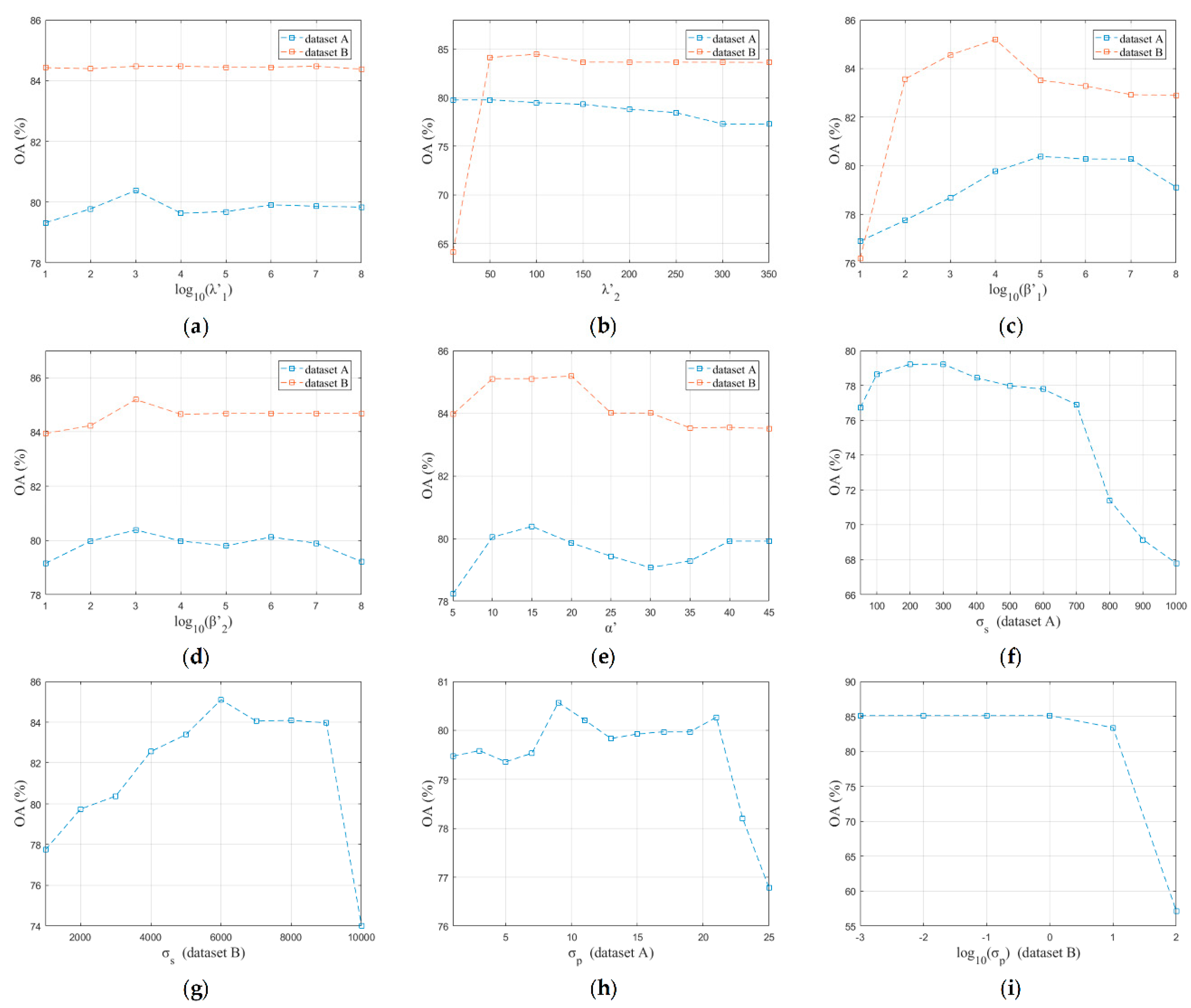
4.3. Sensitivity of Parameters

Obviously, the various parameters required in the algorithms have an important impact on the final clustering results. In different practical application scenarios, the parameters need to be reset. It is desired for parameters to achieve the best performance by taking the same values on different datasets, so that users can easily set the parameters when applying these algorithms on various datasets collected by different instruments and different measurement environments.

In addition to the number of in-sample data, there are five trade-off parameters ($\alpha$, ${\lambda }_1$, ${\lambda }_2$, ${\beta }_1$ and ${\beta }_2$) and two weight parameters (${\sigma }_s$ and ${\sigma }_p$) in the proposed framework. For subspace clustering algorithms, regularization parameter $\lambda$ is decided by the following formulation [13]:

$$\lambda =\frac{{\lambda }^{\prime }}{\mu },$$

(16.a)

$$\mu =\underset{i}{\min } \underset{j\ne i}{\max }\left|y_i^T{y}_j\right|,$$

(16.b)

where $\lambda {}^{\prime }$ is the adjustment coefficient and $\mu$ is fixed for a certain dataset. The five trade-off parameters, extending (16.a) and (16.b) to them, can be replaced with parameters not related to the dataset by:

$${\lambda }_1=\frac{{{\lambda }^{\prime }}_1}{\underset{i}{\min } \underset{j\ne i}{\max }\left|Y_i^{(s)}{}^T{Y}_j^{(s)}\right|},$$

(17.a)

$${\lambda }_2=\frac{{{\lambda }^{\prime }}_2}{\underset{i}{\min } \underset{j\ne i}{\max }\left|Y_i^{(p)}{}^T{Y}_j^{(p)}\right|},$$

(17.b)

$${\beta }_1=\frac{{{\beta }^{\prime }}_1}{\underset{n}{\min } \underset{m\ne n}{\max }\left|O_{i_m}^{(s)}{}^T{I}_n^{(s)}\right|},$$

(17.c)

$${\beta }_2=\frac{{{\beta }^{\prime }}_2}{\underset{n}{\min } \underset{m\ne n}{\max }\left|O_{i_m}^{(p)}{}^T{I}_n^{(p)}\right|},$$

(17.d)

$$\alpha ={\alpha }^{\prime }\frac{\underset{i}{\min } \underset{j\ne i}{\max }\left|{(W_p{C}^{(s)})}_i^T{(W_p{C}^{(s)})}_j\right|}{\underset{i}{\min } \underset{j\ne i}{\max }\left|{(W_s{C}^{(p)})}_i^T{(W_s{C}^{(p)})}_j\right|}.$$

(17.e)

By changing one of those parameters while other parameters are fixed, the sensitivity of this parameter is determined. A change curve of the overall accuracy and in-sample accuracy with various values of different parameters is drawn in Figure 6.

Taking the OA of 79% or more of dataset A and the OA of 83% or more of dataset B as acceptable ranges, we can get the following phenomena from Figure 6:

(1) ${\lambda }_1{}^{\prime }$ performs well on dataset A and dataset B in the range of eight orders of magnitude (10–10⁸) with the peaks at 10³, and ${\lambda }_2{}^{\prime }$ can keep a high level of OA for both datasets in the range of 50–200;

(2) ${\beta }_1{}^{\prime }$ can reach the acceptable OA taking value from 10² to 10⁶ for dataset A and from 10⁴ to 10⁸ for dataset B, and ${\beta }_2{}^{\prime }$ meets this requirement in eight orders of magnitude (10–10⁸) with the peaks at 10³ for both datasets;

(3) $\alpha {}^{\prime }$ can achieve the highest OA for the two datasets in the range of 10–20, and the peaks appear when $\alpha {}^{\prime }$ is 15;

(4) For ${\sigma }_s$ and ${\sigma }_p$, it is difficult to find fixed values for different datasets like the trade-off parameters, but they have a wide range of acceptable values on each dataset.

Summarizing the above points, we can reach the conclusion that the five trade-off parameters (${\lambda }_1{}^{\prime }$, ${\lambda }_2{}^{\prime }$, ${\beta }_1{}^{\prime }$, ${\beta }_2{}^{\prime }$ and $\alpha {}^{\prime }$) and the two weight parameters (${\sigma }_s$ and ${\sigma }_p$) all have low parameter sensitivity. In addition, especially for the trade-off parameters, the best values on different datasets are very close.

4.4. Selection of In-Sample Data and the Number of Superpixels

In the proposed framework, images are firstly segmented into lots of superpixels by the SLIC algorithm. Intuitively, the final OA as well as the running time is closely related to the number of superpixels. Figure 7a,b respectively indicates the OA and running time of FPS-SSC, FPS-LRR, FPS-LSR in the cases where the numbers of superpixels are 1024, 3249, 5329, 7225 and 10,404 when the number of in-sample points is 429. As the number of superpixels increases, the OA does not keep increasing but remains at a stable level when the number is greater than 3000. While, the running time grows up monotonically with the number of superpixels. Therefore, as a trade-off choice, the suggested number of superpixels for 512 × 512 images is 2000–5000.

The OA also depends on the selection method of the in-sample data. Figure 7c shows the comparison between random sampling and the superpixel-based method presented in Section 3, and the red dotted line indicates the mean and standard deviation of the results of applying FPS-SSC algorithm with random sampling for 10 times. Since the random sampling method is not in a position to ensure if the selection of in-sample data is suitable, it is accompanied by large standard deviation and great uncertainty. While applying the superpixel-based method, although its OA may be lower than the best results of random sampling, it achieves more than 75% of OA under different numbers of sampling data, and the results are much higher than the mean of the results of random sampling. Another benefit of the superpixel-based method is the stability, which means we only need one experiment to get a reliable clustering result.

In addition, the clustering result relies on the number of in-sample data. The number of in-sample data affects the OA in two ways: (1) as the number increases, the OA generally shows an upward trend; (2) the number also affects the clustering accuracy of in-sample data, which is another important factor in OA. Figure 7d indicates the OA of FPS-SSC, FPS-LRR, FPS-LSR in the cases where the numbers of in-sample data are 214, 309, 429, 509, 622 and 764. Additionally, Figure 7e,f shows the corresponding In-sample Accuracy (IA) and running time, respectively. From the trend point of view, when the value of A is larger, the larger the OA. However, when the number takes values 509 and 622, the OA drops. This happens because when the number equals to 509 or 622, the accuracy of in-sample data is significantly reduced.

Additionally, as expected, the running time increases monotonically with the number of in-sample data. Following consideration of the cost of time, the suggested number of in-sample data is about one tenth of the number of superpixels. Specifically, for images with a size of 512 × 512, a high OA as well as relatively short running time can be achieved when the number of in-sample data is 400–500.

5. Conclusions

In this paper, we added polarization into the clustering of hyperspectral images and proposed a representation-based subspace clustering framework for polarized hyperspectral images by treating each kind of land-cover class as a subspace. Furthermore, faced with the shortcoming that representation-based subspace clustering requires too much running time, an improved efficient version adopting the sampling-clustering-classification strategy was presented. Extensive experimental results clearly show that algorithms using proposed framework (FPS-SSC, FPS-LRR, FPR-LSR) can achieve a superior clustering performance with short running time and low sensitivity of parameters.

The proposed method can be further improved by the adaptive determination of the weight parameters and automatic determination of the cluster number by subspace detection, which will be in our future work.

References

1. Curran, P.J. A photographic method for the recording of polarized visible light for soil surface moisture indications. Remote Sens. Environ. 1978, 7, 305–322. [Google Scholar] [CrossRef]
2. Deschamps, P.-Y. The POLDER mission: Instrument characteristics and scientific objectives. IEEE Trans. Geosci. Remote Sens. 1994, 32, 598–615. [Google Scholar] [CrossRef]
3. Wolff, L.B. Polarization-based material classification from specular reflection. IEEE Trans. Pattern Anal. Mach. Intell. 1990, 12, 1059–1071. [Google Scholar] [CrossRef]
4. Wolff, L.B.; Boult, T.E. Constraining object features using a polarization reflectance model. IEEE Trans. Pattern Anal. Mach. Intell. 1991, 13, 635–657. [Google Scholar]
5. Palubinskas, G.; Datcu, M.; Pac, R. Clustering algorithms for large sets of heterogeneous remote sensing data. Proc. IGARSS 1999, 3, 1591–1593. [Google Scholar]
6. Barni, M.; Garzelli, A.; Mecocci, A.; Sabatini, L. A robust fuzzy clustering algorithm for the classification of remote sensing images. Proc. IGARSS 2000, 5, 2143–2145. [Google Scholar]
7. Paoli, A.; Melgani, F.; Pasolli, E. Clustering of Hyperspectral Images Based on Multiobjective Particle Swarm Optimization. IEEE Trans. Geosci. Remote Sens. 2009, 47, 4175–4188. [Google Scholar] [CrossRef]
8. Li, S.; Zhang, B.; Li, A.; Jia, X. Hyperspectral imagery clustering with neighborhood constraints. IEEE Geosci. Remote Sens. Lett. 2013, 10, 588–592. [Google Scholar] [CrossRef]
9. Bo, R.; Biao, H. Sparse Subspace Clustering-Based Feature Extraction for PolSAR Imagery Classification. Remote Sens. 2018, 10, 391. [Google Scholar] [Green Version]
10. Murphy, J.M.; Maggioni, M. Unsupervised Clustering and Active Learning of Hyperspectral Images with Nonlinear Diffusion. IEEE Trans. Geosci. Remote Sens. 2019, 57, 1829–1845. [Google Scholar] [CrossRef]
11. Saranathan, A.M.; Parente, M. On Clustering and Embedding Mixture Manifolds using a Low Rank Neighborhood Approach. IEEE Trans. Geosci. Remote Sens. 2019, 57, 3890–3903. [Google Scholar] [CrossRef]
12. Chunmin, Z.; Qiwei, L. High throughput static channeled interference imaging spectropolarimeter based on a Savart polariscope. Opt. Express 2016, 24, 23314–23332. [Google Scholar]
13. Elhamifar, E.; Vidar, R. Sparse subspace clustering: Algorithm, theory, and application. IEEE Trans. Pattern Anal. Mach. Intell. 2013, 35, 2765–2781. [Google Scholar] [CrossRef] [PubMed]
14. Liu, G.C.; Lin, Z.C.; Yu, Y. Robust subspace segmentation by low-rank representation. In Proceedings of the 27th International Conference on Machine Learning (ICML), Haifa, Israel, 21–24 June 2010; pp. 663–670. [Google Scholar]
15. Canyi, L.; Hai, M. Robust and efficient subspace segmentation via least squares regression. In Proceedings of the 12th European Conference on Computer Vision, Florence, Italy, 7–13 October 2012; pp. 347–360. [Google Scholar]
16. Zhang, H.; Zhai, H.; Zhang, L.; Li, P. Spectral-spatial sparse subspace clustering for hyperspectral remote sensing images. IEEE Trans. Geosci. Remote Sens. 2016, 54, 3672–3684. [Google Scholar] [CrossRef]
17. Zhai, H.; Zhang, H.; Zhang, L.; Li, P.; Plaza, A. A new sparse subspace clustering algorithm for hyperspectral remote sensing imagery. IEEE Geosci. Remote Sens. Lett. 2017, 14, 43–47. [Google Scholar] [CrossRef]
18. Afonso, M.V.; Bioucas-Dias, J.M.; Figueiredo, M.A.T. An augmented Lagrangian approach to the constrained optimization formulation of imaging inverse problems. IEEE Trans. Image Process. 2011, 20, 681–695. [Google Scholar] [CrossRef] [PubMed]
19. Mota, J.F.; Xavier, J.W.F.; Aguiar, P.M.Q.; Puschel, M. D-ADMM: A communication-efficient distributed algorithm for separable optimization. IEEE Trans. Signal Process. 2013, 61, 2718–2723. [Google Scholar] [CrossRef]
20. Shi, J.; Malik, J. Normalized cuts and image segmentation. IEEE Trans. Pattern Anal. Mach. Intell. 2000, 22, 888–905. [Google Scholar]
21. Ng, A.Y.; Jordan, M.I.; Weiss, Y. On spectral clustering: Analysis and an algorithm. Proc. Adv. Neural Inf. Process. Syst. 2002, 2, 849–856. [Google Scholar]
22. Zhang, G.; Jia, X.; Kwok, N.M. Super pixel based remote sensing image classification with histogram descriptors on spectral and spatial data. In Proceedings of the IEEE International Geoscience and Remote Sensing Symposium, Munich, Germany, 22–27 July 2012; pp. 4335–4338. [Google Scholar]
23. Zhang, G.; Jia, X.; Hu, J. Superpixel-based graphical model for remote sensing image mapping. IEEE Trans. Geosci. Remote Sens. 2015, 53, 5861–5871. [Google Scholar] [CrossRef]
24. Radhakrishna, A. SLIC Superpixels Compared to State-of-the-art Superpixel Methods. IEEE Trans. Pattern Anal. Mach. Intell. 2012, 34, 2274–2282. [Google Scholar]
25. Peng, X.; Zhang, L.; Yi, Z. Scalable sparse subspace clustering. In Proceedings of the 26th IEEE Conference on Computer Vision and Pattern Recognition, Portland, OR, USA, 23–28 June 2013; pp. 430–437. [Google Scholar]
26. Gillis, N.; Kuang, D.; Park, H. Hierarchical Clustering of Hyperspectral Images Using Rank-Two Nonnegative Matrix Factorization. IEEE Trans. Geosci. Remote Sens. 2015, 53, 2066–2078. [Google Scholar] [CrossRef]
Figure 1. Architecture of proposed efficient representation-based subspace clustering framework for polarized hyperspectral images.
Remotesensing 11 01513 g001
Figure 2. Architecture of proposed superpixel-based selection method of in-sample data.
Remotesensing 11 01513 g002
Figure 3. Images of dataset A and dataset B: (a) S 0 image of dataset A at 690 nm; (b) degree of linear polarization ( DOLP ) image of dataset A at 690 nm; (c) S 0 image of dataset A at 778 nm; (d) DOLP image of dataset A at 778 nm; (e) S 0 image of dataset B at 480 nm; (f) DOLP image of dataset B at 480 nm; (g) S 0 image of dataset B at 690 nm; (h) DOLP image of dataset B at 690 nm; (i) false color image of dataset A; (j) 3249 superpixels of dataset A; (k) false color image of dataset B; (l) 3249 superpixels of dataset B.
Remotesensing 11 01513 g003
Figure 4. Cluster maps of the different methods of dataset A: (a) k-means with S 0 dataset only; (b) rank-two nonnegative matrix factorization (R2NMF) with S 0 dataset only; (c) sparse subspace clustering (SSC) with S 0 dataset only; (d) SSC with DOLP dataset only; (e) Polarized Spectral -SSC; (f) PS-low-rank representation subspace segmentation (LRR); (g) PS-least squares regression subspace segmentation (LSR); (h) in-sample clustering result of Fast Polarized Spectral (FPS)-SSC; (i) FPS-SSC; (j) FPS-LRR; (k) FPS-LSR; (l) ground truth.
Remotesensing 11 01513 g004
Figure 5. Cluster maps of the different methods of dataset B: (a) k-means with S 0 dataset only; (b) R2NMF with S 0 dataset only; (c) SSC with S 0 dataset only; (d) SSC with DOLP dataset only; (e) PS-SSC; (f) PS-LRR; (g) PS-LSR; (h) in-sample clustering result of FPS-SSC; (i) FPS-SSC; (j) FPS-LRR; (k) FPS-LSR; (l) ground truth.
Remotesensing 11 01513 g005
Figure 6. Analysis of parameters. Change in the overall accuracy and in-sample accuracy with various values of: (a) λ 1 of dataset A and dataset B; (b) λ 2 of dataset A and dataset B; (c) β 1 of dataset A and dataset B; (d) β 2 of dataset A and dataset B; (e) α of dataset A and dataset B; (f) σs of dataset A; (g) σs of dataset B; (h) σp of dataset A; (i) σp of dataset B.
Remotesensing 11 01513 g006
Figure 7. Analysis of the number of superpixels and the selection of in-sample data: (a) change in overall accuracy (OA) with various numbers of superpixels; (b) change in running time with various numbers of superpixels; (c) comparison between random sampling and proposed method; (d) change in OA with various numbers of in-sample data; (e) change in In-sample Accuracy (IA) with various numbers of in-sample data; (f) change in running time with various numbers of in-sample data.
Remotesensing 11 01513 g007