A Simple Similarity Index for the Comparison of Remotely Sensed Time Series with Scarce Simultaneous Acquisitions

Abstract

Emergence of new state-of-the-art technologies has enabled an unprecedented amount of high spatial resolution satellite data having great potential for exploitation of extracted time series for a vast range of applications. Despite the high temporal resolution of time series, the number of real observations of optical data that can be utilized is reduced due to meteorological conditions (such as cloud or haze) prevailing at the time of acquisition. This fact has an effect on the density of the retrieved time series and subsequently on a number of coincidental observations when comparing the similarity of time series from two different data sources for which the simultaneous acquisition date is already scarce. Classical tools for assessing the similarity of such time series can prove to be difficult or even impossible because of a lack of simultaneous observations. In this paper, we propose a simple method in order to circumvent this scarcity issue. In the first step, we rely on an interpolation in order to produce artificial time series on the union of the original acquisition dates. Then, we extend the theory of the correlation coefficient (CC) estimator to these interpolated time series. After validation on synthetic data, this simple approach proved to be extremely efficient on a real case study where Sentinel-2 and PlanetScope NDVI time series on parcels in The Netherlands are compared. Indeed, compared to other methods, it reduced the number of undecided cases while also improving the power of the statistical test on the similarity between both types of time series and the precision of the estimated CC.

1. Introduction

Time series consist of repeated observations of the same quantity of interest over time. Often, these quantities are sampled on a regular time step (e.g., every minute/hour/day/week/month/year) so that one can define the notion of “next observation” or “previous observation” within the time series. While classical time series analysis and time series model generally assume these particular and optimal conditions [1]; such conditions are not always encountered in real-world applications, e.g., in remote sensing. Remote sensing time series are generally built with images acquired at very specific dates that depend on the revisit time of the sensor. There is often a trade-off between spatial resolution and revisit time so the issue is particularly seen for high (HR) and very high resolution (VHR) images [2,3]. In addition, it is also quite common for some of the observations to be discarded because of the poor data quality (e.g., cloud cover, haze). Finally, as Earth Observation (EO) scientists generally rely on different sensors, multivariate time series analyses can rapidly become complicated because not only are the acquisition dates not equidistant within each time series, but it is also unlikely to have a match between the different sets of acquisition dates. In particular, this has important practical impacts when we want to measure the similarity between time series.

The classical tool for quantifying the similarity between time series is to estimate the temporal structure of the time series through their empirical autocorrelation function and their empirical cross-correlation function [4]. In both cases, the idea is to estimate the correlation coefficients (CC) between observations distant of a given time lag. For irregularly sampled time series, one can rely on slotting methods that consist of grouping pairs of observations in classes of time distance [5]. The same approach is used for the estimation of covariograms and semivariograms for spatial data [4]. Unfortunately, these approaches generally require at least 30 pairs of observations in each of the classes in order to obtain reliable estimations [6]. This is a major limitation for their application in the context of scarcely sampled time series. Alternatively, one would like to limit the similarity analysis on the estimated zero-lag CC (i.e., the classical CC). In any case, this is still sometimes beyond reach because of the lack of simultaneous observations. Another alternative that is inspired from speech recognition [7] is dynamic time warping (DTW). It consists in warping the time axis for an optimal alignment of the time series. It is possible to constrain the warping to consider only pairs of observations that are not too far from each other, e.g., the Sakoe–Chiba band [8]. The resulting time series share the same length but consist of padded sequences of the same values (when the time series are stretched) so the actual number of genuine observations is smaller. Recently, it has been applied to remote sensing applications as well, mainly in image classification (e.g., [8] or [9]). DTW does not directly provide an index of similarity. For that purpose, one can compute the CC between the aligned time series.

In this paper, we proposed to overcome the scarcity of the time series with a simple linear interpolation approach. The motivation is to obtain two time series with identical acquisition dates, so that the classical estimation of the CC is possible. We rely here on the CC because we are interested in the similarity between the time series (i.e., exhibiting the same patterns) compared to the more specific objectives of other existing indexes such as the index of agreement [10,11,12] where the values between the time series must be comparable in absolute terms (e.g., same average, same standard deviation,…). While the resulting time series are a mix of genuine observations and synthetic values, we think that an interpolation between two consecutive dates is a valid and natural approach at least for continuous processes (e.g., vegetation/crop monitoring). Indeed, it directly translates the cognitive mechanisms that the analyst uses when one visually compares the two time series on the same graph. We opted for linear interpolations in order to keep the method as simple as possible. However, experimental results showed that using a shape-preserving piecewise cubic interpolation did not bring significant changes (results not shown here). Alternatively, choosing more advanced interpolation methods (e.g., splines) might also be an option but there is a risk of adding artifacts in the interpolated time series [13].

After a short reminder of the theoretical characteristics of the CC estimator, the proposed approach is first tested on simulated time series with limited simultaneous observations. The results confirmed that our method provides accurate estimations of the CCs while overcoming the scarcity of the time series. The method is further illustrated on the comparison of real NDVI time series from Sentinel-2 and PlanetScope in The Netherlands, with the same results as found in the synthetic examples. Indeed, the two sets of time series were found to be very correlated, as expected (the average estimated CC was found to be equal to 0.93), while drastically reducing the number of undecided cases due to the lack of simultaneous observations (from 385 to 14 out of 1670).

2. Methodology

2.1. The Correlation Coefficient

The correlation coefficient (or Pearson’s correlation coefficient) can be used for assessing the similarity between the two time series [10]. For paired observations (i.e., each observation is a pair of both quantities), the CC is generally estimated using the following estimator

$$\widehat{\rho }=\frac{{{\displaystyle \sum }}_{i=1}^n\left(x_i-\overline{x}\right)\left(y_i-\overline{y}\right)}{\sqrt{{{\displaystyle \sum }}_{i=1}^n{\left(x_i-\overline{x}\right)}^2}\sqrt{{{\displaystyle \sum }}_{i=1}^n{\left(y_i-\overline{y}\right)}^2}},$$

(1)

where ($x_i,y_i)$ are the paired observations, $\overline{x}$ and $\overline{y}$ are the observed averages of the time series and $n$ is the number of observed pairs.

The precision of this estimator is generally evaluated using Fisher’s transformation [14]

$$\widehat{\lambda }=0.5\ln \left(\frac{1+\widehat{\rho }}{1-\widehat{\rho }}\right),$$

(2)

and its inverse transformation

$$\widehat{\rho }=\frac{e^{2\widehat{\lambda }}-1}{e^{2\widehat{\lambda }}+1}.$$

(3)

The main advantage of this transformation is that $\widehat{\lambda }$ is approximately following a normal distribution with a mean equal to $\lambda =0.5\ln \left(\frac{1+\rho }{1-\rho }\right)$ (where $\rho$ the true unknown CC) and a variance approximately equal to

$${\sigma }_{\lambda }^2={\left(n-3\right)}^{-1}.$$

(4)

One can thus build the ($1-\alpha )$ confidence interval for λ with $\widehat{\lambda }\pm \frac{z_{1-\alpha /2}}{\sqrt{n-3}}$ and use the inverse transformation in order to get the confidence interval for $\rho$

$$C{I}_{\rho }=\left[\frac{e^{2{\widehat{\lambda }}_L}-1}{e^{2{\widehat{\lambda }}_L}+1};\frac{e^{2{\widehat{\lambda }}_U}-1}{e^{2{\widehat{\lambda }}_U}+1}\right],$$

(5)

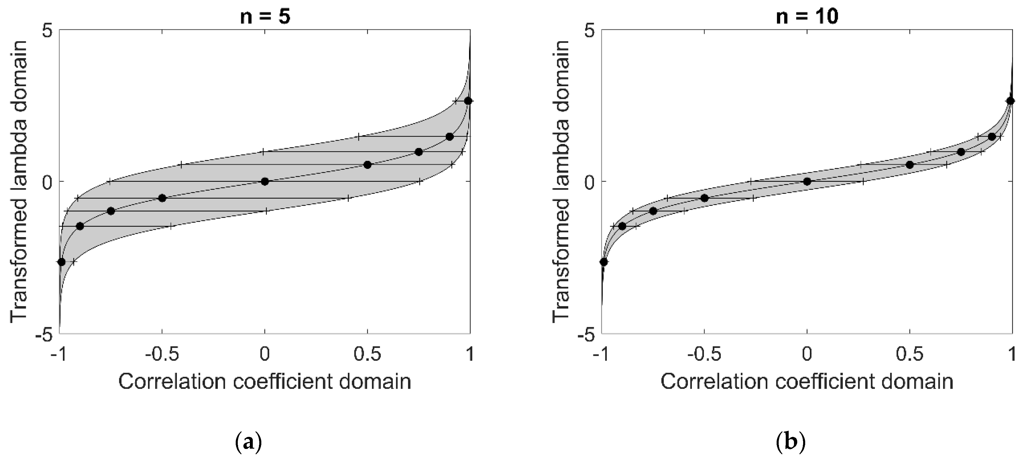
where ${\widehat{\lambda }}_L=\widehat{\lambda }-\frac{z_{1-\alpha /2}}{\sqrt{n-3}}$, ${\widehat{\lambda }}_U=\widehat{\lambda }+\frac{z_{1-\alpha /2}}{\sqrt{n-3}}$ and where $z_{1-\alpha /2}$ is the quantile of level $\left(1-\frac{\alpha }{2}\right)$ of the standard normal distribution. Figure 1 shows how the estimated confidence intervals change with different values of $\widehat{\rho }$ (namely –0.99, –0.9, –0.75, –0.5, 0, 0.5, 0.75, 0.9 and 0.99) and $n$ (namely 5 and 10). One can see that the confidence intervals are not centered around $\widehat{\rho }$ (except for $\widehat{\rho }=0$) and that they are bounded to the $\left[-1;1\right]$ interval.

More generally, any quantile of level $p$ can be estimated through Fisher’s transformations of Equations (2) and (3) with

$${\widehat{\rho }}_p=\frac{e^{2{\widehat{\lambda }}_p}-1}{e^{2{\widehat{\lambda }}_p}+1},$$

(6)

where ${\widehat{\lambda }}_p=\widehat{\lambda }+\frac{z_p}{\sqrt{n-3}}$ and $z_p$ is the quantile of level $p$ of the standard normal distribution.

Using Equation (6), one can build any test on the true CC or estimate the probability that the CC exceeds a given threshold.

2.2. Generalization to Scarcely Sampled Time Series

When comparing two time series, one needs to have both time series sampled at the same dates. Unfortunately, this is a rare case. Most of the time, the time series come from different sources (e.g., two different satellite sensors) so that actual pairs of observations (i.e., on the same dates) are exceptions.

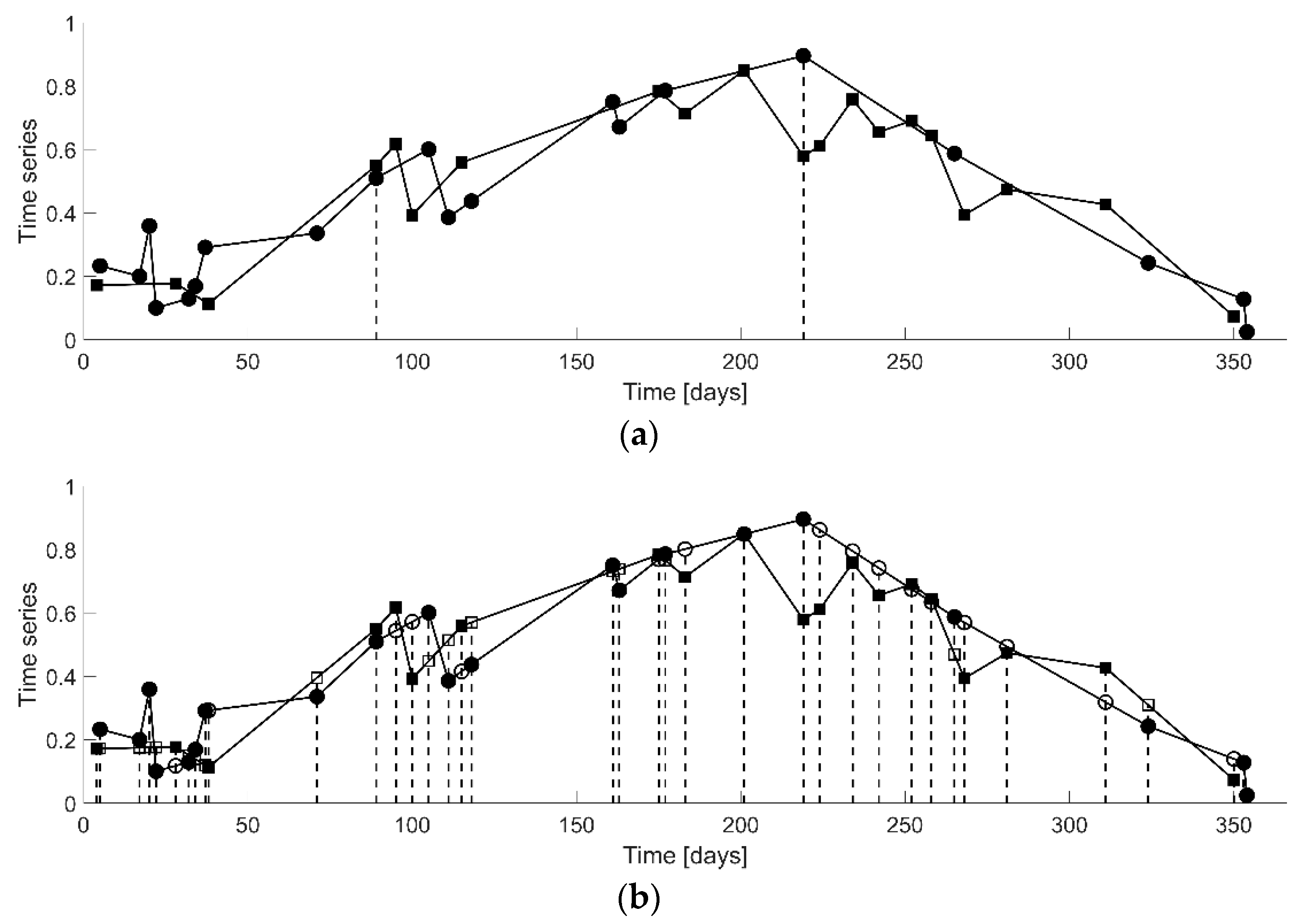
The general situation is thus two time series with $n_1$ and $n_2$ observations with $n_I$ simultaneous observations where $n_I\le \min \left(n_1,n_2\right)$. Figure 2 shows a synthetic example of two time series from two different sources (e.g., two different satellite sensors observed on the same agricultural parcel). In this example, each of the time series has 20 observations out of which only two dates coincide.

As could be seen from the synthetic example of Figure 2, one would typically conclude that the two time series are similar. However, as only two dates coincide, it is not even possible to compute the CC (Figure 2a). In order to circumvent this data issue, we propose to fill the gaps by interpolating each of the time series at the observed dates of the other time series (i.e., the union of the observed dates; Figure 2b). This simple approach has many advantages:

• It is a straightforward generalization of the particular case where all the dates coincide;
• It is simple to implement (a linear interpolation is the simplest solution but others exist, e.g., cubic interpolation or splines);
• It preserves the time dimension of the observations (i.e., values interpolated at new dates directly depend on the proximity to the observed dates);
• It somewhat translates the intuitive visual comparison of the time series (as can be seen in the example of Figure 2).

At this point, it is worth mentioning that the resulting time series do not constitute a genuine sample as some of the values are computed with the interpolation. Consequently, the general formula for the estimation of the variance of the estimation is not valid (i.e., we cannot take the union of the dates as $n$ in the variance formula). There is an equivalent effective size $n^{\prime }$ for the interpolated time series. Several different options were considered for the value of $n^{\prime }$. In the next section, we show, using simulations, that taking

$$n^{\prime }=\min \left(n_1,n_2\right),$$

(7)

(i.e., the number of dates in the shortest time series) is a good empirical rule-of-thumb for substituting the value of $n$ in Equations (4)–(6).

2.3. Comparison of the Methods

For the comparison of the two methods of estimation (i.e., with the simultaneous observations only or with the interpolation), we rely on the observed bias

$$Bia{s}_{\widehat{\rho }}=\frac{1}{N}{\displaystyle \sum }_{i=1}^N\left({\widehat{\rho }}_i-\rho \right),$$

(8)

the observed root mean square error (RMSE)

$$RMS{E}_{\widehat{\rho }}=\sqrt{\frac{1}{N}{\displaystyle \sum }_{i=1}^N{\left({\widehat{\rho }}_i-\rho \right)}^2},$$

(9)

the observed percentage of missing estimation and the observed 95% central interval (i.e., estimated with the empirical quantiles), where $\rho$ is the true CC.

In a second step, we want to verify that the variability is correctly estimated using the definition of $n^{\prime }$ in Equation (7) as a substitute of $n$ in Equations (2)–(6). In particular, we would like to compare this option against two alternatives:

• $\sqrt{n_1{n}_2}$ (i.e., the geometric mean of the observed sample sizes)
• $\left(n_1+n_2\right)/2$ (i.e., the arithmetic mean)

For this purpose, we compute the success rate of the different estimated 95% confidence intervals, i.e., the percentage of times that the true CC is contained in the estimated 95% confidence intervals (see Equation (5)).

In order to have a basis of reference, we also defined a control method that corresponds to the situation where both time series are observed on the union of both extracted sets of dates. As this control method is supposed to be the optimal situation (since the set of observed dates is the largest and there is no interpolation needed), we can build a confusion matrix between the estimated confidence intervals of the control method and the interpolation method with different criteria for $n^{\prime }$. The overall accuracy (OA) can be computed using the number of agreement cases.

3. Results

3.1. Validation using Simulations

The proposed methodology is tested here using simulated time series. The main advantage of simulations is that all the information is known (in our case, the target CC between the two time series) and repeated simulations allow us to derive observed bias and variability of the estimators.

In this test, we relied on a three-step simulation algorithm. First, we simulate two time series over a year (i.e., their length is equal to $N=365$) with two sinusoidal functions and superposed them with white noise. Then, in order to simulate two scarce time series, we randomly select two numbers in the interval [10;20] and assign the values to variables $n_1$ and $n_2$ (i.e., the respective number of observations of the two time series). Finally, both time series are randomly subsampled for variables $n_1$ and $n_2$, which represent a number of observation dates, thus a known sample size for each time series. As the actual observed dates are completely accidental, the number of simultaneous observations varies. We repeat this simulation algorithm 500,000 times. One can prove that this number of simultaneous observations is a random variable following a hypergeometric distribution with $n_1$ draws from $N$ objects with $n_2$ success states. Using the conventions above, there is between 91% and 99% chance that the number of simultaneous observations is strictly smaller than three, which is the worst condition for the estimation of a CC based only on simultaneous dates.

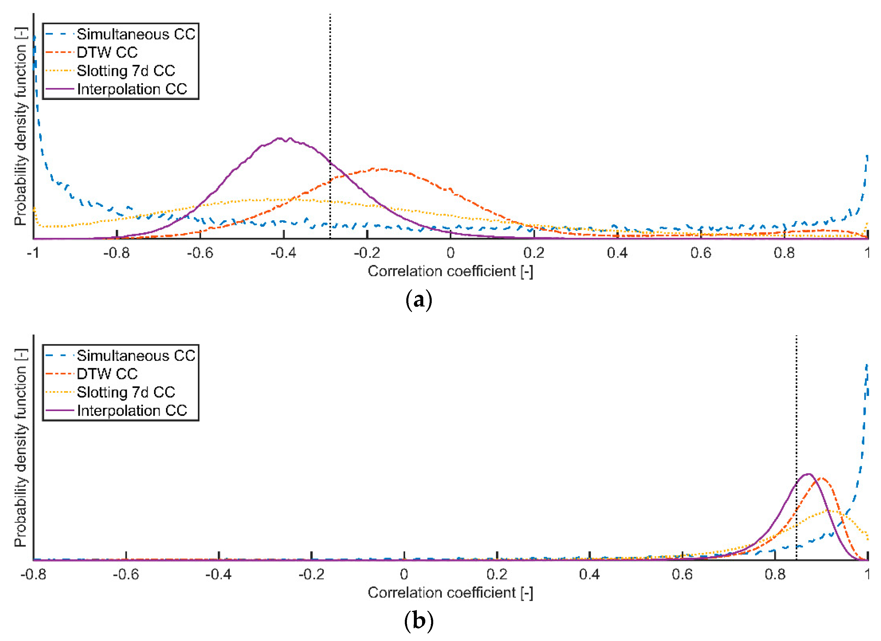
Among the multitude of potential curves, here we show two example cases: (i) with a small negative CC and (ii) with a strong positive CC. For each of the simulated pairs of time series, we estimate five CCs: (i) using the proposed methodology, (ii) using a slotting method with three different bin size (three, seven and 14 days), (iii) DTW with a Sakoe–Chiba band of 45 days (following [8]) and, when possible, using the simultaneous observations only. Figure 3 shows the observed distributions of these estimators. One clearly sees that the proposed method provides better estimations. All the statistics (e.g., the observed bias, the root mean square errors, the estimated quantiles) point in favor of our proposed method (see

Table 1. Descriptive statistics of the CC estimators for the simultaneous observations, the slotting method with three different bin sizes, DTW with a Sakoe–Chiba band of 45 days, and the interpolation method and for both examples.

Method	True Correlation	Bias	RMSE	% Missing Number	95% Central Interval
Simultaneous	–0.29	0.05	0.68	97%	[–0.99;0.99]
Slotting 3d	–0.29	0.04	0.59	19%	[–0.99;0.99]
Slotting 7d	–0.29	0.02	0.42	1%	[–0.94;0.75]
Slotting 14d	–0.29	0.00	0.31	0%	[–0.80;0.41]
DTW 45d	–0.29	0.19	0.37	2%	[–0.57;0.86]
Interpolation	–0.29	–0.09	0.18	0%	[–0.67; –0.04]
Simultaneous	0.85	–0.09	0.43	97%	[–0.73;1.00]
Slotting 3d	0.85	–0.07	0.37	20%	[–0.59;0.99]
Slotting 7d	0.85	–0.04	0.23	1%	[0.22;0.99]
Slotting 14d	0.85	–0.03	0.14	0%	[0.47;0.97]
DTW 45d	0.85	–0.04	0.27	2%	[–0.28;0.96]
Interpolation	0.85	0.00	0.07	0%	[0.68;0.94]

for the details). Finally, as anticipated, the coefficients could be estimated for only 3% of the simulations when using the simultaneous observations only, contrary to the proposed method where a 100% success rate was observed. The success rate of the slotting method lies between those of the simultaneous and our proposed method. Providing a reliable estimation even in extreme cases where the simultaneous observations are scarce is clearly the main advantage of our method.

Besides the estimation of the CCs, we also introduced a method for estimating the precision of the estimator (see Equations (4)–(6) for details). For that purpose, we proposed to substitute $n$ (i.e., the number of paired observations) with $n^{\prime }$, which is the effective sample size. Three alternatives are tested: (i) the minimum of the sample sizes, (ii) the geometric mean of the sample sizes, and (iii) the arithmetic mean of the sample sizes.

As described in Section 2.3, we computed the success rates of the estimated 95% confidence interval for each of the three criteria above (see

Table 2. Comparison of the success rates of the estimated 95% confidence interval for the correlation coefficient and overall accuracy with the control method for the three different criteria of effective sample size $n^{\prime }$.

Criteria for the Value of ${\mathit{n}}^{\prime }$	True Correlation	Success Rate of Control Method	Observed Success Rate	Overall Accuracy with Control Method
$\mathbf{min}\left({\mathit{n}}_{\mathbf{1}},{\mathit{n}}_{\mathbf{2}}\right)$	–0.29	99.48%	98.95%	98.72%
$\sqrt{n_1{n}_2}$	–0.29	99.48%	98.45%	98.33%
$\left(n_1+n_2\right)/2$	–0.29	99.48%	98.40%	98.28%
$\mathbf{min}\left({\mathit{n}}_{\mathbf{1}},{\mathit{n}}_{\mathbf{2}}\right)$	0.85	99.39%	98.56%	98.35%
$\sqrt{n_1{n}_2}$	0.85	99.39%	97.95%	97.86%
$\left(n_1+n_2\right)/2$	0.85	99.39%	97.89%	97.80%

). For each of the three criteria, the success rate was larger than the objective 95%. This indicates that the confidence intervals are larger than expected, hence that each of them overestimate the variability. Such overestimated success rates were also observed for the control method (i.e., where no interpolation was needed). Thus, it does not invalidate the proposed method and the tested criteria for $n^{\prime }$.

As a second metric of comparison, the observed overall accuracy with the control method was slightly larger for the “minimum of the sample sizes” criterion.

3.2. Case Study: NDVI Time Series from Sentinel-2 and PlanetScope on Arable Cropland in The Netherlands

In this section, we show how the proposed method performs on real data.

For the definition of geometric boundaries of agriculture parcels, we used the Geospatial Aid Application (GSAA) dataset information publicly available through The Netherlands open geo-data infrastructure (http://www.nationaalgeoregister.nl). NDVI time series were retrieved from two different image data sources; Sentinel-2 MultiSpectral Instrument (MSI) and PlanetScope imagery. The signal extraction from the Copernicus Sentinel-2 MSI was performed using the product type Level-2A (i.e., bottom atmosphere reflectance) acquired by both twin satellites, Sentinel-2A and Sentinel-2B. As far as the PlanetScope image data is concerned, a comparable product was selected as the analytic ortho scene SR (surface reflectance). In this particular application, we expect a large majority of similarity between pairs of time series since (i) pairs of time series are extracted for the same parcel, (ii) they are extracted over the same period of time, and (iii) Sentinel-2 and PlanetScope products have similar spectral bands.

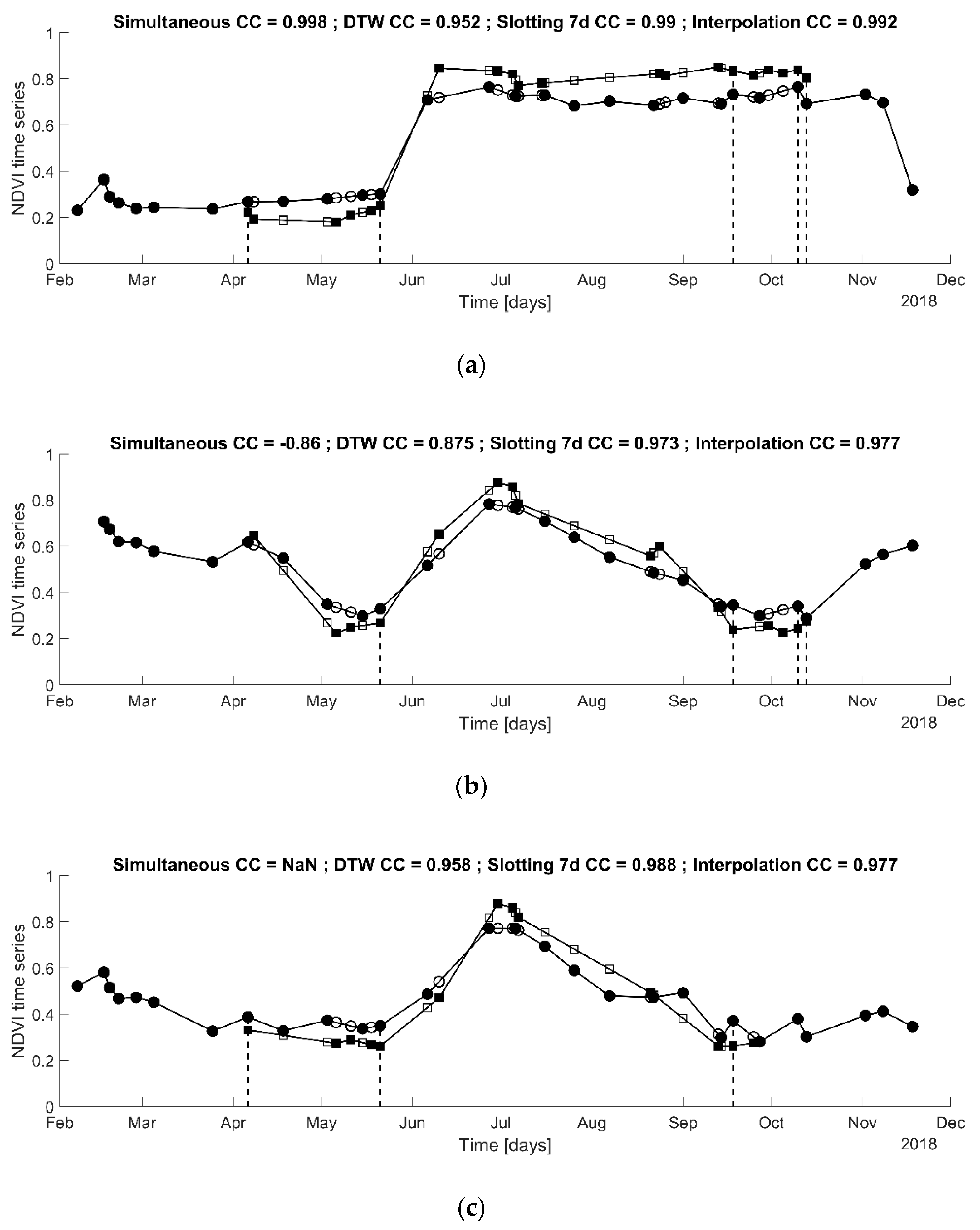
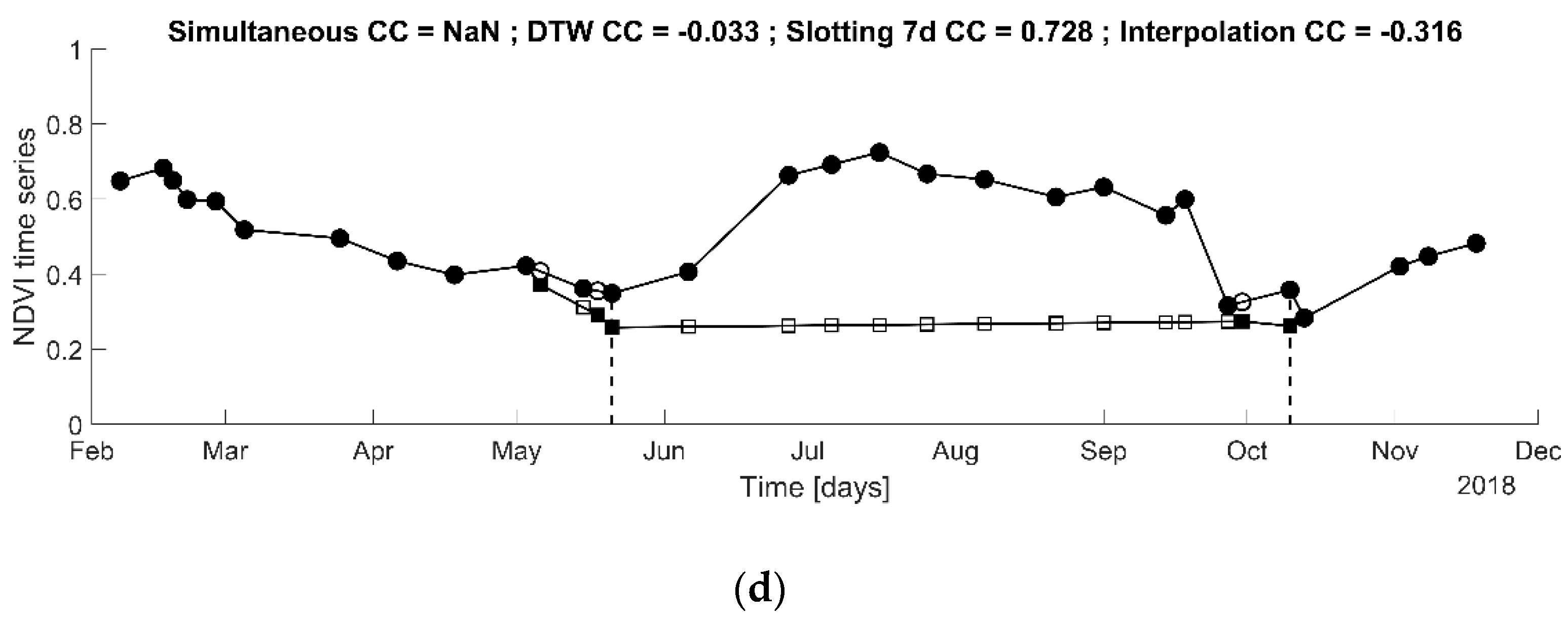
The time series of the 1670 parcels were processed by applying the same estimation methods as for the simulated examples. For the majority of the cases, all the methods performed correctly, having similar results (see Figure 4). However, as expected, the estimation when using the simultaneous observations only could not be computed for 23% of the parcels (see

Table 3. Comparison of the occurrences of missed estimations, of the average and standard deviation of the CCs, and occurrences of accepted hypothesis “$H_0:\rho \le 0.5$” against the alternative hypothesis “$H_1:\rho >0.5$” for the 1670 parcels.

Methods	Not Computed	Average of Correlation Coefficients	Observed Range of Correlation Coefficients	Accepted Tests $“{\mathit{H}}_0:\mathit{\rho }\le 0.5”$ against $“{\mathit{H}}_1:\mathit{\rho }>0.5”$
Simultaneous	385 (23%)	0.87	[–0.91;0.99]	432 (25.9%)
Slotting 3d	16 (0.8%)	0.94	[–0.82;0.99]	83 (5.0%)
Slotting 7d	14 (0.8%)	0.92	[–0.34;0.99]	61 (3.7%)
Slotting 14d	14 (0.8%)	0.87	[–0.48;0.99]	73 (4.4%)
DTW 45d	14 (0.8%)	0.86	[–0.26;0.99]	259 (15.5%)
Interpolation	14 (0.8%)	0.93	[–0.32;0.99]	78 (4.7%)

). For comparison, this occurred for only 0.8% when using the interpolation method. For each of the 14 cases, there were less than three Sentinel-2 images available, thus the CCs could not be computed. On average, when using the interpolation method, the estimated CCs were higher (0.93 against 0.87) and the observed range of the estimations is narrower (minimums are -0.32 versus -0.97). In addition, the statistical test on the hypothesis “$H_0:\rho \le 0.5$” with the alternative hypothesis “$H_1:\rho >0.5$” based on Equation (6) was accepted for only 78 cases when using the interpolation method against 432 when using the simultaneous observations. This shows again that the proposed method circumvents most of the limitations of the classical estimation of the CC.

4. Discussion

The results presented in the previous section show that the proposed method brings significant improvements when comparing severely scarcely sampled time series (i.e., less than 20 acquisition dates). It is based on the idea that gaps between observed dates can be interpolated in order to artificially increase the number of observations. Even though this is a very simple idea, it proved to be both valid and a natural translation of a visual interpretation of the time series. The CCs that were computed using this interpolation method were coherent with their visual interpretation counterparts.

As noted in the synthetic case study, we observed that the constructed 95% confidence intervals actually contained more than 99% of the true simulated CC even when no interpolation was performed (i.e., what we called the control method). However, we also validated in parallel (results not shown here) that Equation (4) is correct for uncorrelated series (i.e., $X_i$ and $Y_i$ are correlated but the $X_i$ and the $Y_i$ are not correlated together). This is a clear indication that the presence of trends in the series tends to decrease the actual variability of the estimated CCs compared to Equation (4). Nevertheless, if this is a limitation, it is related to the use of the CC itself, not on the use of the interpolation strategy. While this brings doubts of the validity of Equation (4) in the context of time series, it does not invalidate our proposed approach. Moreover, since the variability is overestimated, the constructed confidence intervals and equivalent statistical tests are more conservative (i.e., if the null hypothesis “$H_0:\rho \le 0.5$” is rejected, it is very likely that it is a true rejection). In other words, the type I error is smaller than expected. The opposite case of an underestimated variability is riskier because the alternative hypothesis “$H_1:\rho >0.5$” would then be accepted too easily (i.e., we believe that the test is at 95% but it is actually at a smaller percentage).

On the real data example, the estimations were consistently high for the large majority of the parcels. The only cases where the CCs were estimated as small corresponded to obvious lack of data in a crucial period of the crop season, such that no trend could actually be seen in the Sentinel-2 time series. On the contrary, in such conditions, we may expect a lower similarity between the time series because of this lack of information. For instance, in Figure 4, one could argue that the slotting method is actually overestimating the similarity.

The precision of the estimations was also significantly improved. The number of accepted “$H_0:\rho \le 0.5$” hypotheses significantly decreased when using the interpolation method. Indeed, more information were taken into account than merely using the simultaneous observations. The interpolation step translates the temporal evolution of the time series more adequately. The slotting method also showed some advantages, but it requires at least 20 observations in order to perform correctly. The DTW was able to bring some improvements but not as much as the slotting or interpolation methods.

Finally, the proposed interpolation method proved to be very efficient against the lack of simultaneous observations between the two time series. In the Dutch example, we observed a quasi disappearance of the cases where the CCs could not be computed (from 385 to only 14). This is a clear benefit of the proposed method since it drastically reduces the number of undecided cases (i.e., where there is not enough information for a conclusion). The slotting method proved to be an alternative but the results highly depend on the density and spread of the acquisition dates and on the bin size. Comparatively, the interpolation approach correctly brings added temporal information and helps fill the sampling gaps without requiring any parameters. Clearly, this benefit is less obvious for long time series observed on a regular time step with few missing data.

5. Conclusions

In this paper, we presented a simple method to quantify the similarity between scarce remotely sensed time series. The index is based on the Pearson’s correlation coefficient (CC) between the two time series. As we are interested in the similarity between the time series, the CC is computed on the raw time series (i.e., without removing the trends). The use of an interpolation step enables us to circumvent the issue of the scarcity of the time series. The theory of CC estimation was also extended to the estimation based on a mix between genuine observations and interpolated values.

The proposed method was tested both on simulated and real application data. It proved to be very efficient and specifically useful when the number of simultaneous observations is limited. Indeed, in such conditions, neither the cross- and autocorrelation functions nor a simple CC between the true pairs of observations can be accurately estimated. In many cases, the estimator cannot be computed at all. Limiting the computation to the zero-lag bin of the cross-correlation function is a possible alternative but at the cost of larger bin sizes, which might risk diluting the actual similarity with dissimilar pairs of observations. On the contrary, the interpolation step adequately brought the temporal information in order to cope with both the temporal gaps and the lack of simultaneous observations.

In our context, the objective was to evaluate the similarity between two time series for which the CC is a sufficient quantitative index. However, one could also extend the analysis to more complex indexes. After the same interpolation step, one can generalize the approach by replacing the CC with other types of indexes such as Spearman’s rho or Kendall’s tau [15], an index of agreement [10], or mutual information [16]. This approach thus opens interesting avenues for the analysis of scarce remotely sensed time series.

References

- Box, G.E.P.; Jenkins, G.M. Time Series Analysis: Forecasting and Control, 2nd ed.; Holden-Day: San Francisco, CA, USA, 1970. [Google Scholar]
- Löw, F.; Duveiller, G. Defining the spatial resolution requirements for crop identification using optimal remote sensing. Remote Sens. 2014, 6, 9034–9063. [Google Scholar] [CrossRef]
- Di Salvo, A.; Faggioli, L.; Morelli, B. Orbit selection criteria for optical dual-use earth observation satellites. In Proceedings of the 63rd International Astronautical Congress. IAC 2012, Naples, Italy, 1–5 October 2012; pp. 5651–5661. [Google Scholar]
- Cressie, N. Statistics for Spatial Data, Revised ed.; John Wiley and Sons, Inc.: New York, NY, USA, 1993. [Google Scholar]
- Broersen, P.M.T.; Bos, R. Estimating time-series models from irregularly spaced data. IEEE Trans. Instrum. Meas. 2006, 55, 1124–1131. [Google Scholar] [CrossRef]
- Journel, A.G.; Huijbregts, C.J. Mining Geostatistics; Academic Press: London, UK, 1978; p. 194. [Google Scholar]
- Sakoe, H.; Chiba, S. Dynamic Programming Algorithm Optimization for Spoken Word Recognition. IEEE Trans. Acoust. 1978, 26, 43–49. [Google Scholar] [CrossRef]
- Csillik, O.; Belgiu, M.; Asner, G.P.; Kelly, M. Object-based time-constrained dynamic time warping classification of crops using Sentinel-2. Remote Sens. 2019, 11, 1257. [Google Scholar] [CrossRef]
- Maus, V.; Câmara, G.; Cartaxo, R.; Sanchez, A.; Ramos, F.M.; de Queiroz, G.R. A time-weighted dynamic time warping method for land-use and land-cover mapping. IEEE J. Sel. Top. Appl. Earth Obs. Remote Sens. 2016, 9, 3729–3739. [Google Scholar] [CrossRef]
- Duveiller, G.; Fasbender, D.; Meroni, M. Revisiting the concept of a symmetric index of agreement for continuous datasets. Sci. Rep. 2016, 6, 19401. [Google Scholar] [CrossRef] [PubMed]
- Willmott, C.J. On the validation of models. Phys. Geogr. 1981, 2, 184–194. [Google Scholar] [CrossRef]
- Mielke, P. Meteorological applications of permutation techniques based on distance functions. In Handbook of Statistics; Krishnaiah, P., Sen, P., Eds.; Elsevier Science Publishers: New York, NY, USA, 1984; Volume 6, pp. 813–830. [Google Scholar]
- Trauth, M.H. MATLAB® Recipes for Earth Sciences, 4th ed.; Springer-Verlag: Berlin/Heidelberg, Germany, 2005; p. 172. [Google Scholar]
- Fisher, R.A. Statistical Methods for Research Workers, 9th ed.; Oliver and Boyd Ltd.: Edinburgh, UK, 1944; pp. 192–193. [Google Scholar]
- Liu, C.; Frazier, P.; Kumar, L. Comparative assessment of the measures of thematic classification accuracy. Remote Sens. Environ. 2007, 107, 606–616. [Google Scholar] [CrossRef]
- Hong, T.; Hart, K.; Soh, L.-K.; Samal, A. Using spatial data support for reducing uncertainty in geospatial applications. GeoInformatica 2014, 18, 63–92. [Google Scholar] [CrossRef]
© 2019 by the authors. Licensee MDPI, Basel, Switzerland. This article is an open access article distributed under the terms and conditions of the Creative Commons Attribution (CC BY) license (http://creativecommons.org/licenses/by/4.0/).