Phenology and Seasonal Ecosystem Productivity in an Amazonian Floodplain Forest

Abstract

Several studies have explored the linkages between phenology and ecosystem productivity across the Amazon basin. However, few studies have focused on flooded forests, which correspond to c.a. 14% of the basin. In this study, we assessed the seasonality of ecosystem productivity (gross primary productivity, GPP) from eddy covariance measurements, environmental drivers and phenological patterns obtained from the field (leaf litter mass) and satellite measurements (enhanced vegetation index (EVI) from the Moderate Resolution Imaging Spectroradiometer/multi-angle implementation correction (MODIS/MAIAC)) in an Amazonian floodplain forest. We found that ecosystem productivity is limited by soil moisture in two different ways. During the flooded period, the excess of water limits GPP (Spearman’s correlation; rho = −0.22), while during non-flooded months, GPP is positively associated with soil moisture (rho = 0.34). However, GPP is maximized when cumulative water deficit (CWD) increases (rho = 0.81), indicating that GPP is dependent on the amount of water available. EVI was positively associated with leaf litter mass (Pearson’s correlation; r = 0.55) and with GPP (r = 0.50), suggesting a coupling between new leaf production and the phenology of photosynthetic capacity, decreasing both at the peak of the flooded period and at the end of the dry season. EVI was able to describe the inter-annual variations on forest responses to environmental drivers, which have changed during an observed El Niño-Southern Oscillation (ENSO) year (2015/2016).

1. Introduction

Tropical forests are known for their high productivity, accounting for 33% of terrestrial net primary production, which regulates carbon-climate feedbacks [1]. In this context, the Amazon forest represents a sink of 0.42 to 0.65 Pg C per year of total carbon assimilated, making it the most significant carbon sink on the planet [2]. However, extreme droughts have demonstrated the sensitivity of this ecosystem to environmental changes. Previous studies have reported aboveground biomass loss, increased tree mortality [3,4] and a long-term decreasing trend of carbon accumulation [5], which could lead to the possible shift of forest functioning from a sink to a source of CO₂ during long-term droughts [6,7].

Although detailed knowledge about the tropical forest carbon cycle is still lacking, previous studies have sought to understand the mechanisms of seasonal photosynthesis control, such as water and light availability [8,9] and phenological cycles [10,11,12]. To understand these seasonal patterns on a larger scale, several studies have correlated seasonal environmental drivers with remote sensing-based multispectral vegetation indices in the Amazon basin. Some of them have suggested the Amazon rainforest is resilient to seasonal droughts [13] and extreme droughts [14]. Other studies, however, reported that an apparent greening of the forest canopy could be attributed to abnormal leaf flushing or as an effect of sun position in relation to the sensor, increasing near infrared reflectance, and thus not reflecting a true resilience from the forest [15,16,17,18,19,20]. Part of these uncertainties has been attributed to the high atmospheric contamination of the MODIS (Moderate Resolution Imaging Spectroradiometer) sensor surface reflectance data, the most commonly used sensor for phenological studies in the tropics [21,22].

Given the reported uncertainties related to sun-sensor geometry effects and atmospheric contamination, progress has been made towards the development of more robust atmospheric correction methods and data normalization procedures for MODIS data, such as the multi-angle implementation correction (MAIAC) algorithm [23] implementation of the bidirectional reflectance distribution function (BRDF). Enhanced vegetation index (EVI) values extracted from this improved MODIS product (MODIS-MAIAC) have shown a correlation between phenology and productivity of the Amazon forest [11,24,25,26,27].

Apart from these advances, a remaining limitation is that the majority of studied forest plots in the Amazon are located in terra firme (upland) forests, even though c.a. 14% of the basin is covered by flooded forests [28], which remain understudied. These ecosystems are subjected to seasonal, long-lasting and monomodal flood pulses [29], with studies reporting adaptation mechanisms developed by species in these environments in response to the excess or lack of water. During the flooded period, some species can increase root porosity, release biological volatile organic compounds into the atmosphere, enrich the rhizosphere with oxygen, reduce photosynthesis and exhibit anaerobic metabolism [30,31]. During the dry season, decreases in leaf water potential, foliar surface, and xylem flow have been observed, which reduce water loss through transpiration [32].

Floodplain areas are widely recognized for the ecosystem services they provide, playing an important role in water and climate regulation services [29,33]. Different studies have pointed to a higher resilience of Amazonian floodplain forests to seasonal droughts [31,34,35], as during the terrestrial phase, these forests had higher rates of stem growth [34] and greater rates of CO₂ assimilation as a result of new leaves and soil aeration [32,36]. Conversely, a period of dormancy has been suggested to be a survival strategy during the aquatic phase [34].

According to the most recent IPCC report, floodplain forests are one of the most threatened ecosystems because of the undergoing “savannization” feedback to extreme drought events [37]. In this scenario, the carbon and methane sink services they provide could be compromised [38]. Furthermore, recent reports have demonstrated considerable tree mortality on central Amazonian floodplains due to changes in flooding quota by upstream dam construction [39]. Although induced by indirect changes to the flood pulse, direct effects of extreme droughts also revealed the sensibility of this ecosystem. The droughts of 1997 and 2005 have also shown that fires have a stronger and longer-lasting impact on floodplain forest structure than in upland forests; moreover, these floodable areas are located at the core of the Amazon forest, threatening the resilience of the entire system [40].

Most Amazonian floodplain studies have been located in the central Amazon basin, surrounding the Solimões and Amazonas rivers. Nonetheless, a different pattern of climate change is expected to occur at the southern portions of the basin, with an increase in temperature and decrease of precipitation during wet seasons [41]. In the southeast region, bordering the Amazon basin, there is an LBA (large-scale biosphere-atmosphere) eddy flux tower site (Bananal site) located on a seasonal floodplain forest, at the transition between the Amazon and Cerrado biomes. Previous studies have suggested that this forest shows two periods of water stress—one due to excess of water in the peak of the rainy season—and another due to water deficit, at the end of the dry season [42,43,44]. During the El Niño drought of 2005, decreased rates of evapotranspiration [42] and increasing rates of tree mortality were reported in this region [44].

Given the uncertainties of floodplain environmental response to seasonal cycles of flood and dry periods, this study aims to evaluate the seasonal productivity of this floodplain forest located in the Amazon-Cerrado transition, as well as its environmental controls, based on field observations and on enhanced vegetation index (EVI) derived from MODIS (MAIAC) surface reflectance data. We asked the following questions: (i) How does the Bananal seasonally flooded tropical forest respond to flood and drought cycles in terms of evaporative fluxes and gross primary productivity (GPP)? (ii) Do phenological patterns observed from field data agree with landscape-level remote observations (EVI from MODIS/MAIAC)? (iii) Does flooding affect the EVI signal of these forests?

2. Materials and Methods

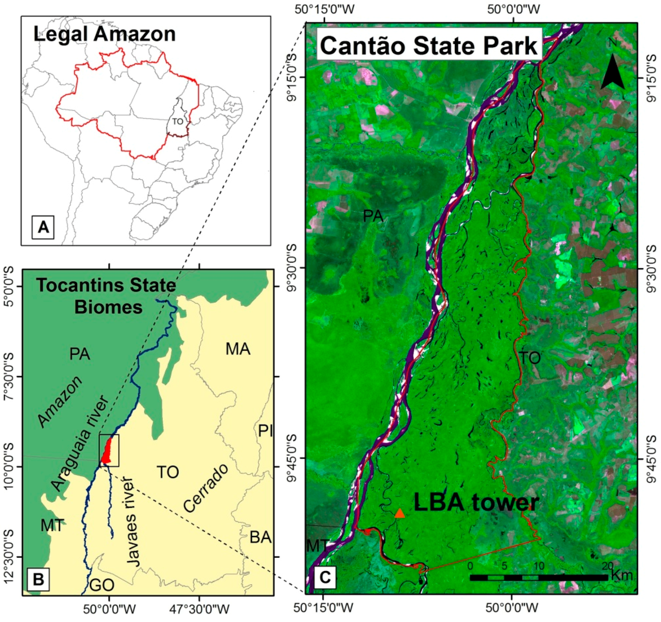
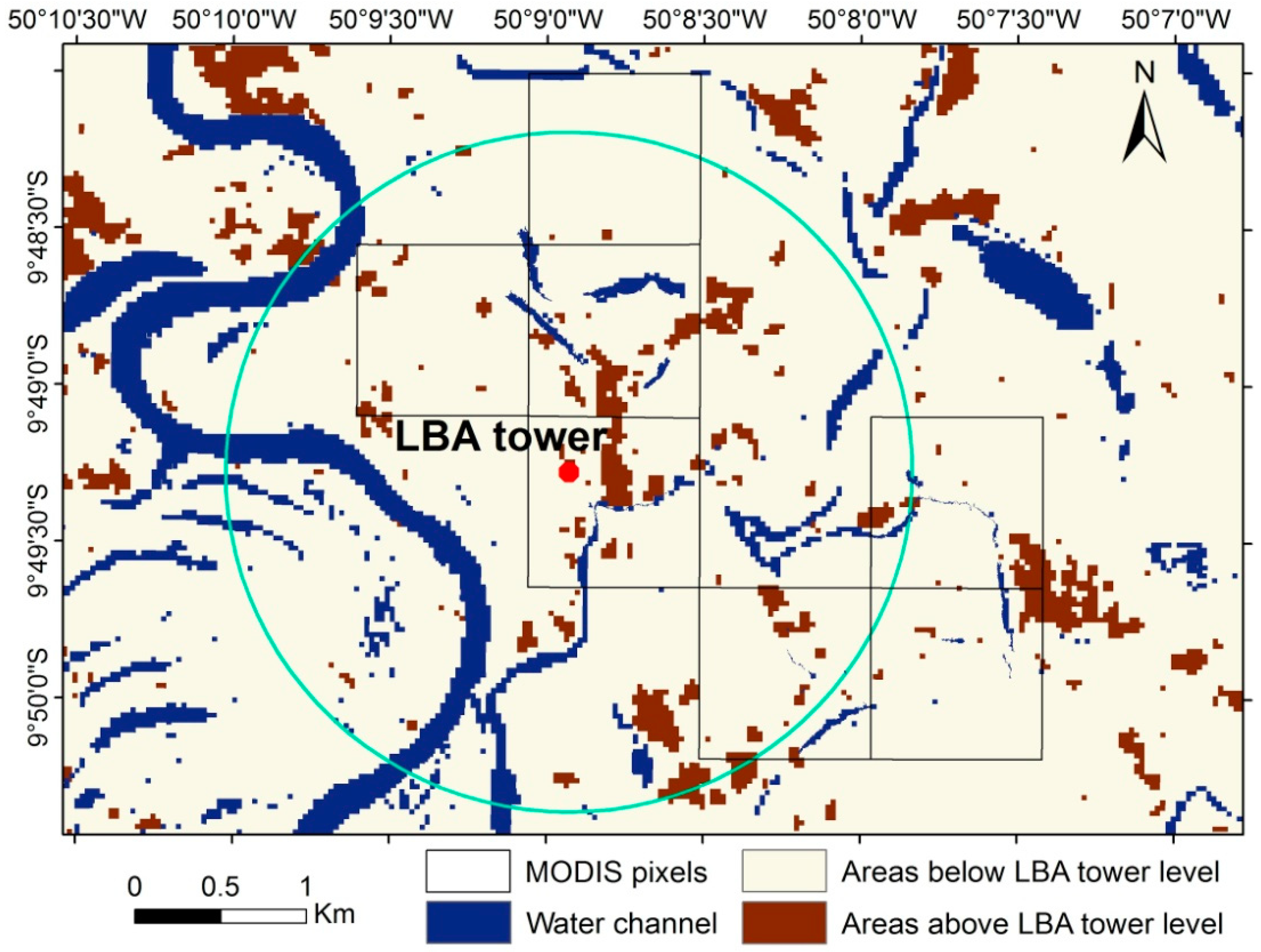
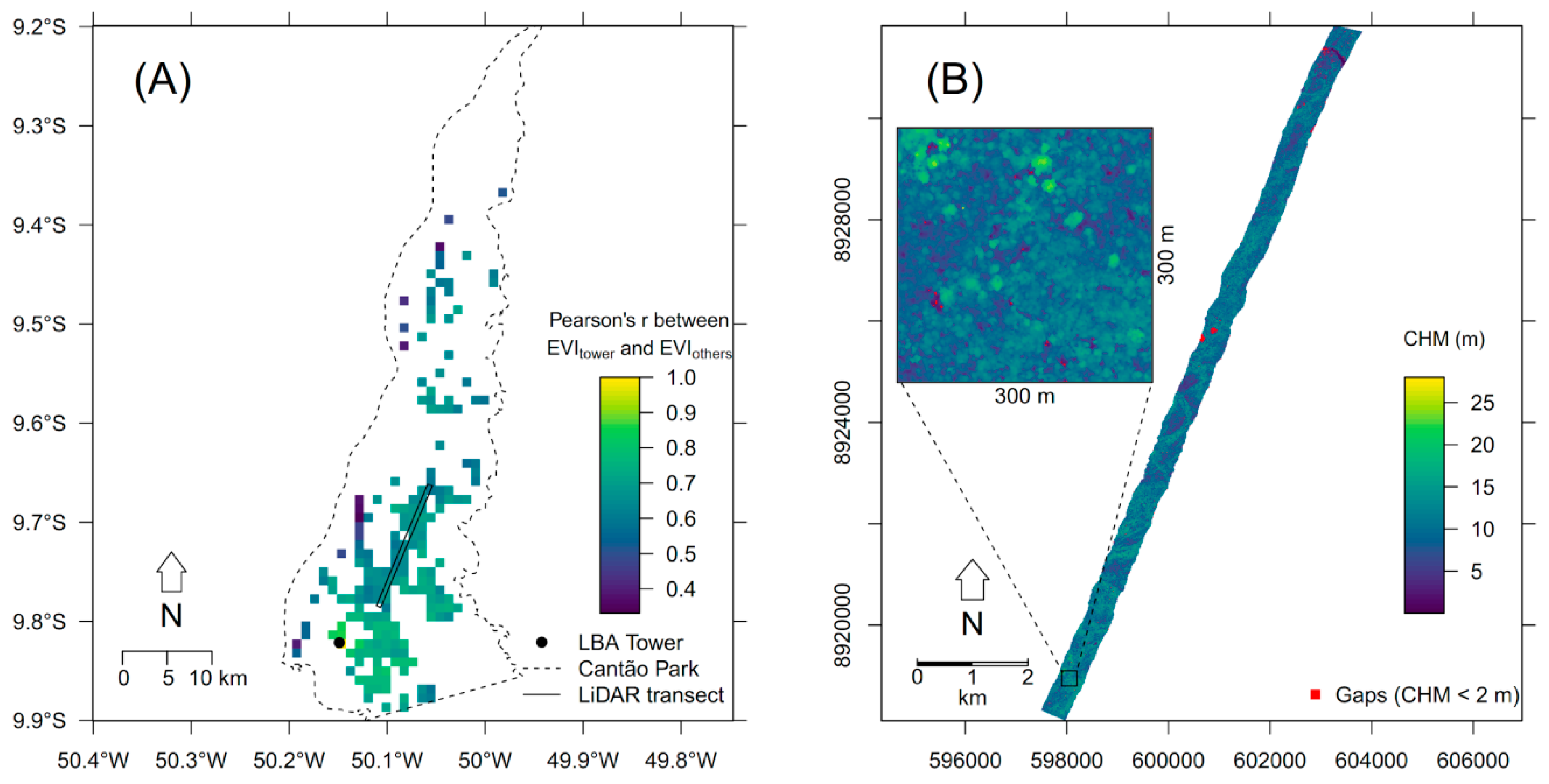
2.1. Study Site

The study site is located in a floodplain area of Cantão State Park (PEC), which consists of approximately 90% natural vegetation and is located about 260 km west of Palmas, state of Tocantins, Brazil (Figure 1). The area is located at the transition between the Amazon and Cerrado (savanna) biomes, bounded in the southwest by the Bananal Island region, which is the largest river island in the world [42]. The LBA micrometeorological tower (Bananal (BAN) site) is located about 2 km east of Javaezinho river, a tributary of Javaes river. The climate is wet-dry tropical, classified “Aw” in Koppen’s climatic classification. The annual rainfall typically varies between 1300 to 1900 mm, and temperature varies from 22 °C in January to 31 °C in September [43]. Dry seasons occur between May and September, and wet seasons between October and April, concentrating approximately 90% of annual precipitation. The local topography is flat and the predominant soil type in this region is Gleysol (Food and Agriculture Organization (FAO) classification) [45].

2.2. Flux Tower and Field Data

Data from the flux tower have been recorded daily since October 2003 and include the following variables: GPP (μmol CO₂ m⁻² s⁻¹), air temperature (Ta, °C), rainfall (mm), net radiation (Rn, in w m⁻²), latent heat (LE, in w m⁻²), specific humidity (q, g Kg⁻¹), pressure (press, kPa) and vapour pressure deficit (VPD, kPa). A detailed description of the methods used in eddy covariance technique the CO₂ ecosystem exchange at this site is reported in Restrepo-Coupe et al. [8] and Costa [43].

Evapotranspiration was calculated from LE and Ta as a function of latent heat of water vaporization (λ) (Equation (1)).

ET = LE ∗ λ,
where λ (J kg⁻¹) = 10³ ∗ (2500 − 2.37 ∗ Ta)

(1)

Vapour Pressure Deficit was calculated through Bolton (1980) equations using a script available freely for the R language (LeBauer, D. 2018). The input parameters are air temperature, specific humidity, and pressure.

Soil moisture has been measured close to the tower using FDR (frequency domain reflectometer) probes installed at four depths 0.2, 0.4, 0.8, and 1.5 m from 2004 to 2006 and from 2006 onwards, two more probes were added at 2.0 and 2.9 m depths.

The Javaes river level record of the Barreira da Cruz station was obtained from the Agência Nacional de Águas (ANA) in Brazil (http://hidroweb.ana.gov.br), from 1990 to 2017. The river level describes the flood pulse and the flood height measured at the tower base (r = 0.76, p < 0.05) (Figure S1).

Gap Filling of CO₂ Estimates

We performed gap filling on night and daily CO₂ estimates according to the method described in Restrepo-Coupe et al. [8]. There was an underestimation of night positive CO₂ fluxes due to insufficient turbulent mixing. We filled each missing nighttime value from an average of all valid nighttime values (from 6 pm to 5 am) within a 5-day window. The data was replaced by the average of this 5-day window, and when this was not possible we applied windows varying 11–31 days. The correction performed in this paper involved 35% of the total night data for a friction velocity (u*) threshold of 0.19 m s⁻¹ for the rainy season and 0.17 m s⁻¹ for the dry season. Our data can be considered below the thresholds and percentage of gaps found in the literature for other sites in the Amazon region [46].

The relationship between photosynthetically active radiation (PAR) and the observed data of NEE (net ecosystem exchange) was used for filling daytime NEE (NEE, assumed as a proxy for turbulent flux) [47,48]. The hyperbolic relationship pattern between these variables included coefficients which represented the maximum photosynthetic efficiency of the canopy (a2), its yield (a3) and the mean ecosystem nocturnal respiration (a1) [48], as described in Equation (2).

$$NEE=a1+\frac{a2\ast PAR}{a3+PAR}$$

(2)

NEE values for PAR < 40 μmol CO₂ m⁻² s⁻¹ were excluded from this analysis since this condition is generally associated with invalid turbulence and abrupt changes in light levels [48]. Further details are described in Restrepo et al. [8].

2.3. Litterfall Collection

Litter was collected in traps installed along a transect of 200 × 800 m near the flux tower, spaced 25 m from each other. From April 2004 to May 2005, litterfall was collected every month from 30 litter traps, with 1 m² size. Litter was sorted into leaf material, reproductive material (flowers and fruits), woody material (twigs), and non-identifiable plant material. Following separation, the material was then dried to a constant mass in an oven and weighed to calculate biomass [49].

2.4. Remote-Sensing Data and Products

We acquired the MODIS-MAIAC product EVI for the study area from the time period of 2004 to 2017 [50]. In this product, prior to EVI calculation, the surface reflectance data were normalized to nadir target and 45-degree solar zenith angle through the Bidirectional Reflectance Distribution function, at a spatial resolution of 1 km and aggregated to biweekly (16-day) composites using the median values. The EVI was calculated using Equation 3 [13]. Further information on image processing and correction are described in Dalagnol et al. [50,51]. The composites were retrieved considering only cloud-free and low atmospheric turbidity according to MAIAC quality flags. For the MODIS-MAIAC pixel containing the flux tower, the mean number of samples per 16-day composite was 4.6 samples for the flooding period (February–May) and 12 samples for the non-flooding period.

$$EVI=2.5\ast \frac{\rho NIR-\rho Red}{\rho NIR+(6\ast \rho Red-7.5\ast \rho Blue)+1}$$

(3)

where ρNIR is infrared reflectance, ρRed is red reflectance, and ρBlue is blue reflectance. The constants (6, 7.5, 1, and 2.5) in the divisor represent the aerosol coefficient adjustment of the atmosphere for the red and blue band, the adjustment factor for the soil and the gain factor, respectively [52].

There is a high density of water channels in the study area. Therefore pixels composed of more than 10% of permanent water were excluded from the analysis, using the Global Forest Change product v1.4 mask [53]. This procedure also eliminated areas that were disturbed between 2000 to 2016. The mask was resampled from 30 m to 1 km according to MODIS pixels resolution. Only pixels around the tower footprint (2 km) meeting these criteria were selected for analysis. To further check the presence of water channels in these pixels, we used the high resolution Bing Virtual Earth image on QGIS 2.18 to visual interpret and manually delineate permanent water bodies, and we found more than 94% of forest cover (Figure S2 and Table S1).

To explore rainfall variability over the time series, we obtained rainfall data from the Tropical Rainfall Measuring Mission (TRMM). This data showed a significant correlation with tower measurements from 2004 to 2014 (r = 0.62, p < 0.001) (Figure S3). We did not use the field measured rainfall data directly due to gaps on records from 2014 to 2016. We also used 2 meter air temperature and vapour pressure deficit data from the ERA5 climate reanalysis [54] to build an inter-annual analysis, due to gaps in tower for these variables from 2010 to 2016. Both variables from the ERA5 reanalysis product had a very high correlation (Ta: r = 0.83, p < 0.001; VPD: r = 0.95, p < 0.001) with tower data (Figures S4 and S5).

The cumulative water deficit (CWD) was calculated to investigate negative monthly precipitation anomalies [55]. We calculated the monthly average ET from the tower, based on records with a good density of observations from 2004 to 2014 (Table S3), since there were gaps in measurements from 2010 to 2016. The CWD increases in magnitude when rainfall is lower than ET. The following rule was applied to the rainfall data (R) for each month (m) with evapotranspiration (E) set at 100 mm month (Equation (4)).

CWD_m = CWD_m−1 + R_m − E_m
If CWD_m > 0 then CWD_m = 0

(4)

We also performed a canopy gap analysis for the studied forests using airborne LiDAR data to assert the degree of expected interference of free standing water under the canopy during the flooded period on MODIS EVI values. The data was collected on 20 February 2016 along a 15 km transect with 500 m width, using a Riegl LMS-Q680i laser scanner at 500 m average flight altitude, 45° fiLMS of view, and 300 kHz scanning frequency. The data had a high pulse density of greater than 5 points per m². Using the point cloud, we derived a canopy height model (CHM) utilizing the highest height of return within 1 × 1 m cells using standard procedures, as described in [56]. We detected canopy gaps following the procedures described in Hunter et al. [56] and considering the traditional Brokaw’s gap definition of a hole in the forest that extends to at least 2 meters above the ground. Lidar data from this study was obtained by the EBA project (Amazon biomass estimate, EBA). Regarding the canopy structure, as this transect is located 7 km away from the LBA tower, we compared tree heights of 170 individuals distributed in two experimental plots located 200 (BAN1) and 100 meters (BAN2) from the tower [57] with LiDAR measurements. A forest inventory was performed in 2015 in these plots and tree heights were measured with a telescope pole of 15 m length (Table S2).

2.5. Statistical Analysis

The seasonal cycle of climatic drivers (rainfall, soil moisture, flood amplitude, evapotranspiration, net radiation, deficit vapour pressure, cumulative water deficit and air temperature) and phenology from EVI were based on monthly mean measurements from 2004 to 2016, while the GPP monthly average was based on measurements from 2011 to 2013 due to data availability (Figure S6). The analyzed EVI was based on the mean value of the seven pixels around the tower, considering the limits of the flux tower footprint and filtering of forest cover areas (>90%).

Since there are many parameters measured from different sources, we summarized data acquisition, availability and usage on

Table 1. Availability and usage description of tower, satellite and field data.

Parameter	Acquisitions	Start Year	End Year	Usage
LE	Tower	2004	2014	ET computation
PAR	Tower	2011	2013	NEE computation
Press	Tower	2004	2014	Relative humidity (RH) computation
q	Tower	2004	2016	RH and VPD computation
Rn	Tower	2004	2014	Correlation variable
GPP	Tower	2011	2013	Productivity estimate/Correlation variable
ET	Tower	2004	2014	Correlation variable
VPD	Tower/Satellite	2004	2016	Correlation variable
Ta	Tower/Satellite	2004	2016	VPD and ET computation/Correlation variable
Rainfall/TRMM	Tower/Satellite	2004	2014	Correlation variable
CWD	Tower/Satellite	2004	2016	Correlation variable
EVI	Satellite	2004	2016	Phenology and productivity proxy/Correlation variable
Soil moisture	Field	2014	2016	Correlation variable
Litterfall	Field	2004	2005	Phenology proxy/Correlation variable
Flood height	Tower	2004	2016	Define seasonal flooding

.

We divided our seasonal analyses into two distinct periods: Flooded (Feb to May) and non-flooded (Jun to Jan). The phenology pattern described by EVI was also analyzed with ground data (litterfall) from 2004 to 2005 [49]. We also performed an inter-annual analysis, in order to evaluate anomalies in relationships from year to year between monthly EVI and the climatological variables described in Table 1.

We performed correlation tests using daily data from 2011 to 2013 (GPP data availability) to measure the degree of association between GPP and the climatic variables estimated for the significant models (p-value ≤ 0.05). We used the Shapiro–Wilk test to analyze the normality of the distributions of all variables described in Table 1. We performed the Pearson correlation test (r) between GPP, monthly EVI, and leaf litter mass (normally distributed variables). Other variables (rainfall, net radiation, evapotranspiration, soil moisture, CWD, temperature and vapour pressure deficit) were not normally distributed, thus we used the non-parametric Spearman’s correlation (rho) to measure the degree of association between them with daily and monthly GPP.

3. Results

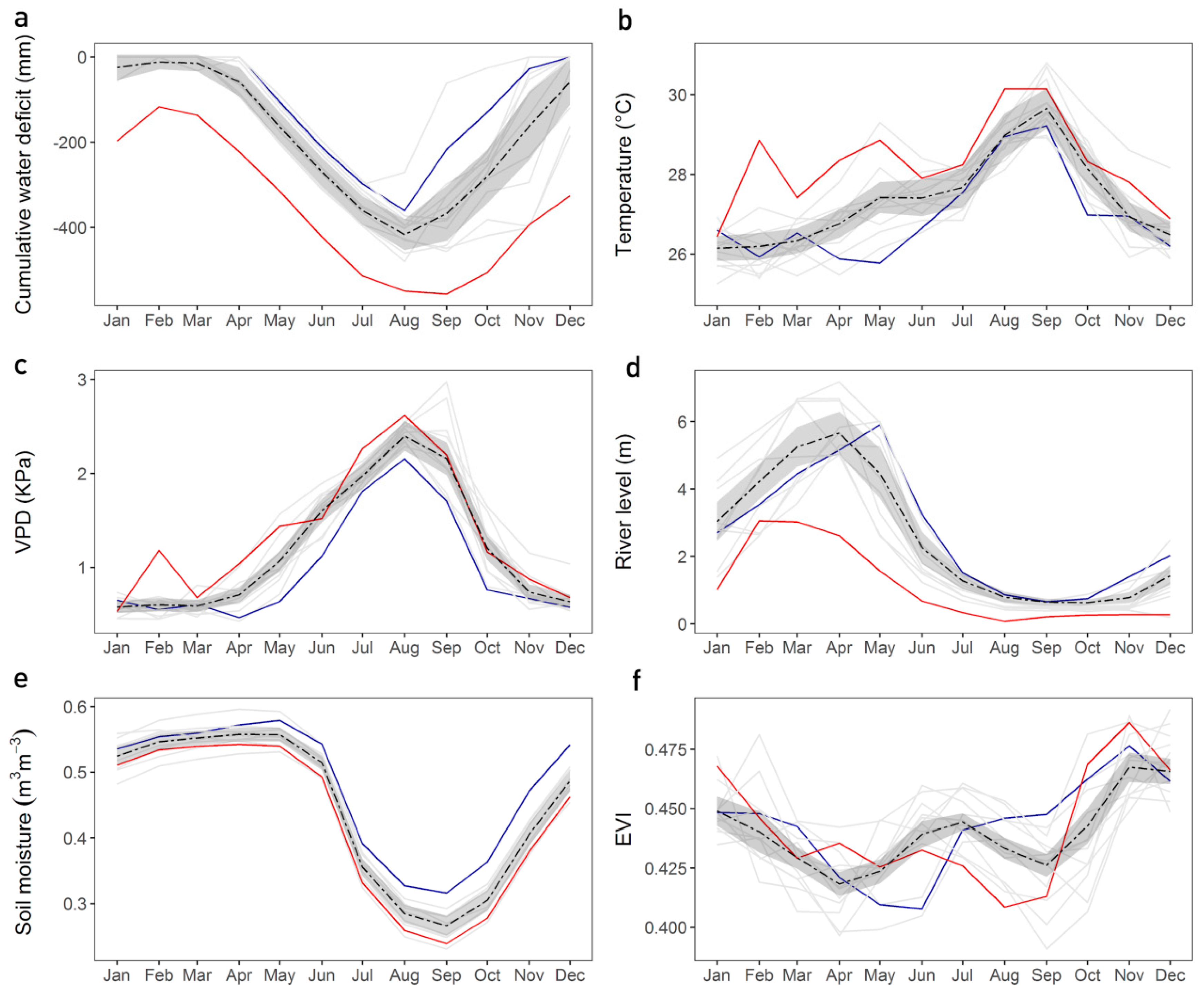
3.1. Seasonal Meteorological, Gross Primary Productivity (GPP) and Enhanced Vegetation Index (EVI) Patterns

The seasonal variation of GPP and its interaction with environmental drivers (rainfall, evapotranspiration, cumulative water deficit, vapour pressure deficit, soil moisture, net radiation and temperature) and phenology (described through EVI), showed different patterns among periods of the year. We observed an extended dry season from May to September, when rainfall was below 100 mm·month⁻¹, while ET remained high through all seasons (mean of 110 mm·month⁻¹), especially during the flooding (Figure 2a). This high ET values indicated that soil moisture was sufficient to attend the atmospheric demands, which were described by the increased VPD (Figure 2c) and decreased CWD from April to August (Figure 2b).

Although ET at this site exhibited a flat pattern, slight maximum values coincided with maximum GPP (Figure 2f), but the first and more pronounced peak occurred in March (123 mm), mid-flooding, in response to an increase of Rn at this month (Figure 2e). The second peak occurred in June/July (116 mm), mid-dry season, and a third in December, mid rainy season (122 mm), before the period of flooding.

Net radiation did not seem to be the main productivity driver on this site, since during the months of highest GPP values (June and December), Rn varied between 276 and 282 W·m², respectively, and not close to the maximum value of 314 W·m² in August (Figure 2e).

Soil moisture seems to be the main productivity driver at this forest (Figure 2d). Soil water content remained relatively constant from March to June, especially for layers at 20 cm, 40 cm, 80 cm, and 200 cm depth, indicating that the soil was 100% saturated. Layers at both 150 cm and 293 cm depth remained saturated for a longer time, extending until July and August, respectively. During the months of maximum GPP (June and December), the mean soil moisture of layers at 20 cm, 40 cm, 80 cm, and 200 cm were 0.541 and 0.501 m³ m⁻³. Conversely, in April and August (months of minimum GPP), the average volumetric soil moisture content was 0.585 and 0.344 m³ m⁻³, respectively. Thus, we observed that both flooding and dry soil limited productivity at the BAN site.

EVI values (Figure 2g) indicated a bimodal pattern of foliar production, with a peak in July (mid-dry season) and a more pronounced peak in December (mid-rainy season prior to flooding). These EVI peaks were in phase with GPP, which decreased at the peak of flooding (April) and at the peak of the dry season (September).

GPP remained high during the flooded period (Figure 2f) due to the shorter duration of soil saturation in higher terrain portions concentrated near the flux tower (Figure 3). Therefore, the mean flood amplitude of 1.3 m (Figure 2d) could take longer to saturate the soil at the beginning of the flooded period. Similarly, these terrain portions would be aerated first at the end of flooding, enabling photosynthesis to recover after the anoxic conditions that occur during the flooded period, explaining the GPP increase in May, before the end of the flooded period (Figure 2f). However, the majority of the terrain around the tower footprint (89%) is at the same level or below the base tower level. This might be the reason why the landscape remained under anoxic conditions for a longer time, which was reflected on canopy response, suggesting a one-month lag between EVI and GPP during non-flooded months, from May to September (Figure 2f,g).

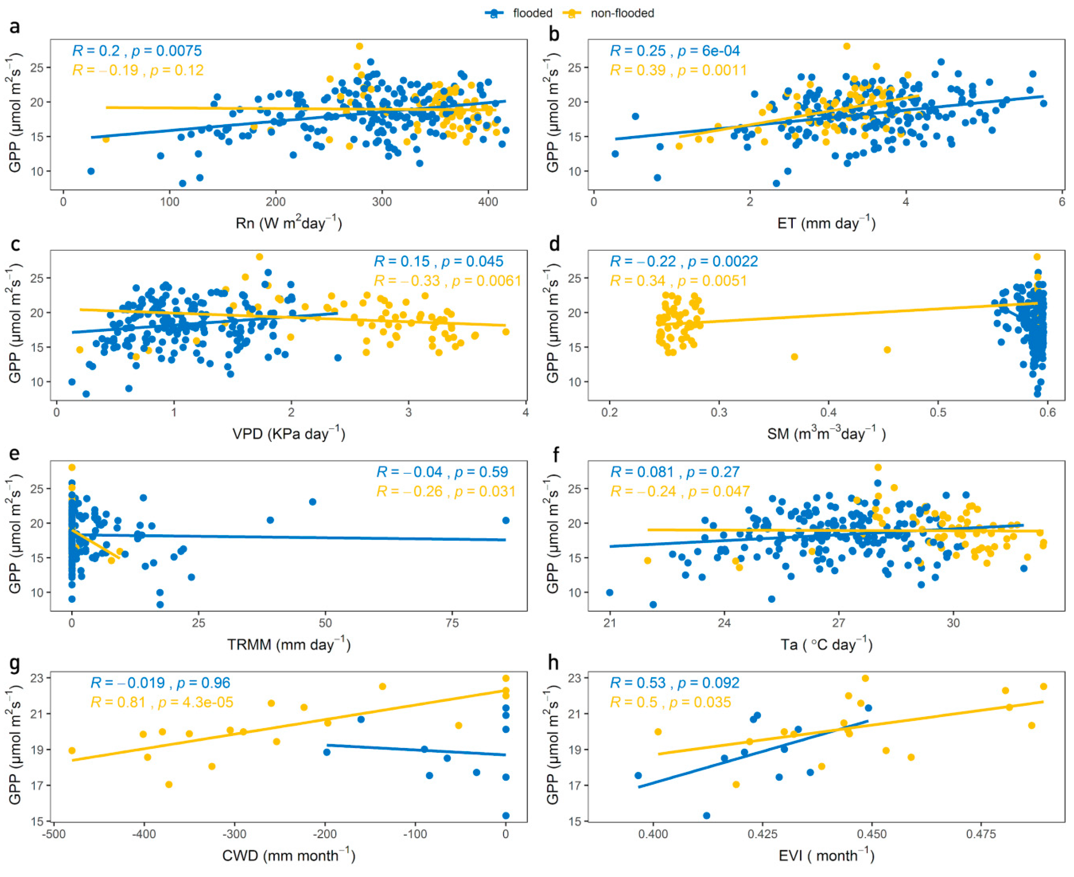
3.2. Correlation Between GPP, Climatic Variables and EVI

The relationship between GPP and Rn was positive during the flooded period (rho = 0.2, p < 0.05) and negative but not significant during non-flooded months (rho = −0.19, p = 0.12) (Figure 4a). GPP was positively associated with ET during both flooded (rho = 0.25, p < 0.05) and non-flooded months (rho = 0.38, p < 0.05) (Figure 4b).

Our analyses show that soil moisture and VPD are correlated with GPP in two contrasting ways. During the flooded period, soil moisture is negatively associated with GPP (rho = −0.22), while VPD is positively associated (rho = 0.15). However, during the non-flooded months, soil moisture is positively associated with GPP (rho = 0.34) and VPD negatively (rho = −0.33) (Figure 4c,d).

As GPP is in phase with soil moisture when the forest is not flooded, it decreases at the end of the dry season (September) and starts to increase in the onset of the rainy season (October). Nevertheless, a negative trend was observed between GPP and rainfall during non-flooded months (rho = −0.26, p < 0.05) (Figure 4e). Air temperature was negatively associated with GPP during non-flooded months (rho = −0.24, p < 0.05) and was not significant during the flooded months (rho = 0.081, p = 0.27) (Figure 4f).

Monthly CWD had the strongest positive association with GPP during non-flooded months (rho = 0.81, p < 0.05), to the extent that GPP increases when CWD gets less negative. No trend was observed during flooded months (rho = 0.01, p = 0.96) (Figure 4g).

As a proxy of photosynthetic capacity, EVI was positively correlated with GPP during non-flooded months (r = 0.50, p < 0.05) and despite not being significant, a positive trend was also observed during flooded months (r = 0.53, p = 0.09) (Figure 4h and Figure S6).

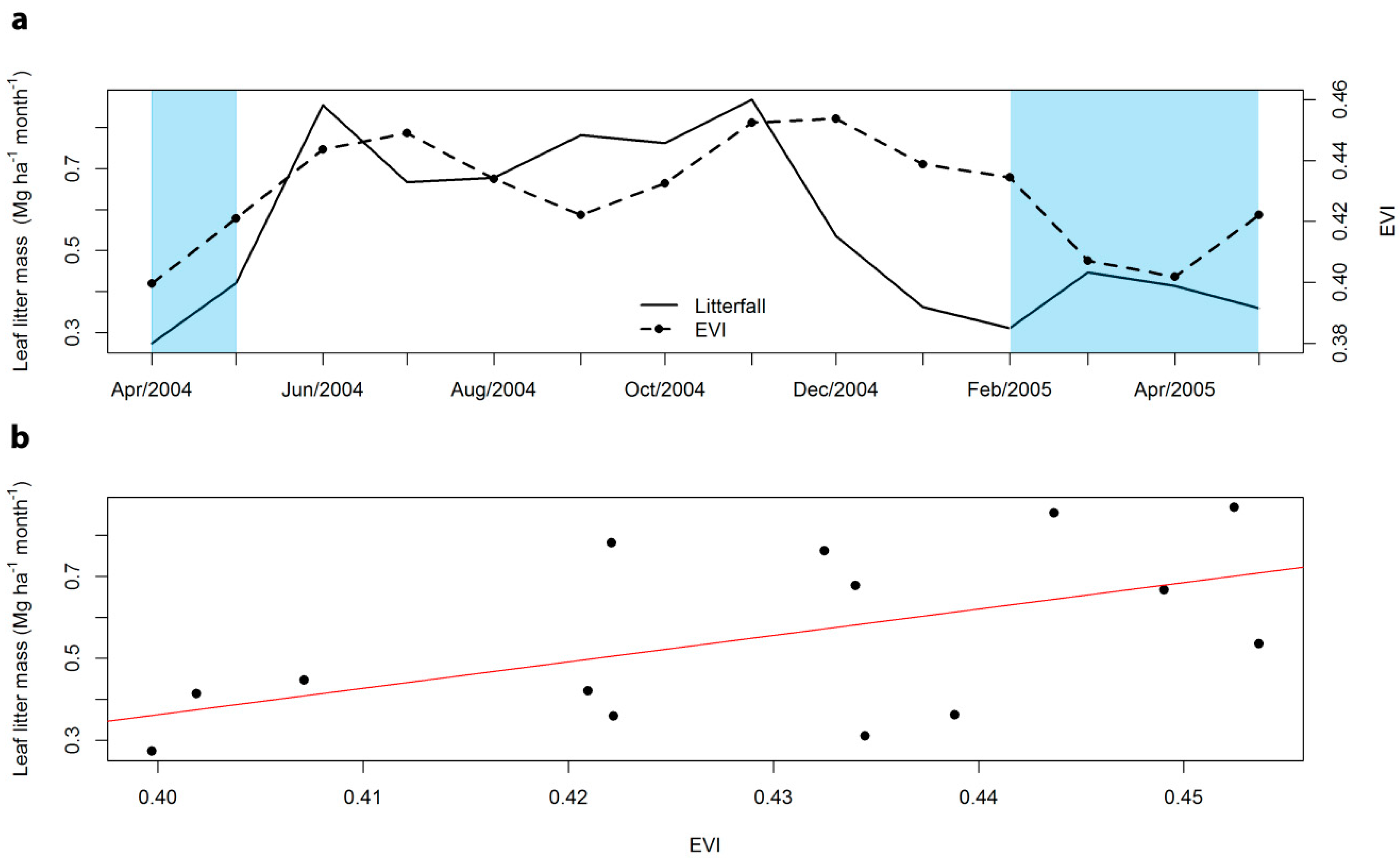
3.3. Seasonal Phenology Patterns and Analysis of Forest Canopy Gaps

Annual EVI was positively correlated to leaf litter mass (r = 0.55; p < 0.05). We observed one month lag between peaks in leaf litter mass (June and November) and EVI (July and December) (Figure 5). These observations suggest the months with greater leaf renewal would be June and November, which correspond to high peaks of seasonal GPP.

The canopy structure of our studied area had a mean height of 10.2 m (sd = 3.08), where most values from the canopy surface model are between the range of 4.8 and 14.9 m (5^th and 95^th percentile), and up to 38 m maximum height (Figure 6b). The canopy surface model shows the canopy is mostly closed with only 0.51% of the canopy area exhibiting gaps (height < 2 m), meaning that only a very small fraction of areas within the forest canopy would allow direct observation of the underlying understory. Although the LiDAR transect is 7 km away from the tower (Figure 6a), field measurements of tree height support our assumptions that the forest structure around the tower is similar to those of the LiDAR transect, as described in

Table 2. Experimental plots and LiDAR statistics regarding tree height measurements.

Plots	Number of Individuals	Tree Mean Height (m)	5% Percentile (m)	95% Percentile (m)	Maximum (m)
BAN1	86	11.79	6.84	18.86	28.36
BAN2	84	12.48	4.5	19.77	38.89
LiDAR	-	10.2	4.8	14.9	38

.

The EVI spatial correlation also showed that pixels within this transect are positively correlated to the tower EVI response through the time series analysis (r ≥ 0.6, p < 0.01). Hence, we argue there is no strong influence of free standing water on the EVI from MODIS-MAIAC observed during the flooded period, which could skew the observed phenological patterns.

3.4. Inter-Annual Variation of Seasonal Drivers and EVI-Multi-Angle Implementation Correction (MAIAC)

Our inter-annual EVI analysis showed that during extreme wet (2009) or dry (2016) years, phenology patterns have changed due to both excess and lack of water (Figure 7). During 2009, soil moisture was higher compared to other years (Figure 7e). Lower cumulative water deficit (Figure 7a) and lower temperatures (Figure 7b) was also recorded. On the other hand, during 2016, the river level was well below the mean, which decreased soil moisture (Figure 7e) in association with high temperatures and high VPD (Figure 7c). These changes on water availability have produced an anomalous EVI seasonal trajectory between these two years (Figure 7d).

The period of leaf exchange in 2009 occurred from July to December, while in 2016, there were two peaks of EVI, a small peak from April to June and another from October to November. Thus, we did not observe the bimodal pattern in 2009, and in 2016 leaf renewal and photosynthetic capacity period have changed due to the decrease of flooding and increases in atmospheric demands, observed through VPD, CWD and temperature.

4. Discussion

The annual average pattern of ET and GPP suggests that free water is exerting an influence on the evaporative processes during the flooded period since the peak of ET observed in March, matched the flooding peak. Our analysis confirms the free water evaporation hypothesis reported by Borma et al. [42] when observing higher values of ET during flood than during the dry season and lower GPP values [43].

This decoupled pattern of ET and GPP on the rainy-flooded period describes the forest dormancy probably due to anoxic conditions along the flooded months, as reported for Amazon flooded forests [34]. However, we observed the remaining high levels of GPP until March (one month after the flood started) and at the end of the flooded period (May), due to the shorter duration of the flooded period (or soil saturation) in higher terrain portions near the flux tower.

Conversely, both ET and GPP decrease during the dry period as a result of soil moisture depletion, with the lowest values of ET occurring at the end of the dry season (September), and the lowest values of GPP recorded in August/September. ET and GPP recover during the early rainy season (October to January), with the highest seasonal carbon assimilation rates from 20.40 to 22.63 μmol CO₂ m⁻² s⁻² [43]. The same growth and carbon assimilation pattern were reported in the central Amazonian floodplain, which exhibited greater productivity during the terrestrial phase, reaching on average 20 μmol CO₂ m⁻² s⁻² [32] and the highest growth rates from September to November [34]. At other Amazonian sites, GPP is maximized during the early dry season as a result of increasing incident radiation and reduction of cloudiness, coupled with high levels of ET [8,45], however, at the BAN site, GPP seasonality seems to be mainly governed by soil moisture which also regulates the canopy phenology.

The phenology pattern described by EVI suggests that the new leaves flush synchronized with senescence, which can be used as a proxy of canopy changes [11]. These peaks occur when GPP is maximized, suggesting the coupling between new leaves and phenology of photosynthetic capacity. Instead of light availability, EVI at this site seems to be strongly governed by soil moisture/aeration, differing from the terra firme forest [9]. However, over the flooded forests across the Amazon basin, a similar pattern is expected to occur as observed in this study, which is important for modeling carbon seasonality since approximately 14% of the basin is composed of flooded forests [28]. Nonetheless, phenology patterns obtained through satellite data in the central Amazon region should be interpreted carefully, since the flooding height is much higher than in this transitional area and assessments about the influence of flooding on vegetation indices should be considered. The EVI oscillation reflected the effect of soil moisture depletion at the end of the dry season, which reduced evapotranspiration and carbon assimilation rates, exhibiting the lowest peak in September. Thus, we highlight the potential of accurately monitoring of the floodplain forest phenology from spaceborne remote sensing, which described the carbon assimilation seasonality coupled with new leaves.

Previous studies have suggested two or more months of lag between canopy greening and forest productivity at terra firme forests [9,25], which could be explained by leaf demography [11]. Although our results have shown one month of decoupling between EVI and GPP during the dry season (May–Sep), at a flooded site, this lag could be an effect of topography within the tower footprint where the early GPP response is from sub-footprint regions that are topographically higher and drier. The EVI is characterizing the larger landscape response, where most forest area remains in likely anoxic conditions due to a longer period of inundation.

Our inter-annual analysis revealed a trend of increase in temperature and decrease of rainfall (Figure 7; Figure S7) as suggested by forecasts for this region [41,58], which is becoming drier over the last 10 years. The El Niño drought that significantly decreased rainfall and increased temperature in the Amazon basin during 2015/2016 [59] also affected this transition area, promoting a different vegetation response to environmental controls. The EVI suppression in 2009 reflected an extended dormant period due to soil saturation from January to June, while during these months in the ENSO year, EVI was slightly higher than the mean (Figure 7f), which was a result of the shorter flooded (eventually anoxic) period (Figure 7f). This seasonal EVI shift suggested that canopy changes are describing inter-annual water availability.

Hydroperiod has proven to be the main environmental control on above ground biomass in central Amazonian floodplains [60] and according to our findings, the hydrological regime also plays an important role in the seasonal vegetation response and consequently on the ecosystem productivity in our study region, at the southeast of the Amazon basin. These results suggest that changes in flooding patterns, which increases the duration and/or intensity of the dry season, could directly impact these areas, increasing tree mortality [39,61], wildfires [40] and CO₂ emissions [38], likewise reported for central Amazonian floodplain forests. Thus, it is important to analyze the seasonality of these flooded forests at landscape scales as we did in this study.

Although we found a significant relationship between GPP, leaf litter mass, and EVI computed from the moderate resolution images (MODIS), the forest seasonality approach could be investigated combining other remote sensing data with finer spatial resolution. In this context, the new products from the GEDI (Global Ecosystem Dynamics Investigation) and ECOSTRESS (ECOsystem Spaceborne Thermal Radiometer Experiment on Space Station) are an alternative to obtain Earth Observation data at a very high spatial and temporal resolution to investigate the carbon and water cycle in this forest.

5. Conclusions

Cycles of ecosystem productivity and evapotranspiration are decoupled in this southern Amazon flooded forest due to the dormancy period during flooded months, which influences the amount of free water evaporation and the decrease of productivity. The remaining high values of productivity at the beginning of the flooded period and before the flooding ends, in May, are explained by the shorter duration of soil saturation in higher terrain portions, concentrated near the flux tower. Although topographic differences in this floodplain forest only vary by 2 meters in height, some terrain portions are not subject to the same flood pulse, given the mean flood height of 1.3 m. Flooding also determines the amount of soil moisture during the non-flooded months, which is positively associated with productivity (rho = 0.34). To address the remote sensing challenges of detecting canopy phenology and productivity seasonality in this flooded area, we associated these ground measurements and leaf litter mass data with the EVI from MODIS-MAIAC and assessed the density of canopy gaps using airborne LiDAR data. Our results showed that EVI is positively associated with leaf litter mass (r = 0.55) and with GPP (r = 0.5), suggesting a coupling between new leaf production and phenology of photosynthetic capacity, with a bimodal productivity pattern of assimilating maximum carbon after the flooded period ends and during the rainy non-flooded season, under non-limiting soil water conditions. We also found that this forest has a very dense canopy, which means that free water exposed through gaps during the flooded period does not strongly influence EVI observations. Additionally, EVI described inter-annual variations of vegetation response to environmental drivers and revealed that water availability is the main phenological driver at this site, which can change vegetation phenology during extreme years, consequently affecting ecosystem productivity. Our study showed the potential for accurate monitoring of phenology in floodplain forests using spaceborne remote sensing.

References

1. Bonan, G.B. Forests and climate change: Forcings, feedbacks, and the climate benefits of forests. Science 2008, 320, 1444–1449. [Google Scholar] [CrossRef] [PubMed]
2. Pan, Y.; Birdsey, R.A.; Fang, J.; Houghton, R.; Kauppi, P.E.; Kurz, W.A.; Phillips, O.L.; Shvidenko, A.; Lewis, S.L.; Canadell, J.G.; et al. A large and persistent carbon sink in the world’s forests. Science 2011, 333, 988–993. [Google Scholar] [CrossRef] [PubMed]
3. Espírito-Santo, F.D.B.; Gloor, M.; Keller, M.; Malhi, Y.; Saatchi, S.; Nelson, B.; Junior, R.C.O.; Pereira, C.; Lloyd, J.; Frolking, S.; et al. Size and frequency of natural forest disturbances and the Amazon forest carbon balance. Nat. Commun. 2014, 5, 3434. [Google Scholar] [CrossRef] [PubMed] [Green Version]
4. Phillips, O.L.; Aragão, L.E.; Lewis, S.L.; Fisher, J.B.; Lloyd, J.; López-gonzález, G.; Malhi, Y.; Monteagudo, A.; Peacock, J.; Quesada, C.A.; et al. Drought sensitivity of the Amazon rainforest. Science 2009, 323, 1344–1348. [Google Scholar] [CrossRef] [PubMed]
5. Brienen, R.J.W.; Phillips, O.L.; Feldpausch, T.R.; Gloor, E.; Baker, T.R.; Lloyd, J.; Lopez-Gonzalez, G.; Monteagudo-Mendoza, A.; Malhi, Y.; Lewis, S.L.; et al. Long-term decline of the Amazon carbon sink. Nature 2015, 519, 344–348. [Google Scholar] [CrossRef] [PubMed] [Green Version]
6. Feldpausch, T.R.; Phillips, O.L.; Brienen, R.J.W.; Gloor, E.; Lloyd, J.; Malhi, Y.; Alarcón, A.; Dávila, E.Á.; Andrade, A.; Aragao, L.E.O.C.; et al. Amazon forest response to repeated droughts. Glob. Biogeochem. Cycles 2016, 30, 964–982. [Google Scholar] [CrossRef]
7. Gatti, L.V.; Gloor, M.; Miller, J.B.; Doughty, C.E.; Malhi, Y.; Domingues, L.G.; Basso, L.S.; Martinewski, A.; Correia, C.S.C.; Borges, V.F.; et al. Drought sensitivity of Amazonian carbon balance revealed by atmospheric measurements. Nature 2014, 506, 76–80. [Google Scholar] [CrossRef]
8. Restrepo-Coupe, N.; da Rocha, H.R.; Hutyra, L.R.; da Araujo, A.C.; Borma, L.S.; Christoffersen, B.; Cabral, O.M.R.; de Camargo, P.B.; Cardoso, F.L.; da Costa, A.C.L.; et al. What drives the seasonality of photosynthesis across the Amazon basin? A cross-site analysis of eddy flux tower measurements from the Brasil flux network. Agric. For. Meteorol. 2013, 182, 128–144. [Google Scholar] [CrossRef]
9. Wagner, F.H.; Hérault, B.; Rossi, V.; Hilker, T.; Maeda, E.E.; Sanchez, A.; Lyapustin, A.I.; Galvão, L.S.; Wang, Y.; Aragão, L.E.O.C. Climate drivers of the Amazon forest greening. PLoS ONE 2017, 12, e0180932. [Google Scholar] [CrossRef]
10. Chave, J.; Navarrete, D.; Almeida, S.; Álvarez, E.; Aragão, L.E.O.C.; Bonal, D.; Châtelet, P.; Silva-Espejo, J.E.; Goret, J.-Y.; von Hildebrand, P.; et al. Regional and seasonal patterns of litterfall in tropical South America. Biogeosciences 2010, 7, 43–55. [Google Scholar] [CrossRef] [Green Version]
11. Wu, J.; Albert, L.P.; Lopes, A.P.; Restrepo-Coupe, N.; Hayek, M.; Wiedemann, K.T.; Guan, K.; Stark, S.C.; Christoffersen, B.; Prohaska, N.; et al. Leaf development and demography explain photosynthetic seasonality in Amazon evergreen forests. Science 2016, 351, 972–976. [Google Scholar] [CrossRef] [PubMed] [Green Version]
12. Wu, J.; Kobayashi, H.; Stark, S.C.; Meng, R.; Guan, K.; Tran, N.N.; Gao, S.; Yang, W.; Restrepo-Coupe, N.; Miura, T.; et al. Biological processes dominate seasonality of remotely sensed canopy greenness in an Amazon evergreen forest. New Phytol. 2018, 217, 1507–1520. [Google Scholar] [CrossRef] [PubMed]
13. Huete, A.R.; Didan, K.; Shimabukuro, Y.E.; Ratana, P.; Saleska, S.R.; Hutyra, L.R.; Yang, W.; Nemani, R.R.; Myneni, R. Amazon rainforests green-up with sunlight in dry season. Geophys. Res. Lett. 2006, 33, 2–5. [Google Scholar] [CrossRef]
14. Saleska, S.R.; Didan, K.; Huete, A.R.; da Rocha, H.R. BREVIA Amazon Forests Green-Up During 2005 Drought. Science 2007, 318, 612. [Google Scholar] [CrossRef] [PubMed]
15. Anderson, L.O.; Malhi, Y.; Aragão, L.E.; Ladle, R.; Arai, E.; Barbier, N.; Phillips, O.; Anderson, L.O.; Ladle, R.; Arai, E.; et al. Remote sensing detection in Amazonian of droughts forest canopies. New Phytol. 2010, 187, 733–750. [Google Scholar] [CrossRef] [PubMed]
16. Brando, P.M.; Goetz, S.J.; Baccini, A.; Nepstad, D.C.; Beck, P.S.A.; Christman, M.C. Seasonal and interannual variability of climate and vegetation indices across the Amazon. Proc. Natl. Acad. Sci. USA 2010, 107, 14685–14690. [Google Scholar] [CrossRef] [PubMed] [Green Version]
17. Galvão, L.S.; dos Santos, J.R.; Roberts, D.A.; Breunig, F.M.; Toomey, M.; de Moura, Y.M. On intra-annual EVI variability in the dry season of tropical forest: A case study with MODIS and hyperspectral data. Remote Sens. Environ. 2011, 115, 2350–2359. [Google Scholar] [CrossRef]
18. Morton, D.C.; Rubio, J.; Cook, B.D.; Gastellu-Etchegorry, J.-P.; Longo, M.; Choi, H.; Hunter, M.O.; Keller, M. Amazon forest structure generates diurnal and seasonal variability in light utilization. Biogeosci. Discuss. 2016, 12, 19043–19072. [Google Scholar] [CrossRef]
19. Soudani, K.; François, C. Remote sensing: A green illusion. Nature 2014, 506, 165–166. [Google Scholar] [CrossRef] [PubMed]
20. Xu, L.; Samanta, A.; Costa, M.H.; Ganguly, S.; Nemani, R.R.; Myneni, R.B. Widespread decline in greenness of Amazonian vegetation due to the 2010 drought. Geophys. Res. Lett. 2011, 38, 2–5. [Google Scholar] [CrossRef]
21. Samanta, A.; Ganguly, S.; Myneni, R.B. MODIS enhanced vegetation index data do not show greening of amazon forests during the 2005 drought. New Phytol. 2011, 189, 11–15. [Google Scholar] [CrossRef] [PubMed]
22. Hilker, T.; Lyapustin, A.I.; Tucker, C.J.; Hall, F.G.; Myneni, R.B.; Wang, Y.; Bi, J.; Mendes de Moura, Y.; Sellers, P.J. Vegetation dynamics and rainfall sensitivity of the Amazon. Proc. Natl. Acad. Sci. USA 2014, 111, 16041–16046. [Google Scholar] [CrossRef] [PubMed] [Green Version]
23. Lyapustin, A.I.; Wang, Y.; Laszlo, I.; Hilker, T.; Hall, F.G.; Sellers, P.J.; Tucker, C.J.; Korkin, S.V. Multi-angle implementation of atmospheric correction for MODIS (MAIAC): 3. Atmospheric correction. Remote Sens. Environ. 2012, 127, 385–393. [Google Scholar] [CrossRef]
24. Lopes, A.; Walker, B.; Wu, J.; Maurício, P.; De Alencastro, L.; Valentim, J.; Prohaska, N.; Augusto, G.; Saleska, S.R. Remote Sensing of Environment Leaf fl ush drives dry season green-up of the Central Amazon. Remote Sens. Environ. 2016, 182, 90–98. [Google Scholar] [CrossRef]
25. Maeda, E.E.; Moura, Y.M.; Wagner, F.; Hilker, T.; Lyapustin, A.I.; Wang, Y.; Chave, J.; Mõttus, M.; Aragão, L.E.O.C.; Shimabukuro, Y. Consistency of vegetation index seasonality across the Amazon rainforest. Int. J. Appl. Earth Obs. Geoinf. 2016, 52, 42–53. [Google Scholar] [CrossRef]
26. de Moura, Y.M.; Hilker, T.; Lyapustin, A.I.; Galvão, L.S.; dos Santos, J.R.; Anderson, L.O.; de Sousa, C.H.R.; Arai, E. Seasonality and drought effects of Amazonian forests observed from multi-angle satellite data. Remote Sens. Environ. 2015, 171, 278–290. [Google Scholar] [CrossRef]
27. Maeda, E.E.; Ma, X.; Wagner, F.H.; Kim, H.; Oki, T.; Eamus, D.; Huete, A. Evapotranspiration seasonality across the Amazon Basin. Earth Syst. Dyn. 2017, 8, 439–454. [Google Scholar] [CrossRef] [Green Version]
28. Hess, L.L.; Melack, J.M.; Novo, E.M.L.M.; Barbosa, C.C.F.; Gastil, M. Dual-season mapping of wetland inundation and vegetation for the central Amazon basin. Remote Sens. Environ. 2003, 87, 404–428. [Google Scholar] [CrossRef]
29. Junk, W.J.; Piedade, M.T.F.; Wittmann, F.; Schöngart, J.; Parolin, P. Amazonian Floodplain Forests; 2011; Volume 53, ISBN 9788578110796. [Google Scholar]
30. De Simone, O.; Junk, W.J.; Schmidt, W. Central Amazon floodplain forests: Root adaptations to prolonged flooding. Russ. J. Plant Physiol. 2003, 50, 848–855. [Google Scholar] [CrossRef]
31. Parolin, P.; De Simone, O.; Haase, K.; Waldhoff, D. Central Amazonian floodplain forests: Tree adaptations in a pulsing system. Bot. Rev. 2004, 70, 357–380. [Google Scholar] [CrossRef]
32. Parolin, P.; Lucas, C.; Piedade, M.T.F.; Wittmann, F. Drought responses of flood-tolerant trees in Amazonian floodplains. Ann. Bot. 2010, 105, 129–139. [Google Scholar] [CrossRef] [PubMed]
33. Finlayson, M.; Lévêque, C.; Randy Milton, G.; Peterson, G.; Pritchard, D.; Ratner, B.D.; Reid, W.V.; Revenga, C.; Rivera, M.; Schutyser, F.; et al. A Report of the Millennium Ecosystem Assessment. Available online: https://www.millenniumassessment.org/documents/document.356.aspx.pdf. (accessed on 20 February 2019).
34. Schongart, J.; Piedade, M.T.F.; Horna, V.; Worbes, M. Phenology and stem-growth periodicity of tree species in Amazonian floodplain forests. J. Trop. Ecol. 2002, 18, 581–597. [Google Scholar] [CrossRef] [Green Version]
35. Schongart, J.; Junk, W.J.; Piedade, M.T.F.; Ayres, J.M.; Hüttermann, A.; Worbes, M. Teleconnection between tree growth in the Amazonian floodplains and the El Niño—Southern Oscillation effect. Glob. Chang. Biol. 2004, 10, 683–692. [Google Scholar] [CrossRef]
36. Teresa Fernandez Piedade, M.; Junk, W.J.; Parolin, P. The flood pulse and photosynthetic response of trees in a white water floodplain (várzea) of the Central Amazon, Brazil. SIL Proc. 1922–2010 2000, 27, 1734–1739. [Google Scholar] [CrossRef]
37. Nobre, C.A.; Sampaio, G.; Borma, L.S.; Castilla-Rubio, J.C.; Silva, J.S.; Cardoso, M. Land-use and climate change risks in the Amazon and the need of a novel sustainable development paradigm. Proc. Natl. Acad. Sci. USA 2016, 113, 10759–10768. [Google Scholar] [CrossRef] [PubMed] [Green Version]
38. Dalmagro, H.J.; Zanella de Arruda, P.H.; Vourlitis, G.L.; Lathuillière, M.J.; de S. Nogueira, J.; Couto, E.G.; Johnson, M.S. Radiative forcing of methane fluxes offsets net carbon dioxide uptake for a tropical flooded forest. Glob. Chang. Biol. 2019, 4, 1967–1981. [Google Scholar] [CrossRef] [PubMed]
39. de Resende, A.F.; Schöngart, J.; Streher, A.S.; Ferreira-Ferreira, J.; Piedade, M.T.F.; Silva, T.S.F. Massive tree mortality from flood pulse disturbances in Amazonian floodplain forests: The collateral effects of hydropower production. Sci. Total Environ. 2019, 659, 587–598. [Google Scholar] [CrossRef] [PubMed]
40. Scheffer, M.; Mesquita, R.C.G.; Flores, B.M.; Holmgren, M.; Jakovac, C.C.; Xu, C.; van Nes, E.H. Floodplains as an Achilles’ heel of Amazonian forest resilience. Proc. Natl. Acad. Sci. USA 2017, 114, 4442–4446. [Google Scholar]
41. Malhi, Y.; Wright, J. Spatial patterns and recent trends in the climate of tropical rainforest regions. Philos. Trans. R. Soc. B Biol. Sci. 2004, 359, 311–329. [Google Scholar] [CrossRef]
42. Borma, L.S.; Da Rocha, H.R.; Cabral, O.M.; Von Randow, C.; Collicchio, E.; Kurzatkowski, D.; Brugger, P.J.; Freitas, H.; Tannus, R.; Oliveira, L.; et al. Atmosphere and hydrological controls of the evapotranspiration over a floodplain forest in the Bananal Island region, Amazonia. J. Geophys. Res. Biogeosci. 2009, 114, G01003. [Google Scholar] [CrossRef]
43. Costa, G.P. Fluxos de energia, CO2 e CH4 Sobre a Floresta em Planície de Inundação da Ilha do Bananal. Ph.D. Dissertation, Federal University of São Paulo, São Paulo, Brazil, 2015. Available online: http://www.teses.usp.br/teses/disponiveis/91/91131/tde-28092015-111609/ (accessed on 15 October 2018).
44. Homeier, J.; Kurzatkowski, D.; Leuschner, C. Stand dynamics of the drought-affected floodplain forests of Araguaia River, Brazilian Amazon. For. Ecosyst. 2017, 4, 10. [Google Scholar] [CrossRef]
45. Da Rocha, H.R.; Manzi, A.O.; Cabral, O.M.; Miller, S.D.; Goulden, M.L.; Saleska, S.R.; Coupe, N.R.; Wofsy, S.C.; Borma, L.S.; Artaxo, R.; et al. Patterns of water and heat flux across a biome gradient from tropical forest to savanna in brazil. J. Geophys. Res. Biogeosci. 2009, 114, 1–8. [Google Scholar] [CrossRef]
46. Hayek, N.H.; Longo, M.; Wu, J.; Smith, M.N.; Restrepo-coupe, N.; Tapajós, R.; Da Silva, R.; Fitzjarrald, D.R.; Camargo, P.B.; Hutyra, L.R.; et al. Carbon exchange in an Amazon forest: From hours to years. Biogeosciences 2018, 15, 4833–4848. [Google Scholar] [CrossRef]
47. Cabral, O.M.R.; Gash, J.H.C.; Rocha, H.R.; Marsden, C.; Ligo, M.A.V.; Freitas, H.C.; Tatsch, J.D.; Gomes, E. Fluxes of CO2 above a plantation of Eucalyptus in southeast Brazil. Agric. For. Meteorol. 2011, 151, 49–59. [Google Scholar] [CrossRef]
48. Hutyra, L.R.; Munger, J.W.; Saleska, S.R.; Gottlieb, E.; Daube, B.C.; Dunn, A.L.; Amaral, D.F.; de Camargo, P.B.; Wofsy, S.C. Seasonal controls on the exchange of carbon and water in an Amazonian rain forest. J. Geophys. Res. Biogeosci. 2007, 112. [Google Scholar] [CrossRef]
49. Moreira, K.S.; Rocha, H.R.; Kurzatkowski, D.; Ribeiro da Mata, R.; Pinto, A.S. Avaliação na Queda de Liteira em Ecótonos no Entorno da Ilha do Bananal. In Proceedings of the 2nd Congress of Students and Scholars of the LBA Experiment, Manaus, Brazil, 1–13 July 2005; Available online: http://lba2.inpa.gov.br/lbaconferencias/2005_lba_student_conf/index.htm (accessed on 12 February 2019).
50. Dalagnol, R.; Wagner, F.H.; Galvão, L.S.; Nelson, B.W.; Oliveira, E. Life cycle of bamboo in southwestern Amazon and its relation to fire events. Biogeosciences 2018, 15, 6087–6104. [Google Scholar] [CrossRef]
51. Dalagnol, R.; Wagner, F.H.; Galvão, L.S.; Aragão, L.E.O.eC. The MANVI Product: MODIS (MAIAC) Nadir-Solar Adjusted Vegetation Indices (EVI and NDVI) for South America, Version v1; Zenodo, 2019. Available online: https://0-doi-org.brum.beds.ac.uk/10.5281/zenodo.3159488 (accessed on 25 June 2019).
52. Huete, A.; Didan, K.; Miura, T.; Rodriguez, E.; Gao, X.; Ferreira, L. Overview of the radiometric and biophysical performance of the MODIS vegetation indices. Remote Sens. Environ. 2002, 83, 195–213. [Google Scholar] [CrossRef]
53. Hansen, M.C.; Potapov, P.V.; Moore, R.; Hancher, M.; Turubanova, S.A.; Tyukavina, A.; Thau, D.; Stehman, S.V.; Goetz, S.J.; Loveland, T.R.; et al. High-Resolution Global Maps of 21st-Century Forest Cover Change. Science 2013, 850, 2011–2014. [Google Scholar] [CrossRef]
54. Dee, D.P.; Uppala, S.M.; Simmons, A.J.; Berrisford, P.; Poli, P.; Kobayashi, S.; Andrae, U.; Balmaseda, M.A.; Balsamo, G.; Bauer, P.; et al. The ERA-Interim reanalysis: Configuration and performance of the data assimilation system. Q. J. R. Meteorol. Soc. 2011, 137, 553–597. [Google Scholar] [CrossRef]
55. Aragão; Luiz Eduardo, O.C.; Malhi, Y.; Roman-Cuesta, R.M.; Saatchi, S.; Anderson, L.O.; Shimabukuro, Y.E. Spatial patterns and fire response of recent Amazonian droughts. Geophys. Res. Lett. 2007, 34, 1–5. [Google Scholar] [CrossRef]
56. Hunter, M.O.; Keller, M.; Morton, D.; Cook, B.; Lefsky, M.; Ducey, M.; Saleska, S.; De Oliveira, R.C.; Schietti, J.; Zang, R. Structural dynamics of tropical moist forest gaps. PLoS ONE 2015, 10, 1–19. [Google Scholar] [CrossRef] [PubMed]
57. Tavares, I.B.; Borma, L.S.; Fonseca, L.D.M.; Collicchio, E.; Domingues, T.F.; Rocha, H.R. The growth pattern of the forest located in a southeast Amazonian floodplain during the 2015/2016 ENSO year. Ecohydrology 2019. under review. [Google Scholar]
58. Gloor, M.; Barichivich, J.; Ziv, G.; Brienen, R.; Schöngart, J.; Peylin, P. Recent Amazon climate as background for possible ongoing Special Section. Glob. Biogeochem. Cycles 2015, 29, 1384–1399. [Google Scholar] [CrossRef]
59. Jiménez-Muñoz, J.C.; Mattar, C.; Barichivich, J.; Santamaría-Artigas, A.; Takahashi, K.; Malhi, Y.; Sobrino, J.A.; Schrier, G. Van Der Record-breaking warming and extreme drought in the Amazon rainforest during the course of El Niño 2015–2016. Sci. Rep. 2016, 6, 33130. [Google Scholar] [CrossRef] [PubMed]
60. Schöngart, J.; Haugaasen, T.; Wittmann, F.; Piedade, M.T.F.; Bredin, Y.K.; de Assis, R.L.; Nobre Quesada, C.A. Above-ground woody biomass distribution in Amazonian floodplain forests: Effects of hydroperiod and substrate properties. For. Ecol. Manag. 2018, 432, 365–375. [Google Scholar]
61. Piedade, M.T.F.; Schöngart, J.; Wittmann, F.; Parolin, P.; Junk, W.J. Impactos ecológicos da inundação e seca na vegetação de áreas alagáveis amazônicas. In Eventos Climáticos Extremos na Amazônia Causas e Conseqüências; Oficina de Textos: São Paulo, Brazil, 2013; pp. 268–304. [Google Scholar]
Figure 1. Large-scale biosphere-atmosphere (LBA) eddy flux tower location. (A) Tocantins State inside Legal Amazon delimitation (red line), (B) Cantão State Park location in the transition area between the Amazon and Cerrado biomes (Brazilian Institute of Geographic Statistics (IBGE) delimitation, green and beige), and (C) LBA tower inside Cantão State Park (Sentinel-2 image, red-green-blue (RGB) composite of June 2018).
Remotesensing 11 01530 g001
Figure 2. Average annual cycle of ET (2004 to 2014; black line) and rainfall from TRMM (2004 to 2016; dark grey bar) (a), cumulative water deficit (2004 to 2016; CWD) (b), vapour pressure deficit (2004 to 2014; VPD) (c), soil moisture (2004 to 2016; SM) and flood height (2004 to 2016; dark blue line) (d), net radiation (2004 to 2016; dashed black line) and air temperature (2004 to 2014; brown solid line) (e), GPP (2011 to 2013; black solid line) (f), and EVI (2004 to 2016; long dashed black line) (g). The shaded blue area corresponds to the flooded period.
Remotesensing 11 01530 g002
Figure 3. Shuttle Radar Topographic Mission (SRTM) classified as areas below and above the tower level, which is located at 181 meters of altitude (red dot). Grey squares represent the Moderate Resolution Imaging Spectroradiometer (MODIS) pixels within the tower footprint (green circle, Borma et al. [42]) selected to extract mean EVI and be analyzed.
Remotesensing 11 01530 g003
Figure 4. Scatterplots between the daily mean of eddy covariance GPP compared to climate drivers from2011 to 2013: Net radiation (a), ET (b), VPD (c), Average soil moisture for layers up to 200 cm depth (d), Rainfall (e), Ta (f) and the monthly average of GPP compared to CWD (g) and EVI (h). Both lines represent the regression fit between variables during flooded (blue) and non-flooded (yellow) months.
Remotesensing 11 01530 g004
Figure 5. Monthly average leaf litter mass rate (solid black line) collected at the surrounding area of the tower from April 2004 to May 2005 [49], and monthly average EVI-multi-angle implementation correction (MAIAC) (black dashed line) for the same period. The flooded period is represented by the blue shading area (a). Scatterplot between EVI and leaf litter mass with the fitted regression line (red) (b).
Remotesensing 11 01530 g005
Figure 6. (a) Spatial and temporal correlation between tower EVI and pixels with less than 10% of permanent water channels [52] inside the Cantão State Park. (b) LiDAR canopy height model (CHM) transect and gaps (< 2m height) in red.
Remotesensing 11 01530 g006
Figure 7. Monthly variation of CWD (a), temperature (b), VPD (c), river level (d), soil moisture (e) and EVI (f). The dashed line represents the average value (2004–2016), the standard deviation of the monthly variables is indicated by the grey shading, the blue line represents the wettest year (2009), the red line the driest year (2016) and grey lines represent remaining years (2004–2015).
Remotesensing 11 01530 g007