Investigating the Consistency of Uncalibrated Multispectral Lidar Vegetation Indices at Different Altitudes


1
Department of Geography, University of Lethbridge, Lethbridge, AB T1K 3M4, Canada
2
Institute of Mathematical Problems of Biology RAS, branch of the M.V.Keldysh Institute of Applied Mathematics of the Russian Academy of Sciences, 1 Prof. Vitkevich St, Pushchino, Moscow Region 142290, Russia
*
Author to whom correspondence should be addressed.
Remote Sens. 2019, 11(13), 1531; https://0-doi-org.brum.beds.ac.uk/10.3390/rs11131531
Submission received: 22 May 2019
/
Revised: 15 June 2019
/
Accepted: 19 June 2019
/
Published: 28 June 2019
(This article belongs to the Special Issue Future Trends and Applications for Airborne Laser Scanning)
Abstract
:Multi-spectral (ms) airborne light detection and ranging (lidar) data are increasingly used for mapping purposes. Geometric data are enriched by intensity digital numbers (DNs) and, by utilizing this additional information either directly, or in the form of active spectral vegetation indices (SVIs), enhancements in land cover classification and change monitoring are possible. In the case of SVIs, the indices should be calculated from reflectance values derived from intensity DNs after rigorous calibration. In practice, such calibration is often not possible, and SVIs calculated from intensity DNs are used. However, the consistency of such active ms lidar products is poorly understood. In this study, the authors reported on an ms lidar mission at three different altitudes above ground to investigate SVI consistency. The stability of two families of indices—spectral ratios and normalized differences—was compared. The need for atmospheric correction in case of considerable range difference was established. It was demonstrated that by selecting single returns (provided sufficient point density), it was possible to derive stable SVI products. Finally, a criterion was proposed for comparing different lidar acquisitions over vegetated areas.
1. Introduction
Light detection and ranging (lidar) established itself as a unique high-resolution remote sensing technology due to its 3D sampling of land cover and terrain, and its ability to penetrate and characterize vegetation structures from treetop to ground [1]. Lidar is primarily used to construct detailed digital elevation models (DEMs), but the intensity channel (an index of received signal power) is increasingly used in a similar fashion to black and white aerial photographs or single channels in multispectral imagery. Using passive imagery, numerous spectral vegetation indices (SVIs) have been developed based on reflectance values derived from image-based DNs for environmental monitoring and change detection [2,3,4]. Modern multi-spectral lidar technology allows for active narrow-band vertical spectral sampling of vegetation profiles and provides an alternative method of deriving SVI maps, active SVIs, which present a new tool for high resolution thematic mapping, enhanced classification and change detection, and forest resource monitoring [5].
In general, the main limitation of spectral vegetation indices derived from passive remote sensing imagery is the dependence on the sun as a source of illumination [6], which leads to sensitivity of passive SVIs to sun position [7] and cloudiness [8]. In addition, passive SVIs as quantitative indicators of vegetation phenology characteristics are affected by canopy structural properties, background scene, and leaf surface, shape, and orientation [9]. The benefit of lidar, as an active sensor that measures the backscatter signal, is its ability to collect data without an external source of illumination and its potential to eliminate multiple scattering and geometric viewing effects [10,11]. Additionally, for a small-footprint system, background radiance can be easily separated from the canopy response. The main factors affecting lidar backscatter, besides the spectral reflectance properties of the target, are the area of effective backscattering surface and the local incidence angle of the target [10]. However, if the optical path at different wavelength channels is similar, like in the sensors described by Hakala et al. [12] and Morsdorf et al. [11], or close to each other, like in the Titan ms lidar, it can be assumed that the influence of these factors is reduced or potentially canceled in active SVIs. Consequently, to maximize the utility and comparability of active SVIs, it is necessary to study their consistency through different sensors and/or different survey configurations.
1.1. The Titan Spectral Vegetation Indices
In general, if there are a number of spectral bands of some particular sensor, one can construct, following Rees [13], two types of indices—the simple ratio index (sρ) and the normalized difference index (nδ) by the following mathematical expressions:
Here, and denote spectral reflectance of the target (or scene) at the lth and mth channel/band. There is an obvious non-linear relation between these two indices [14]:
The first SVIs were introduced as a result of an effort to reduce multispectral measurements of Landsat I to a single value [14,15] and inevitably referred to the available Landsat spectral bands. Following the same logic, our interest in SVIs can be limited to the wavelengths of 532 nm, 1064 nm, and 1550 nm, which are used for the Teledyne Optech Titan sensor channels C3, C2, and C1—a brief description of the system can be found in [16]. Thus, six sρ indices and correspondingly, six nδ indices can be constructed. However, due to symmetry:
only three spectral ratio indices and three normalized difference indices will be considered further which will be referred to as sρ(Cl,Cm) and nδ(Cl,Cm) with l, m indices corresponding to the Titan’s channel numbers or, for indicating the actual wavelengths, as and .
In passive imagery, the abbreviation NDVI (normalized difference vegetation index) is typically reserved for the combination of red and near-infrared (NIR) bands [4]. This index helps to distinguish vegetated areas on an image due to the way light reflects from vegetation. Spectral signatures of green vegetation are well known [17]. Spectral reflectance is low in the visible range, with a peak in the green region. This is due to absorption of light by chlorophyll and other pigments in leaf tissue. The following sharp increase in the spectral reflectance curve is referred to as the red edge. After the red edge, there is a region of relatively high reflectance known as the NIR plateau. The leaf cell structure dominates the response in this region. After the NIR plateau, there are two regions of lower reflectance at approximately 1450 nm and 1950 nm due to absorption by water in the leaf tissue, with a region of increased reflectance in-between.
From the vegetation spectral reflectance curve [13], it is possible to distinguish vegetated and non-vegetated areas by adopting a broader definition of NDVI, as the normalized difference in reflectance between NIR and any of the visible bands. For example, the Advanced Very High Resolution Radiometer (NOAA AVHRR) sensor has only one band for the visible spectrum. Using this approach, Titan’s index is comparable to a commonly defined and utilized NDVI. Moreover, in narrow-band hyperspectral passive imagery, another index referred as photochemical reflectance index (PRI) was developed for assessing the canopy photosynthetic light use efficiency of vegetation [18]. This index is based on a change in canopy reflectance at 531 nm with interconversion of the xanthophyll cycle pigments, a process which is closely linked to light absorption. Currently, the most commonly used definition of PRI is the normalized difference between the 531 nm and the 570 nm wavebands, with the latter being used as a reference. However, in the original work [19] Gamon et al. introduced PRI using our notation, and, assuming that reflectance of the canopy at 1064 nm does not change with overexposure to light, Titan’s nδ(C2, C3) properties may be comparable to PRI.
For passive imagery, it has been shown that the normalized difference infrared index (NDII), which utilized near-infrared (0.7–1.3 µm) and middle-infrared (MIR, 1.3–2.5 µm) wavelengths, is highly correlated with canopy water content [20] and was applied for the detection of plant water stress [21]. In a recent study, Hancock et al. [22], investigated angular reflectance of leaves with a dual-wavelength terrestrial lidar system and its implications for leaf-bark separation and leaf moisture estimation, and showed that change in the normalized difference index (NDI, at 1063 nm and 1545 nm) associated with leaf water content was larger than the change related to the angle of incidence. In our notation, this index is close to Titan’s . In addition, Chasmer et al. [23] proposed an active normalized burn ratio (ANBR) derived from the ms lidar 1064 nm and 1550 nm channels as an index of burn severity in vegetated areas, which they compared to the passive normalized burn ratio derived from Landsat data.
Finally, the normalized difference of the green band and MIR was used by Xu [24] for distinguishing water bodies from the soil, vegetation, and man-made features. In a recent study, Morsy et al. [25] suggested using Titan’s NDVINIR-G () for vegetation extraction. It is yet to be found what this index represents in the canopy.
1.2. Lidar Radiometry
Radiometry characterizes or measures how much electromagnetic energy is associated with some location or direction in space [26]. In case of lidar this is the target’s intensity response to the emitted laser pulse. The relationship between transmitted and received laser pulse power in the far field is given by the radar equation in the form of [27]:
where: Pr is received signal power, Pt —transmitted power, D—aperture diameter, R—system range to target, μatm—atmospheric transmission factor, μsys—system transmission factor, θt—transmitter beam width, and σ—effective target cross section.
The effective target cross section is defined as [27]:
where Ω is scattering steradian solid angle of target, ∂A—target area, and target reflectivity. It should be noted that in current literature (for instance [28]), target reflectivity from [27] is often defined as the biconical reflectance , a function dependent on scattered cone and the incident flux cone (see Section 1.4 for an extended explanation). However, assuming a standard scattering diffuse target (Lambertian target) with reflectance , Equation (7) can be re-written:
The area Afp, illuminated by a circular beam at a range R at nadir, is:
Note that beam divergence θt is provided for only part of the spatial energy beam profile (e.g., Gaussian at 1/e or 1/e2), therefore, Afp only approximates the total illuminated area. If a target intercepts the entire beam, it is referred to as an extended target. If the target area is smaller than the transmitted footprint, it is referred to as a point target. Thus, for an extended Lambertian target substituting ∂A with Afp [27]:
leads to the radar equation in the form [27]:
For a point Lambertian target, the radar equation can be re-written in the form:
1.3. Lidar Intensity Metrics
The intensity of small-footprint systems has been shown to be useful in land cover classification [31], tree species classification [32], fractional cover estimation [33], and carbon estimates in forest biomass [34]. Although many studies have shown the utility of all returns [33,35], some studies use the intensity of the first returns [32,36]. Korpela et al. [37] explained that the choice of working with first returns was made because of insufficient point density of single returns in the study dataset. Usually, intensity metrics are calculated by averaging values in raster grids of a certain size, after range normalization, or, if possible, after rigorous calibration [38]. The procedure of rasterization with an assigned average value can be written for grids of only extended Lambertian targets, with an index i running through points inside a given cell:
Here the notation <xi> is used to denote rasterization of an attribute x associated with a point from the lidar point cloud by averaging (< >) through i numbers of attribute values from corresponding i points inside a grid cell. It is assumed that intensity DN (I) is a linear function of the received peak power (I = kPr) and range normalization to the range ℝ was applied to intensity DNs. Then, assuming that atmospheric losses, transmission power, and the system transmission factor are constant, the above equation can be re-written in the form of (denoting intensity normalized to inverse square range as ):
It should be noted that the above simplification due to the assumption of constant atmospheric losses, transmission power, and the system transmission factor should be a subject of verification to estimate introduced bias. For instance, in the case of atmospheric losses, Equation (14) disregards difference due to different ranges at slant angles and adjacent flight lines. In the case of the transmission power stability and the system transmission factor, it is well known, that manufacturers put special effort to achieve such characteristics of the sensor, but these factors should be controlled if possible. The same procedure can be performed for point Lambertian targets, and using the same assumptions, the corresponding equation can be written as:
Or, if we use area Afp from Equation (9) as a normalization value:
Interpretation of a single return intensity from an extended target is quite straightforward, as it represents an average reflectance over the grid. However, in the case of single returns from vegetation, this is generally not true. For a lidar beam, vegetation represents a porous 3D target leading to a lengthening (in time) of the response return and, in effect, causes volumetric backscattering. The process can be described in mathematical terms as a convolution of the emitted pulse with a differential effective cross-section of each cluster of inseparable targets [39]. Thus, the peak of the intensity does not quantitatively correspond to the energy scattered by the particular volume of the target with the same coefficient as in the case of a flat extended target. However, assuming a Gaussian distribution along the beam propagation, such returns in full waveform (FWF) systems can be calibrated by utilizing the pulse width information from the returned signal waveform [40]. In case of DR systems, this information is not available and one can only assume similarity of volumetric return widths. Moreover, in case of FWF scanners, a response signal of the system to an emitted pulse is recorded, and it was shown [40] that this waveform is also a convolution (in time) of the received signal with the detector response function. The latter should be used for more accurate analysis of the lidar intensity DNs. Interpretation of the multiple return intensity in rasterized products is more complex. As can be seen from Equation (16), it is a mix of geometric and radiometric information.
1.4. Angular Effects of Lidar Backscatter
In Equation (7), explicit consideration of the angle between the surface of the target and the lidar beam was omitted, and lumped into reflectance ρ by assuming the target was an ideal diffuse Lambertian reflector. This is a common approach in the interpretation of lidar backscatter, and a backscatter coefficient [28,39] is used to combine the Lambertian assumption with normalization of the lidar backscatter to the illuminated area. However, in general, the reflectance of a particular object is more complex and described by a corresponding bidirectional reflectance distribution function (BRDF) [41]. The ideal Lambertian diffuse target assumption simplifies analytical solutions in passive imagery but, in lidar radiometry, it leads to a well-known cosine correction [40]. Alternatively, an ideal isotropic diffuse target assumption allows the omission of a cosine correction and simplifies analytical formulas for active imagery. While both models represent simplifications of an actual BRDF, work by Kukko et al. [42] suggested that ideal isotropic diffuse reflectance might be a better assumption for certain materials. For vegetation, the work of Govaerts et al. [43] demonstrated that neither of the simple diffuse models was correct. Alternatively, a concept of apparent reflectance was developed by Li et al [44] for calibrating dual-wavelength terrestrial lidar resulting in improved quantification of vegetation structure and allowing for better comparison of lidar datasets from different instruments and campaigns. At the same time, the research on angular effects of lidar backscatter in vegetation is sparse and among the recent literature, the work of Hancock et al. [22] can be highlighted in which the authors investigated leaf moisture estimation and leaf-bark separation.
1.5. Relevant Studies and Impetus for the Experiment
As mentioned above, SVIs are widely used and of immediate practical interest in many applications. However, a challenge in the case of ms lidar is that true surface reflectance is not equivalent to pulse return signal intensity DN. Reflectance is a spectral characteristic of the target, while the intensity captured by commercial lidar sensors is an index of peak signal backscatter amplitude, which is further influenced by sensor and data acquisition characteristics [30]. Without calibration targets [40,45] or a proven model which accounts for the system and external factors (e.g., atmospheric conditions), it is not possible to accurately calculate reflectance from intensity DN. Using calibration targets often is not practical, and, currently, most of the characteristics of a particular system are considered a manufacturer’s intellectual property and are not readily provided for precise modeling. It is possible, however, to conduct an independent calibration of a given system for a particular application [46,47]. Consequently, the adoption of SVIs calculated from ms lidar intensity DNs can be foreseen, leading to questions of how consistent such products might be given the potential range of conditions under which the DNs could be collected. Moreover, from Equation (16), it can be seen that in the case of split (multiple) returns, average intensity is not a wholly spectral characteristic, and this raises the question of how SVIs calculated with this metric might differ from SVIs derived from single return intensities over the same vegetated area.
In [5], Titan intensity responses were compared with values obtained from three single-wavelength (corresponding to Titan’s) sensors and noted that the intensity distributions obtained from the Titan were closer to each other due to the Titan system design considerations. As radiometric targets were not used for the study above, it is not possible to compare SVIs derived from single-wavelength sensors to those of Titan. However, if the same ms lidar system is flown over the same area at different altitudes during the same time window, it is possible to compare the consistency of ratio-based SVIs derived from the different channels of lidar emission wavelengths for different altitudes. Therefore, an experimental survey was conducted with the Titan sensor at three different altitudes above ground: 500 m, 1000 m, and 1500 m (note that 1500 m is higher than 1070 m from [5]).
1.6. Hypothesis and Objectives
1.6.1. Single Channel Intensity Ratios
It is expected that, for extended targets, intensity normalized to inverse square range single-channel ratios follow the radiometric equation (we denoted height above ground as H1 < H2 < H3):
For example, increases in ratio (Equation (17)) are expected to be seen due to atmospheric transmission losses. However, for vegetated areas it is unclear how single-channel ratios of averaged intensity from all returns, and from single returns, compare to the extended target return ratios. The underlying assumption is that the emitted signal power output is stable; i.e., the observed single channel intensity (normalized to inverse square range) ratios should differ more for flight lines from different altitudes than those collected from the same altitude. Work by Okhrimenko and Hopkinson [47] reported only 2% difference in derived reflectance means over calibrated targets from different flight lines at approximately the same flight altitude, with a maximum observed deviation of 6% for C1 (1550 nm) channel, and 4% for C2 (1064 nm) and C3 (532 nm) channels for the same Teledyne Optech Titan sensor. Atmospheric losses, on the other hand, can be estimated within 10–50% by the Bourges-Lambert law with an extinction coefficient (dependent on spectral and atmospheric conditions) of approximately 0.1–0.2 km−1 [27] for an increased range of 500 m–1000 m.
1.6.2. Comparison of Point Density Distributions across Three Altitudes
It is understood that with increasing survey altitude, the density of points over vegetated areas will decrease, both due to sampling geometry and pulse energy extinction, eventually reaching zero. In Hopkinson et al. [5] it was reported that the average intensity value (a unit-less index) at a flight altitude of 1070 m AGL (above ground level) was low (12.4) for C3 (532 nm). Thus, for the purpose of extracting SVIs from ms lidar data, it is crucial to adopt survey parameters (e.g., AGL) that enable sufficient point density for analysis. Moreover, because of the complex interpretation of rasterized multiple return intensity products, there is value in rasterized single return products, as their radiometric meaning and interpretation is simpler.
1.6.3. Consistency of Spectral Vegetation Indices through Different Altitudes
Here, the consistency and behavior of active laser SVIs sampled from different altitudes is evaluated. The expectation is that spectral indices are consistent over extended targets. However, over vegetated areas consistency is likely to be influenced by sample point density, differential canopy attenuation with each channel and raster methodology; all of which require exploration to build a deeper understanding of active laser SVIs. Firstly, single returns can be filtered out and the volumetric nature (or returned pulse width) can be expected to be similar over different channels at different altitudes. Secondly, all returns can be used and averaged intensity can be calculated assuming that the same structure would provide similar properties of lidar backscatter across all channels.
If intensities are normalized using the inverse square of the target range for calculating the spectral ratio, it can be written as:
Neglecting any differences in atmospheric correction for different slant ranges, it can defined as a shorthand for a constant clm:
leading to:
Repeating the same manipulation with the normalized difference index, we obtain:
The latter may lead to confusion for a target of different spectral characteristics, while (because the constant clm can be moved from inside the function) might be easier to compare to each other from different sensors and datasets. Thus, by calculating spectral ratios and normalized differences at three different altitudes, the consistency of both indices can be investigated.
1.6.4. Comparing the Consistency of sρ vs. nδ
It is well established, that normalized differences and spectral ratios help to overcome calibration and atmospheric correction problems in passive imagery [48]. However, with the Titan sensor, because of non-coincident beam geometries, it is not clear, which family of indices is more consistent throughout altitudes. If SVIs derived from intensity DNs normalized to the inverse square range at three different altitudes (H1 < H2 < H3) are calculated, they can be compared to each other across an area of interest (AOI) by calculating ratios of SVI(H1)/SVI(H2) and SVI(H1)/SVI(H3). Some simplification in notation is introduced:
Then, it can be shown that:
and
Thus, it can be seen that the ratios at different altitudes should be equal to a constant (at nadir) over the whole AOI and the ratios are a complex function of averaged target reflectance, system spectral irradiance, atmospheric transmittance factor, and system factor. Consequently, by comparing these two families of indices with each other, it is possible to examine which one is preferable for classification purposes
2. Data and Methods
2.1. Study Area and Data Collection
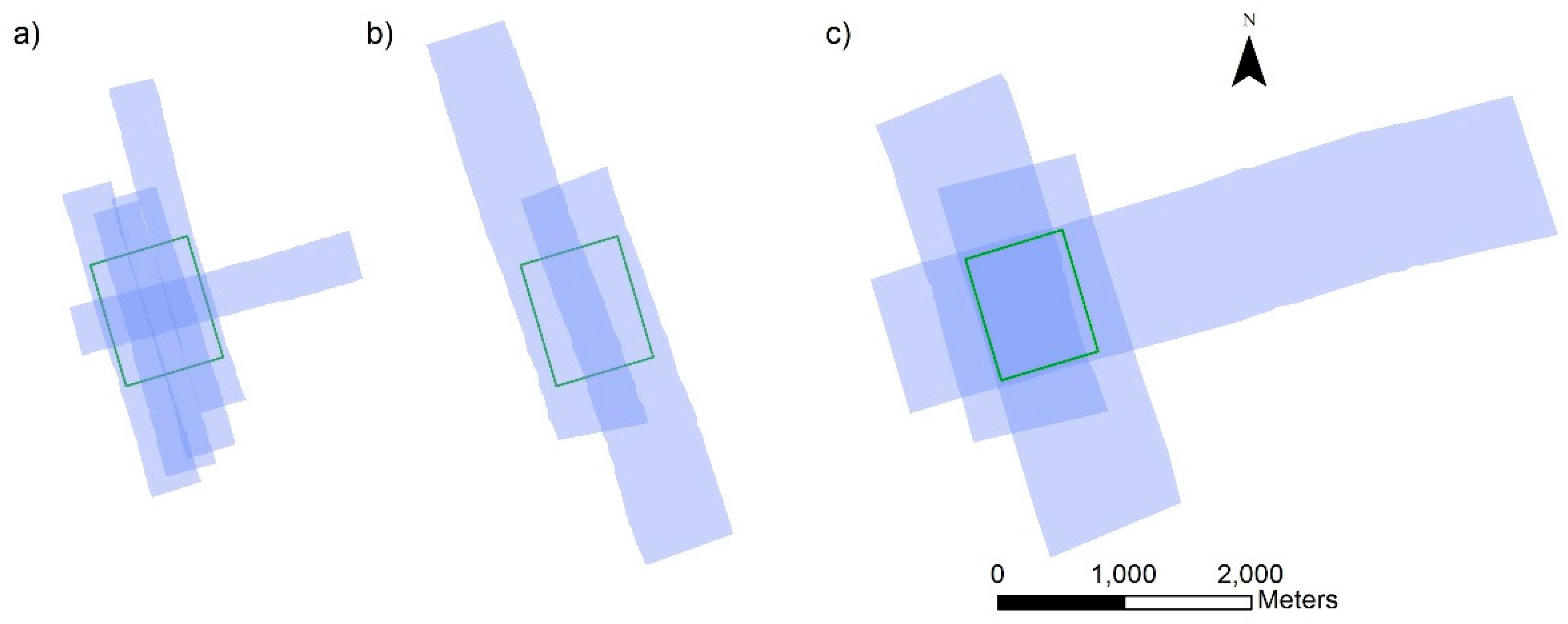
Discrete return lidar data were collected at three wavelengths (532 nm, 1064 nm, and 1550 nm) using the multi-spectral Teledyne Optech Titan system on 28 July, 2016 at flying altitudes of 500 m, 1000 m, and 1500 m AGL over a rural area in south-east Ontario (near the town of Warkworth), characterized by field crops, forest stands, open pasture, roads, and houses (Figure 1). This site was chosen due to the authors having access to the farm land property to assess land covers, and the location being sufficiently far from any other air traffic to enable loitering over the AOI at multiple altitudes. The data were collected at 75 kHz per channel and with a scan angle of +/−20 degrees. Scan frequencies (40 Hz, 38 Hz, and 32 Hz) varied with flying altitude (500 m, 1000 m, and 1500 m, respectively) to maintain a reasonably uniform sampling distribution. Altogether, ten swaths were collected – five at 500 m, two at 1000 m, and three at 1500 m (Table 1 and Figure 2). Sensor characteristics are presented in the Table 1. The relationship between the received power and the recorded intensities was said to be linear over the entire scale (pers.comm. Paul LaRoque, Teledyne Optech, 28 October, 2015). In addition, for channel 2 (1064 nm), a fraction of each outgoing pulse and the return pulse were recorded by a waveform digitizer at 1ns sampling interval.
Raw data in the form of a range file and a SBET file (smoothed best estimate trajectory) were processed in LMS (Lidar Mapping Suite, proprietary software from Teledyne Optech) and, after block adjustment, point cloud data were obtained with verified accuracy of RMS < 0.06 m in horizontal separation and RMS < 0.02 m in height separation (LMS report).
2.2. Scan Line Intensity Banding
During preliminary analysis, it was found that intensity values differed based on the mirror scan direction of the system. As explained in [49], the effect was due to a slight optical misalignment of the system, and its amplitude differs with flight altitude, maximum scan angle and scan frequency. As our study deals with system radiometry, half of the available data were therefore omitted in the radiometric analysis, but for spatial or geometric products all data were used. Thus, the ground pattern for our radiometric data became similar to a rotating polygon scanning system with halved data density.
2.3. Comparative Analysis
Lidar data were outputted from LMS in LAS format with intensities normalized to a range of 1000 m. For radiometric analysis, two types of intensity raster grids of 4 m × 4 m were created with LAStools (rapidlasso GmbH [50]) for each channel and each flight altitude from normalized to range DN intensity values (note, only one scan direction was used to avoid the banding issue) one raster grid was calculated by averaging intensity of all returns inside the grid cell, and the second raster grid was calculated by including only single returns and represents averaged-over-grid cell single returns’ intensity. These products were used for comparative analysis in the forms of different ratios, as explained below.
2.3.1. Point Density
Point density raster grids of 2 m × 2 m were calculated with LAStools (rapidlasso GmbH) for each channel and each altitude separately (note, both scan directions were used for this calculation). For the full AOI analysis, a summary table was filled with point densities, and numbers of returns, separated by return type. In addition, point densities of single returns over different vegetation classes (Figure 1a) were compared to point densities of all returns.
2.3.2. Single Channel Ratios
From intensity raster grids, single channel ratio grids were calculated with ArcGIS Spatial Analyst (ArcMap, ESRI), separately for all returns and for single returns for two combinations—intensity at 500 m divided by intensity at 1000 m, and intensity at 500 m divided by intensity at 1500 m.
Intensity values from lidar points from the virtual hay stubble plot normalized to range, and further normalized to the cosine of incidence angle, were compared to evaluate laser power stability. For channel 2, digitized outgoing pulse waveforms were sampled (21 per flight line) from pulses emitted over the virtual hay stubble plot. For each waveform, the noise level (Noise) was determined by averaging the first five readings sampled well before the leading edge of the pulse. This noise level was subtracted from the maximum sampled by the digitizer value (MaxDigiDN) for each waveform. (Note: MaxDigiDN should not be confused with the true peak value of the waveform, because some fitting algorithm would be necessary to derive the latter.) The resulting distributions of MaxDigiDN-minus-Noise values were compared for flight lines 3 and 4 (500 m), 6 and 7 (1000 m), 8 and 9 (1500 m).
2.3.3. Spectral Vegetation Indices Maps
Two types of SVI maps were generated with Spatial Analyst (ArcMap, ESRI) for three normalized difference indices nδ(C2, C3), nδ(C2, C1), and nδ(C1, C3), together with corresponding simple ratios, for each altitude—from averaged-all intensity raster grids and from averaged single return intensity raster grids.
2.3.4. Spectral Vegetation Indices Ratios
Analogous to single channel ratios, SVI to SVI ratios at different altitudes were calculated for single return intensity products. Raster histograms were outputted for ratios SVI (500 m)/SVI (1000 m), limiting the range of visualized values in such a way that outliers were not included. Histograms allow qualitative comparisons of simple ratio versus normalized difference products derived from Titan sensor intensity DNs normalized to range.
3. Results
3.1. Point Density Maps
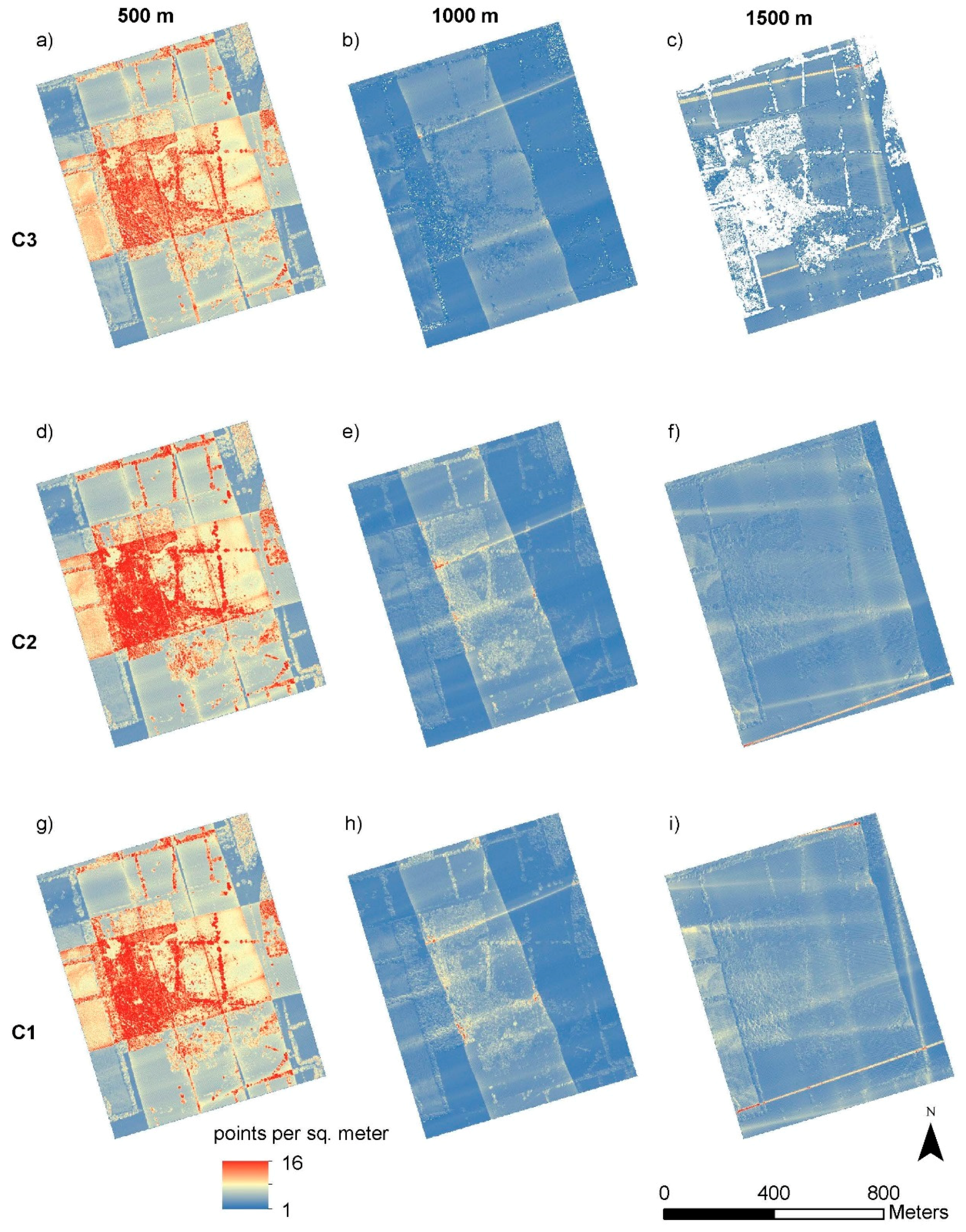
Table 2 presents a summary of the whole dataset. Figure 3 features density maps for all channels and altitudes separately (note cross line 5 at 500 m AGL vivid on maps a), d), and g)). Wide patterns of higher density on maps b), e), and i) corresponded to swath overlaps and narrow patterns of higher density on the same maps, together with ones on the maps c), f), and j) are due to aircraft attitude variation (e.g., rapid pitch change) during the survey. Most noticeable are white (‘no data’) pixels inside the AOI over the majority of the vegetated areas on map c), which corresponded to C3 channel at 1500 m survey altitude. In addition, some empty pixels appeared over vegetated areas on the map b) C3 channel at 1000 m.
Table 3 presents a comparison of point densities obtained from single returns to those obtained from all returns for different vegetation classes (Figure 1a). First, it is evident that C3 (532 nm) does not provide enough returns at 1500 m for single or all return products. Second, point density of single returns was always lower than for all returns and was between 0.9 and 3.6 points per sq. meter for all classes aside from the crop class. Last, for the crop class, the lowest single return point density was 0.4 points per sq. meter (C1 at 1000 m) and roughly equaled one third of the point density for all returns.
3.2. Single Channel Intensity Ratios
The results of the transmitter optical power stability analysis are presented in Figure 4 and Table 4. Figure 4 shows boxplots for MaxDigiDN-minus-Noise values of samples of outgoing pulses for lines L3 and L4 (at 500 m), L6 and L7 (at 1000 m), and L8 and L9 (at 1500 m) for channel C2 (1064 nm); the mean (and SD) values were 295.0 (7.8), 293.8 (5.6), 293.0 (5.3), 295.4 (6.0), 288.0 (4.5), and 290.2 (4.5) respectively. There was a statistically significant difference between lines as determined by one-way ANOVA test (p < 0.01). However, the paired T-test showed no statistically significant difference between L3 and L4 (p = 0.59), L6 (p = 0.33), L7 (p = 0.83), and significant difference (p < 0.01) in comparing L3 with L8 and L9; there was no significant difference between L8 and L9 (p = 0.19). The difference in means between L3 and L8 (maximum difference among lines) equaled to 7.0, which is 2.4%.
Table 4 summarizes the comparison of intensities normalized to range (), and additionally normalized to the cosine of incidence angle () for the same altitudes for a virtual hay stubble plot (Figure 1a) for selected flight lines (Figure 2 and Table 1) for all channels. A Kolmogorov-Smirnov (KS) test was performed to compare (and separately ) from two flight lines at the same flight altitudes (note difference in range for each flight line). Single channel ratios for the same altitude presented for all altitudes and channels and compared to single channel ratios (average of two lines from 500 m divided by average of two lines at 1000 m or at 1500 m) for different altitudes.
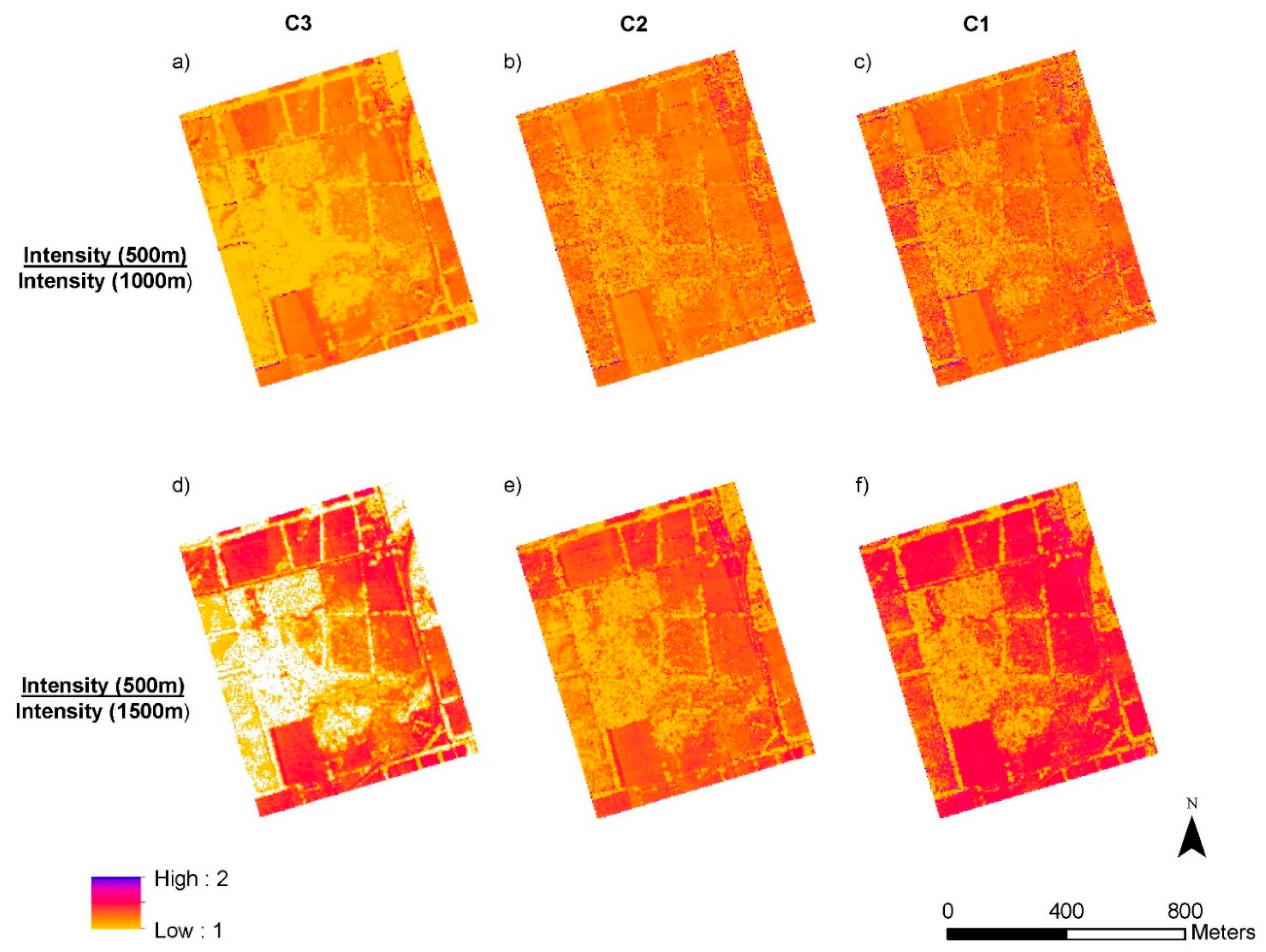
Maps, resulting from calculating single-channel ratios, are presented in Figure 5 and Figure 6. Lower values of pixels over vegetated areas were noted for all-returns maps (Figure 5) in comparison to values of extended surfaces (fields), and different results for single-return maps (Figure 6) higher ratio values for vegetated areas in comparison to fields. Table 5 provides the mean values and standard deviations for the images in Figure 5 and Figure 6, together with p-values of significant difference from the mean value equal to one for each distribution (95% confidence interval). In addition, p-values of two-sample Mann-Whitney test for comparing all-returns versus single-returns are presented (95% confidence interval).
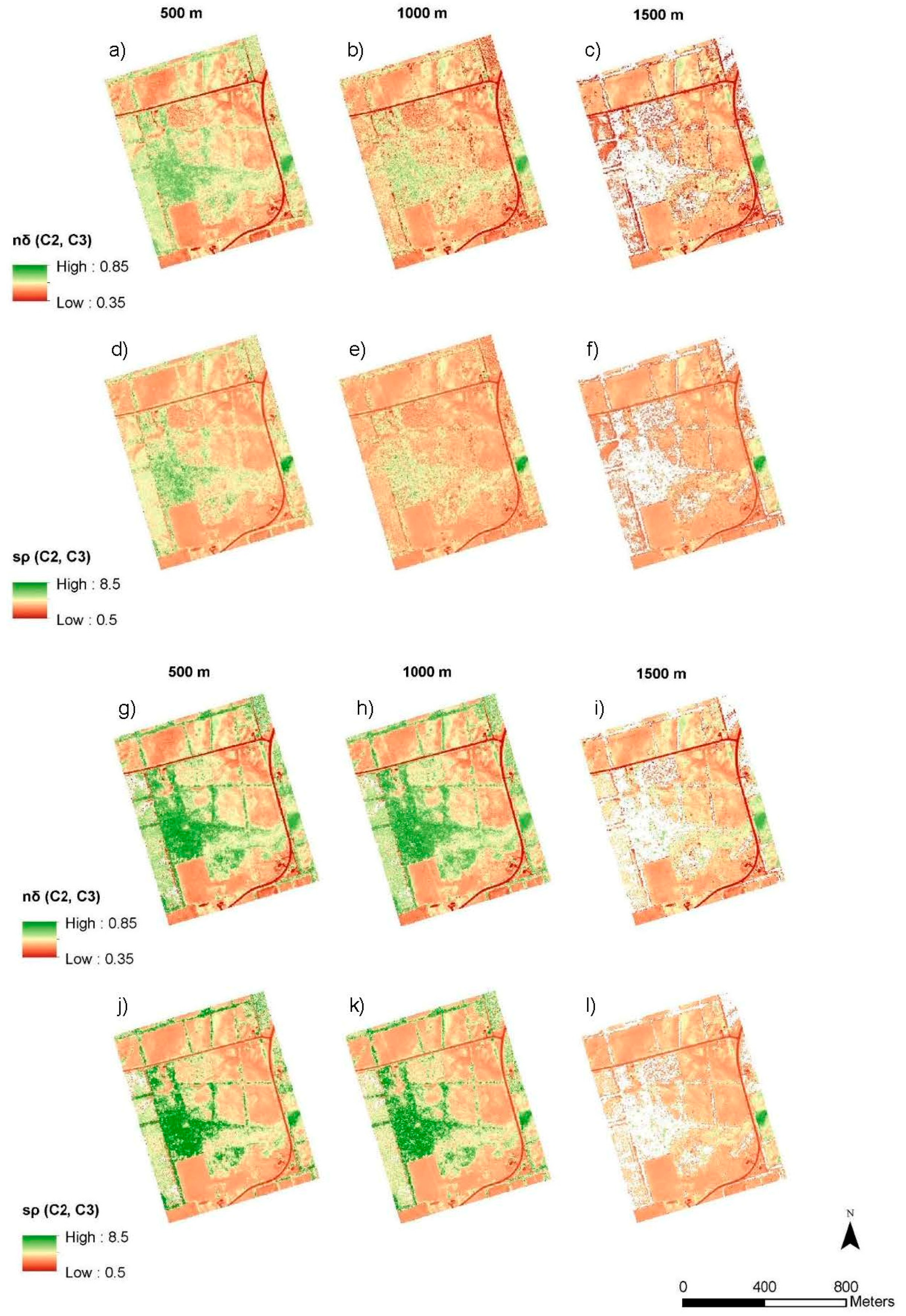
3.3. Spectral Vegetation Indices Maps
In Figure 7, there are two types of normalized difference maps compared to corresponding simple ratios for channels C2 and C3 for each altitude. Figure 7a–f were derived from all returns and Figure 7g–l were derived from single returns. Maps in Figure 7 are colored with a +/− two standard deviation color ramp based on values derived from maps g and j for nδ-maps and for sρ-maps, respectively. The similarities over extended targets (e.g., fields) were noted throughout all maps, consistency of values corresponding to vegetated areas on single-returns indices’ maps, and differences in pixel values of the same indices over the vegetated areas on maps derived from all returns. Table 6 shows the mean and standard deviation values for each image from Figure 7 and results of two-sample Kolmogorov—Smirnov tests of normalized differences and spectral ratios at 1000 m and 1500 m were compared to those at 500 m in the form of D-values and p-values. Note, all p-values were lower than 0.01 due to the large sample size (~80,000) and do not represent practical significance [51]. However, D-statistics of the test—the maximum distance between cumulative distribution functions—showed larger values for all returns (e.g., 0.19 for C2C3 at 1000 all) in comparison to single returns (0.02 for C2C3 at 1000 m singles).
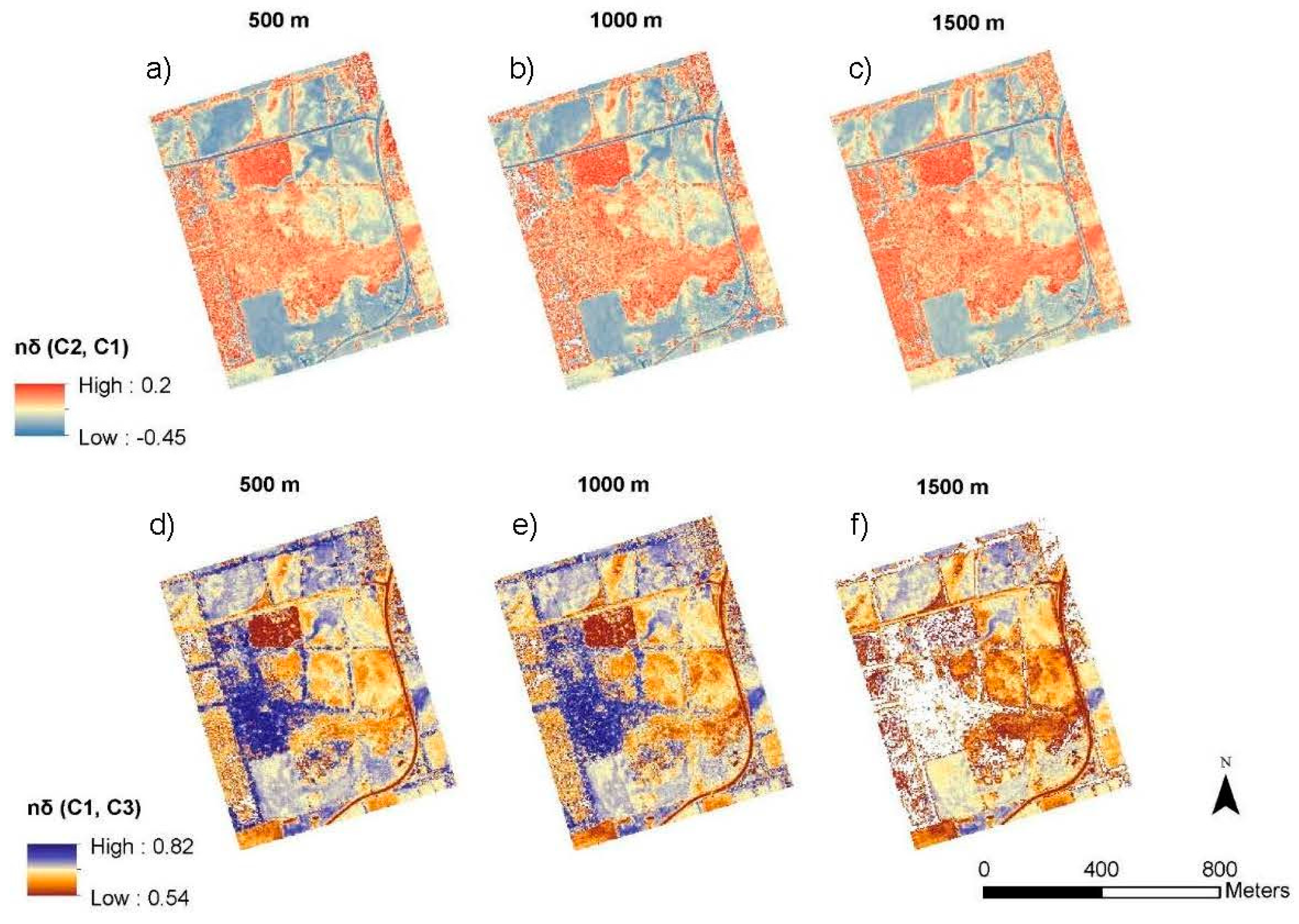
In Figure 8, there are nδ-maps of single returns for C1C2 and C1C3 combinations. The color scheme is similar to the one on Figure 7—it is colored with a +/− two standard deviation color ramp based on values derived from the map on Figure 8a for C1C2 maps, and from the map on Figure 8d for C1C3 maps. Note, there are nil nodata grid cells in the nδ(C1C2) map at 1500 m which was due to good point density at 1500 m for these channels (Figure 3f,i).
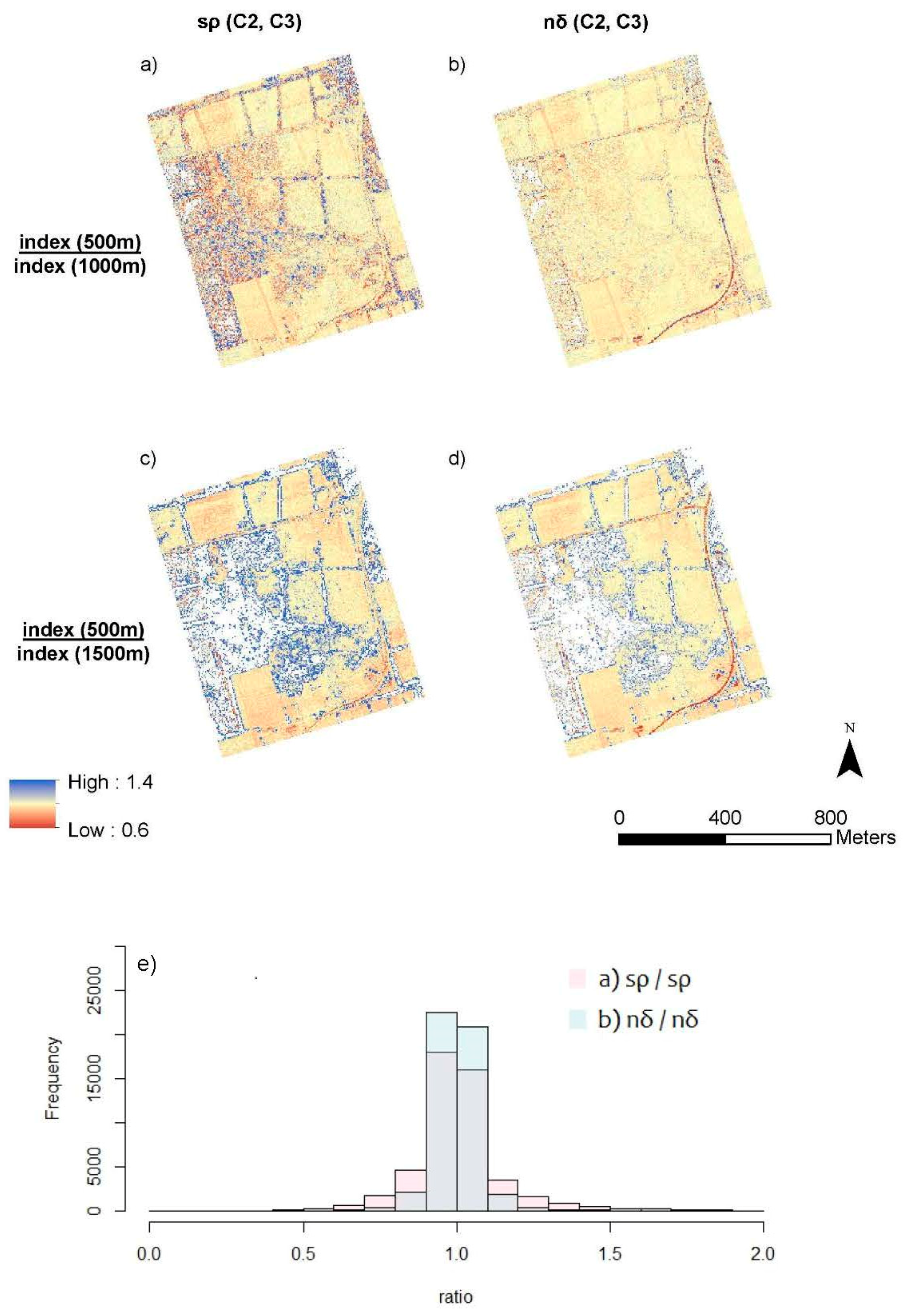
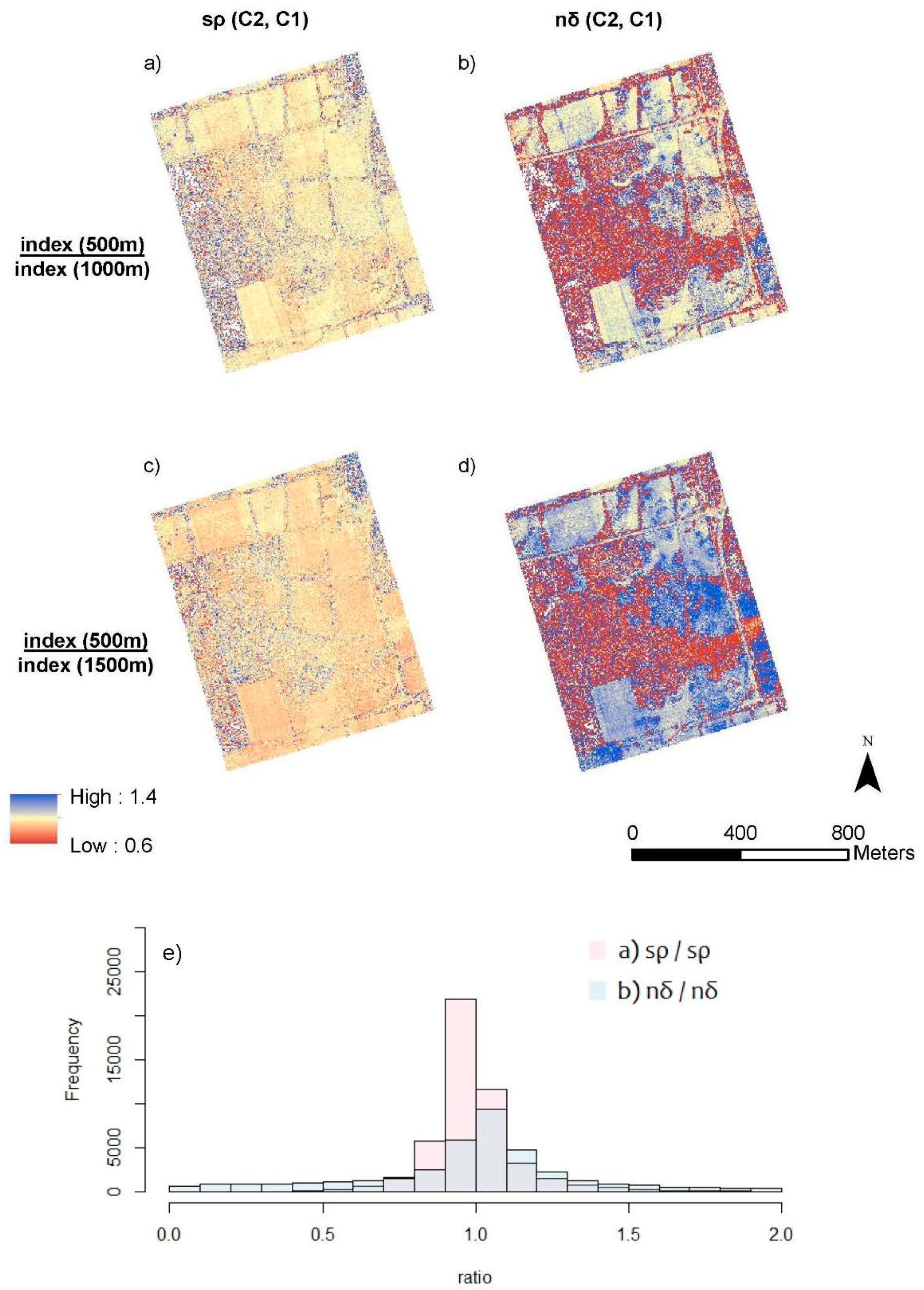
3.4. SVI Altitude Ratio Maps and Histograms
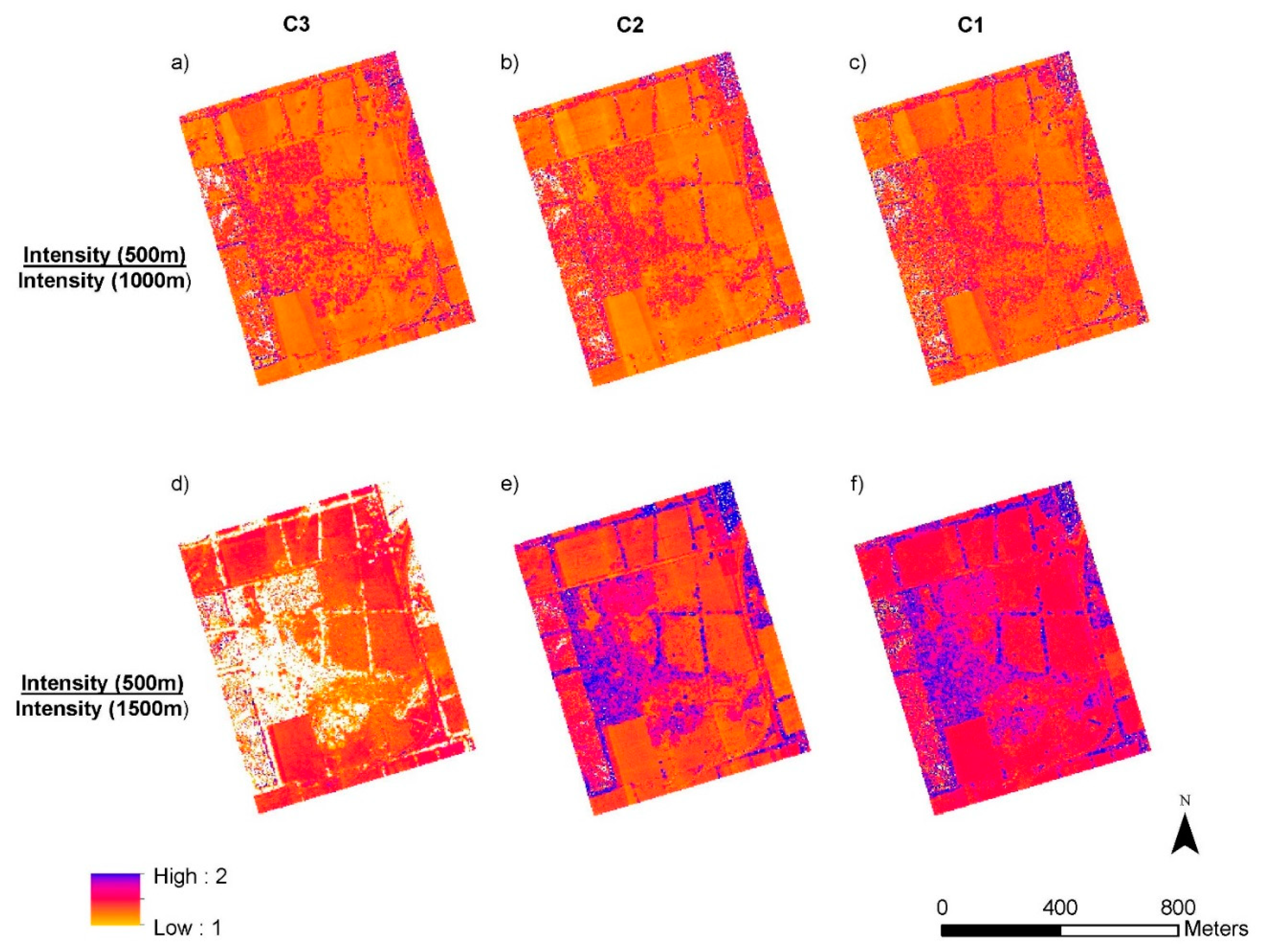
Figure 9, Figure 10 and Figure 11 show maps of SVIi (500 m)/SVIi (1000 m) with the corresponding histograms for images, and maps of SVIi (500 m)/SVIi (1500 m) derived from single returns. The color ramp for all images is based on +/− two standard deviations of sρ (500 m)/sρ (1000 m) images. The ratio range for all histograms is from 0.0 to 2.0. Table 7 shows the mean, standard deviation, min, and max values for each image from Figure 9, Figure 10 and Figure 11.
4. Discussion
From Table 5, it is evident, and as expected from Equation (17), that the inverse square range normalization alone does not normalize intensity DNs from different altitudes to equivalent values. While this can be a combination of two factors, transmitter power stability and atmospheric losses, from Table 4 and Figure 4 it is clear, that the major driver of the two was atmospheric loss, and additional atmospheric correction was needed. Transmitter power stability detected by the digitizer was within 2% for C2 (1064 nm), maximum variations to up to +/− 5% (Figure 6). Comparison of the flight lines at the same planned altitude confirmed the expected variations from [47] of ~ 4% for C2 and C3, and ~ 6% for C1 at altitudes 500 m and 1500 m. Larger variations (up to 9%) obtained at 1000 m altitude (L6 vs. L7) are likely due to the ~ 100 m difference in range for these two lines and the associated additional atmospheric losses. However, digitizing a portion of the outgoing pulse for each channel would provide better control over optical power stability, and additional radiometric calibration targets would allow separating effects due to atmospheric losses from power stability more clearly.
Furthermore, in Table 5, averages from all-return ratios are smaller in comparison to averages from single-return ratios. Moreover, from Figure 5 and Figure 6, it is obvious that ratios over vegetated areas increased in all-return ratio maps and decreased in single-return ratio maps in comparison to extended-target areas (e.g., hay stubble field). This effect can be explained by referring to the data in Table 2: with higher altitudes, the proportion of multiple returns decreased (i.e., more single returns). Multiple returns are, mainly, characteristic of tall vegetated areas. Thus, with ratios of average-of-all-returns, it was likely dividing intensity averaged over more returns from one pulse by intensity averaged over fewer returns from one pulse. If in Equation (17), the extended targets were substituted with point targets and it was assumed that only one emission-pulse was hitting the grid cell at nadir at two altitudes, then the average intensity at higher altitude would be higher due to fewer returns per one emitted pulse (Table 2). The average-of-all multiple return intensities is not purely a spectral characteristic and such a metric cannot be compared through different areas inside the same raster as a spectral value (e.g., vegetation canopy versus extended targets). In contrast, intensities derived from single returns, provided sufficient point density (Table 3), tend to possess a more reliable and consistent spectral characteristic of the target. With increasing altitude, the lidar backscatter signal weakened over vegetated areas to a greater degree than for extended target areas. This observation can be explained by the temporal elongation of the lidar backscatter response within tall vegetation, and an associated increase in the proportion of backscatter below the system detection threshold (i.e., a reduction in return signal below the noise floor).
From Figure 3, the green (532 nm) channel produced little energy backscatter from vegetation at 1500 m (in contrast to 1064 nm and 1550 nm), due to no return signal above the noise level. Moreover, the proportion of split-returns decreased (Table 2) with survey altitude for the Titan sensor. Given the tendency for lidar acquisition contracts to specify minimum return point densities, this observation justifies proposing an altitude threshold criterion at which the point density from vegetation is equal to that from a solid surface (or emission pulse density). Below this threshold altitude, vegetation would have higher point density than extended targets (solid surface), and above this altitude, vegetation would display lower point densities than extended targets. This concept is illustrated in Table 8 with approximate values from the Warkworth dataset.
From Figure 7 and Figure 8, it is evident that spectral ratio maps displayed visibly consistent patterns and ratio values over extended target areas. However, maps derived from single returns are more consistent (smaller values of D statistics from the Kolmogorov-Smirnov test in Table 6) in comparison to maps derived from averages-of-all returns—the difference is evident in vegetated areas (Figure 1a shows delineated areas of vegetation). It can be seen that both sρ and nδ indices exhibited the same spatial patterns. This indicates that for vegetated areas, SVIs derived from single returns over vegetated areas might be of more practical use, provided enough point density (Table 3), than those derived from averaged all return intensity metrics. A similar result was reported in [52] after the implementation of a random forest technique for selecting the most useful ms lidar spectral metrics in individual tree species classification.
9—11 show that the choice of the most consistent SVI between sρ and nδ indices were wavelength dependent. Contrary to our expectation from Equations (26) and (27), nδ(C2,C3) and nδ(C1,C3) were superior over sρ(C2,C3) and sρ(C1,C3). However, in the case of the C1 and C2 combination, the spectral ratio sρ(C2,C1) was more consistent in comparison to nδ(C2,C1). This result is in line with the work of [53] in which the authors concluded that nδ(C2,C1) (NDVINIR-MIR in the author’s notation) was the noisiest index among Titan’s normalized differences. The reason for this result might be in the type of the land cover—the average simple ratio of C2 and C1 channels for the AOI was ~0.8, while simple ratios of C2 and C3, and C1 and C3 combinations were ~4.5 and ~5.5 (Table 6). The channel dependent differences in atmospheric attenuation with altitude may lead to a change in intensity response from the scene, while the normalized difference may be oversensitive in areas where reflectance of C1 and C2 channels are close to each other. Thus, while it is possible to use combinations of nδ(C2,C3), nδ(C1,C3) and sρ(C2,C1) indices for interpretation and basic classification purposes, such as vegetation and land-cover within an urban environment, it is recommended to combine all three laser channels for more sophisticated classification needs (e.g., Hopkinson et al. [5]).
5. Conclusions
It has been shown that atmospheric correction is needed to compare intensity DN values at different ranges and development of the atmospheric correction model is a next logical step. A simple optical power stability analysis was performed showing consistency of ~ 4–6% for Teledyne Optech Titan sensor in this study. However, more rigorous control is recommended to further improve radiometric products. From the point density analysis, it became clear that the survey at 1500 m AGL with the Titan sensor did not provide enough lidar backscatter for the C3 channel over forest canopy areas. A survey altitude threshold criterion was proposed that may bring better comparability of datasets collected by different sensors and/or by the same sensor over different times and locations. It was shown, that SVI products derived from single-returns (provided sufficient point density) were more consistent across three altitudes over vegetated areas in comparison to SVIs derived from all returns. After comparing the stability of SVIs through different altitudes, it is recommended to use the combination of nδ(C2,C3), nδ(C1,C3) and sρ(C2,C1) indices for further analysis and classification of ms lidar point clouds. The next logical step in studying radiometry of ms lidar sensors is radiometric correction [45] which can be achieved by using ground reflectance targets (e.g., [46,47]).
Author Contributions
Conceptualization, C.H. and M.O.; methodology, C.H. and M.O.; software, C.H.; formal analysis, M.O.; resources, C.H.; data curation, C.H. and M.O.; writing—original draft preparation, M.O.; writing—review and editing, C.H. and M.O.; visualization, M.O.; supervision, C.H.; project administration, C.H.; funding acquisition, C.H. and M.O.
Funding
Okhrimenko acknowledges funding from Alberta Innovates Technology Futures. Hopkinson acknowledges funding from Canada Foundation for Innovation, NSERC, and Alberta Economic Development & Trade.
Acknowledgments
Teledyne Optech is gratefully acknowledged for providing the ms lidar sensor for the airborne missions along with Mike Sitar and Paul LaRocque for their constant help and support. Craig Coburn, Derek Peddle, Locke Spencer, Laura Chasmer, David McCaffrey, and Craig Mahoney acknowledged for useful discussions and friendly critique.
Conflicts of Interest
The authors declare no conflicts of interest.
References
- Vosselman, G.; Maas, H. Airborne and Terrestrial Laser Scanning; CRC Press: Boca Raton, FL, USA, 2010. [Google Scholar]
- Lu, D.; Mausel, P.; Brondizio, E.; Moran, E. Change detection techniques. Int. J. Remote Sens. 2004, 25, 2365–2407. [Google Scholar] [CrossRef]
- Lyon, J.G.; Yuan, D.; Lunetta, R.S.; Elvidge, C.D. A change detection experiment using vegetation indices. Photogramm. Eng. Remote Sens. 1998, 64, 143–150. [Google Scholar]
- Pettorelli, N. The Normalized Difference Vegetation Index; Oxford University Press: Oxford, UK, 2013. [Google Scholar]
- Hopkinson, C.; Chasmer, L.; Gynan, C.; Mahoney, C.; Sitar, M. Multisensor and Multispectral LiDAR Characterization and Classification of a Forest Environment. Can. J. Remote. Sens. 2016, 42, 501–520. [Google Scholar] [CrossRef]
- Baret, F.; Guyot, G. Potentials and Limits of Vegetation Indexes for Lai and Apar Assessment. Remote Sens. Environ. 1991, 35, 161–173. [Google Scholar] [CrossRef]
- Huete, A.R. Soil and Sun angle interactions on partial canopy spectra. Int. J. Remote. Sens. 1987, 8, 1307–1317. [Google Scholar] [CrossRef]
- Jackson, R.D.; Slater, P.N.; Pinter, P.J. Discrimination of Growth and Water-Stress in Wheat by Various Vegetation Indexes through Clear and Turbid Atmospheres. Remote Sens. Environ. 1983, 13, 187–208. [Google Scholar] [CrossRef]
- Zhang, Y.; Chen, J.M.; Miller, J.R.; Noland, T.L. Leaf chlorophyll content retrieval from airborne hyperspectral remote sensing imagery. Remote Sens. Environ. 2008, 112, 3234–3247. [Google Scholar] [CrossRef]
- Gaulton, R.; Danson, F.; Ramírez, F.; Gunawan, O.; Danson, F. The potential of dual-wavelength laser scanning for estimating vegetation moisture content. Remote. Sens. Environ. 2013, 132, 32–39. [Google Scholar] [CrossRef]
- Morsdorf, F.; Nichol, C.; Malthus, T.; Woodhouse, I.H. Assessing forest structural and physiological information content of multi-spectral LiDAR waveforms by radiative transfer modelling. Remote. Sens. Environ. 2009, 113, 2152–2163. [Google Scholar] [CrossRef] [Green Version]
- Hakala, T.; Nevalainen, O.; Kaasalainen, S.; Mäkipää, R. Technical Note: Multispectral lidar time series of pine canopy chlorophyll content. Biogeosciences 2015, 12, 1629–1634. [Google Scholar] [CrossRef]
- Rees, W.G. Physical Principles of Remote Sensing, 2nd ed.; Cambridge University Press: Cambridge, UK, 2004. [Google Scholar]
- Perry, C.R.; Lautenschlager, L.F. Functional Equivalence of Spectral Vegetation Indexes. Remote Sens. Environ. 1984, 14, 169–182. [Google Scholar] [CrossRef]
- Rouse, J., Jr.; Haas, R.H.; Schell, J.A.; Deering, D.W. Monitoring Vegetation Systems in the Great Plains with ERTS; NASA Special Publication: Washington, DC, USA, 1974; p. 351. [Google Scholar]
- Fernandez-Diaz, J.C.; Carter, W.E.; Glennie, C.; Shrestha, R.L.; Pan, Z.; Ekhtari, N.; Singhania, A.; Hauser, D.; Sartori, M. Capability Assessment and Performance Metrics for the Titan Multispectral Mapping Lidar. Remote. Sens. 2016, 8, 936. [Google Scholar] [CrossRef]
- Gates, D.M.; Keegan, H.J.; Schleter, J.C.; Weidner, V.R. Spectral Properties of Plants. Appl. Opt. 1965, 4, 11–20. [Google Scholar] [CrossRef]
- Gamon, J.A.; Serrano, L.; Surfus, J.S. The photochemical reflectance index: An optical indicator of photosynthetic radiation use efficiency across species, functional types, and nutrient levels. Oecologia 1997, 112, 492–501. [Google Scholar] [CrossRef] [PubMed]
- Gamon, J.; Peñuelas, J.; Field, C. A narrow-waveband spectral index that tracks diurnal changes in photosynthetic efficiency. Remote. Sens. Environ. 1992, 41, 35–44. [Google Scholar] [CrossRef]
- Hardisky, M.A.; Klemas, V.; Smart, R.M. The Influence of Soil-Salinity, Growth Form, and Leaf Moisture on the Spectral Radiance of Spartina-Alterniflora Canopies. Photogramm. Eng. Remote Sens. 1983, 49, 77–83. [Google Scholar]
- Hunt, E.R.; Rock, B.N. Detection of Changes in Leaf Water-Content Using near-Infrared and Middle-Infrared Reflectances. Remote Sens. Environ. 1989, 30, 43–54. [Google Scholar]
- Hancock, S.; Gaulton, R.; Danson, F.M. Angular Reflectance of Leaves with a Dual-Wavelength Terrestrial Lidar and Its Implications for Leaf-Bark Separation and Leaf Moisture Estimation. IEEE Trans. Geosci. Remote. Sens. 2017, 55, 1–7. [Google Scholar] [CrossRef]
- Chasmer, L.E.; Hopkinson, C.D.; Petrone, R.M.; Sitar, M. Using Multitemporal and Multispectral Airborne Lidar to Assess Depth of Peat Loss and Correspondence with a New Active Normalized Burn Ratio for Wildfires. Geophys. Res. Lett. 2017, 44. [Google Scholar] [CrossRef]
- Xu, H.Q. Modification of normalised difference water index (NDWI) to enhance open water features in remotely sensed imagery. Int. J. Remote Sens. 2006, 27, 3025–3033. [Google Scholar] [CrossRef]
- Morsy, S.; Shaker, A.; El-Rabbany, A.; Larocque, P.E. Airborne multispectral lidar data for land-cover classification and land/water mapping using different spectral indexes. ISPRS Ann. Photogramm. Remote. Sens. Spat. Inf. Sci. 2016, 3, 217–224. [Google Scholar] [CrossRef]
- Schott, J.R. Remote Sensing: The Image Chain Approach, 2nd ed.; Oxford University Press: Oxford, UK, 2007. [Google Scholar]
- Jelalian, A. Laser Radar Systems; Artech House: Norwood, MA, USA, 1992. [Google Scholar]
- Wagner, W. Radiometric calibration of small-footprint full-waveform airborne laser scanner measurements: Basic physical concepts. ISPRS J. Photogramm. Remote. Sens. 2010, 65, 505–513. [Google Scholar] [CrossRef]
- Baltsavias, E. Airborne laser scanning: Basic relations and formulas. ISPRS J. Photogramm. Remote. Sens. 1999, 54, 199–214. [Google Scholar] [CrossRef]
- Hopkinson, C. The influence of flying altitude, beam divergence, and pulse repetition frequency on laser pulse return intensity and canopy frequency distribution. Can. J. Remote. Sens. 2007, 33, 312–324. [Google Scholar] [CrossRef]
- Yan, W.Y.; Shaker, A.; El-Ashmawy, N. Urban land cover classification using airborne LiDAR data: A review. Remote. Sens. Environ. 2015, 158, 295–310. [Google Scholar] [CrossRef]
- Korpela, I.; Tuomola, T.; Tokola, T.; Dahlin, B. Appraisal of seedling stand vegetation with airborne imagery and discrete-return LiDAR—An exploratory analysis. Silva Fenn. 2008, 42, 753–772. [Google Scholar] [CrossRef]
- Hopkinson, C.; Chasmer, L. Testing LiDAR models of fractional cover across multiple forest ecozones. Remote. Sens. Environ. 2009, 113, 275–288. [Google Scholar] [CrossRef]
- García, M.; Riaño, D.; Chuvieco, E.; Danson, F.M. Estimating biomass carbon stocks for a Mediterranean forest in central Spain using LiDAR height and intensity data. Remote. Sens. Envtron. 2010, 114, 816–830. [Google Scholar] [CrossRef]
- Holmgren, J.; Persson, Å. Identifying species of individual trees using airborne laser scanner. Remote. Sens. Environ. 2004, 90, 415–423. [Google Scholar] [CrossRef]
- Donoghue, D.N.; Watt, P.J.; Cox, N.J.; Wilson, J. Remote sensing of species mixtures in conifer plantations using LiDAR height and intensity data. Remote. Sens. Environ. 2007, 110, 509–522. [Google Scholar] [CrossRef]
- Korpela, I.; Ørka, H.; Maltamo, M.; Tokola, T.; Hyyppä, J. Tree species classification using airborne LiDAR—Effects of stand and tree parameters, downsizing of training set, intensity normalization, and sensor type. Silva Fenn. 2010, 44, 319–339. [Google Scholar] [CrossRef]
- Yan, W.Y.; Shaker, A.; Habib, A.; Kersting, A.P. Improving classification accuracy of airborne LiDAR intensity data by geometric calibration and radiometric correction. ISPRS J. Photogramm. Remote. Sens. 2012, 67, 35–44. [Google Scholar] [CrossRef]
- Roncat, A.; Morsdorf, F.; Briese, C.; Wagner, W.; Pfeifer, N. Laser Pulse Interaction with Forest Canopy: Geometric and Radiometric Issues. For. Appl. Airborne Laser Scanning: Concepts Case Stud. 2014, 27, 19–41. [Google Scholar]
- Wagner, W.; Ullrich, A.; Ducic, V.; Melzer, T.; Studnicka, N. Gaussian decomposition and calibration of a novel small-footprint full-waveform digitising airborne laser scanner. ISPRS J. Photogramm. Remote. Sens. 2006, 60, 100–112. [Google Scholar] [CrossRef]
- Nicodemus, F.E.; Richmond, J.C.; Hsia, J.J.; Ginsberg, I.W.; Limperis, T. Geometrical Considerations and Nomenclature for Reflectance; US Department of Commerce, National Bureau of Standards: Washington, DC, USA, 1977.
- Kukko, A.; Kaasalainen, S.; Litkey, P. Effect of incidence angle on laser scanner intensity and surface data. Appl. Opt. 2008, 47, 986. [Google Scholar] [CrossRef]
- Govaerts, Y.M.; Jacquemoud, S.; Verstraete, M.M.; Ustin, S.L. Three-dimensional radiation transfer modeling in a dicotyledon leaf. Appl. Opt. 1996, 35, 6585. [Google Scholar] [CrossRef] [PubMed]
- Li, Z.; Jupp, D.L.B.; Strahler, A.H.; Schaaf, C.B.; Howe, G.; Hewawasam, K.; Douglas, E.S.; Chakrabarti, S.; Cook, T.A.; Paynter, I.; et al. Radiometric Calibration of a Dual-Wavelength, Full-Waveform Terrestrial Lidar. Sensors 2016, 16, 313. [Google Scholar] [CrossRef]
- Kaasalainen, S.; Hyyppa, H.; Kukko, A.; Litkey, P.; Ahokas, E.; Hyyppa, J.; Lehner, H.; Jaakkola, A.; Suomalainen, J.; Akujarvi, A.; et al. Radiometric Calibration of LIDAR Intensity with Commercially Available Reference Targets. IEEE Trans. Geosci. Remote. Sens. 2009, 47, 588–598. [Google Scholar] [CrossRef]
- Okhrimenko, M.; Coburn, C.; Hopkinson, C. Investigating Multi-Spectral Lidar Radiometry: An Overview of the Experimental Framework. In Proceedings of the IGARSS 2018—2018 IEEE International Geoscience and Remote Sensing Symposium, Valencia, Spain, 23–27 July 2018; pp. 8745–8748. [Google Scholar]
- Okhrimenko, M.; Hopkinson, C. Multi-spectral lidar: Radiometric calibration, canopy reflectance, and vegetation vertical SVI profiles. Remote Sens. 2019, submitted. [Google Scholar]
- Steven, M.D.; Malthus, T.J.; Baret, F.; Xu, H.; Chopping, M.J. Intercalibration of vegetation indices from different sensor systems. Remote. Sens. Environ 2003, 88, 412–422. [Google Scholar] [CrossRef]
- Yan, W.Y.; Shaker, A. Airborne LiDAR intensity banding: Cause and solution. ISPRS J. Photogramm. Remote. Sens. 2018, 142, 301–310. [Google Scholar] [CrossRef]
- Isenburg, M. LAStools—Efficient LiDAR Processing Software. (Version 161029, Academic). 2016. Available online: http://rapidlasso.com/LAStools (accessed on 15 August 2016).
- Lin, M.F.; Lucas, H.C.; Shmueli, G. Too Big to Fail: Large Samples and the p-Value Problem. Inf. Syst. Res. 2013, 24, 906–917. [Google Scholar] [CrossRef]
- Budei, B.C.; St-Onge, B.; Hopkinson, C.; Audet, F.-A. Identifying the genus or species of individual trees using a three-wavelength airborne lidar system. Remote. Sens. Environ. 2018, 204, 632–647. [Google Scholar] [CrossRef]
- Morsy, S.; Shaker, A.; El-Rabbany, A.; Passaro, V.M.N. Multispectral LiDAR Data for Land Cover Classification of Urban Areas. Sensors 2017, 17, 958. [Google Scholar] [CrossRef] [PubMed]
Figure 1.
(a) The area of interest (AOI) with highlighted classes; (b) lidar point cloud colorized by passive RGB imagery. The thematic map was classified based on passive imagery and the familiarity of the field support team with the AOI. Virtual plots for a coniferous stand and a hay stubble field are 11.3 m radii circle areas chosen for additional analysis.

Figure 2.
Swath coverage of the AOI by lidar at altitudes: (a) 500 m; (b) 1000 m; (c) 1500 m.

Figure 3.
Point density maps from all returns at 2 m × 2 m grids. Top to bottom: C3, C2, and C1; left to right: 500 m, 1000 m, and 1500 m. White pixels represent no data. The explanation for density patterns is in the text.
Figure 3.
Point density maps from all returns at 2 m × 2 m grids. Top to bottom: C3, C2, and C1; left to right: 500 m, 1000 m, and 1500 m. White pixels represent no data. The explanation for density patterns is in the text.

Figure 4.
The boxplot showing maximum values (with subtracted noise) of the digitized fraction of an outgoing pulse for subsamples of 21 pulses per flight line over the virtual hay stubble plot for channel C2 (1064 nm).
Figure 4.
The boxplot showing maximum values (with subtracted noise) of the digitized fraction of an outgoing pulse for subsamples of 21 pulses per flight line over the virtual hay stubble plot for channel C2 (1064 nm).

Figure 5.
Single channels ratios of normalized to range 1000 m average intensity at 4 m × 4 m grid from all returns for each channel: Ci (500 m)/Ci (1000 m) in top figures, and Ci (500 m)/Ci (1500 m) in bottom figures. The channels are presented from left to right: C3, C2, and C1. White pixels represent no data.

Figure 6.
Single channels ratios of normalized to range 1000 m average intensity at 4 m × 4 m grid from single returns for each channel: Ci (500 m)/Ci (1000 m) in top figures, and Ci (500 m)/Ci (1500 m) in bottom figures. The channels are presented from left to right: C3, C2, and C1. White pixels represent no data.

Figure 7.
nδ (C2, C3) and sρ (C2, C3) for all returns (a–f) and single returns (g–l), averaged over 4 m × 4 m grid. White pixels represent no data.
Figure 7.
nδ (C2, C3) and sρ (C2, C3) for all returns (a–f) and single returns (g–l), averaged over 4 m × 4 m grid. White pixels represent no data.

Figure 8.
nδ (C2, C1) and nδ (C1, C3) for single returns, averaged over 4 m × 4 m grid. White pixels represent no data.
Figure 8.
nδ (C2, C1) and nδ (C1, C3) for single returns, averaged over 4 m × 4 m grid. White pixels represent no data.

Figure 9.
Ratios derived from single return indices at 4 m × 4 m grid: (a) ratio of sρ (C2, C3) at 500 m to sρ (C2, C3) at 1000 m; (b) ratio of nδ (C2, C3) at 500 m to nδ (C2, C3) at 1000 m; (c) Ratios of sρ (C2, C3) at 500 m to sρ (C2, C3) at 1500 m; (d) ratio of nδ (C2, C3) at 500 m to nδ (C2, C3) at 1500 m. (e) histograms for Figure 9a,b. White pixels represent no data.

Figure 10.
Ratios derived from single return indices at 4 m × 4 m grid: (a) ratio of sρ (C2, C1) at 500 m to sρ (C2, C1) at 1000 m; (b) ratio of nδ (C2, C1) at 500 m to nδ (C2, C1) at 1000 m; (c) Ratios of sρ (C2, C1) at 500 m to sρ (C2, C1) at 1500 m; (d) ratio of nδ (C2, C1) at 500 m to nδ (C2, C1) at 1500 m. (e) histograms for Figure 10a,b. White pixels represent no data.

Figure 11.
Ratios derived from single return indices at 4 m × 4 m grid: (a) ratios of sρ (C1, C3) at 500 m to sρ (C1, C3) at 1000 m; (b) ratio of nδ (C1, C3) at 500 m to nδ (C1, C3) at 1000 m; (c) Ratios of sρ (C1, C3) at 500 m to sρ (C1, C3) at 1500 m; (d) ratio of nδ (C1, C3) at 500 m to nδ (C1, C3) at 1500 m. (e) histograms for Figure 11a,b. White pixels represent no data.


Table 1.
Lidar parameters for each swath. *PRF (Pulse Repetition Frequency) is given for one channel.
Table 1.
Lidar parameters for each swath. *PRF (Pulse Repetition Frequency) is given for one channel.
| Flight Line (L) | L1 | L2 | L3 | L4 | L5 | L6 | L7 | L8 | L9 | L10 |
|---|---|---|---|---|---|---|---|---|---|---|
| <Range>, m | 491 | 540 | 547 | 546 | 536 | 942 | 1018 | 1475 | 1540 | 1555 |
| PRF*, kHz | 75 | 75 | 75 | 75 | 75 | 75 | 75 | 75 | 75 | 75 |
| SF, Hz | 40 | 40 | 40 | 40 | 40 | 38 | 38 | 32 | 32 | 32 |
| Swath, deg | 40.0 | 40.0 | 40.0 | 40.0 | 40.0 | 40.0 | 40.0 | 40.0 | 40.0 | 40.0 |
| <Speed>, m/s | 67 | 65 | 65 | 69 | 66 | 63 | 68 | 64 | 59 | 68 |
| Heading, deg | 160 | 340 | 160 | 340 | 250 | 160 | 340 | 160 | 340 | 250 |
Table 2.
Summary table of the Lidar dataset (note that statistics is given for all points in AOI).
| 500 m | 1000 m | 1500 m | |||||||
|---|---|---|---|---|---|---|---|---|---|
| C1/C2/C3 | C1 | C2 | C3 | C1 | C2 | C3 | C1 | C2 | C3 |
| Wavelength | 1550 nm | 1064 nm | 532 nm | 1550 nm | 1064 nm | 532 nm | 1550 nm | 1064 nm | 532 nm |
| Point density all | 8.05 | 8.35 | 7.57 | 2.55 | 2.57 | 1.9 | 3.14 | 2.85 | 2.38 |
| Point density last | 5.7 | 5.71 | 5.68 | 2 | 2 | 1.8 | 2.8 | 2.59 | 2.38 |
| Spacing all, cm | 0.35 | 0.35 | 0.36 | 0.63 | 0.62 | 0.73 | 0.56 | 0.59 | 0.65 |
| Number of returns | 6,468,902 | 6,709,651 | 6,083,545 | 2,050,152 | 2,059,638 | 1,502,604 | 2,525,347 | 2,291,578 | 1,337,302 |
| Footprint diameter at nadir, cm | 18 | 18 | 35 | 35 | 35 | 70 | 53 | 53 | 105 |
| Single | 3,269,931 | 3,151,688 | 3,344,283 | 1,236,739 | 1,231,412 | 1,347,771 | 1,984,104 | 1,887,007 | 1,336,696 |
| Double | 1,741,204 | 1,822,086 | 1,903,834 | 591,220 | 606,513 | 153,513 | 518,169 | 368,437 | 606 |
| Triple | 933,480 | 1,087,821 | 673,996 | 181,753 | 183,627 | 1,316 | 22,510 | 35,130 | 0 |
| Quadruple | 524,287 | 648,056 | 161,432 | 40,440 | 38,086 | 4 | 564 | 1,004 | 0 |
| First | 4,584,010 | 4,588,576 | 4,562,217 | 1,603,452 | 1,605,753 | 1,425,026 | 2,251,163 | 2,083,401 | 1,336,999 |
| Second | 1,312,320 | 1,435,277 | 1,216,281 | 366,052 | 373,756 | 77,137 | 266,407 | 195,979 | 303 |
| Third | 441,804 | 524,168 | 264,788 | 70,566 | 70,627 | 440 | 7,636 | 11,947 | 0 |
| Fourth | 130,768 | 161,630 | 40,259 | 10082 | 9502 | 1 | 141 | 251 | 0 |
Table 3.
Point density in points per square meter for lidar returns 0.5 m above ground for all returns and for single returns for different vegetation classes from Figure 1a. The density for the hay stubble class (i.e., ground) is presented for a reference to point density from extended targets.
Table 3.
Point density in points per square meter for lidar returns 0.5 m above ground for all returns and for single returns for different vegetation classes from Figure 1a. The density for the hay stubble class (i.e., ground) is presented for a reference to point density from extended targets.
| 500 m | 1000 m | 1500 m | |||||||
|---|---|---|---|---|---|---|---|---|---|
| C1/C2/C3 Wavelength, nm | C1 1550 | C2 1054 | C3 532 | C1 1550 | C2 1064 | C3 532 | C1 1550 | C2 1064 | C3 532 |
| Hay stubble | 5.3 | 5.35 | 5.0 | 2.5 | 2.4 | 2.0 | 3.2 | 2.9 | 2.6 |
| Coniferous all | 9.9 | 10.8 | 9.7 | 4.0 | 3.6 | 2.6 | 2.6 | 2.2 | 0.1 |
| Coniferous single | 3.4 | 2.7 | 3.6 | 2.0 | 1.5 | 2.1 | 2.2 | 1.5 | 0.1 |
| Deciduous all | 14.3 | 15.1 | 12.0 | 3.3 | 3.3 | 1.3 | 3.4 | 2.7 | <0.1 |
| Deciduous single | 2.3 | 1.9 | 3.2 | 0.9 | 0.9 | 1.1 | 2.0 | 1.6 | <0.1 |
| Mixed all | 12.7 | 14.0 | 11.4 | 3.7 | 3.8 | 1.8 | 3.0 | 2.6 | 0.1 |
| Mixed singles | 3.1 | 2.6 | 3.5 | 1.4 | 1.3 | 1.6 | 2.1 | 1.7 | 0.1 |
| Crop all | 5.0 | 5.2 | 5.1 | 1.3 | 1.6 | 1.3 | 2.7 | 2.3 | 0.2 |
| Crop singles | 1.1 | 1.0 | 0.8 | 0.4 | 0.6 | 0.8 | 1.1 | 1.5 | 0.2 |
Table 4.
The comparison of range and incidence angle normalized intensities for the same altitudes for a virtual hay stubble plot (Figure 1a) for selected flight lines (Table 1). KS test comparing range-normalized intensity from two flight lines at the same altitude (note difference in the Range column). The number of points (N) presented for each flight line and channel. The single channel ratios presented for all altitudes and channels and compared to single channel ratios for different altitudes.
| Range, m | C1 (1550 nm) | C2 (1064 nm) | C3 (532 nm) | |||||||
|---|---|---|---|---|---|---|---|---|---|---|
| N | N | N | ||||||||
| L3 | 515 | 580 | 772.2 (51.9) | 778,0 (54.0) | 486 | 394.0 (30.5) | 396.5 (30.7) | 556 | 136.6 (11.0) | 137.5 (11.1) |
| KS test | D = 0.133 p < 0.01 | D = 0.095 p = 0.012 | D = 0.132 p < 0.01 | D = 0.094 p = 0.018 | D = 0.038 p = 0.997 | D = 0.205 p < 0.01 | ||||
| L4 | 525 | 536 | 759.6 (52.7) | 790.2 (54.7) | 591 | 383.9 (28.6) | 389.4 (29.0) | 418 | 137.1 (10.8) | 142.3 (11.2) |
| L3/L4 | 1.07 | 0.98 | 1.03 | 1.02 | 1.00 | 1.00 | ||||
| L6 | 916 | 280 | 643.7 (41.6) | 646.8 (41.8) | 294 | 328.6 (22.7) | 330.2 (22.8) | 289 | 114.6 (8.2) | 115.0 (8.3) |
| KS test | D = 0.688 p < 0.01 | D = 0.544 p < 0.01 | D = 0.436 p < 0.01 | D = 0261 p < 0.01 | D = 0.630 p < 0.01 | D = 0.461 p < 0.01 | ||||
| L7 | 1023 | 253 | 571.3 (36.8) | 595.5 (38.0) | 266 | 304.6 (19.0) | 317.6 (19.8) | 290 | 102.3 (6.7) | 106.7 (7.0) |
| L6/L7 | 1.13 | 1.09 | 1.08 | 1.04 | 1.12 | 1.08 | ||||
| (L3+L4)/(L6+L7) | 1.26 | 1.26 | 1.23 | 1.21 | 1.26 | 1.26 | ||||
| L8 | 1460 | 250 | 553.4 (30.8) | 553.4 (30.8) | 218 | 301.5 (16.7) | 301.5 (16.7) | 881 | 100.8 (7.4) | 100.8 (7.4) |
| KS test | D = 0.506 p < 0.01 | D = 0.425 p < 0.01 | D = 0.330 p < 0.01 | D = 0.220 p < 0.01 | D = 0.233 p < 0.01 | D = 0.184 p < 0.01 | ||||
| L9 | 1514 | 212 | 514.1 (29.6) | 522.6(30.1) | 198 | 289.4 (16.7) | 294.3 (17.0) | 190 | 97.0 (7.1) | 98.7 (7.2) |
| L8/L9 | 1.08 | 1.06 | 1.04 | 1.02 | 1.04 | 1.02 | ||||
| (L3+L4)/(L8+L9) | 1.43 | 1.46 | 1.32 | 1.32 | 1.38 | 1.40 | ||||
Table 5.
The mean values and standard deviation for single-channel ratios for the whole AOI. One sample t-test (for the mean equals to one) p-values are given for 0.95 confidence interval. Two sample Mann-Whitney test p-values are given for 0.95 confidence interval.
Table 5.
The mean values and standard deviation for single-channel ratios for the whole AOI. One sample t-test (for the mean equals to one) p-values are given for 0.95 confidence interval. Two sample Mann-Whitney test p-values are given for 0.95 confidence interval.
| All Returns | Paired Test, p-Value | Single Returns | ||||||
|---|---|---|---|---|---|---|---|---|
| MEAN | SD | p | MEAN | SD | p | |||
| a) | C3(500 m)/C3(1000 m) | 1.08 | 0.20 | <0.01 | <0.01 | 1.31 | 0.23 | <0.01 |
| d) | C3(500 m)/C3(1500 m) | 1.14 | 0.30 | <0.01 | <0.01 | 1.30 | 0.18 | <0.01 |
| b) | C2(500 m)/C2(1000 m) | 1.19 | 0.15 | <0.01 | <0.01 | 1.31 | 0.23 | <0.01 |
| e) | C2(500 m)/C2(1500 m) | 1.20 | 0.17 | <0.01 | <0.01 | 1.51 | 0.33 | <0.01 |
| c) | C1(500 m)/C1(1000 m) | 1.22 | 0.20 | <0.01 | <0.01 | 1.34 | 0.27 | <0.01 |
| f) | C1(500 m)/C1(1500 m) | 1.29 | 0.20 | <0.01 | <0.01 | 1.60 | 0.33 | <0.01 |
Table 6.
The mean values and standard deviation (in brackets) for nδ and sρ for the whole AOI at three altitudes, derived from all returns and from single returns. P-values and D-statistics from Kolmogorov-Smirnov test are given for comparisons of 500 m products to 1000 m products, and 1500 m products. All p-values are low because of the large sample size (~80,000) and D-statistics provide values of practical significance for interpretation.
| Index | AGL, m | (C2,C3) | (C2,C1) | (C1,C3) | |||
|---|---|---|---|---|---|---|---|
| (1064 nm, 532 nm) | (1064 nm, 1550 nm) | (1550 nm, 532 nm) | |||||
| <all> | <single> | <all> | <single> | <all> | <single> | ||
| nδ | 500 | 0.57 (0.10) | 0.60 (0.12) | −0.14 (0.13) | −0.12 (0.16) | 0.66 (0.06) | 0.68 (0.07) |
| 1000 | 0.54 (0.09) D = 0.19, p < 0.01 | 0.60 (0.12) D = 0.02, p < 0.01 | −0.13 (0.14) D = 0.05, p < 0.01 | −0.11 (0.16) D = 0.03, p < 0.01 | 0.62 (0.08) D = 0.24, p < 0.01 | 0.67 (0.07) D = 0.03, p < 0.01 | |
| 1500 | 0.50 (0.09) D = 0.33, p < 0.01 | 0.54 (0.08) D = 0.31, p < 0.01 | −0.11 (0.13) D = 0.10, p < 0.01 | −0.09 (0.14) D = 0.11, p < 0.01 | 0.60 (0.10) D = 0.31, p < 0.01 | 0.62 (0.08) D = 0.26, p < 0.01 | |
| sρ | 500 | 3.91 (1.11) | 4.54 (2.03) | 0.78 (0.23) | 0.82 (0.27) | 5.12 (1.05) | 5.53 (1.60) |
| 1000 | 3.47 (0.85) D = 0.19, p < 0.01 | 4.49 (1.85) D = 0.02, p < 0.01 | 0.80 (0.23) D = 0.05, p < 0.01 | 0.84 (0.28) D = 0.03, p < 0.01 | 4.51 (1.09) D = 0.24, p < 0.01 | 5.42 (1.55) D = 0.03, p < 0.01 | |
| 1500 | 3.16 (0.75) D = 0.33, p < 0.01 | 3.44 (0.73) D = 0.31, p < 0.01 | 0.83 (0.21) D = 0.10, p < 0.01 | 0.87 (0.24) D = 0.11, p < 0.01 | 4.24 (1.17) D = 0.31, p < 0.01 | 4.49 (1.04) D = 0.26, p < 0.01 | |
Table 7.
The mean, standard deviation, min, and max values of each image from Figure 9, Figure 10 and Figure 11. Note, that all images for this comparison were derived from single returns.
| 500 m/1000 m | 500 m/1500 m | ||||||
|---|---|---|---|---|---|---|---|
| Mean(SD) | min | max | Mean(SD) | min | max | ||
| (C2,C3) | sρ | 1.02(0.20) | 0.15 | 10.10 | 1.13(0.40) | 0.29 | 11.13 |
| nδ | 1.00(0.62) | −11.95 | 130.06 | 1.05(0.33) | −35.06 | 28.14 | |
| (C2,C1) | sρ | 1.00(0.18) | 0.08 | 6.09 | 0.96(0.16) | 0.07 | 5.78 |
| nδ | 0.80(3.83) | −103.06 | 118.32 | 0.95(4.14) | −126.80 | 123.60 | |
| (C1,C3) | sρ | 1.03(0.21) | 0.08 | 12.68 | 1.21(0.41) | 0.16 | 12.30 |
| nδ | 1.01(0.09) | −5.92 | 8.43 | 1.09(0.22) | −15.81 | 12.07 | |
Table 8.
Point density m−2 of vegetated area in comparison to an open area (second value) at one flight line averaged over 11.3 m radii circle area (virtual plots in Figure 1a).
Table 8.
Point density m−2 of vegetated area in comparison to an open area (second value) at one flight line averaged over 11.3 m radii circle area (virtual plots in Figure 1a).
| 532 nm | 1064 nm | 1550 nm | |
| 500 m | ~ 4.2/2.4 | ~ 4.5/2.5 | ~4.2/2.4 |
| 1000 m | ~ 1.0 /1.3 | ~2.0/1.3 | ~ 2.1/1.3 |
| 1500 m | ~ 0.04/0.8 | ~0.8/0.8 | ~ 0.9/0.9 |
© 2019 by the authors. Licensee MDPI, Basel, Switzerland. This article is an open access article distributed under the terms and conditions of the Creative Commons Attribution (CC BY) license (http://creativecommons.org/licenses/by/4.0/).
Share and Cite
MDPI and ACS Style
Okhrimenko, M.; Hopkinson, C. Investigating the Consistency of Uncalibrated Multispectral Lidar Vegetation Indices at Different Altitudes. Remote Sens. 2019, 11, 1531. https://0-doi-org.brum.beds.ac.uk/10.3390/rs11131531
AMA Style
Okhrimenko M, Hopkinson C. Investigating the Consistency of Uncalibrated Multispectral Lidar Vegetation Indices at Different Altitudes. Remote Sensing. 2019; 11(13):1531. https://0-doi-org.brum.beds.ac.uk/10.3390/rs11131531
Chicago/Turabian StyleOkhrimenko, Maxim, and Chris Hopkinson. 2019. "Investigating the Consistency of Uncalibrated Multispectral Lidar Vegetation Indices at Different Altitudes" Remote Sensing 11, no. 13: 1531. https://0-doi-org.brum.beds.ac.uk/10.3390/rs11131531
Note that from the first issue of 2016, this journal uses article numbers instead of page numbers. See further details here.