Comparison of Vegetation Indices Derived from UAV Data for Differentiation of Tillage Effects in Agriculture

Abstract

Unmanned aerial vehicle (UAV) platforms with sensors covering the red-edge and near-infrared (NIR) bands to measure vegetation indices (VIs) have been recently introduced in agriculture research. Consequently, VIs originally developed for traditional airborne and spaceborne sensors have become applicable to UAV systems. In this study, we investigated the difference in tillage treatments for cotton and sorghum using various RGB and NIR VIs. Minimized tillage has been known to increase farm sustainability and potentially optimize productivity over time; however, repeated tillage is the most commonly-adopted management practice in agriculture. To this day, quantitative comparisons of plant growth patterns between conventional tillage (CT) and no tillage (NT) fields are often inconsistent. In this study, high-resolution and multi-temporal UAV data were used for the analysis of tillage effects on plant health and the performance of various vegetation indices investigated. Time series data over ten dates were acquired on a weekly basis by RGB and multispectral (MS) UAV platforms: a DJI Phantom 4 Pro and a DJI Matrice 100 with the SlantRange 3p sensor. Ground reflectance panels and an ambient illumination sensor were used for the radiometric calibration of RGB and MS orthomosaic images, respectively. Various RGB and NIR-based vegetation indices were then calculated for the comparison between CT and NT treatments. In addition, a one-tailed Z-test was conducted to check the significance of VIs’ difference between CT and NT treatments. The results showed distinct differences in VIs between tillage treatments during the whole growing season. NIR-based VIs showed better discrimination performance than RGB-based VIs. Out of 13 VIs, the modified soil adjusted vegetation index (MSAVI) and optimized soil adjusted vegetation index (OSAVI) showed better performance in terms of quantitative difference measurements and the Z-test between tillage treatments. The modified green red vegetation index (MGRVI) and excess green (ExG) showed reliable separability and can be an alternative for economic RGB UAV application.

1. Introduction

Vegetation indices (VIs) are the most important data for agriculture analysis. For the past few decades, many researchers have adopted VIs as essential parameters to accomplish their research objectives. First, VIs have been used for agriculture land cover classification and crop type identification. Although the spectral information of the original bands is mainly utilized for crop classification, VIs can provide additional information for detailed analysis [1,2,3]. When time series VIs are used, it is possible to detect not only different crop classes, but also different cultivating patterns since time series VIs reflect crop growing pattern [4,5,6,7,8]. In addition to the crop mapping and identification applications, VIs also have been widely used for crop monitoring studies because they can serve as simple and powerful indicators of crop maturity, stress, and biophysical attributes, which are highly affected by environmental conditions and management practices [9,10,11,12,13,14]. Additionally, most of crop yield estimation models using remote sensing data conducted regression analysis based on VIs as key input variables [8,15,16,17,18,19,20,21].

Although NDVI has been basically used for most agriculture studies, many studies adopted modified and advanced VIs for better agriculture analysis since NDVI has limitations on saturation in dense vegetation and biased estimates due to atmospheric contaminants [22,23]. Lee et al. [24] adopted a modified VI called the normalized difference drought index to analyze the relationship with gross primary production in croplands. Liu and Kogan [25] estimated the soybean yield using NOAA/AVHRR satellite VIs. They found that temperature-based VIs are more informative about possible weather-related fluctuations of yield. Zhang and Liu [26] compared the chlorophyll index and NDVI to analyze the potential of winter wheat yield estimation. The results showed that the chlorophyll index had a significantly higher correlation coefficient with yield and lower errors than the yield estimation models based on NDVI. There were many attempts to compare the performance of different VIs and select better VIs for the specific research purposes. Metternight [27] evaluated four VIs derived from airborne videography for economic precision crop management in terms of crop density mapping, ability to separate crop types, and weed and dead vegetation detection. Rud et al. [28] compared and assessed seven VIs measured from a spectro-radiometer for salinity effect analysis in eggplant and cauliflower crop fields treated with different sodium chloride concentrations. Milas and Vincent [29] monitored Landsat VIs for the comparison of different crop treatments and soil chemistries. They analyzed herbicide and fertilizer effects and found that VIs of organic and genetically-modified corn are significantly different.

Minimized tillage systems have been known to improve soil carbon content, soil structure, and water infiltration, which can increase farm sustainability and potentially optimize productivity over time. In a long-term conservation tillage system, crops have better chances to withstand weather adversities due to optimum soil protection and have higher performance during the entire growing season given adequate weed control [30]. In addition, conservational tillage requires a lesser amount of energy inputs and manpower. Although minimum tillage could sustain long-term crop productivity and reduce environmental impacts, short-term effects on crop yields are still considered variable [31]. This variability in yield combined with challenges in weed control in no tillage (NT) practices concerns farmers. For this reason, repeated tillage continues to be the most common practice to control weeds primarily and establish uniform seedbeds. Quantitative comparisons between crops under conventional tillage (CT) and NT were often inconsistent: short- and long-term yield responses differed depending on crop types [31]. Therefore, a better understanding of the factors impacting productivity is needed. Our study aims to investigate the differences of time series VIs in CT and NT treatments using UAV data.

Although UAV systems have some disadvantages such as smaller coverage due to battery capacity, limited flights in windy weather, and safety problems related to possible collisions, they are an efficient solution for precision farming. UAV systems facilitate high resolution analysis and time series crop monitoring without labor-intensive and time-consuming field work. In addition, they can be more cost efficient and collect the data more frequently compared with other traditional remote sensing platforms such as satellite and airborne data. Moreover, the spatial and temporal resolutions of satellite data are often not suited to detect and differentiate local agricultural practices, e.g., CT and NT treatments in this study. Airborne data may provide high resolution data, but their operation is often limited by cost and regulations. Therefore, UAV systems are a promising technology for detailed agriculture monitoring of management practices such as tillage, irrigation, fertilization, herbicide, and insecticide treatments. Previous generations of UAV platforms were limited to a smaller range of spectral bands, equipped only with red-green-blue (RGB) sensors or with a filter attached to RGB sensors to acquire manipulated infrared information. Recently, UAV platforms with sensors covering the red-edge and near-infrared (NIR) bands have become available for agriculture applications, which means VIs originally developed for traditional remote sensing sensors have become applicable to UAV data.

Although a significant amount of previous agriculture literature explored the use of VIs from traditional remote sensing platforms, the characteristics of various VIs acquired from UAVs have not been investigated in detail to our knowledge. Therefore, the characteristics of UAV VIs need to be investigated so that purpose-specific VIs can be applied for precise agriculture analysis instead of applying NDVI. In this study, various RGB and NIR VIs were compared to detect the differences between two tillage treatments, i.e., CT and NT. As the spatial resolution of UAVs is much finer than traditional remote sensing data, small differences in plant growth patterns resulting from crop management practices may be detected. We acquired time series UAV data on a weekly basis, including RGB, red-edge, and NIR images to investigate RGB and NIR VIs. The purpose of this study is to detect time series VI differences between two tillage treatments and to determine the VIs better differentiate tillage effects for cotton and sorghum.

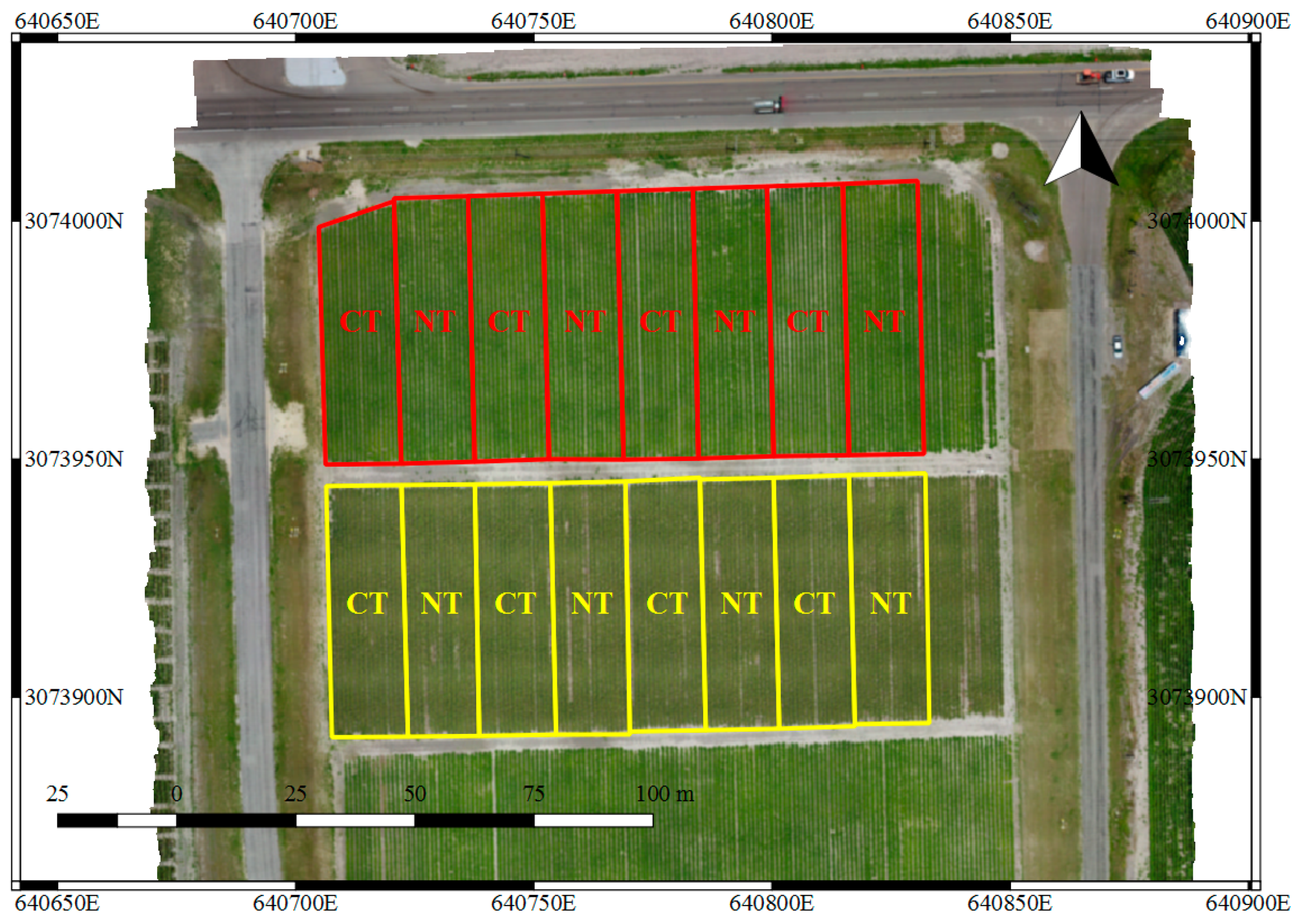
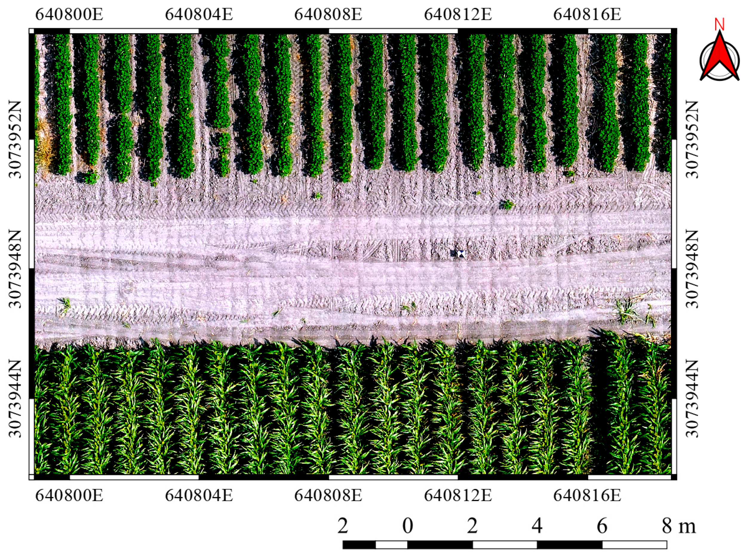
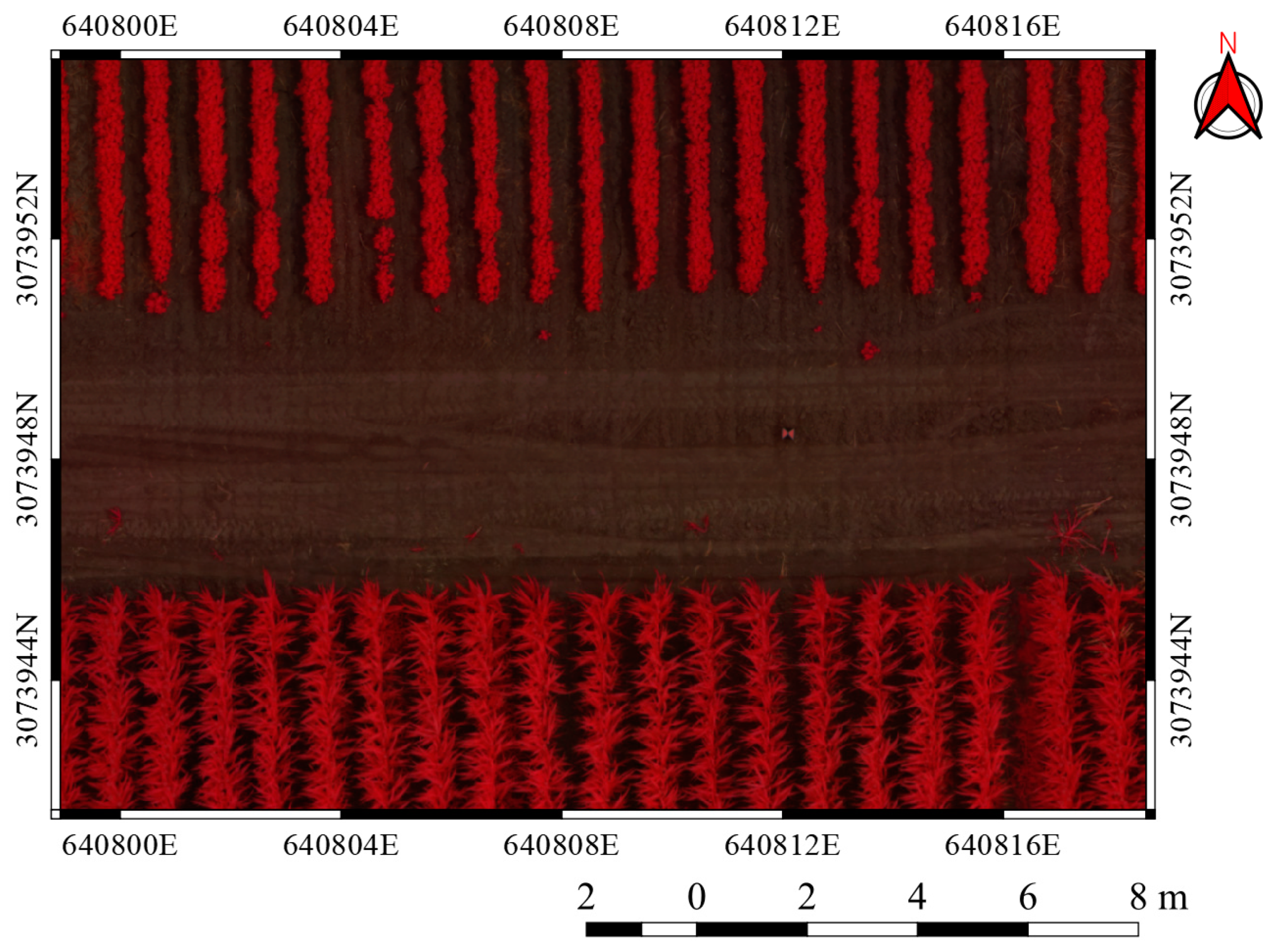
2. Study Area and Data

This study was conducted at the Texas A&M AgriLife Research and Extension Center at Corpus Christi, Texas, USA. The coordinates of the center of the field are approximately 27°46ʹ58.61ʺN latitude and 97°33ʹ43.95ʺW longitude. Soil types in the study site are Victoria Clay series soils (Victoria-Lattas-Clareville). Cotton and sorghum plots were established in a split plot design with CT and NT (Figure 1). Three cotton varieties (Deltapine, 1044, and B2RF) were planted on 25 March 2017 and harvested on 1 August. Three sorghum varieties (Dekalb, DKS, and 53-67) were planted on 19 March 2017 and harvested on 6 July and 11 July. Two rows by entire length (55 m each) per plot were mechanically harvested for cotton yield. Two sub-samples (4.2 m each) per plot were hand harvested for sorghum yield. The DJI Phantom 4 Pro platform and its 20 megapixels standard integrated sensor were used for RGB image acquisition. Another platform, DJI Matrice 100 with the SlantRange 3p sensor, was used to collect MS images. The SlantRange 3p sensor has a 1.2-megapixel resolution with a global shutter and captures NIR, red-edge, red, and green bands. Data collection timeline and flight conditions of each UAV platform are summarized in

Table 1. UAV data collection timeline and flight conditions.

Type	Date	Altitude	Overlap	Spatial Resolution (cm)
RGB	20 May 2017	30 m	80%	0.84
	30 May 2017	30 m	80%	0.76
	7 June 2017	30 m	80%	0.80
	14 June 2017	30 m	80%	0.79
	19 June 2017	30 m	80%	0.78
	5 July 2017	20 m	80%	0.51
	10 July 2017	30 m	80%	0.83
	18 July 2017	30 m	80%	0.82
	23 July 2017	25 m	85%	0.62
	1 August 2017	25 m	85%	0.68
NIR	20 May 2017	40 m	60%	1.69
	30 May 2017	40 m	60%	1.58
	7 June 2017	40 m	60%	1.58
	14 June 2017	40 m	60%	1.65
	19 June 2017	40 m	60%	1.62
	5 July 2017	40 m	60%	1.60
	10 July 2017	40 m	60%	1.64
	18 July 2017	40 m	60%	1.63
	23 July 2017	40 m	60%	1.67
	1 August 2017	40 m	75%	1.63

. Since sorghum was harvested earlier, only cotton remained on the last two collection dates.

Cotton (north) and sorghum (south) fields had eight plots each, composed of four CT and four NT treatments in a non-irrigated field, as shown in Figure 1. Each plot was approximately 900 m² and contained 16 rows (55 m long and 1 m apart). We generated 1 m²-sized grids in order to calculate plant-level VIs, and the number of grids was approximately 860 grids per plot. When we calculated VIs, a whole grid area (1 m²) that may include soil was used to consider crop abundance and vitality together (i.e., area weighted). If the canopy-covered area was clipped for VIs’ calculation, the difference between dense and sparse canopy grids would not be meaningful, e.g., a 10% covered grid with 0.7 average VIs versus a 100% covered grid with 0.6 average VIs. GPS surveying using ten ground control points (GCPs) evenly distributed on the entire study field was conducted for accurate geo-referencing. Subsequently, structure from motion (SfM) using Agisoft Photoscan Pro software was performed to generate RGB and MS orthomosaic images.

3. Methods

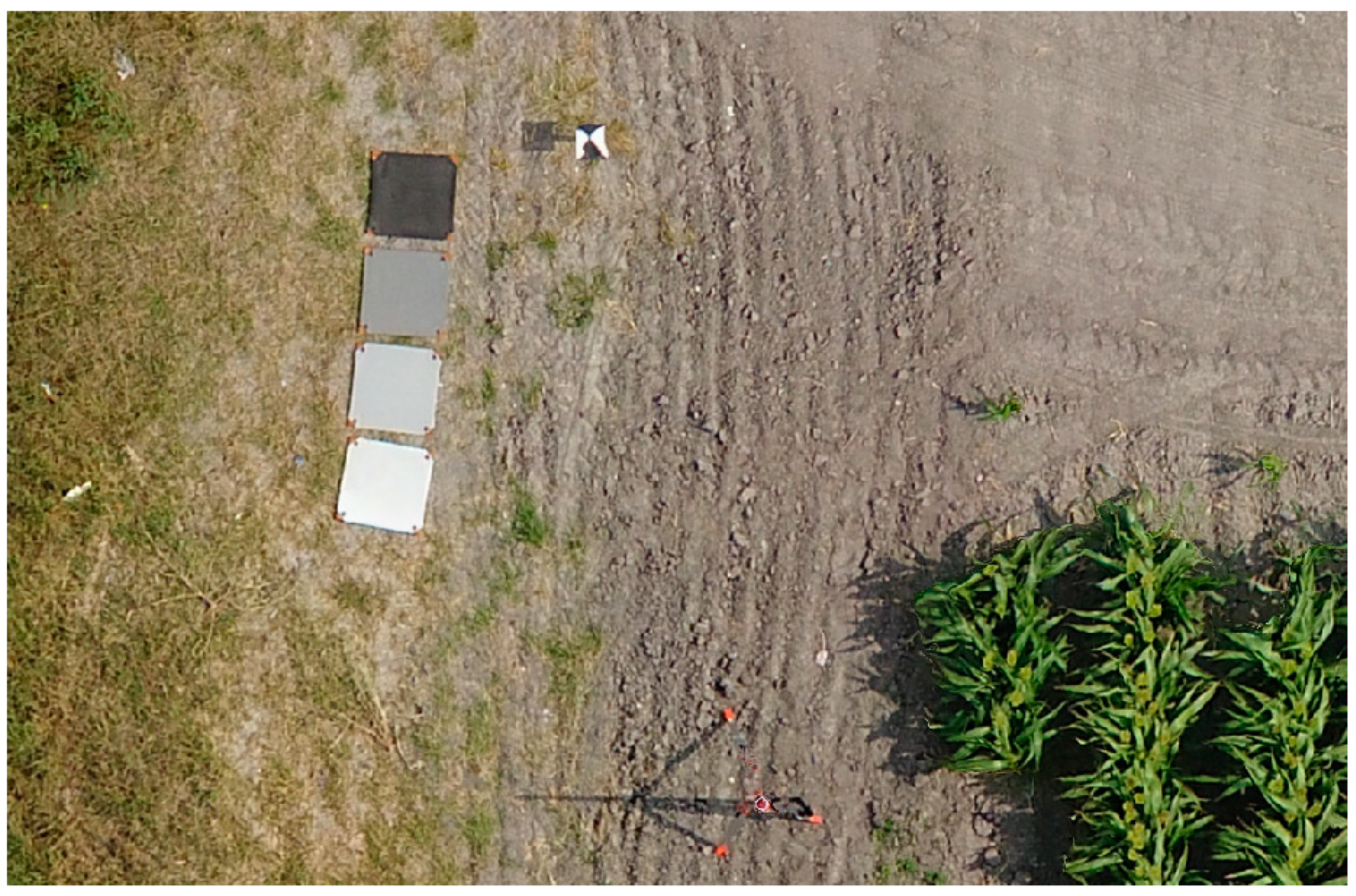
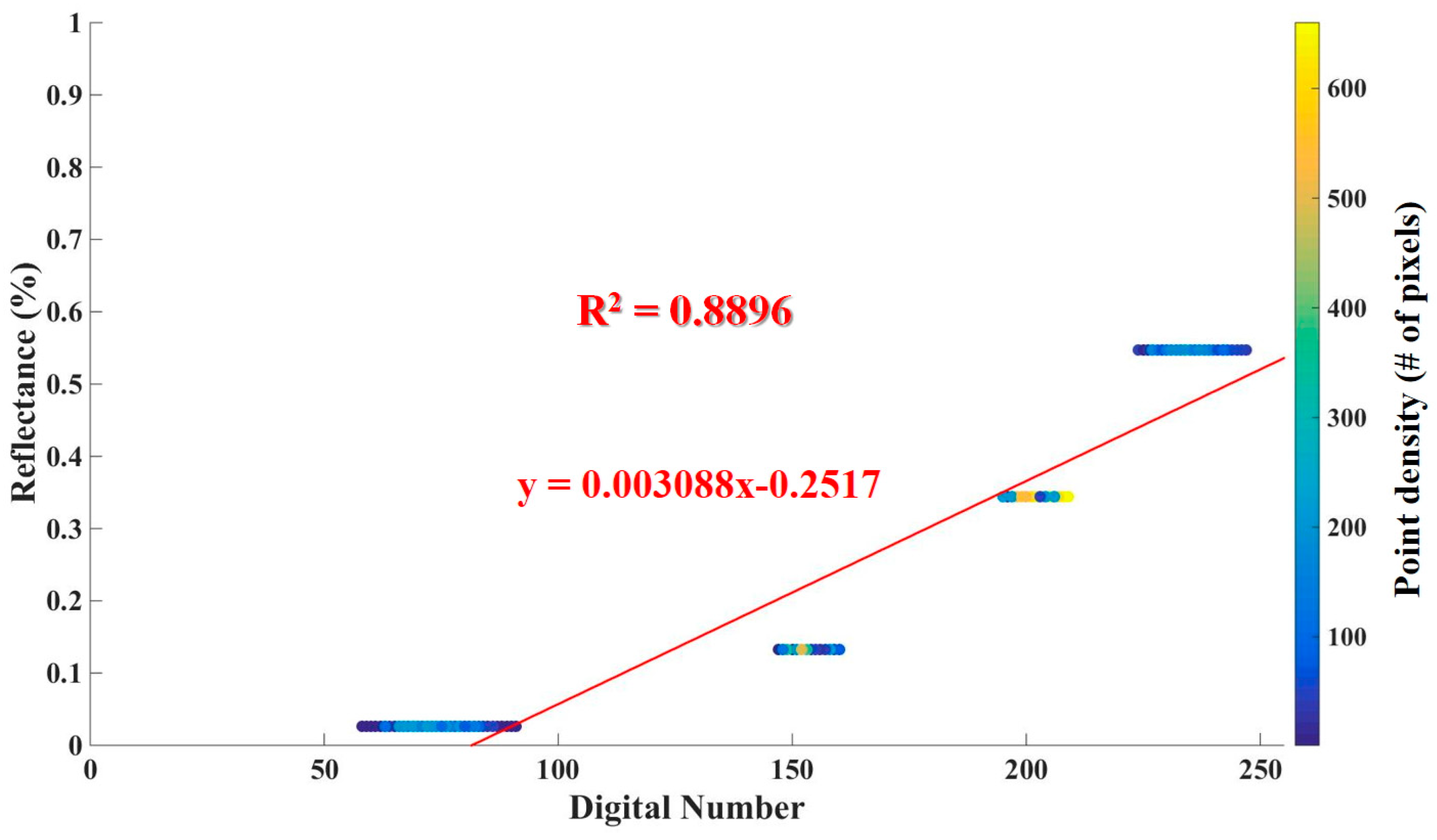
3.1. Radiometric Calibration

Digital numbers in UAV raw images should be radiometrically calibrated into reflectance values to calculate VIs. Radiometric calibration plays an important role especially when comparing VIs with multi-temporal data acquisitions since image digital numbers fluctuate depending on weather and illumination conditions. For radiometric calibration, two different methods were used depending on sensor types, RGB and multispectral (MS). Recent MS UAV platforms designed for agriculture applications basically are equipped with a sensor for illumination data collection or can be radiometrically calibrated by utilizing compatible reflectance panels. In the case of the SlantRange 3p MS sensor, it is equipped with an illumination sensor, and the ambient illumination sensor measures incident light conditions changing due to weather and the angle of the Sun. The illumination sensor is synchronized with MS camera exposure, and it enables frame-by-frame characterization of the solar irradiance. Therefore, crop conditions can be accurately compared across datasets gathered in all lighting conditions throughout the day and growing season. In this study, SlantView software for the processing of SlantRange data was used to perform radiometric calibration of raw images.

On the other hand, most of consumer-grade UAVs generally are equipped with only an RGB camera and do not have specific calibration systems. Therefore, in this study, reflectance panels having four different reflectivities were installed in the field whenever the data were collected and their known reflectance values in a specific wavelength were used as reference data for radiometric calibration. Pixels located within reflectance panels were manually clipped, and then, their digital numbers were compared with the actual reflectance values of the panels. The radiometric calibration was performed based on each date and each band. Linear calibration models between the digital numbers of the clipped pixels and the corresponding ground reflectance values of the panels were generated using Equation (1):

$$\begin{array}{c}{r}_i^c={\widehat{\beta }}_0^c+{\widehat{\beta }}_1^c{d}_i^c,\\ S{S}_{dr}^c={\displaystyle \sum }{d}_i^c{r}_i^c-\frac{\left({\displaystyle \sum }{d}_i^c\right)\left({\displaystyle \sum }{r}_i^c\right)}{n^c},\\ S{S}_{dd}^c={\displaystyle \sum }{\left(d_i^c\right)}^2-\frac{{\left({\displaystyle \sum }{d}_i^c\right)}^2}{n^c},\\ {\widehat{\beta }}_1^c=\frac{S{S}_{dr}^c}{S{S}_{dd}^c},{\widehat{\beta }}_0^c={\overline{r}}^c-{\widehat{\beta }}_1^c{\overline{d}}^c,\end{array}$$

(1)

where superscript $c$ denotes calibration cases for each acquisition date and spectral band, $r_i$ and $d_i$ are the reflectance value and the digital number of the $i$^th pixel, ${\widehat{\beta }}_0$ and ${\widehat{\beta }}_1$ are the estimated values of the y-intercept and slope in a linear calibration model, $S{S}_{dr}$ and $S{S}_{dd}$ are the sum of squares for digital number-reflectance value pairs and digital numbers, respectively, $n$ is the total number of pixels, and $\overline{r}$ and $\overline{d}$ are the average values of reflectance values and digital numbers. From the estimated y-intercept (${\widehat{\beta }}_0$) and slope (${\widehat{\beta }}_1$) parameters in each linear model, all pixels in the corresponding RGB UAV image were calibrated into reflectance values.

3.2. RGB and NIR VIs

Since NDVI was introduced in 1970s, many VIs have been developed using new sensors and spectral bands for diverse research topics. VIs have their own specialties with regard to soil brightness adjustment, water amount, crop stress, crop chlorophyll, etc. In this study, we adopted five RGB VIs [32,33] and eight red edge- or NIR-related VIs, referred to as “NIR VIs” [34,35], that showed superiority for agricultural analysis in the previous comparison studies. As of now, few NIR VIs comparison studies using UAV data have been explored for agriculture analysis. Therefore, in this study, pioneering research for the application of NIR VIs to UAV data was considered and evaluated. The VIs used in this study are summarized in Table 2:

Table 2. Vegetation indices used in this study.

Type	Name	Equation	Reference
RGB	GRVI (green red vegetation index)	$\frac{G-R}{G+R}$	[36]
	MGRVI (modified green red vegetation index)	$\frac{G^2-R^2}{G^2+R^2}$	[33]
	RGBVI (red green blue vegetation index)	$\frac{G^2-R\times B}{G^2+R\times B}$	[33]
	ExG (excess green)	2$G_{\mathrm{n}}-R_{\mathrm{n}}-B_{\mathrm{n}}$	[37]
	ExGR (excess green minus excess red)	$ExG-1.4R_{\mathrm{n}}-G_{\mathrm{n}}$	[38]
NIR	NDVI (normalized difference vegetation index)	$\frac{N-R}{N+R}$	[39]
	NDRE (normalized difference red edge index)	$\frac{N-E}{N+E}$	[40]
	GNDVI (green normalized difference vegetation index)	$\frac{N-G}{N+G}$	[41]
	SAVI (soil adjusted vegetation index)	$\frac{\left(N-R\right)\left(1+\alpha \right)}{N+R+\alpha }, \alpha =0.5$	[42]
	OSAVI (optimized soil adjusted vegetation index)	$\frac{\left(N-R\right)\left(1+\alpha \right)}{N+R+\alpha }, \alpha =0.16$	[43]
	MSAVI (modified soil adjusted vegetation index)	$\frac{2N+1-\sqrt{{\left(2N+1\right)}^2-8\left(N-R\right) }}{2}$	[44]
	GCI (green chlorophyll index)	$\frac{N}{G}-1$	[41]
	RECI (red edge chlorophyll index)	$\frac{N}{E}-1$	[41]

Table 2. Vegetation indices used in this study.

Type	Name	Equation	Reference
RGB	GRVI (green red vegetation index)	$\frac{G-R}{G+R}$	[36]
	MGRVI (modified green red vegetation index)	$\frac{G^2-R^2}{G^2+R^2}$	[33]
	RGBVI (red green blue vegetation index)	$\frac{G^2-R\times B}{G^2+R\times B}$	[33]
	ExG (excess green)	2$G_{\mathrm{n}}-R_{\mathrm{n}}-B_{\mathrm{n}}$	[37]
	ExGR (excess green minus excess red)	$ExG-1.4R_{\mathrm{n}}-G_{\mathrm{n}}$	[38]
NIR	NDVI (normalized difference vegetation index)	$\frac{N-R}{N+R}$	[39]
	NDRE (normalized difference red edge index)	$\frac{N-E}{N+E}$	[40]
	GNDVI (green normalized difference vegetation index)	$\frac{N-G}{N+G}$	[41]
	SAVI (soil adjusted vegetation index)	$\frac{\left(N-R\right)\left(1+\alpha \right)}{N+R+\alpha }, \alpha =0.5$	[42]
	OSAVI (optimized soil adjusted vegetation index)	$\frac{\left(N-R\right)\left(1+\alpha \right)}{N+R+\alpha }, \alpha =0.16$	[43]
	MSAVI (modified soil adjusted vegetation index)	$\frac{2N+1-\sqrt{{\left(2N+1\right)}^2-8\left(N-R\right) }}{2}$	[44]
	GCI (green chlorophyll index)	$\frac{N}{G}-1$	[41]
	RECI (red edge chlorophyll index)	$\frac{N}{E}-1$	[41]

where $N$, $E$, $R$, $G$, and $B$ denote NIR, red-edge, red, green, and blue bands, respectively. $R_{\mathrm{n}}$, $G_{\mathrm{n}}$, and $B_{\mathrm{n}}$ indicate normalized red, green, and blue images, respectively, and they are derived by Equation (2):

$$\begin{array}{c}{R}_{\mathrm{n}}=\frac{R}{R+G+B},\\ G_{\mathrm{n}}=\frac{G}{R+G+B},\\ B_{\mathrm{n}}=\frac{B}{R+G+B}.\end{array}$$

(2)

3.3. Time Series Difference Analysis and Z-Test

UAV data collection was conducted on a weekly basis over the study area to monitor crop growth. The images of time series VIs were clipped based on small GIS grids (1 m by 1 m) since row spacing in the field was 1 m, such that plant-level VIs were acquired. The average values of VIs within each grid were calculated, and then, the average values of the grids within each plot were summarized based on tillage treatment and crop type. Temporal variations of VIs in CT and NT fields were plotted in the time domain and compared with each other to analyze the difference resulting from the tillage treatments. The multi-temporal differences of VIs between CT and NT fields were quantitatively measured using the normalized root mean squared deviation (NRMSD), as in Equation (3):

$$\mathrm{NRMSD}(\%)=\sqrt{\frac{{{\displaystyle \sum }}_{i=1}^n{\left(V{I}_i^{\mathrm{c}}-V{I}_i^{\mathrm{n}}\right)}^2}{n}}/\left(\max \left(V{I}^{\mathrm{c}},V{I}^{\mathrm{n}}\right)-\min \left(V{I}^{\mathrm{c}},V{I}^{\mathrm{n}}\right)\right)\times 100,$$

(3)

where $V{I}_i^{\mathrm{c}}$ and $V{I}_i^{\mathrm{n}}$ are the average values of VIs in $i$^th data acquisition date of the CT and NT fields, respectively, $n$ is the total number of data acquisition dates, and $\max \left(V{I}^{\mathrm{c}},V{I}^{\mathrm{n}}\right)$ and $\min \left(V{I}^{\mathrm{c}},V{I}^{\mathrm{n}}\right)$ are the maximum and minimum of average values in entire fields for all dates. As VIs have different ranges, they should be normalized using the range between maximum and minimum values before the comparison, as in Equation (3).

In addition, a one-tailed Z-test for time series data was conducted for statistical verification of VIs’ difference between CT and NT fields. The average and variance of VIs on plant-level grids for each tillage treatment were calculated. RGB and NIR VIs on each date were evaluated using a 0.05 significance level ($\alpha$) to compare VIs in terms of tillage effect differentiation. The null and alternate hypotheses of the Z-test were set as follows: ${\mathrm{H}}_0$ (null hypothesis): the VIs in NT are not significantly greater than CT; ${\mathrm{H}}_1$ (alternate hypothesis): the VIs in NT are significantly greater than CT. When the Z statistic in Equation (4) is larger than 1.645, the null hypothesis would be rejected, which indicates significant VI difference between CT and NT fields at the 0.05 significance level.

$$\mathrm{Z}=\frac{{\mu }_i^{\mathrm{n}}-{\mu }_i^{\mathrm{c}}}{\sqrt{\frac{{\left({\sigma }_i^{\mathrm{n}}\right)}^2}{n}+\frac{{\left({\sigma }_i^{\mathrm{c}}\right)}^2}{n}}},$$

(4)

where ${\mu }_i^{\mathrm{n}}$ and ${\mu }_i^{\mathrm{c}}$ represent the average NT and CT VIs for data acquisition date i, respectively. ${\sigma }_i^{\mathrm{n}}$ and ${\sigma }_i^{\mathrm{c}}$ represent the standard deviation of NT and CT VIs for data acquisition date $i$, respectively. $n$ means the number of grids.

4. Results and Discussion

4.1. Radiometric Calibration

The pixels located within the boundaries of reflectance panels, approximately 2850 pixels per panel on each date, were collected for the radiometric calibration of RGB orthomosaic images (Figure 2). The pixels near panel boundaries were avoided to ensure selected pixels correctly represented actual reflectance values. As panels had different reflectance values depending on spectral wavelengths as described in

Table 3. Reflectance values of reference panels.

Reflectance (%)		Wavelength (nm)
		460 nm (Blue)	525 nm (Green)	625 nm (Red)
Reflectance panels	Black	2.5694	2.5794	2.6259
	Dark gray	13.2275	13.0259	12.7661
	Light gray	34.3803	33.9623	33.3508
	White	54.7198	55.6298	56.1708

, linear calibration models were generated using actual reflectance values of each panel in each wavelength and digital numbers of orthomosaic images in corresponding band. Figure 3 shows one of the generated radiometric calibration models. It can be observed from Figure 3 that the pixels with digital numbers lower than the x-intercept value would have a zero reflectance value. Calibration parameters, slope, and y-intercept varied according to the input images as the weather and illumination conditions were different. Therefore, the radiometric calibration was performed based on each date and each band. The general range of calibrated reflectance values was from 0–0.7. Figure 4 shows the calibrated RGB orthomosaic image acquired on 20 May.

In the case of RGB images, radiometric calibration using reflectance panels was required because the RGB platform was basically designed for cost-efficient operation without calibration systems. Conversely, MS platforms are more expensive and are generally equipped with a calibration system. In the case of the SlantRange 3p MS sensor, it used the information acquired by an ambient illumination sensor, and radiometric calibration was conducted using SlantView software. The calibration result of the MS image acquired on 20 May with false color composition is shown in Figure 5.

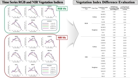
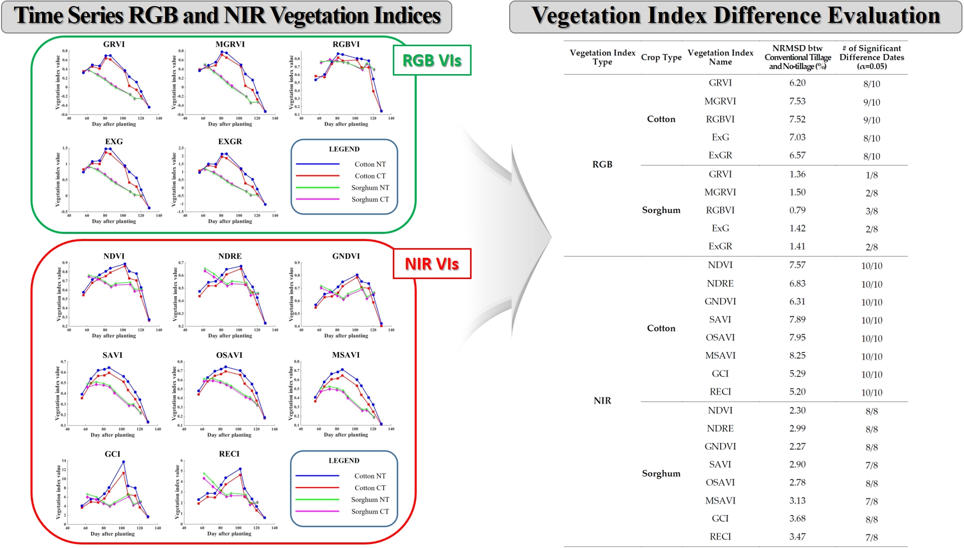
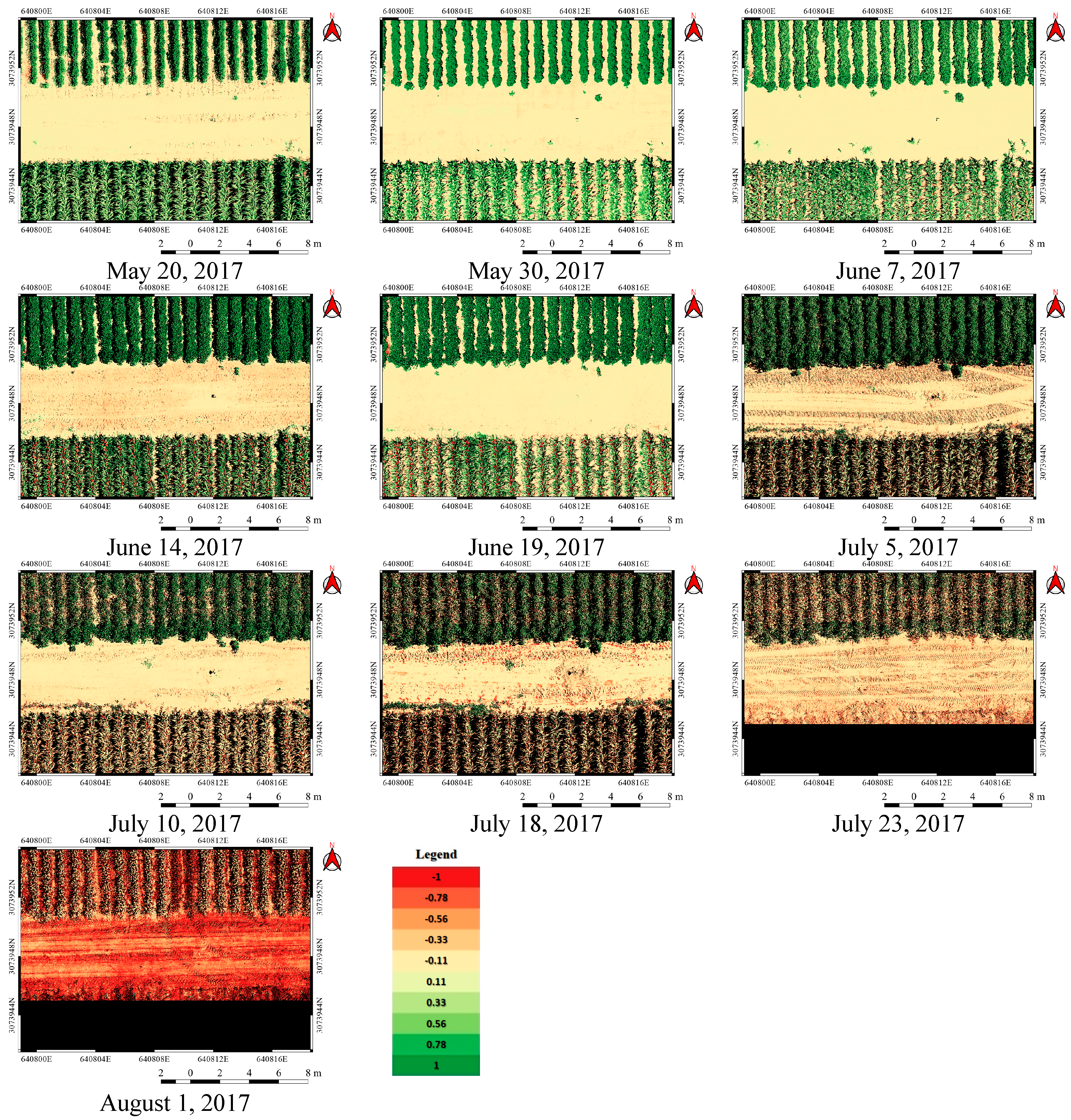
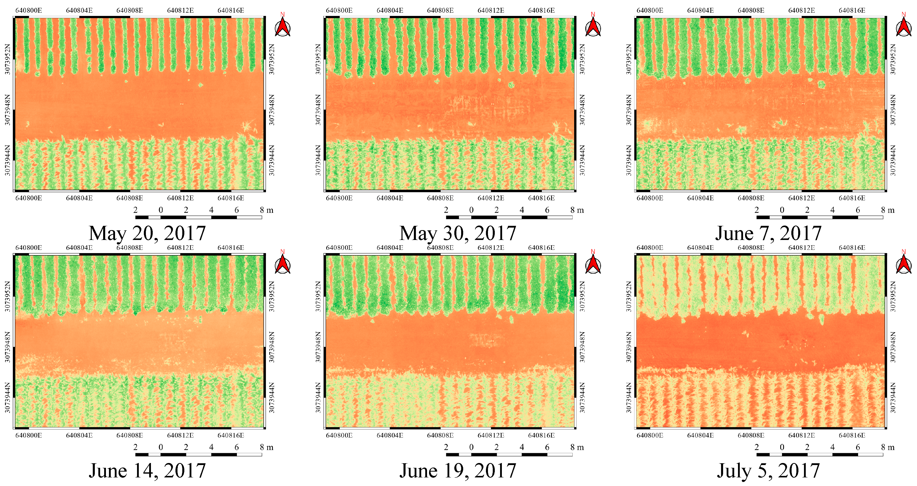
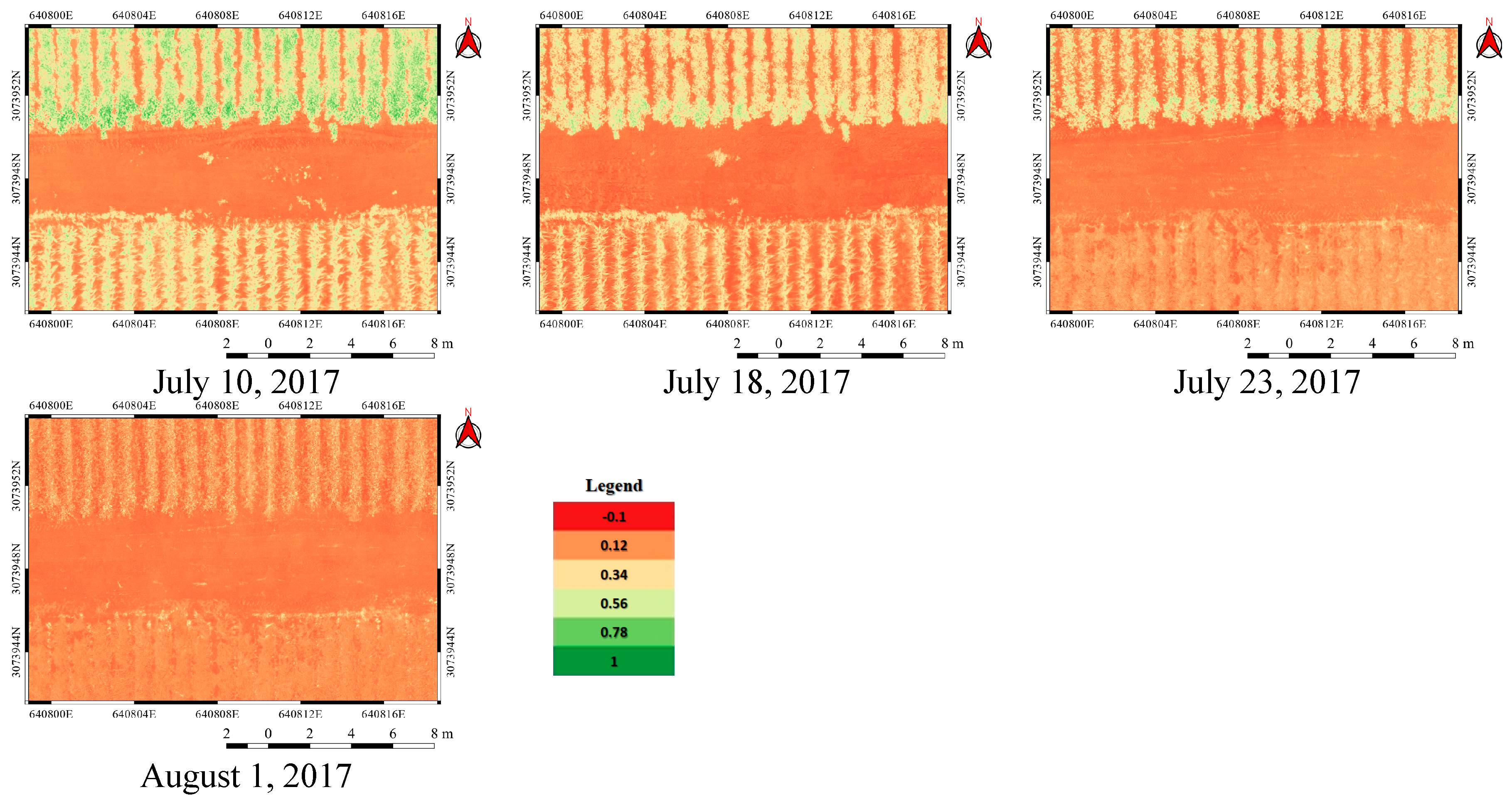
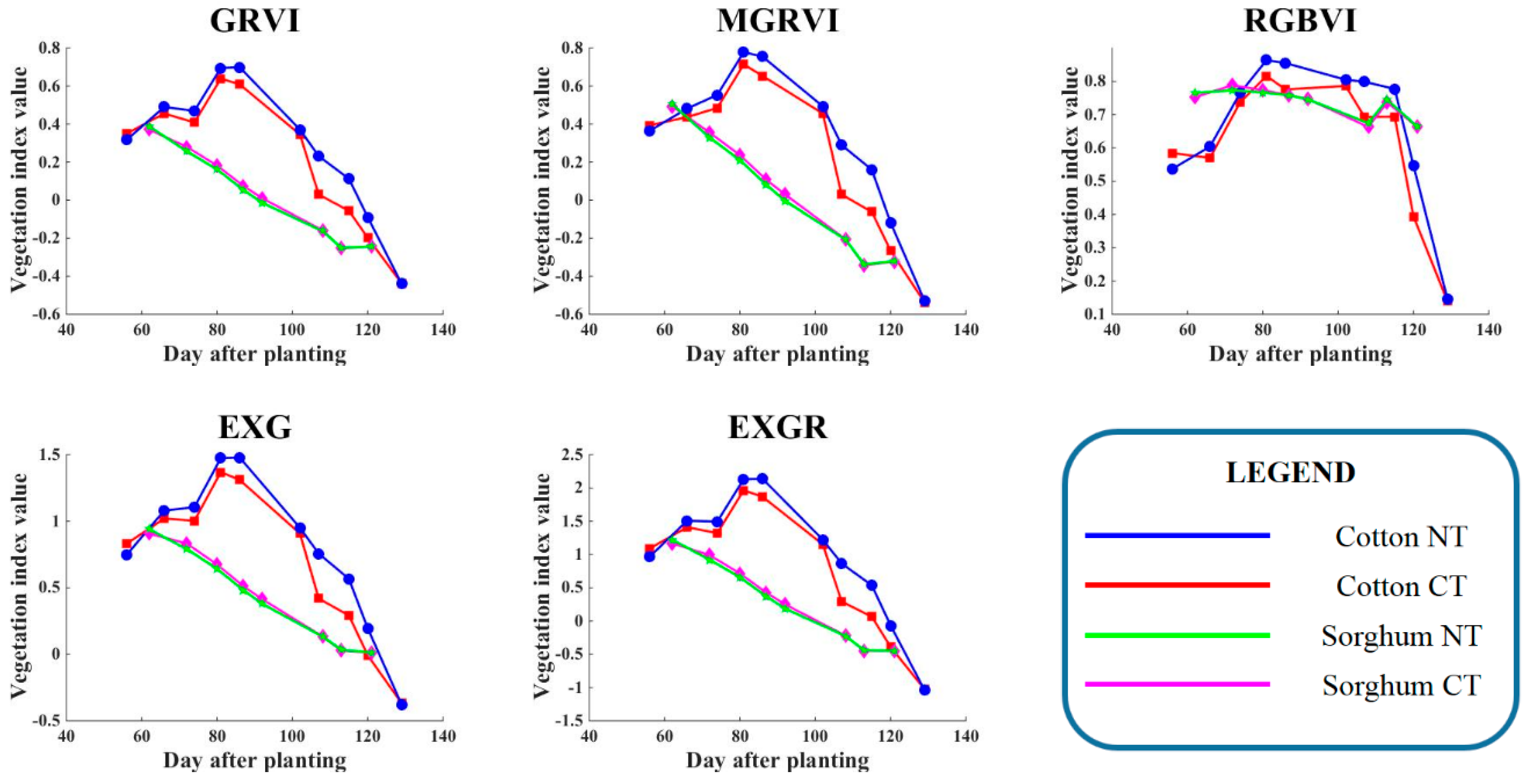
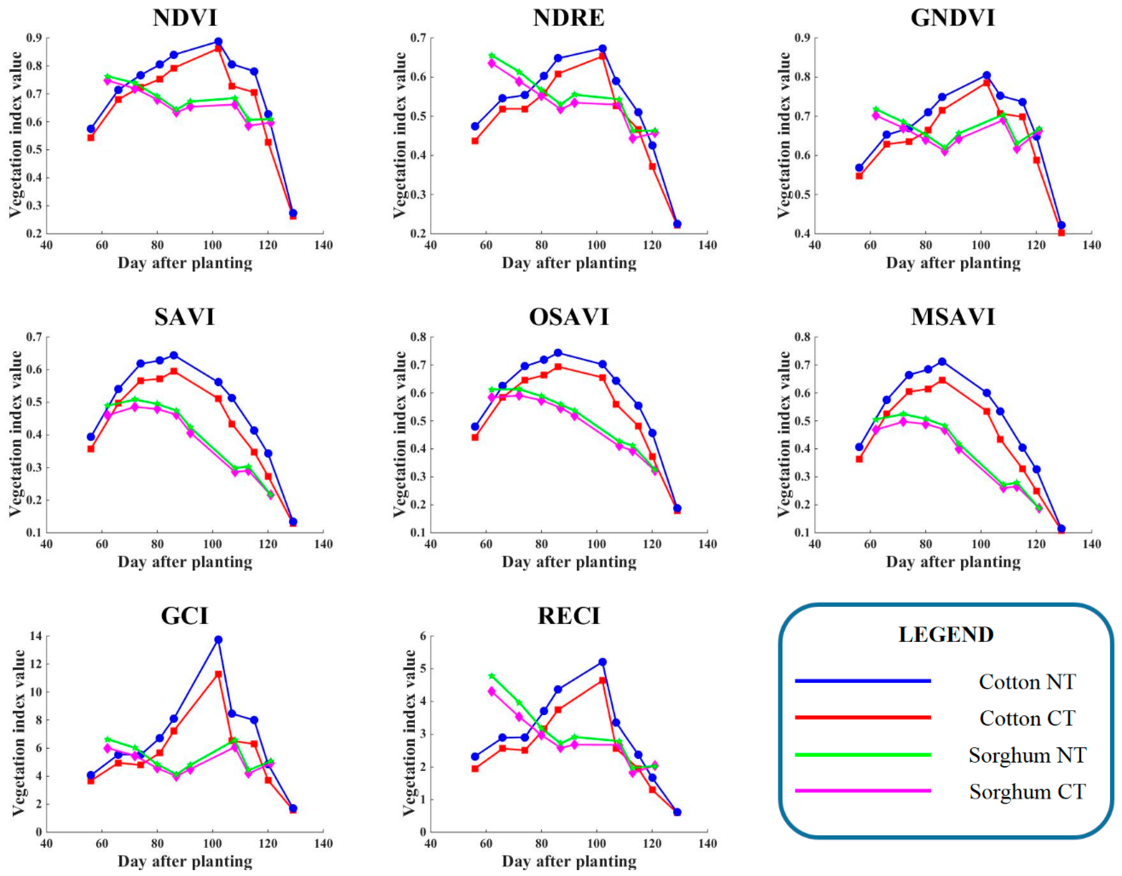
4.2. Time Series RGB and NIR VIs

Time series images of one RGB (MGRVI) and one NIR (MSAVI) VIs are shown in Figure 6 and Figure 7, respectively. We selected these two time series VIs for visualization because they finally showed better results in Section 4.3 among RGB and NIR VIs, respectively. It can be observed from Figure 6 that MGRVI in the cotton field (upper part in the images) maintained high values until 5 July (102 days after planting) and then started to decrease. As the sorghum field matured earlier than the cotton field, MGRVI in the sorghum field (lower part in the images) started to decrease after 19 June (92 days after planting), earlier than the cotton field. When shadows were present in RGB orthomosaic images, calibrated RGB reflectance values of the shadows were very low, which made some RGB VIs have “not a number” values since the denominator of the equation may be zero. For this reason, the linear calibration method using reflectance panels may have a problem with representing VIs of shadowed crops in RGB images. Therefore, we represented “not a number” values as black color in Figure 6 and excluded them from the calculation. MSAVI in the cotton field increased until mid-June (82 days after planting) and then started to decrease. In the case of the sorghum field, MSAVI started to decrease on 19 June (92 days after planting), in common with MGRVI. MSAVI showed more smoothed image as compared to MGRVI since most of the values ranged between zero and one, while MGRVI showed high contrast due to more negative and occluded pixels resulting from noises and shadows (Figure 8). Other differences between MGRVI and MSAVI images resulted from the difference in spatial resolutions: (1) the high resolution of MGRVI can contribute to better detection of cotton bolls and sorghum heads, but (2) MGRVI is more sensitive to leaf shadows and noises (Figure 8). In both MGRVI and MSAVI images, it was difficult to visually interpret the tillage treatment difference between CT and NT fields.

The averaged values of grid VIs based on each tillage treatment and crop type were used for time series analysis. Comparison of VIs between CT and NT fields were conducted using the summarized values on each date. The temporal change of all RGB and NIR VIs is shown in Figure 9 and Figure 10. It can be observed that there were distinct differences in VI values between CT and NT fields during the whole season for both crops, except for RGB VIs in the sorghum field. The NT fields displayed higher values in most VIs than those of CT fields, which means the NT fields had more vigorous and abundant crops than the CT field. All NIR VIs showed consistently higher values in NT fields than CT fields throughout the season. As we assumed NT treatments can contribute to higher yield than CT [22], these results scientifically support the research hypothesis. The actual harvest yields of cotton and sorghum in NT fields were higher than CT fields. Cotton lint yield in NT fields was 17% higher than CT fields (367 g/m² > 315 g/m²), and sorghum yield in NT fields was 15% higher than CT fields (590 g/m² > 514 g/m²).

There were several aspects for which NIR VIs were superior to RGB VIs. First, the differences of NIR VIs between CT and NT fields were more consistent throughout the season. Second, NIR VIs detected the tillage treatment difference in the sorghum field, which was not possible from the RGB VIs. Third, NIR VIs generally fluctuated less than RGB VIs except for chlorophyll-related VIs (GCI and ECI). Especially soil adjusted NIR VIs (SAVI, OSAVI, and MSAVI) showed the most stable increase and decrease of VIs throughout the season, while they had a distinct difference between tillage treatments in both crop fields.

4.3. Difference Measurement and Evaluation

Differences of VIs between CT and NT fields were quantitatively measured using NRMSD and summarized in

Table 4. VIs’ difference measurement.

VIs Type	Crop Type	VIs Name	Peak Day after Plating (Days)	NRMSD between CT and NT (%)	# of Inflection Points
RGB	Cotton	GRVI	81(CT), 86(NT)	6.20	3
		MGRVI	81	7.53	1
		RGBVI	81	7.52	6(CT), 1(NT)
		ExG	81(CT), 86(NT)	7.03	3(CT), 1(NT)
		ExGR	81(CT), 86(NT)	6.57	3
	Sorghum	GRVI	-	1.36	1
		MGRVI	-	1.50	1
		RGBVI	-	0.79	3
		ExG	-	1.42	0
		ExGR	-	1.41	1(CT), 0(NT)
NIR	Cotton	NDVI	102	7.57	1
		NDRE	102	6.83	3(CT), 1(NT)
		GNDVI	102	6.31	1
		SAVI	86	7.89	1
		OSAVI	86	7.95	1
		MSAVI	86	8.25	1
		GCI	102	5.29	3
		RECI	102	5.20	3(CT), 1(NT)
	Sorghum	NDVI	-	2.30	3
		NDRE	-	2.99	3(CT), 2(NT)
		GNDVI	-	2.27	3
		SAVI	-	2.90	3
		OSAVI	-	2.78	1
		MSAVI	-	3.13	3
		GCI	-	3.68	3
		RECI	-	3.47	3

with other factors. The number of inflection points indicates the amount of fluctuation in VIs and includes local minimum and maximum points. The fluctuation in time series data is regarded as noise, and the noise removal process is required for better metric estimation [45,46]. The peak point is supposed to be only one if the data collection period covers whole crop growth stages. In this study, the cotton and sorghum fields should have respectively one and zero peak points (one and zero inflection points accordingly) due to their crop development stages. The peak date of VIs in the cotton field varied between 81 and 102 days after planting depending on formulas and tillage treatments. Although NDVI is widely used in most crop research, the result confirmed that the performance of VIs varies depending on formulas and spectral band types. Especially, soil adjusted NIR VIs (SAVI, OSAVI, and MSAVI) outperformed NDVI in terms of NRMSD. In addition, as discussed in Section 4.2, soil adjusted NIR VIs showed the most stable increase and decrease compared to any other RGB VIs, simple ratio NIR VIs (NDVI, NDRE, and GNDVI), and chlorophyll-related VIs (GCI and RECI). The top 2 and 3 VIs having high NRMSD among RGB and NIR VIs, respectively, are highlighted in Table 4. It can be confirmed from Table 4 that the NIR VIs are better indicators for tillage effect analysis than RGB VIs because the NRMSDs of NIR VIs were remarkably higher than those of RGB VIs in the sorghum field. Average NRMSDs of NIR VIs in the cotton field (except GCI and RECI) were also higher than those of RGB VIs. We compared VIs between NT and CT for each date to check if the VIs in NT were higher than those of CT. As a result of the comparison, all NIR VIs had consistently higher VIs in NT fields for all the dates and for both crops, which was not the case of all RGB VIs. However, it is encouraging that some RGB VIs such as MGRVI and RGBVI showed a similar level of NRMSD as NIR VIs.

MGRVI had the highest NRMSDs of 7.53% and 1.50% among RGB VIs in the cotton and sorghum fields, respectively. The problem of other RGB VIs was that they had more inflection points than one in the cotton field. In the case of the sorghum field, ExG showed similar NRMSD to MGRVI and a more exact number of inflection points. Among NIR VIs, MSAVI showed the highest NRMSD of 8.25% and one inflection point in the cotton field. On the sorghum field, OSAVI showed high NRMSD with a lower number of inflection points. Although NRMSDs of chlorophyll-related VIs (GCI and RECI) were higher than soil adjusted VIs (SAVI, OSAVI, and MSAVI) in the sorghum field, the fluctuation of VIs in both crop fields and low NRMSD in the cotton field could be problems.

A one-tailed Z-test using time series data was performed for statistical verification of the difference in VIs between CT and NT fields. The null hypothesis of the Z-test was set as the VIs in NT were not significantly greater than CT, and it would be rejected when Z statistic was larger than 1.645 at the significance level of 0.05. The time series Z-test results are summarized in

Table 5. Time series Z-test results between CT and NT fields.

VIs Type	Crop Type	VIs Name	Dates										# of Significant Dates (α = 0.05)
			20 May	30 May	7 June	14 June	19 July	5 July	10 July	18 July	23 July	1 August
RGB	Cotton	GRVI	−14.76	19.34	32.68	27.18	35.59	13.28	45.69	44.07	33.99	−1.29	8/10
		MGRVI	−10.86	21.29	32.45	31.88	38.52	15.92	46.40	44.75	34.77	4.20	9/10
		RGBVI	−20.77	20.21	16.39	34.13	45.11	18.69	50.82	48.01	46.74	2.80	9/10
		ExG	−20.91	19.22	31.15	29.85	38.30	13.54	47.69	45.46	37.04	−5.31	8/10
		ExGR	−19.17	19.22	32.15	28.32	36.99	12.98	46.55	44.56	35.39	−3.21	8/10
	Sorghum	GRVI	4.87	−7.98	−10.59	−11.16	−17.61	−2.06	1.11	−0.04	-	-	1/8
		MGRVI	2.61	−6.76	−9.74	−10.28	−17.82	−0.52	1.95	0.75	-	-	2/8
		RGBVI	3.54	−3.83	−2.01	0.02	−0.29	3.75	3.03	0.62	-	-	3/8
		ExG	5.22	−7.59	−8.30	−8.38	−12.94	−0.23	2.68	0.39	-	-	2/8
		ExGR	5.17	−7.92	−9.47	−9.89	−15.53	−1.04	1.85	0.12	-	-	2/8
NIR	Cotton	NDVI	21.38	27.26	37.31	40.67	42.57	29.69	48.44	45.83	47.92	19.25	10/10
		NDRE	28.80	25.47	31.56	30.61	34.01	22.58	47.21	35.30	40.98	9.04	10/10
		GNDVI	21.31	25.35	37.46	40.47	35.64	24.59	42.31	35.11	45.40	23.64	10/10
		SAVI	32.57	34.43	39.21	42.52	37.61	31.08	48.68	38.75	44.41	12.38	10/10
		OSAVI	29.86	32.98	39.62	44.72	40.93	34.17	50.80	43.22	46.64	15.98	10/10
		MSAVI	33.26	35.82	41.50	43.22	39.73	30.62	48.08	37.39	42.92	11.02	10/10
		GCI	23.51	26.06	33.52	33.11	25.26	28.46	40.11	30.23	38.39	21.38	10/10
		RECI	31.57	27.61	29.48	24.85	29.43	21.05	46.30	31.78	37.34	8.79	10/10
	Sorghum	NDVI	6.14	8.41	5.28	5.33	9.92	14.37	15.70	8.02	-	-	8/8
		NDRE	10.00	14.30	9.31	8.79	15.35	13.24	21.05	4.86	-	-	8/8
		GNDVI	9.25	9.06	7.42	5.88	9.67	9.83	11.77	3.65	-	-	8/8
		SAVI	16.08	11.82	8.84	8.29	11.77	11.39	14.72	1.05	-	-	7/8
		OSAVI	13.42	10.79	7.52	7.05	11.40	14.42	17.44	3.89	-	-	8/8
		MSAVI	17.12	12.06	9.07	8.35	12.21	10.74	13.96	0.12	-	-	7/8
		GCI	16.57	16.94	10.65	6.12	12.90	12.09	10.61	5.98	-	-	8/8
		RECI	15.26	18.51	11.35	9.98	17.03	8.61	17.73	−0.90	-	-	7/8

, and significant dates are underlined and counted. All NIR VIs showed high Z statistics and significant differences between CT and NT fields for all data except SAVI, MSAVI, and RECI on the last date in the sorghum field. NIR VIs had higher Z statistics than RGB VIs, and the number of significant dates of NIR VIs was more than RGB VIs for both crops. In the case of RGB VIs for the cotton field, the number of significant dates was 8~9 out of 10 dates, which was less than those of NIR VIs (10 significant dates for all VIs). Especially in the case of RGB VIs for the sorghum field, only 1~3 dates were significant. Conversely, NIR VIs in the sorghum field had good significance, which was 7~8 dates out of eight dates. Considering analysis of time series graphs, quantitative difference measurements using NRMSD, and Z-test results, we concluded that MGRVI and ExG among RGB VIs and MSAVI and OSAVI among NIR VIs were better VIs for differentiation of tillage practices.

5. Conclusions

In this study, various RGB and NIR VIs were applied to high-resolution multi-temporal UAV data for the analysis of tillage effects. The results confirmed that distinct differences in VIs existed between CT and NT fields during the whole growth period for cotton and sorghum. NT fields consistently displayed higher values in most VIs than CT fields. The difference between CT and NT treatments was quantitatively measured and statistically compared to support scientifically the research hypothesis that NT fields have more vigorous and abundant crops than CT fields, which could contribute to higher yield.

There were several aspects in which NIR VIs were superior to RGB VIs. First, the differences of NIR VIs between CT and NT fields were more consistent throughout the season. Second, NIR VIs caught the tillage treatment difference in the sorghum field, which was not possible from the RGB VIs. Third, NIR VIs generally fluctuated less than RGB VIs. Fourth, NIR VIs had higher Z statistics than RGB VIs, and the number of significant dates of NIR VIs was more than RGB VIs for both crops. Among RGB VIs, MGRVI and ExG showed good performance. Especially MSAVI and OSAVI among NIR VIs showed better results than other VIs in terms of fluctuation in time series graphs, NRMSD between CT and NT fields, and time series Z-test for statistical verification. Although RGB VIs were not as good as NIR VIs, MGRVI and ExG showed potential, which can be used for economic UAV application in agriculture areas. As future work, we will apply the proposed scheme to find better VIs according to different crop pressures such as water stress, insects, and diseases.

References

1. Arvor, D.; Jonathan, M.; Meirelles, M.S.P.; Dubreuil, V.; Durieux, L. Classification of MODIS EVI time series for crop mapping in the state of Mato Grosso, Brazil. Int. J. Remote Sens. 2011, 32, 7847–7871. [Google Scholar] [CrossRef]
2. Li, Q.; Cao, X.; Jia, K.; Zhang, M.; Dong, Q. Crop type identification by integration of high-spatial resolution multispectral data with features extracted from coarse-resolution time-series vegetation index data. Int. J. Remote Sens. 2014, 35, 6076–6088. [Google Scholar] [CrossRef]
3. Sonobe, R.; Yamaya, Y.; Tani, H.; Wang, X.; Kobayashi, N.; Mochizuki, K.I. Crop classification from Sentinel-2-derived vegetation indices using ensemble learning. J. Appl. Remote Sens. 2018, 12, 026019. [Google Scholar] [CrossRef] [Green Version]
4. De Souza, C.H.W.; Mercante, E.; Johann, J.A.; Lamparelli, R.A.C.; Uribe-Opazo, M.A. Mapping and discrimination of soya bean and corn crops using spectro-temporal profiles of vegetation indices. Int. J. Remote Sens. 2015, 36, 1809–1824. [Google Scholar] [CrossRef]
5. Murakami, T.; Ogawa, S.; Ishitsuka, N.; Kumagai, K.; Saito, G. Crop discrimination with multitemporal SPOT/HRV data in the Saga plains, Japan. Int. J. Remote Sens. 2001, 22, 1335–1348. [Google Scholar] [CrossRef]
6. Siachalou, S.; Mallinis, G.; Tsakiri-Strati, M. Analysis of time-series spectral index data to enhance crop identification over a Mediterranean rural landscape. IEEE Geosci. Remote Sens. Lett. 2017, 14, 1508–1512. [Google Scholar] [CrossRef]
7. Yu, B.; Shang, S. Multi-year mapping of maize and sunflower in Hetao irrigation district of China with high spatial and temporal resolution vegetation index series. Remote Sens. 2017, 9, 855. [Google Scholar] [CrossRef]
8. Zheng, Y.; Zhang, M.; Zhang, X.; Zeng, H.; Wu, B. Mapping winter wheat biomass and yield using time series data blended from PROBA-V 100-and 300-m S1 products. Remote Sens. 2016, 8, 824. [Google Scholar] [CrossRef]
9. Gouveia, C.M.; Trigo, R.M.; Beguería, S.; Vicente-Serrano, S.M. Drought impacts on vegetation activity in the Mediterranean region: An assessment using remote sensing data and multi-scale drought indicators. Glob. Planet. Chang. 2017, 151, 15–27. [Google Scholar] [CrossRef]
10. Jay, S.; Maupas, F.; Bendoula, R.; Gorretta, N. Retrieving LAI, chlorophyll and nitrogen contents in sugar beet crops from multi-angular optical remote sensing: Comparison of vegetation indices and PROSAIL inversion for field phenotyping. Field Crop. Res. 2017, 210, 33–46. [Google Scholar] [CrossRef] [Green Version]
11. Kooistra, L.; Clevers, J.G.P.W. Estimating potato leaf chlorophyll content using ratio vegetation indices. Remote Sens. Lett. 2016, 7, 611–620. [Google Scholar] [CrossRef] [Green Version]
12. Serbin, G.; Hunt, E.R., Jr.; Daughtry, C.S.T.; McCarty, G.W. Assessment of spectral indices for cover estimation of senescent vegetation. Remote Sens. Lett. 2013, 4, 552–560. [Google Scholar] [CrossRef]
13. Sivanpillai, R.; Claypool, D.A.; Siloju, R. Relating AEROCam-derived NDVI to apparent soil electrical conductivity (ECa) for corn fields in Wyoming, USA. Remote Sens. Lett. 2012, 3, 49–56. [Google Scholar] [CrossRef]
14. Zhang, C.; Ren, H.; Qin, Q.; Ersoy, O.K. A new narrow band vegetation index for characterizing the degree of vegetation stress due to copper: The copper stress vegetation index (CSVI). Remote Sens. Lett. 2017, 8, 576–585. [Google Scholar] [CrossRef]
15. Bala, S.K.; Islam, A.S. Correlation between potato yield and MODIS-derived vegetation indices. Int. J. Remote Sens. 2009, 30, 2491–2507. [Google Scholar] [CrossRef]
16. Esquerdo, J.C.D.M.; Zullo Júnior, J.; Antunes, J.F.G. Use of NDVI/AVHRR time-series profiles for soybean crop monitoring in Brazil. Int. J. Remote Sens. 2011, 32, 3711–3727. [Google Scholar] [CrossRef]
17. Huang, J.; Wang, H.; Dai, Q.; Han, D. Analysis of NDVI data for crop identification and yield estimation. IEEE J. Sel. Top. Appl. Earth Observ. Remote Sens. 2014, 7, 4374–4384. [Google Scholar] [CrossRef]
18. Jiang, Z.; Chen, Z.; Chen, J.; Ren, J.; Li, Z.; Sun, L. The estimation of regional crop yield using ensemble-based four-dimensional variational data assimilation. Remote Sens. 2014, 6, 2664–2681. [Google Scholar] [CrossRef]
19. Kern, A.; Barcza, Z.; Marjanović, H.; Árendás, T.; Fodor, N.; Bónis, P.; Bognár, P.; Lichtenberger, J. Statistical modelling of crop yield in Central Europe using climate data and remote sensing vegetation indices. Agric. For. Meteorol. 2018, 260, 300–320. [Google Scholar] [CrossRef]
20. Meroni, M.; Fasbender, D.; Balaghi, R.; Dali, M.; Haffani, M.; Haythem, I.; Hooker, J.; Lahlou, M.; Lopez-Lozano, R.; Mahyou, H.; et al. Evaluating NDVI data continuity between SPOT-VEGETATION and PROBA-V missions for operational yield forecasting in North African countries. IEEE Trans. Geosci. Remote Sens. 2016, 54, 795–804. [Google Scholar] [CrossRef]
21. Rembold, F.; Atzberger, C.; Savin, I.; Rojas, O. Using low resolution satellite imagery for yield prediction and yield anomaly detection. Remote Sens. 2013, 5, 1704–1733. [Google Scholar] [CrossRef]
22. Garonna, I.; Fazey, I.; Brown, M.E.; Pettorelli, N. Rapid primary productivity changes in one of the last coastal rainforests: The case of Kahua, Solomon Islands. Environ. Conserv. 2009, 36, 253–260. [Google Scholar] [CrossRef]
23. Huete, A.; Didan, K.; Miura, T.; Rodriguez, E.P.; Gao, X.; Ferreira, L.G. Overview of the radiometric and biophysical performance of the MODIS vegetation indices. Remote Sens. Environ. 2002, 83, 195–213. [Google Scholar] [CrossRef]
24. Lee, S.J.; Cho, J.; Hong, S.; Ha, K.J.; Lee, H.; Lee, Y.W. On the relationships between satellite-based drought index and gross primary production in the North Korean croplands, 2000–2012. Remote Sens. Lett. 2016, 7, 790–799. [Google Scholar] [CrossRef]
25. Liu, W.T.; Kogan, F. Monitoring Brazilian soybean production using NOAA/AVHRR based vegetation condition indices. Int. J. Remote Sens. 2002, 23, 1161–1179. [Google Scholar] [CrossRef]
26. Zhang, S.; Liu, L. The potential of the MERIS terrestrial chlorophyll index for crop yield prediction. Remote Sens. Lett. 2014, 5, 733–742. [Google Scholar] [CrossRef]
27. Metternicht, G. Vegetation indices derived from high-resolution airborne videography for precision crop management. Int. J. Remote Sens. 2003, 24, 2855–2877. [Google Scholar] [CrossRef]
28. Rud, R.; Shoshany, M.; Alchanatis, V. Spectral indicators for salinity effects in crops: A comparison of a new green indigo ratio with existing indices. Remote Sens. Lett. 2011, 2, 289–298. [Google Scholar] [CrossRef]
29. Milas, A.S.; Vincent, R.K. Monitoring Landsat vegetation indices for different crop treatments and soil chemistry. Int. J. Remote Sens. 2017, 38, 141–160. [Google Scholar] [CrossRef]
30. Triplett, G.B.; Dick, W.A. No-tillage crop production: A revolution in agriculture! Agron. J. 2008, 100, S-153–S-165. [Google Scholar] [CrossRef]
31. Pittelkow, C.M.; Linquist, B.A.; Lundy, M.E.; Liang, X.; Van Groenigen, K.J.; Lee, J.; Van Gestel, N.; Six, J.; Venterea, R.T.; Van Kessel, C. When does no-till yield more? a global meta-analysis. Field Crop. Res. 2015, 183, 156–168. [Google Scholar] [CrossRef]
32. Torres-Sánchez, J.; Peña, J.M.; De Castro, A.I.; López-Granados, F. Multi-temporal mapping of the vegetation fraction in early-season wheat fields using images from UAV. Comput. Electron. Agric. 2014, 103, 104–113. [Google Scholar] [CrossRef]
33. Bendig, J.; Yu, K.; Aasen, H.; Bolten, A.; Bennertz, S.; Broscheit, J.; Gnyp, M.L.; Bareth, G. Combining UAV-based plant height from crop surface models, visible, and near infrared vegetation indices for biomass monitoring in barley. Int. J. Appl. Earth Obs. Geoinf. 2015, 39, 79–87. [Google Scholar] [CrossRef]
34. Hatfield, J.L.; Prueger, J.H. Value of using different vegetative indices to quantify agricultural crop characteristics at different growth stages under varying management practices. Remote Sens. 2010, 2, 562–578. [Google Scholar] [CrossRef]
35. Eitel, J.U.H.; Keefe, R.F.; Long, D.S.; Davis, A.S.; Vierling, L.A. Active ground optical remote sensing for improved monitoring of seedling stress in nurseries. Sensors 2010, 10, 2843–2850. [Google Scholar] [CrossRef] [PubMed]
36. Tucker, C.J. Red and photographic infrared linear combinations for monitoring vegetation. Remote Sens. Environ. 1979, 8, 127–150. [Google Scholar] [CrossRef] [Green Version]
37. Woebbecke, D.M.; Meyer, G.E.; Von Bargen, K.; Mortensen, D.A. Color indices for weed identification under various soil, residue, and lighting conditions. Trans. ASAE 1995, 38, 259–269. [Google Scholar] [CrossRef]
38. Camargo Neto, J. A Combined Statistical-Soft Computing Approach for Classification and Mapping Weed Species in Minimum-Tillage Systems. ETD Collection for University of Nebraska-Lincoln. Ph.D. Thesis, University of Nebraska-Lincoln, Lincoln, NE, USA, 2004. [Google Scholar]
39. Rouse, J.W., Jr.; Haas, R.H.; Schell, J.A.; Deering, D.W. Monitoring vegetation systems in the Great Plains with ERTS. In NASA Goddard Space Flight Center 3d ERTS-1 Symposium; NASA: Washington, DC, USA, 1974; Volume 1, pp. 309–317. [Google Scholar]
40. Barnes, E.M.; Clarke, T.R.; Richards, S.E.; Colaizzi, P.D.; Haberland, J.; Kostrzewski, M.; Waller, P.; Choi, C.; Riley, E.; Thompson, T.; et al. Coincident detection of crop water stress, nitrogen status and canopy density using ground based multispectral data. In Proceedings of the Fifth International Conference on Precision Agriculture, Bloomington, MN, USA, 16–19 July 2000; Volume 1619. [Google Scholar]
41. Gitelson, A.A.; Gritz, Y.; Merzlyak, M.N. Relationships between leaf chlorophyll content and spectral reflectance and algorithms for non-destructive chlorophyll assessment in higher plant leaves. J. Plant Physiol. 2003, 160, 271–282. [Google Scholar] [CrossRef]
42. Huete, A.R. A soil-adjusted vegetation index (SAVI). Remote Sens. Environ. 1988, 25, 295–309. [Google Scholar] [CrossRef]
43. Peñuelas, J.; Gamon, J.A.; Fredeen, A.L.; Merino, J.; Field, C.B. Reflectance indices associated with physiological changes in nitrogen- and water-limited sunflower leaves. Remote Sens. Environ. 1994, 48, 135–146. [Google Scholar] [CrossRef]
44. Qi, J.; Chehbouni, A.; Huete, A.R.; Kerr, Y.H.; Sorooshian, S. A modified soil adjusted vegetation index. Remote Sens. Environ. 1994, 48, 119–126. [Google Scholar] [CrossRef]
45. Reed, B.C.; Brown, J.F.; VanderZee, D.; Loveland, T.R.; Merchant, J.W.; Ohlen, D.O. Measuring phenological variability from satellite imagery. J. Veg. Sci. 1994, 5, 703–714. [Google Scholar] [CrossRef]
46. Hill, M.J.; Donald, G.E. Estimating spatio-temporal patterns of agricultural productivity in fragmented landscapes using AVHRR NDVI time series. Remote Sens. Environ. 2003, 84, 367–384. [Google Scholar] [CrossRef]
Figure 1. RGB orthomosaic image of the study area on 7 June 2017, with WGS 84 UTM 14N map coordinates (red polygons: cotton, yellow polygons: sorghum). CT, conventional tillage; NT, no tillage.
Remotesensing 11 01548 g001
Figure 2. Reflectance panels (black, dark gray, light gray, and white) and a ground GCP target.
Remotesensing 11 01548 g002
Figure 3. Radiometric calibration model for the RGB image in the blue band acquired on 20 May.
Remotesensing 11 01548 g003
Figure 4. Radiometrically-calibrated RGB orthomosaic image acquired on 20 May.
Remotesensing 11 01548 g004
Figure 5. Radiometrically-calibrated MS orthomosaic image acquired on 20 May (NIR-red-green color composition).
Remotesensing 11 01548 g005
Figure 6. Time series MGRVI images.
Remotesensing 11 01548 g006
Figure 7. Time series MSAVI images.
Remotesensing 11 01548 g007aRemotesensing 11 01548 g007b
Figure 8. Enlarged (a) MGRVI and (b) MSAVI images of the sorghum field on 19 June 2017.
Remotesensing 11 01548 g008
Figure 9. Time series RGB VIs’ plots.
Remotesensing 11 01548 g009
Figure 10. Time series NIR VIs’ plots.
Remotesensing 11 01548 g010