Analyzing Temporal and Spatial Characteristics of Crop Parameters Using Sentinel-1 Backscatter Data


1
Helmholtz Centre Potsdam, GFZ German Research Centre for Geosciences, Telegrafenberg, 14473 Potsdam, Germany
2
Leibniz Institute for Agricultural Engineering and Bioeconomy (ATB), Max-Eyth-Allee 100, 14469 Potsdam, Germany
3
Technical University of Berlin, Agromechatronics, Straße des 17. Juni 144, 10623 Berlin, Germany
*
Author to whom correspondence should be addressed.
Remote Sens. 2019, 11(13), 1569; https://0-doi-org.brum.beds.ac.uk/10.3390/rs11131569
Submission received: 4 June 2019
/
Revised: 25 June 2019
/
Accepted: 29 June 2019
/
Published: 2 July 2019
(This article belongs to the Special Issue Radar Remote Sensing for Agriculture)
Abstract
:The knowledge about heterogeneity on agricultural fields is essential for a sustainable and effective field management. This study investigates the performance of Synthetic Aperture Radar (SAR) data of the Sentinel-1 satellites to detect variability between and within agricultural fields in two test sites in Germany. For this purpose, the temporal profiles of the SAR backscatter in VH and VV polarization as well as their ratio VH/VV of multiple wheat and barley fields are illustrated and interpreted considering differences between acquisition settings, years, crop types and fields. Within-field variability is examined by comparing the SAR backscatter with several crop parameters measured at multiple points in 2017 and 2018. Structural changes, particularly before and after heading, as well as moisture and crop cover differences are expressed in the backscatter development. Furthermore, the crop parameters wet and dry biomass, absolute and relative vegetation water content, leaf area index (LAI) and plant height are related to SAR backscatter parameters using linear and exponential as well as multiple regression. The regression performance is evaluated using the coefficient of determination (R) and the root mean square error (RMSE) and is strongly dependent on the phenological growth stage. Wheat shows R values around 0.7 for VV backscatter and multiple regression and most crop parameters before heading. Single fields even reach R values above 0.9 for VV backscatter and for multiple regression related to plant height with RMSE values around 10 cm. The formulation of clear rules remains challenging, as there are multiple influencing factors and uncertainties and a lack of conformity.

1. Introduction
Global changes like population growth and an increasing food demand as well as a rising scarcity of arable land in the context of climate change are only a few of the numerous challenges agriculture has to face today and in the near future. While field management has to be intensified to achieve constant yields, a sustainable use of resources and environmental protection are becoming increasingly important to ensure a long-term food security.
To assure an economical use of resources, precision agriculture has been established as a field management strategy for numerous agricultural fields. Precision agriculture, also known as site-specific management, is defined as the spatially explicit management of a field according to different needs of different parts of the fields [1,2]. Therefore, the detection of temporal and spatial patterns on agricultural fields is an important step to identify field zones with varying potential yields. Potential yield is defined as the maximum yield that can be reached at a given location under optimal climatic conditions for a certain crop [3]. It therefore represents long-term and recurring yield structures of a field and is an important indicator for planning and decision-making purposes to optimize field management.
Hyperspectral and multispectral remote sensing data have been used for precision agriculture applications for over 30 years [4,5,6,7,8]. With new satellite missions like the Copernicus program of the European Space Agency (ESA) with its high temporal and spatial resolutions and a free data availability, it is now possible to extensively monitor crop development and to provide new applications. Optical satellite data are frequently and commonly used for agricultural monitoring since vegetation indices like the Normalized Difference Vegetation Index (NDVI) are directly related to the plant’s photosynthetic activities [9,10,11].
However, optical images have a main disadvantage: They are only available at cloudless conditions. These conditions are not given anytime and anywhere. In contrast, synthetic aperture radar (SAR) data are independent of weather conditions. Satellite missions like Sentinel-1 are providing SAR images at a very high revisit frequency and with a high spatial resolution. However, the interpretation of SAR data is complex since the backscattered microwave signal returning to the sensor is dependent on many factors like moisture and structure of the surface.
SAR data for agricultural applications has been used in many previous studies [12,13]. A main application is the identification of crop types based on backscatter values, either solely with SAR data [14,15,16,17] or in combination with optical data [18,19]. Furthermore, the backscatter characteristics of different crop types have been studied in detail and in different environments as well as with varying wavelengths (e.g., X-band, C-band or L-band) and incidence angles. Basic insights of the backscattering behavior of wheat plants in different phenological stages were conducted under lab conditions [20] or in the field [21] with ground-based radar scatterometers. In addition, many airborne campaigns were conducted using SAR systems, e.g., AGRISAR [22]. SAR data acquired by sensors on satellites are of great importance since they are able to cover much larger areas. Especially with Sentinel-1 data and its high temporal resolution, it is now possible to analyse dense SAR time series for crop monitoring [23,24,25]. The estimation of crop parameters like biomass, leaf area index (LAI) or plant height for different crop types using SAR data is another main application [26,27,28,29,30,31], often used in combination with optical data [32,33,34]. In addition, different modeling approaches have been developed, considering the backscattered signal to be a sum of the vegetation and soil contribution to the signal, e.g., the Water Cloud Model [35,36]. Most previous studies concentrate on backscatter differences between crop types, whereas differences between fields cultivated with the same crop type or within-field variability is underrepresented. This study is intended as a continuation and supplement to the work of Veloso [24] and Vreugdenhil [25] but additionally takes into consideration between- and within-field variability.
The importance of different backscatter parameters as well as the acquisition time period suitable to detect within-field variability is analyzed. Furthermore, the influence of different Sentinel-1 acquisition settings concerning pass direction and orbit on temporal profiles and regression analysis is investigated. This study focuses on winter wheat and winter barley since both crop types are frequently planted in both study areas in Germany and also have a great global importance regarding cultivated area and consumption. Furthermore, it is investigated if there is a significant difference in the SAR backscatter data between both crop types, because they are often analyzed together as winter grain or barley is not considered at all.
The aim of this study is to evaluate the capability of Sentinel-1 data to detect temporal within-field variabilities, representing field zones with varying potential yields. For this purpose, two analyses are performed: First, the delineation of the temporal behavior of Sentinel-1 backscatter in the course of the vegetation period and secondly, the examination of the quantitative relationship between Sentinel-1 backscatter parameters and the crop parameters wet biomass, dry biomass, absolute and relative vegetation water content, LAI and plant height using linear and exponential regression models.
2. Test Sites
The study is performed on multiple agricultural fields in two study areas in Northeast Germany. Both are located in landscapes shaped by glacial and periglacial processes and are intensely used for agriculture today (Figure 1).
The study area DEMMIN (Durable Environmental Multidisciplinary Monitoring Information Network) is located southeast of the town Demmin in the federal state Mecklenburg-West Pomerania [37]. The contemporary young drift morainic landscape with its numerous lakes and bogs as well as extensive, flat sand regions, hills and sinks is part of the North German Plain. Three streams (Peene, Tollense, Trebel) traverse the study area in broad valleys used as grassland, furthermore pine and deciduous forests and wetlands are characterising the landscape. The soils are mainly sandy and loamy. The region is located at the transition zone between continental and maritime climate and has a mean annual temperature of 8.8 C and a total precipitation of about 600 mm. The main cultivated crops are winter grain (winter wheat, winter barley and winter rye), rapeseed and corn. In addition, potatoes, sugar beets, spring grain and several minor crop types are growing in the region. Since the study area DEMMIN has already been a test site for multiple remote sensing activities for more than ten years and is additionally an official test site of the Joint Experiment of Crop Assessment and Monitoring (JECAM), it is well-equipped with a measurement network and provides an excellent data availability.
The study area Blönsdorf, named after a small village nearby, is located around 200 km south of DEMMIN in the federal state of Brandenburg. The region belongs to the Fläming Heath, a glacial hill chain with fertile sand-loess soils. With a mean annual temperature of 9.3 C and a total precipitation of around 540 mm the climate is slightly more continental than in DEMMIN. The region is more forested and has less water bodies than the DEMMIN area. The cultivated crops are similar to those in DEMMIN with a slightly higher amount of potatoes and less sugar beets. Field sizes are similar in both study areas and do often exceed 100 ha, furthermore all observed fields are managed by conventional farming. In total, seven fields cultivated with winter wheat and six fields cultivated with winter barley are observed in 2017 and 2018 in both study areas (Table 1).
3. Data
3.1. Sentinel-1 Data
Synthetic Aperture Radar (SAR) data provided by the ESA satellites Sentinel-1A and Sentinel-1B from the European Copernicus program are used in this study. Each satellite carries a C-band SAR at 5.405 GHz and images are acquired in Interferometric Wide Swath (IW) mode with a swath of 250 km. They provide a dual polarization (VH and VV) and are downloaded as Level-1 single look complex (SLC) data. Both Sentinel-1 satellites are passing the test sites in two different pass directions (ascending (ASC) and descending (DESC)) and consequently in four different relative orbits (ASC 44, ASC 146, DESC 95 and DESC 168) resulting in varying incidence angles between around 36 and 46. This results in four different acquisition settings and a very high revisit frequency of one or two days. In total, 400 Sentinel-1 images are processed and used for the analyses, the acquisition dates and settings (pass direction and orbit) are shown in Figure 2. Data gaps result from unavailable images at the time of analysis.
3.2. Field Data
Ground truth data was collected during the vegetation periods of 2017 and 2018 in the test sites Demmin and Blönsdorf. The measured crop parameters are summarized in Table 2. Four crop parameters are measured directly in the field, whereas three parameters are obtained after drying the wet biomass in the lab. A defined set of measurement points on wheat and barley fields were monitored from the beginning of March until the end of July or until harvest. All points were selected using a soil map, a digital elevation model and several satellite images of previous years with the purpose to cover the heterogeneity of a field in the best possible way. The points itself are placed in a homogeneous surrounding to avoid edge effects and mixed pixels, considering the spatial resolution of the satellite data. The measurements were repeated every 10–14 days to cover as much phenological growth stages (BBCH scale [38]) as possible. The monitored fields are listed in Table 1. The measurement dates for all points in both test sites and years are shown in Figure 2. The characteristic appearance of wheat and barley plants during the different BBCH stages as well as the development of the different crop parameters in the course of the vegetation period are shown in Figure 3.
3.3. Meteorological Data
Since SAR backscatter values are sensitive to moisture, precipitation data is needed to identify signal changes caused by wet plants or soils. Precipitation data for the test site DEMMIN is available at multiple climate stations which are part of the Terrestrial Environmental Observatories (TERENO) network [39]. Because of its short distance to all surveyed fields, precipitation values of the climate station Heydenhof are used [40]. Precipitation values are recorded every 15 min and summed up to get daily values. Daily precipitation sums for the test site Blönsdorf are obtained by the climate station Naundorf operated by the German Weather Service [41].
4. Methods
4.1. Field Data Processing
In order to obtain daily continuous field data, the measurements for each point and each crop parameter were interpolated over time using linear interpolation. Also a spline interpolation was tested but was outperformed by the linear approach. The interpolation is necessary since field measurement dates and Sentinel-1 acquisitions did not always take place on the same day and under the same acquisition settings.
4.2. Extraction of Sentinel-1 Backscatter
To calculate the backscatter coefficient , the Sentinel-1 images have been processed using the Sentinel Application Platform (SNAP) [42]. First, the Sentinel-1 burst and sub-swath of the region of interest was extracted and the appropriate orbit file applied. To obtain backscatter values, the data was calibrated to and debursted afterwards. To enhance the image quality, all images were multi-looked and a speckle filter (Refined Lee, 7 × 7 window) was applied. To georeference the images, Range-Doppler Terrain Correction was used and a coregistration was applied separately for images acquired in ascending and in descending direction. The resulting backscatter images have a pixel size of 10 × 10 m and contain the backscatter values for both polarizations. All values were converted to a logarithmic scale with the unit Decibel (dB). Besides the extraction of the backscatter values in VH and VV, the VH/VV ratio was calculated. Previous studies reported the high explanatory power of the ratio particularly in early phenological stages and the higher stability compared to single polarizations since factors influencing the backscatter characteristics like moisture or radiometric instability of the sensor are compensated by the ratio [24,25].
The value extraction of the three backscatter parameters is performed as a weighted mean of the surrounding of each observed point in the field. For this purpose, the centroid of all GPS points taken at each visit at the field is calculated and framed with a buffer of 7.5 m. Each resulting circle covers an area of 176.7 m, covering 4–9 Sentinel-1 pixels (Figure 4. The extracted parameter value is the mean value of all values appearing inside the polygon weighted by their area proportion. This approach takes into account the main region of the measurements without weighting outliers strongly. To calculate the mean value of a whole field, the first 20 m of the field border are excluded to avoid influences by the surrounding area and the headland.
4.3. Temporal Variation Analysis
To analyse the temporal variation of the backscatter parameters, the values in the course of the vegetation period are illustrated and interpreted. The first analysis aims to depict general differences between the two crop types wheat and barley and the two analysed years 2017 and 2018. The mean values of all wheat and all barley fields per year are shown with a surrounding polygon representing plus/minus one standard deviation. Furthermore, the influence of the four different acquisition settings resulting from varying pass directions and orbits is investigated.
The second analysis aims to detect differences between the observed fields. For this purpose, the mean values of each field are compared to each other. To exclude influences by varying pass direction or orbit, only ASC 44 (wheat) or ASC 146 (barley) images are used.
The third analysis investigates within-field differences by analysing the temporal change of the single measurement points compared to the mean value of the whole fields. Again, only backscatter values from images with the same acquisition setting are used to ensure comparability.
4.4. Regression Analysis
To get a deeper understanding of the statistical relationship between SAR backscatter and crop parameters measured in the field, regression analysis is used. Previous studies [25,31] already showed good linear and exponential relationships between SAR backscatter and field data, therefore both linear and exponential regression functions are tested.
The linear model is calculated by finding a linear equation that describes best the relationship between the extracted Sentinel-1 parameters and the corresponding interpolated field data. The exponential regression model is calculated using the logarithm of the field data and relating it to Sentinel-1 parameters. Additionally, multiple linear and exponential regression is performed using the combination of VV and VH backscatter. To investigate the performance and quality of the regression models, the coefficient of determination R and the root mean square error (RMSE) are calculated.
Possible differences between the four different acquisition settings are investigated. In a first step, all available Sentinel-1 images are used for the regression analysis. Afterwards, the data is split into BBCH stages based on the plant’s appearance. Furthermore, differences of the regression results between single fields are discussed.
5. Results and Discussion
5.1. Temporal Variation Analysis
Additionally to the parameter curves, precipitation values are shown in the following plots. Comparing the precipitation between both years, it is noticeable that the year 2017 was much wetter than 2018 with precipitation sums of 300 mm (Blönsdorf) and 456 mm (Demmin) between 1th of March and 31th of July. In 2018, only very few rainfall events are recorded between April and July with precipitation sums of 118 mm (Blönsdorf) and 155 mm (Demmin) in the same period. This resulted in water and heat stress, extremely dry soils and a premature ripening of the crops. The harvest was earlier than in 2017 and resulted in lower yields.
5.1.1. Differences between Crop Types
The mean values of all wheat and barley fields in both years show a characteristic trend in the course of the vegetation period with average standard deviations of 1.2 dB which are constant over time.
VH and VV backscatter values of wheat fields decrease slightly until the end of May and subsequently increase again until harvest (Figure 5). The backscattered signal is in general stronger in VV polarization, starting with values of around −11 dB (2017) and around −15 dB (2018) in March and decreasing down to around −18 to −20 dB at the end of May. Until end of July it increases again up to −10 dB (2017) and −12 dB (2018). VH backscatter starts with values around −19 dB (2017) and −24 dB (2018) in March and reaches its minimum values around −22 to −24 dB in May. Thus, the backscatter values in VV polarization show a stronger annual variation than the VH backscatter values. Additionally, the decrease of the backscatter value until end of May is more distinct in 2018 for VV backscatter. In 2018, the starting values are much lower with greater variation caused by several snow events in March. The VH/VV ratio is characterized by an increase from the beginning of the vegetation period until mid of May and stays constant or decreases slightly afterwards. In both years, VH/VV values are starting around −8 and reach their maximum values around −2.5 in mid-May. Whereas VH/VV values are already increasing from the beginning of March in 2017, they start to increase not before April in 2018, leading to a steeper increase of VH/VV ratio values at the beginning of the vegetation period in 2018.
The backscatter values of barley fields in the course of the vegetation period also show characteristic curves (Figure 6). Similar to wheat fields, VH and VV values are decreasing from the beginning of March, starting with values around −18 dB (VH) and −10 dB (VV) in 2017. In 2018, the starting values around −24 dB (VH) and −16 dB (VV) are much lower. Backscatter values show a distinct decline in both years with minimum values down to −24 dB (VH) and −19 dB (VV). In contrast to wheat fields, VV backscatter values start to increase again earlier in May in both years. The most striking difference to wheat fields is a very steep increase of the backscatter values in both polarizations by the end of May. Maximum values up to around −15 dB (VH) and −9 dB (VV) are reached at the beginning of June. An exception is the VV backscatter of the descending pass directions in 2017, when both curves are not increasing as steeply as all other values. VH/VV ratio values behave similar to those of wheat fields with increasing values until the end of April and a slight decrease afterwards. After harvest at the beginning of July (2017) and end of June (2018), VV and VH backscatter values begin to vary greatly caused by different stages of vegetation remains, soil tilling or replanting with catch crops.
The backscatter variation in the course of the vegetation period can be explained with the varying contribution of soil and vegetation as well as with structural changes of the plants and their water content. In March, wheat and barley plants are starting to develop multiple tillers in BBCH stage “tillering” (BBCH 20–29). At this stage, the plant height of 10–15 cm of both crop types is still low. Barley plants have already developed more tillers and consequently reach a higher crop coverage. Nevertheless, the soil is still the main factor affecting backscatter. Backscatter values decrease with increasing development of vegetation because of the higher attenuation of the signal, which was also reported in previous studies [20,21,24,25]. This mainly applies to VV backscatter and is less prominent for VH backscatter. VV backscatter is dominated by the direct contribution from soil and vegetation and the increasing vertical structures of the plants (stems) are increasingly attenuating the signal. VH backscatter is in general more sensitive to vegetation volume scattering, but for wheat and barley plants, soil backscatter is still dominant in early phenological stages. Consequently, VH backscatter is mainly affected by stem-ground double-scattering [20]. At this time of the year, backscatter values are still highly influenced by changes in soil moisture. Backscatter fluctuations at the beginning of 2018 are furthermore caused by snow covering the fields leading to changing scattering characteristics.
In April and May, wheat and barley undergo the phenological stages “stem elongation” (BBCH 30–39) and “booting” (BBCH 41–49), whereas barley fields are in general more developed. During these stages, the plants are beginning to develop stems, are growing in height and develop flag leaves. Also the crop coverage increases up to 100% caused by longer and thicker leaves. Backscatter values reach its minimum when the plants are developing their flag leaves leading to maximum signal attenuation. At this time, they often reach their maximum LAI values around 8 and have already a very high amount of wet biomass over 3000 g/m (Figure 3). In 2017, the flag leaves are developing later than in 2018. The minimum values of wheat in 2017 are reached at the end of May, whereas this phenological stage is already occurring mid-May in 2018 (Figure 3). Also barley fields are reaching this phenological stage earlier, at the beginning of May in 2017 and at the end of April 2018. The difference between the years is caused by very high temperatures and solar radiation as well as less precipitation in 2018 leading to a faster development of the plants.
After backscatter values reach their minimum, the contribution of vegetation to the backscatter exceeds the contribution of the soil when reaching the phenological stage “heading” (BBCH 51–59) and backscatter values in both polarizations are increasing again. Several previous studies also mention the changed backscatter characteristic after heading [20,21,24]. The plants reach very high wet biomass values up to 5000 g/m, develop ears and awns (barley) and the signal is mainly backscattered from the vegetation and not dominated by the ground anymore [43]. In the following, the backscatter is increasing again caused by a still increasing biomass and evolving heads. Also the vegetation water content (VWC) plays a significant role. With a decreasing VWC, the backscattered signal contains more scattering from lower parts of the plants and also the soil contribution is increasing again [43]. This causes a reduced increase of the backscatter in late phenological stages up to constant or decreasing values.
After the heading stage, the backscattered signal reflects changes in vegetation structure and water content. The change in vegetation structure is particularly noticeable for barley. After the backscatter values reach their minimum in May, they are starting to increase again similar to wheat. But at a certain point at the end of May (2017) or mid-May (2018), the backscatter values increase remarkably by around 8 dB in a short time span. This is caused by the bending of the ears from a vertical to a horizontal orientation (Figure 7). For wheat fields, the bending of the ears is only occurring during or after the late ripening stage (BBCH 83–89). At this time, the plants are already very dry and VWC has reached very small values lower than 2000 g/m and lower than 50%. Therefore, the bending of the ears does not remarkably affect the backscatter. The backscatter values of barley fields are decreasing again after they reached their maximum after the bending of the ears. Similar to wheat fields, the decrease is caused by a still decreasing VWC.
For both, wheat and barley, the VH/VV ratio is increasing from the beginning of March due to the decreasing VV backscatter and a simultaneously constant VH backscatter. It starts with values of around −9 and reach its maximum as soon as VV backscatter reaches its minimum or shortly before, depending on VH backscatter. Therefore, the maximum values of around −3 to −4 are found mid-May for wheat and end of April to beginning of May for barley. Afterwards, the values are decreasing slightly because of a similar behavior of both VH and VV backscatter. As expected, fluctuations in VV or VH backscatter caused by rain or snow are mitigated, for instance at the end of July in 2017 or at the beginning of 2018. However, the standard deviations of the VH/VV ratio of the whole fields are with around 1.4 dB slightly higher than for single polarization backscatter. The increasing VH/VV ratio at the beginning of the vegetation period indicates the attenuation of the radar signal by growing vegetation and resembles the development of crop parameters like biomass and plant height.
5.1.2. Differences between Acquisition Settings
Only slight differences become apparent between the two pass directions (ascending and descending) with two different orbits each, whereas the overall trend in the course of the year is similar. However, images acquired at the same pass direction are generally more similar to each other. Small variations are mainly caused by rainfall events leading to daily surface moisture differences. This is the case, for instance, at the end of July 2017, when most backscatter values are increasing after a strong rainfall event, whereas the backscatter value of the ASC 44 images, which was acquired one day before, stays low.
Furthermore, it becomes apparent that backscatter values from images acquired in descending pass direction tend to be less stable and sometimes have strong variances independently from rainfall events, e.g., DESC 95 at the beginning of May 2017 or in March 2018. The reason might be the acquisition time. Descending images are acquired early in the morning (ca. 6:25 a.m. at local winter time and ca. 7:25 a.m. at local summer time), when plants might be still moist by dew which changes their scattering characteristics. In contrast, images in ascending pass direction are acquired at the late afternoon (ca. 18:00 p.m. at local winter time and 19:00 p.m. at local summer time).
The joint use of all images regardless of their different acquisition settings is therefore not reasonable and needs further investigations. Although the general backscatter development is similar, the value levels change slightly. Thus, images acquired in DESC 168 tend to have slightly higher values for wheat fields in 2017 and 2018, likewise images acquired in ASC 146 for barley fields in 2017 in VV polarization. Even in the physical context it is consequential that different acquisition settings influence the backscatter values because of varying viewing directions and incidence angles. Especially in earlier growing stages, the viewing direction might have a decisive influence on the backscatter, leading to a higher or lower direct soil contribution to the signal depending on the row orientation. The incidence angle influences the signal because of the varying length of the signal path through the vegetation, leading to a higher or lower signal attenuation [21,24]. Images with lower incidence angles (ASC 146 and DESC 168) tend to have higher backscatter levels due to their steeper view into the vegetation leading to a shorter signal path through the vegetation and a higher soil contribution to the signal.
For the following analyses, only images with the same acquisition setting are used. For wheat, ASC 44 images are used to avoid moist by dew. Furthermore, the relative orbit 44 scans the test site with a higher incidence angle leading to a longer path of the signal through the vegetation, which is advantageous for this study. Because one barley field is located outside the ASC 44 footprint, ASC 146 images are used for barley fields.
5.1.3. Differences between Individual Fields
Knowing the general temporal behavior of wheat and barley fields in the course of the vegetation period, it is now analyzed how temporal profiles of individual fields of both years and both test sites differ from each other. Although all observed field are managed conventionally, individual fields cultivated with the same crop type can differ because of varying crop varieties, time and amount of fertilization or irrigation as well as field heterogeneity due to relief or soil type. Furthermore, the row orientation plays a decisive role in early BBCH stages since the sensor in some cases looks directly into rows or orthogonal to them.
In the following, the temporal developments of the mean values of each individual field are compared to each other using backscatter values of ASC 44 (wheat) and ASC 146 (barley) images (Figure 8).
Wheat
At the beginning of March, both VV and VH backscatter values of wheat fields in 2018 are up to 7 dB lower than those from 2017. This is caused by a higher crop coverage in 2017, when plants are already larger and their phenological development in the BBCH stage “tillering” is already further advanced (Figure 9). This is mainly caused by a very wet and cold autumn 2017 and a later seeding as well as a cold winter in 2018 with occasional snow fall until the beginning of April. Snow coverage in Demmin is also visible at the beginning of April 2018, when fields “Hey” and “S” have around 2 dB lower backscatter values especially in VV polarization.
After a similar course of VV backscatter from mid-March until the end of April, fields of 2018 except for field “Hey” reach their minimum lower than −20 dB around two weeks earlier in May due to higher solar radiation. At this time in 2018, also LAI and to some extent wet biomass values are reaching their maximum around 4–6 (LAI) and up to around 4000 g/m (wet biomass) (Figure 3). Consequently, the signal attenuation reaches its maximum before it is backscattered mainly from flag leaves and ears afterwards [20]. The LAI in mid-May 2018 is often around 1–2 units higher than in 2017, which might be caused by thicker leaves and a higher number of tillers, since the plant heights are in general a few centimeters smaller in 2018. Although field “G” has the highest LAI (nearly 7), wet biomass (higher than 5000 g/m) and plant height (85 cm) of all fields in May and June due to irrigation, this is not reflected in its temporal development compared to the other fields. Instead, especially its VV backscatter values are very similar to those of field “E”, which is a field with rather low maximum wet biomass (slightly higher than 2000 g/m) and LAI (nearly 4). Additionally, the temporal profile of field “Hey” is more similar to fields of 2017 because of its slower development. Therefore, it is assumed that the structure of the plants based on their phenological development is the main factor influencing VV backscatter at this time of the year.
VH backscatter values are around 4 dB higher for fields of 2017 from mid-March until the beginning of April. Since the plants are up to 10 cm smaller and less dense at this time in 2018, the stem-ground-interaction and double bounce expressed in VH backscatter is lower. An exception is field “S”, whose plant height, LAI and biomass values are comparable to fields of 2017 (Figure 3). At the beginning of April, VH backscatter values of fields of 2018 are increasing to the level of fields from 2017 caused by an increasing double-bounce and volume scattering of the developing stems [24,31]. This increase happened already in March for fields of 2017. At the beginning of May, VH backscatter values of fields of 2018 are decreasing around two weeks earlier and reach their minimum around −24 dB earlier than fields of 2017 similar to VV backscatter values. This is again caused by a faster plant development in 2018 because of higher solar irradiation and higher temperatures. Field “Hey” is more similar to fields of 2017 in May, which is also expressed in similar biomass and LAI values (Figure 3).
After reaching their minimum, backscatter values of all fields are increasing again and the signal is mainly backscattered from the growing vegetation with its ears. At the beginning of July, backscatter values of fields from 2018 are decreasing again (VH) or are staying constant (VV), whereas the values of fields from 2017 are still increasing in both polarizations. Particularly fields “G” and “E” reach around 5 dB smaller VH backscatter values, whereas fields “S”, “Hey” and “BuBio” are staying constant and fields “A” and “D” are still increasing. A reason for the extremely low VH values of fields “G” and “E” might be the incline of the ears towards the ground, which is not the case for “S” and “Hey”, where ears are still upright (Figure 10). Field “BuBio” is still at the lake milk development stage with upright ears and still green plants in mid-July. Its backscatter values in July are slightly increasing caused by ongoing plant development. In contrast, fields “A” and “D” are already at the ripening stage, but the grain content is still soft and not completely dry as it is the case for fields of 2018, when lower precipitation and higher temperatures caused a faster ripening. The backscatter at this time of the year is therefore mainly influenced by the position of the ears and the grain moisture. Inclined ears as well as dry grains lead to lower VH backscatter values.
Regarding the VH/VV ratio, fields of 2018 have rather low values from March until mid-April (except for field “S”). From the beginning of May, all fields reach maximum values of around −3 and are slightly decreasing afterwards without a noticeable divergence of a certain field. Only in July, fields of 2018 are decreasing more strongly whereas fields of 2017 are staying constant. This is due to the higher similarity of VH and VV backscatter of the fields of 2017, whereas the difference between both polarizations is greater for fields of 2018 due to the drier conditions leading to lower grain moisture.
Barley
At the beginning of March, backscatter values of barley fields of 2018 are around 6 dB lower as values of 2017 at VV polarization but are mostly at the same level around −19 dB at VH polarization. This is caused by a higher crop coverage in 2017 leading to a higher signal attenuation in VV but similar stem-ground-interactions in both years. From mid-March until the beginning of April, the VV backscatter values of fields of 2018 are constant at a level around −10 dB, whereas values of fields of 2017 are decreasing since the end of March. At this time of the year, barley plants have a remarkably higher LAI (around 3 in 2017 compared to lower than 1 in 2018) and plant height (around 22 cm in 2017 compared to lower than 10 cm in 2018) (Figure 3 and Figure 11) and are attenuating the radar signal much stronger. In both VV and VH polarization, field “F” has the highest backscatter values in April due to a lower signal attenuation and less plant-ground-interaction. This is on the one hand caused by a lower biomass and LAI compared to other fields and a consequently lower crop coverage with a higher percentage of bare soil influencing the signal. Furthermore, the sensor is looking directly into the rows in ascending pass direction (Figure 12) which might be another reason for a lower attenuation of the signal by plants.
As soon as VV backscatter values of fields of 2018 start to decrease in the first half of April, they are decreasing faster and are reaching their minimum of around −17 dB earlier, namely at the beginning of May. This is caused by a faster plant development in 2018 due to higher solar radiation. Fields of 2017 reach their minimum values at the same level in the second half of May except for field “B”. It is planted with a different barley variety which is not that dense and matures earlier and is not expected to have as high yields as for example field “C” due to a lower soil quality.
After reaching their minimum, VH and VV backscatter values are strongly increasing due to the bending of the ears. A strong difference between fields can be seen in VH backscatter. Backscatter values of fields of 2018 are increasing a few days earlier due to an earlier bending of the ears. Because of the very high temperatures and the water deficiency in 2018, plants are maturing faster and already start with grain development and drying at a time when they did not have developed as much biomass and are not as high as in 2017. The difference between minimum and maximum of fields “F” and “H” of around 4 dB is rather low. Field “Sie” has a more continuous increase until mid-June with a difference between minimum and maximum of around 7 dB. Fields of 2017 are starting to increase at the end of May but have a much greater difference between minimum and maximum up to 9 dB (“KarBio”). Field “B” has only a small difference of around 4 dB due to the already mentioned reasons. The difference between minimum and maximum value before and after bending of the ears can be correlated to crop parameters, which is further discussed in Section 5.2. Furthermore, the time of the bending of the ears provides information on the stage of development of the plants and can therefore be used as a first indicator of the harvest period, as e.g., also reported in Wiseman et al. [31]. The time and strength of the increase of VV and VH backscatter values is similar. A difference is that field “B” reaches a similar maximum value as fields “KarBio” and “C”, but the absolute difference between minimum and maximum value is still lower. Also field “Sie” does not reach the same level as fields of 2017, whereas the extremely high biomass of field “KarBio” is better expressed in VH backscatter.
Right after reaching their maximum at the beginning of June, VH backscatter values of “F” and “H” are decreasing strongly. At this time they already reached their final phenological growth stage “senescence” and have very hard and dry grains. Similar as for wheat, the lower parts of the plants are now mainly contributing to the backscattered signal, which is furthermore influenced by grain moisture [43]. The temporal behavior of field “Sie” rather resembles those of the fields of 2017, which is also expressed in similar biomass, LAI and plant height values (Figure 3). Therefore, the different dryness of the grains is expressed in a decreasing VH backscatter after the bending of the ears.
Striking is the very high VV backscatter value of −1 dB of field “B” in July one week after harvest. At this time, only vegetation remains are present on the field. There is no reasonable explanation for this high value and why it only affects VV and not VH backscatter, but also surrounding fields around this time show these high backscatter values.
The VH/VV ratio is 2–6 dB lower for fields of 2018 at the beginning of March due to higher VV backscatter values. Since VH backscatter values are constant, the VH/VV ratio changes with VV backscatter changes. At the beginning of May, most fields reach their maximum of around −4 and are developing similarly afterwards with a slightly decreasing trend. In June, values of the fields “KarBio” and “Sie” are higher until harvest due to a similar development of both VH and VV backscatter.
5.1.4. Within-Field Variability
In the following, single exemplary fields are examined in detail analyzing the temporal behavior of the observed points in comparison to the field data, exemplary for wet biomass. The aim is to figure out whether biomass differences of the observed points are also reflected in the backscatter time series to identify heterogeneity within a field.
Field C: Blönsdorf 2017, Barley
A specific characteristic of field “C” is the presence of two different crop varieties. Since this was not known at the beginning of the field measurements, three observed points (C04, C05 and C06) are located inside or at the edge of the second variety at the western part of the field. Whereas this is not expressed in the crop parameters, the difference becomes apparent in July when VV backscatter values reached their maximum after bending of the ears. VV backscatter values of points located at the western part of the field do not increase as much and reach maximum values around −10 dB compared to maximum values around −6 dB of other points. Afterwards they are decreasing in mid-June by 1–2 dB before they are increasing again to the level of the other points (Figure 13).
The observed points C07 and C08 have lower biomass values than the other points of the field with a maximum around 3000–3700 g/m in May compared to a mean field maximum of 4800 g/m. An indicator for that can be found at the end of May, when VH backscatter values are reaching their minimum (Figure 13). The minimum values of C07 (−19 dB) and C08 (−21.5 dB) are slightly higher than for other points (field average: −22 dB), furthermore both points reach high values (around 2–3 dB higher than the rest of the field) a few days earlier at the beginning of June, caused by a faster ripening.
Field H: Blönsdorf 2018, Barley
Field “H” confirms the correlation between minimum and maximum value as well as their difference before and after bending of the ears. There are two observed points (H01 and H05) with consistently high biomass values (maximum around 5000 g/m in May), whereas there are also points with constantly lower values (H04 and H07, maximum around 2000 g/m end of April). H01 and H05 also reach the highest maximum VH backscatter values after the bending of the ears (−14 dB) as well as the greatest value difference of around 6 dB (Figure 13). H04 and H07 together with H03 have the lowest maximum VH backscatter values around −18 dB combined with a low value difference of around 2–3 dB. In the case of field “H”, the maximum VH backscatter values as well as the absolute difference between minimum and maximum value serve as indicators for wet biomass.
Field G: Blönsdorf 2018, Wheat
Field “G” is a very heterogeneous field caused by an ancient river course running through the field, whereas plants inside the valley tend to have higher biomass values from the beginning of May (e.g., G03, G04 and G05). Their maximum values in June (up to over 6000 g/m) are more than 2000 g/m higher than the field average. On the other hand, there are areas with very low biomass values (maximum lower than 2000 g/m) like G02 and G07, which are located on the hillsides of the valley (Figure 13). However, differences in the temporal profiles of the single points of field “G” are not very distinctive. Whereas points with higher biomass values tend to reach VV backscatter values consistently lower than the field average, points with lower biomass values tend to be higher than the field average. In VH backscatter profiles, points with higher biomass values have lower minimum values in mid-May. This might be caused by a higher signal attenuation of the soil backscatter by areas with a denser vegetation cover as described in Section 5.2. This behavior could also be found for field “E”. Nevertheless, this is not unambiguous and does not apply for all points and all wheat fields.
Field A: Blönsdorf, 2017, Wheat
Also field “A” has points with rather low maximum biomass values around 1000 g/m (A03 and A08) and a visible field heterogeneity, but this is not expressed by the temporal profiles (Figure 13). On the one hand, point A02 has the highest biomass values up to 6000 g/m and also low VV backscatter values in May. On the other hand, also point A08 has low VV backscatter values, but low biomass values. Furthermore, points A01 and A03 have very similar temporal profiles of VH backscatter at the beginning of June, whereas their crop parameters are very different. The interaction of structure and moisture changes might prevent a clear differentiation between the individual points in this case.
5.2. Identifying Field Heterogeneity Using Sar Backscatter Time Series
In general, field heterogeneity is more expressed on barley fields considering the time of the bending of the ears with the characteristic steep backscatter increase. However, crop parameters of the observed points can not always be deduced from the corresponding temporal profiles. Points with consistently higher or lower crop parameters are not clearly identifiable with temporal profiles only. A reason might be the speckle effect combined with the spatial resolution of the SAR images as well as potential georeferencing errors. Furthermore structural plant changes, are not always reproduced by the measured crop parameters. Nevertheless, the strong backscatter increase is still an indication for crop parameters. It is assumed that points with lower biomass, LAI and height attenuate the backscatter signal less and the minimum value before the bending of the ears is therefore not as pronounced as for points with higher biomass, LAI or height values. Furthermore, the maximum value after the bending of the ear, when the signal is mainly backscattered from the upper part of the plants, could be an indicator for the plant density or the number of ears per area unit. The higher the maximum backscatter value, the higher are biomass and LAI and the more volume scattering takes place. In consequence, a large difference between maximum and minimum value also indicates higher biomass and LAI values.
Minimum and maximum value as well as their difference are related to field data using a regression analysis. The assumptions were partly confirmed and the following applies to all crop parameters: The higher a crop parameter, the lower the minimum value and the higher the maximum value and the absolute difference (Figure 14). The quality of the regression results differs between individual fields, whereas VH backscatter consistently produces higher R values. Furthermore, LAI and VWC reach highest R values, these are the two parameters that are most likely to react to changes in moisture and structure. Surprisingly, the minimum values before the bending of the ears reach lowest R values, whereas the difference between maximum and minimum value has consistently higher R values. However, it again becomes apparent that individual fields have very different slopes of the regression lines and also the quality of the regression changes drastically between fields.
Field heterogeneity is not clearly identifiable on wheat fields because there is no structural change as unique as in barley fields. The interaction of plant structure and plant moisture of wheat on the backscattered signal complicates the interpretation of the temporal profiles and prevents to make unambiguous statements. However, the relation between minimum and maximum values as well as their difference and field data were also tested for wheat fields. Since there is no distinct maximum value but rather a continuous backscatter increase, the minimum value is expected to have a higher significance. The regression results are similar to those of barley. Maximum values and absolute difference are increasing with increasing crop parameters, whereas minimum values are decreasing with increasing crop parameters. As expected, the regression quality is lower for maximum values, but also minimum values only reach low to moderate R values. The difference between minimum and maximum values reach highest R values up to 0.65 for dry biomass. Furthermore, VV backscatter performs better than VH backscatter, which is also reflected in a more distinctive temporal profile of the VV backscatter of wheat.
5.3. Regression Analysis
All available Sentinel-1 images per crop type, pass and orbit are related to the corresponding interpolated field data via regression analysis. The linear and exponential regression is performed for VH and VV backscatter and their ratio VH/VV individually as well as for VH and VV backscatter combined using multiple regression. The regression analysis is applied for all fields of a crop type as well as for each single field individually to investigate possible differences between fields and to potentially find universally valid regression equations. General trends are similar between the four different acquisition settings, but absolute R values are varying. Whereas images of the ASC 146 are reaching the highest R values, images of DESC 95 show consistently lower R values. In the following, only results from ASC 146 images are explained. R values of the regression results for all fields are shown in Table 3. Additionally, scatter plots illustrate the relationship between single backscatter parameters and field data exemplary for wheat (Figure 15, scatter plots for barley in Supplementary Materials).
There are no or only marginal relationships between backscatter and crop parameters for all fields (Table 3). No linear or exponential relationship between VH backscatter and any crop parameter could be found. Barley fields do not show any relationship with any backscatter parameter. Highest R values are found for wheat parameters of all fields exponentially related to the VH/VV ratio as well as for the multiple regression, reaching values up to 0.48 for VWC and LAI. Also R values of VV backscatter reach values up to 0.39 (LAI, linear) for all wheat fields.
Single fields often reach higher R values than all fields, which indicates considerable differences between fields and years. Field “S” shows R values up to 0.58 for LAI and VH backscatter. Single barley fields “KarBio”, “C” and “B” reach R values up to 0.6 for relative VWC and VV and VH backscatter. Furthermore, fields “F” and “H” reach R values around 0.5 for VV backscatter and VH/VV ratio and LAI and plant height. Also for VV backscatter, field “S” has highest R values for wet biomass (0.64, exponential), VWC (0.72, exponential) and LAI (0.74, linear and exponential). Nearly the same R values are reached by the multiple regression for field “S”: 0.75 for LAI (linear and exponential), 0.72 for VWC (exponential) and 0.65 for wet biomass (exponential). Fields “E”, “G” and “Hey” also have R values higher than 0.5 for LAI and field “E” additionally for plant height (0.57). Fields ”E”, “G”, and “Hey” are also fields with the highest R values for VH/VV ratio, particularly for VWC (up to 0.69), and LAI (up to 0.67). For multiple regression, field “Hey” reaches R values up to 0.7 (VWC, exponential) and 0.61 (LAI, linear). Barley fields have lower R values for VH/VV ratio with “F”, “H” and sporadic “C” with R values up to 0.58 (LAI). Multiple regression results for barley show highest R values for field “C” and “B” for VWC (above 0.63, linear), but also for field “H” with 0.66 (LAI, exponential).
Exponential regression often results in higher R values than linear regression, which was also found by Vreugdenhil et al. [25] and Wiseman et al. [31]. In contrast to the R values for winter cereals found by Vreugdenhil et al. [25], who found exponential R values higher than 0.6 for VH/VV and plant height (0.68), biomass (0.64), and VWC (0.63), such high values could only be observed for single fields in this study. For VV backscatter and biomass, VWC and plant height for all fields, R values of this study are similar to these found by Vreugdenhil et al. [25]. R values for LAI and VV backscatter (0.46) as well as VH/VV ratio (0.39) are higher in this study. However, high R values for all fields were also found for VH/VV ratio for exponential regression. Multiple regression yields the highest R values due to the combined information from both VH und VV backscatter. However, these are often only slightly higher than the second best R values of the individual parameters. This indicates that only one of the two parameters explains the relationship to the crop parameters sufficiently well and the second parameter contributes only marginally. The RMSE values of the multiple regression did not improve significantly and even worsened in some cases.
Also the scatter plots show exponentially increasing VH/VV ratio values with increasing crop parameters except for relative VWC, which shows no relationship to any backscatter parameter (Figure 15). Some of the scatter plots show diverging trends depending on the value range of the crop parameter. For example, VH and VV backscatter values are decreasing with increasing dry biomass until they reach a value of around 600 g/m. Afterwards, VH and VV backscatter values are increasing with increasing dry biomass. A similar behavior can be found for plant height. Whereas VH and VV backscatter values are decreasing with increasing plant height, they are increasing again after the plants reach a height of around 60 cm, which was also found by Fieuzal et al. [33]. An increasing trend can also be found for VH backscatter for plant heights until around 20 cm. These diverging trends are consequentially since plants change their appearance and structure in the course of the vegetation period, which influences the scattering mechanisms. For this reason, the regression analysis was carried out again with the data subdivided into three groups based on their BBCH stages. The grouping of the BBCH stages was tested with different combinations, the presented three groups performed best and are based on plant appearance and experiences from the temporal profiles.
BBCH 21–49
A strong improvement of the regression results could be found for the first BBCH stages from tillering (BBCH 21) until the end of booting (BBCH 49). Highest R values between 0.65 and 0.75 are reached by wheat for VV backscatter as well as the multiple regression for all crop parameters except for relative VWC (Table 4). The scatter plots show decreasing VV backscatter values with increasing plant height and increasing dry biomass (Figure 16). This reflects and confirms the observations made previously. The higher and more dense the plants, the more attenuation of the backscattered signal from the soil takes place. Striking is the improvement of the exponential R values for wheat for multiple regression compared to results of the single parameters. For example, the R value for plant height increased from 0.65 (VV) to 0.75 (multiple), which indicates that both VH and VV backscatter are contributing to predict plant height. However, R values of linear regression results are already high for single backscatter parameters with lower RMSE values. VV backscatter and multiple linear regression results are almost identical. Also VH/VV ratio values combined with all crop parameters of wheat except for relative VWC results in exponential R values up to 0.69 for plant height. However, RMSE values for plant height are around 10 cm, which might be too high to detect differences within a field on a single date. But it could still be shown that the relations are similar across all wheat fields.
VH backscatter and wheat parameters still have low R values slightly above 0.2 for wet and dry biomass and VWC, whereas VH backscatter and barley fields show moderate regression results with R values up to 0.43 (plant height, linear). VV backscatter and barley parameters show R values up to 0.64 for plant height and R values higher than 0.4 for LAI and VWC, but do not reach as high values as wheat parameters. Barley parameters and VH/VV ratio only have very low R values. The VH/VV ratio is particularly sensitive for biomass changes in very early BBCH stages indicating growing vegetation by backscatter signal attenuation. Since barley plants are already relatively dense, the relationship between VH/VV ratio and crop parameters is not that pronounced. Multiple regression improves particularly the linear results for barley slightly, for example for wet biomass (R value of 0.43 compared to 0.38 previously).
Regression analysis was most successful for single fields at BBCH stages 21–49 (Figure 17). Striking are the very high R values for VV backscatter as well as for multiple regression and all wheat parameters except for relative VWC for fields “D”, “G”, “S” and “Hey”. They constantly reach R values higher than 0.8 and are sometimes even higher than 0.9 (e.g., field “G”, “D” and “S” for plant height). Also barley fields reach maximum R values higher than 0.8 for VV backscatter and multiple regression, fields “H” and “F” are to be emphasized here.
More barley than wheat fields reach high R values for VH backscatter, indicating a higher portion of volume scattering. Whereas field “S” is the only field having R values higher than 0.7, other wheat fields do not exceed values slightly above 0.5, but in most cases much less. Barley fields “B”, “C” and “H” are constantly having highest R values up to 0.73 (“H”, plant height).
Wheat fields like “D”, “E”, “G” and “Hey” also show good regression results for crop parameters and VH/VV ratio. Highest R values are mostly higher than 0.7 and sometimes even higher than 0.8. Barley fields do only show high R values for VH/VV ratio for fields “F” and “H”, particularly for plant height (up to 0.7) and LAI (up to 0.67). Both fields are not that dense in their early BBCH stages because of the dry conditions in 2018.
For VH and VV backscatter, linear regression produces higher R values and lower RMSE values for both wheat and barley in BBCH stages 21–49, whereas exponential regression of the VH/VV ratio is usually performing better than linear regression. Multiple regression again improves R values slightly, but these are still very similar to the highest single backscatter parameters. Only field “B” improves its R value remarkable for multiple regression.
BBCH 51–77
Regression results for data in BBCH stages between the beginning of heading (BBCH 51) and late milk (BBCH 77) have consistently low R values below 0.3 and no significance for most of the crop parameters (Table 5). Only relative VWC reach R values up to 0.31 for VV backscatter and multiple regression. For single fields, VV backscatter and multiple regression also show good relationships to relative VWC. Barley fields “B”, “C”, “KarBio” and “Sie” reach R values up to 0.85 and wheat fields “D”, “G”, “BuBio” and “S” at least R values higher than 0.5 for multiple regression (Figure S2). Also VH backscatter and the before mentioned barley fields show R values higher than 0.6. Field “D” is the only wheat field showing high R values of 0.72. Field “D” also has R values higher than 0.5 (VH backscatter) and above 0.6 (VV backscatter and multiple regression) for dry biomass. Also barley fields “H” and “Sie” show to some degree good R values higher than 0.5 for both single polarizations as well as the multiple regression and dry biomass. The VH/VV ratio has no importance for wheat fields and no significant regression results. Also for barley fields, it only has R values around 0.5 for relative VWC of fields “C” and “F”.
Characteristic for the data of this BBCH group is the high value range of the crop parameters. For instance, LAI and VWC cover the whole value range, whereas backscatter values do not change substantially. After the beginning of heading, plants do not change their structure significantly anymore and the radar signal is mainly backscattered from the upper parts of the plants. Most changes are happening in the ears, for example grain filling. Therefore, relative VWC has a greater importance, whereas all other crop parameters do not show any good regression results anymore. Backscatter is increasing with decreasing relative VWC.
The high variability of the data might be caused by the increasing relevance of field heterogeneity. The difference between less and more developed plants is more distinct and, depending on the development of the ears, moisture differences are more pronounced. Therefore, relative VWC reaches slightly higher R values.
BBCH 83–99
The last development stages are ripening (BBCH 83–89) and senescence (BBCH 92–99). Best regression results are reached by VH backscatter and multiple regression and the barley parameters wet and dry biomass, VWC and relative VWC with R values up to 0.58 (Table 6). Results of VH backscatter alone and multiple regression are again very similar, indicating that VH backscatter is contributing most. VH backscatter increases with increasing biomass and VWC values. This is probably caused by the drying of the grains and plants in the course of ripening. The more water a plant contains, the higher the biomass and VWC values and the higher the backscattered signal.
VV backscatter and barley parameters reach only moderate R values up to 0.39. Wheat parameters and VH backscatter as well as multiple regression reach R values up to 0.53 for relative VWC, but no strong relationships are found between wheat parameters and VV backscatter and VH/VV ratio. The moisture difference between 2017 and 2018, when plants contained much less water, is more distinct for wheat plants and leads to diverging trends resulting in low R values.
Most regression results of the BBCH stages 83–99 are not significant for single fields because there are not much field data available at this time (Figure S3). However, wheat field “Hey” shows high R values for VH and VV backscatter as well as for multiple regression up to 0.85 for VWC and relative VWC. All other wheat fields show no or no significant relationships with backscatter parameters, except for fields “E” and “G” for VH/VV ratio and multiple regression (up to 0.72 for relative VWC).
5.4. Detecting Field Heterogeneity Using Regression Analysis
The question remains why regression results differ remarkably between individual fields. One influencing factor is the quality of the field data. Fields with good regression results often have rather stable field data without outliers. For instance, field “KarBio” barely reaches high R values and has unstable field data with outliers particularly in late phenological stages (Figure 3). Consequentially, the linear interpolation of the field data produces errors and an unrealistic development of the biophysical parameters. Additionally, geometrical inaccuracies of the SAR images like speckle and inaccurate georeferencing are potential error sources. Furthermore, the local incidence angle, e.g., caused by slopes, might have an influence on the backscatter as well. Most of the fields do not have notable slopes, except for field “BuBio”, a field which is often among the fields with the lowest R values. In general, fields of 2018 often have better results than fields of 2017. A reason might be that field variability is more pronounced in 2018 because of different times of ripening. Furthermore, especially wheat plants were smaller at the beginning of the vegetation period in 2018 leading to better regression results particularly for VH/VV ratio because of a higher range of plant heights and densities in the early BBCH stages. Another reason might be the lower precipitation amount in 2018 and the lower moisture influence on the backscatter signal.
Some fields stand out due to consistently high R values, while most other fields have rather low R values, e.g., field “S” in BBCH stages 21–49 for VH backscatter or field “Hey” in BBCH stages 83–99. Reasons are complex and might be an advantageous interaction of multiple factors. For instance, the plants of field “S” already reached a certain height and density at the beginning of the field measurements at the end of March, whereas many low values prevent the fitting of a linear or exponential regression line for some other fields. Another reason is a higher value range combined with regular field data. Such unique behaviors complicate the establishment of regression equations that can be applied for multiple fields.
It was discussed if a minimum field variability is necessary to get good regression results. This is true for some fields, but on the other hand field “D” is a rather homogeneous field with good regression results, whereas field “A” is rather heterogeneous but with lower regression qualities. The development of the plants over time is apparently more important than the variability on a single date.
There are several reasons, why regression results are best in early BBCH stages. First of all, crop parameters are subject to major changes during this time until they reach their maximum height, LAI and biomass after heading. Afterwards, changes mainly take place in water content, which leads to a higher relationship between backscatter and VWC in later BBCH stages. Changes of structure and moisture are mainly reflected in backscatter, but are not always captured by the measured crop parameters. Structural changes, e.g., the bending of the ears or changes of the leaf thickness and position, might be captured by LAI values, but at this time of the year, the LAI is already very high and sometimes even saturated and smaller changes are not observable anymore. Moisture changes in early BBCH stages are reflected by wet and dry biomass as well as VWC values. After ripening, moisture changes are mainly taking place in the grains. These changes are far too small to be captured by biomass or VWC values. The individual components of a plant (leaves, stems, grains) would have to be weighed and dried separately to make statements about grain moisture.
Finally, there are still big regression quality differences between different acquisition settings. Whereas fields “S” and “H” reach highest R values in ASC146 in the BBCH stages 21–49, fields “A”, “B”, “C” and “D” are fields with the highest R values in ASC44. There is, however, a general trend of which fields are constantly reaching rather high R values, but the absolute height of these values differs strongly between acquisition settings. The establishment of transferable rules or regression equations is therefore not possible at the moment and further field measurements are necessary.
6. Conclusions
Both temporal profile analysis and regression analysis provide conclusions about the scattering mechanisms of wheat and barley fields in different phenological growth stages. The characteristic temporal behavior of wheat and barley fields shows a sensitivity to structural changes of the plants like heading as well as moisture changes. Thus, the temporal profiles indicate the phenological development of wheat and barley plants, e.g., by an increasing signal attenuation caused by vegetation growth in spring and a change of the main scattering contributor after reaching a certain height and with the development of flag leaves. Furthermore, backscatter increases with emerging heads, which allows conclusions to be drawn about head position (barley) and grain moisture. This information helps farmers to define optimal fertilizing or harvest dates. Between-field differences are usually more prominent than within-field variability because of geometrical characteristics of the SAR images. Furthermore, structural plant changes are not always reproduced by the measured crop parameters.
The results of the regression analysis are especially successful for wheat fields in the early phenological stages from tillering until the end of booting. R values around 0.7 were found for VV backscatter and all crop parameters except for relative VWC. Also VH/VV ratio and wet biomass (exponential) and plant height reach R values above 0.6 for wheat. Regression results of single fields even exceed R values of 0.9 in these phenological stages, mainly for wheat fields and VV backscatter and multiple regression. The use of multiple regression improved the R values only slightly, indicating that there is mostly only one single parameter which explains field data variations best.
However, regression results differed remarkably between fields caused by differences in field data quality, incidence angle, precipitation or field management. To find universally valid regression equations to predict crop parameters based on backscatter parameters, a larger data base with additional observed years and fields is required. So far, regression equations are still very dependent on the available field data, but general trends are already noticeable and helpful for further analysis.
Supplementary Materials
The following are available online at https://0-www-mdpi-com.brum.beds.ac.uk/2072-4292/11/13/1569/s1, Figure S1: Scatter plots of crop parameters related to backscatter parameters for all barley fields in 2017 and 2018. Figure S2: Bar plots of R values of regression between crop and backscatter parameters per crop type for single fields. Figure S3: Bar plots of R values of regression between crop and backscatter parameters per crop type for single fields in BBCH stages 51–77. Figure S4: Bar plots of R values of regression between crop and backscatter parameters per crop type for single fields in BBCH stages 83–99.
Author Contributions
Conceptualization, K.H., D.S. and C.W.; methodology, K.H.; formal analysis, K.H.; investigation, K.H.; data curation, K.H.; writing—original draft preparation, K.H.; writing—review and editing, K.H., D.S. and C.W.; visualization, K.H.; supervision, D.S. and C.W.; project administration, D.S.; funding acquisition, D.S.
Funding
This research is funded by the Federal Ministry of Food and Agriculture (BMEL) based on a decision of the Parliament of the Federal Republic of Germany via the Federal Office for Agriculture and Food (BLE) under the innovation support programme, grant number 2815710715.
Acknowledgments
The authors would like to thank numerous interns and students for their great support in the fieldwork.
Conflicts of Interest
The authors declare no conflict of interest. The funders had no role in the design of the study; in the collection, analyses, or interpretation of data; in the writing of the manuscript, or in the decision to publish the results.
References
- Bongiovanni, R.; Lowenberg-Deboer, J. Precision agriculture and sustainability. Precis. Agric. 2004, 5, 359–387. [Google Scholar] [CrossRef]
- Plant, R.E. Site-specific management: The application of information technology to crop production. Comput. Electron. Agric. 2001, 30, 9–29. [Google Scholar] [CrossRef]
- Evans, L.; Fischer, R. Yield Potential: Its Definition, Measurement, and Significance. Crop Sci. 1999, 39, 1544–1551. [Google Scholar] [CrossRef]
- Mulla, D.J. Twenty five years of remote sensing in precision agriculture: Key advances and remaining knowledge gaps. Biosyst. Eng. 2013, 114, 358–371. [Google Scholar] [CrossRef]
- Seelan, S.K.; Laguette, S.; Casady, G.M.; Seielstad, G.A. Remote sensing applications for precision agriculture: A learning community approach. Remote Sens. Environ. 2003, 88, 157–169. [Google Scholar] [CrossRef]
- Lamine, S.; Petropoulos, G.P.; Brewer, P.A.; Bachari, N.E.I.; Srivastava, P.K.; Manevski, K.; Kalaitzidis, C.; Macklin, M.G. Heavy metal soil contamination detection using combined geochemistry and field spectroradiometry in the United Kingdom. Sensors 2019, 19, 762. [Google Scholar] [CrossRef]
- Oppelt, N.; Mauser, W. Hyperspectral monitoring of physiological parameters of wheat during a vegetation period using AVIS data. Int. J. Remote Sens. 2004, 25, 145–159. [Google Scholar] [CrossRef]
- Haboudane, D.; Miller, J.R.; Pattey, E.; Zarco-Tejada, P.J.; Strachan, I.B. Hyperspectral vegetation indices and novel algorithms for predicting green LAI of crop canopies: Modeling and validation in the context of precision agriculture. Remote Sens. Environ. 2004, 90, 337–352. [Google Scholar] [CrossRef]
- Carlson, T.N.; Ripley, D.A. On the relation between NDVI, fractional vegetation cover, and leaf area index. Remote Sens. Environ. 1997, 62, 241–252. [Google Scholar] [CrossRef]
- Tucker, C.J.; Sellers, P.J. Satellite remote sensing of primary production. Int. J. Remote Sens. 1986, 7, 1395–1416. [Google Scholar] [CrossRef]
- Glenn, E.P.; Huete, A.R.; Nagler, P.L.; Nelson, S.G. Relationship between remotely-sensed vegetation indices, canopy attributes and plant physiological processes: What vegetation indices can and cannot tell us about the landscape. Sensors 2008, 8, 2136–2160. [Google Scholar] [CrossRef] [PubMed]
- Mc Nairn, H.; Brisco, B. The application of C-band polarimetric SAR for agriculture: A review. Can. J. Remote Sens. 2004, 30, 525–542. [Google Scholar] [CrossRef]
- Steele-Dunne, S.C.; McNairn, H.; Monsivais-Huertero, A.; Mahdian, M.; Homayouni, S.; Fazel, M.A.; Mohammadimanesh, F.; Baghdadi, N.; Cresson, R.; El Hajj, M.; et al. Radar Remote Sensing of Agricultural Canopies: A Review. Remote Sens. Environ. 2016, 187, 1607–1621. [Google Scholar] [CrossRef]
- Bargiel, D. A new method for crop classification combining time series of radar images and crop phenology information. Remote Sens. Environ. 2017, 198, 369–383. [Google Scholar] [CrossRef]
- McNairn, H.; Shang, J.; Jiao, X.; Champagne, C. The contribution of ALOS PALSAR multipolarization and polarimetric data to crop classification. IEEE Trans. Geosci. Remote Sens. 2009, 47, 3981–3992. [Google Scholar] [CrossRef]
- Satalino, G.; Balenzano, A.; Mattia, F.; Davidson, M.W. C-band SAR data for mapping crops dominated by surface or volume scattering. IEEE Geosci. Remote Sens. Lett. 2014, 11, 384–388. [Google Scholar] [CrossRef]
- Skriver, H.; Mattia, F.; Satalino, G.; Balenzano, A.; Pauwels, V.R.N.; Verhoest, N.E.C.; Davidson, M. Crop Classification Using Short-Revisit Multitemporal SAR Data. IEEE J. Sel. Top. Appl. Earth Obs. Remote Sens. 2011, 4, 423–431. [Google Scholar] [CrossRef]
- Blaes, X.; Vanhalle, L.; Defourny, P. Efficiency of crop identification based on optical and SAR image time series. Remote Sens. Environ. 2005, 96, 352–365. [Google Scholar] [CrossRef]
- McNairn, H.; Champagne, C.; Shang, J.; Holmstrom, D.; Reichert, G. Integration of optical and Synthetic Aperture Radar (SAR) imagery for delivering operational annual crop inventories. ISPRS J. Photogramm. Remote Sens. 2009, 64, 434–449. [Google Scholar] [CrossRef]
- Brown, S.C.; Quegan, S.; Morrison, K.; Bennett, J.C.; Cookmartin, G. High-resolution measurements of scattering in wheat canopies—Implications for crop parameter retrieval. IEEE Trans. Geosci. Remote Sens. 2003, 41, 1602–1610. [Google Scholar] [CrossRef]
- Mattia, F.; Le Toan, T.; Picard, G.; Posa, F.I.; D’Alessio, A.; Notarnicola, C.; Gatti, A.M.; Rinaldi, M.; Satalino, G.; Pasquariello, G. Multitemporal C-band radar measurements on wheat fields. IEEE Trans. Geosci. Remote Sens. 2003, 41, 1551–1560. [Google Scholar] [CrossRef]
- Hajnsek, I.; Bianchi, R.; Davidson, M.; D’Urso, G.; Gomez-Sanches, J.A.; Hausold, A.; Horn, R.; Howse, J.; Löw, A.; Lopez-Sanchez, J.; et al. AGRISAR 2006—Airborne SAR and optics campaigns for an improved monitoring of agricultural processes and practices. Geophys. Res. Abstr. 2007, 9, 04085. [Google Scholar]
- Skriver, H.; Svendsen, M.T.; Thomsen, A.G. Multitemporal C- and L-band polarimetric signatures of crops. IEEE Trans. Geosci. Remote Sens. 1999, 37, 2413–2429. [Google Scholar] [CrossRef]
- Veloso, A.; Mermoz, S.; Bouvet, A.; Le Toan, T.; Planells, M.; Dejoux, J.F.; Ceschia, E. Understanding the temporal behavior of crops using Sentinel-1 and Sentinel-2-like data for agricultural applications. Remote Sens. Environ. 2017, 199, 415–426. [Google Scholar] [CrossRef]
- Vreugdenhil, M.; Wagner, W.; Bauer-Marschallinger, B.; Pfeil, I.; Teubner, I.; Rüdiger, C.; Strauss, P. Sensitivity of Sentinel-1 backscatter to vegetation dynamics: An Austrian case study. Remote Sens. 2018, 10, 1396. [Google Scholar] [CrossRef]
- Ferrazzoli, P.; Paloscia, S.; Pampaloni, P.; Schiavon, G.; Sigismondi, S.; Solimini, D. The potential of multifrequency polarimetric sar in assessing agricultural and arboreous biomass. IEEE Trans. Geosci. Remote Sens. 1997, 35, 5–17. [Google Scholar] [CrossRef]
- Inoue, Y.; Sakaiya, E.; Wang, C. Capability of C-band backscattering coefficients from high-resolution satellite SAR sensors to assess biophysical variables in paddy rice. Remote Sens. Environ. 2014, 140, 257–266. [Google Scholar] [CrossRef]
- Macelloni, G.; Paloscia, S.; Pampaloni, P.; Marliani, F.; Gai, M. The relationship between the backscattering coefficient and the biomass of narrow and broad leaf crops. IEEE Trans. Geosci. Remote Sens. 2001, 39, 873–884. [Google Scholar] [CrossRef]
- Susan Moran, M.; Alonso, L.; Moreno, J.F.; Pilar Cendrero Mateo, M.; Fernando de la Cruz, D.; Montoro, A.; Alonso, L.; Moreno, J.F.; Cendrero Mateo, M.P. A RADARSAT-2 Quad-Polarized Time Series for Monitoring Crop and Soil Conditions in Barrax, Spain Biological Resource Management for Sustainable Agricultural Systems to encourage international research on sustainable use of natural resources in agriculture. IEEE Trans. Geosci. Remote Sens. 2011, 1, 1–14. [Google Scholar] [CrossRef]
- Vicente-Guijalba, F.; Martinez-Marin, T.; Lopez-Sanchez, J.M. Dynamical approach for real-time monitoring of agricultural crops. IEEE Trans. Geosci. Remote Sens. 2015, 53, 3278–3293. [Google Scholar] [CrossRef]
- Wiseman, G.; McNairn, H.; Homayouni, S.; Shang, J. RADARSAT-2 Polarimetric SAR response to crop biomass for agricultural production monitoring. IEEE J. Sel. Top. Appl. Earth Obs. Remote Sens. 2014, 7, 4461–4471. [Google Scholar] [CrossRef]
- Baghdadi, N.; Hajj, M.E.; Zribi, M. Coupling SAR C-band and optical data for soil moisture and leaf area index retrieval over irrigated grasslands. IEEE J. Sel. Top. Appl. Earth Obs. Remote Sens. 2016, 9, 3551–3554. [Google Scholar] [CrossRef]
- Fieuzal, R.; Baup, F.; Marais-Sicre, C. Monitoring Wheat and Rapeseed by Using Synchronous Optical and Radar Satellite Data—From Temporal Signatures to Crop Parameters Estimation. Adv. Remote Sens. 2013, 2, 162–180. [Google Scholar] [CrossRef]
- Navarro, A.; Rolim, J.; Miguel, I.; Catalão, J.; Silva, J.; Painho, M.; Vekerdy, Z. Crop monitoring based on SPOT-5 Take-5 and sentinel-1A data for the estimation of crop water requirements. Remote Sens. 2016, 8, 525. [Google Scholar] [CrossRef]
- Attema, E.; Ulaby, F.T. Vegetation modelled as a water cloud. Radio Sci. 1978, 13, 357–364. [Google Scholar] [CrossRef]
- Prévot, L.; Champion, I.; Guyot, G. Estimating surface soil moisture and leaf area index of a wheat canopy using a dual-frequency (C and X bands) scatterometer. Remote Sens. Environ. 1993, 46, 331–339. [Google Scholar] [CrossRef]
- Borg, E.; Conrad, C.; Truckenbrodt, S.; Hüttich, C.; Ahmadian, N.; Dahms, T.; Heupel, K.; Spengler, D.; Missling, K.D. Joint Experiment for Crop Assessment and Monitoring (JECAM)—Test Site DEMMIN 2018. In Proceedings of the IGARSS 2018 the 38th Annual Symposium International Geoscience and Remote Sensing Symposium, Valencia, Spain, 23–27 July 2018. [Google Scholar]
- Meier, U.; Bleiholder, H.; Buhr, L.; Feller, C.; Hack, H.; Heß, M.; Lancashire, P.; Schnock, U.; Stauß, R.; Van den Boom, T.; et al. The BBCH system to coding the phenological growth stages of plants-history and publications. J. Für Kult. 2009, 61, 41–52. [Google Scholar]
- Zacharias, S.; Bogena, H.; Samaniego, L.; Mauder, M.; Fuß, R.; Pütz, T.; Frenzel, M.; Schwank, M.; Baessler, C.; Butterbach-Bahl, K.; et al. A Network of Terrestrial Environmental Observatories in Germany. Vadose Zone J. 2011, 10, 955–973. [Google Scholar] [CrossRef] [Green Version]
- Itzerott, S.; Hohmann, C.; Stender, V.; Maass, H.; Borg, E.; Renke, F.; Jahncke, D.; Berg, M.; Conrad, C.; Spengler, D. TERENO (Northeast), Climate Station Heydenhof, Germany. V. 2.0 GFZ Data Services. Available online: http://dataservices.gfz-potsdam.de/tereno-new/showshort.php?id=escidoc:1145933 (accessed on 4 December 2018). [CrossRef]
- DWD Climate Data Center (CDC). Historical Daily Precipitation Observations for Germany, version v007; CDC: Atlanta, GA, USA, 2019. [Google Scholar]
- ESA. SNAP—ESA Sentinel Application Platform v6.0.6; ESA: Paris, France, 2018. [Google Scholar]
- Joerg, H.; Pardini, M.; Hajnsek, I.; Papathanassiou, K.P. 3-D Scattering Characterization of Agricultural Crops at C-Band Using SAR Tomography. IEEE Trans. Geosci. Remote Sens. 2018, 56, 3976–3989. [Google Scholar] [CrossRef]
Figure 1.
Location of the two test sites DEMMIN and Blönsdorf in Germany (left) and observed wheat and barley fields with measurement points in 2017 and 2018 in DEMMIN (center) and Blönsdorf (right).
Figure 1.
Location of the two test sites DEMMIN and Blönsdorf in Germany (left) and observed wheat and barley fields with measurement points in 2017 and 2018 in DEMMIN (center) and Blönsdorf (right).

Figure 2.
Sentinel-1 acquisitions and field measurement dates 2017 and 2018.

Figure 3.
Characteristic appearance of wheat and barley in different BBCH stages (a) and development of crop parameters for all measured wheat fields (b) and barley fields (c).
Figure 3.
Characteristic appearance of wheat and barley in different BBCH stages (a) and development of crop parameters for all measured wheat fields (b) and barley fields (c).

Figure 4.
Exemplary extraction area of 176.7 m with 10 m pixels in the background. The center of the circle represents the centroid of the sampling locations of all dates (grey dots).
Figure 4.
Exemplary extraction area of 176.7 m with 10 m pixels in the background. The center of the circle represents the centroid of the sampling locations of all dates (grey dots).

Figure 5.
Temporal profiles of backscatter parameters VV, VH and VH/VV of wheat fields in 2017 (left) and 2018 (right). Standard deviations are depicted as polygons around lines. Blue bars represent daily precipitation sums for the test sites Demmin (dark blue) and Blönsdorf (light blue).
Figure 5.
Temporal profiles of backscatter parameters VV, VH and VH/VV of wheat fields in 2017 (left) and 2018 (right). Standard deviations are depicted as polygons around lines. Blue bars represent daily precipitation sums for the test sites Demmin (dark blue) and Blönsdorf (light blue).

Figure 6.
Temporal profiles of backscatter parameters VV, VH and VH/VV of barley fields in 2017 (left) and 2018 (right). Standard deviations are depicted as polygons around lines. Blue bars represent daily precipitation sums for the test sites Demmin (dark blue) and Blönsdorf (light blue).
Figure 6.
Temporal profiles of backscatter parameters VV, VH and VH/VV of barley fields in 2017 (left) and 2018 (right). Standard deviations are depicted as polygons around lines. Blue bars represent daily precipitation sums for the test sites Demmin (dark blue) and Blönsdorf (light blue).

Figure 7.
Barley field “H” at 18th of May 2018 (left) and barley field “H” at 6th of June 2018 (right).
Figure 7.
Barley field “H” at 18th of May 2018 (left) and barley field “H” at 6th of June 2018 (right).

Figure 8.
Temporal profiles of backscatter parameters VV, VH and VH/VV of all observed wheat fields (left) and barley fields (right).
Figure 8.
Temporal profiles of backscatter parameters VV, VH and VH/VV of all observed wheat fields (left) and barley fields (right).

Figure 9.
Wheat field “BuBio” at 17th of March 2017 (left) and wheat field “G” at 15th of March 2018 (right).
Figure 9.
Wheat field “BuBio” at 17th of March 2017 (left) and wheat field “G” at 15th of March 2018 (right).

Figure 10.
Wheat field “Hey” at 13th of July 2017 (left) and wheat field “G” at 16th of July 2018 (right).
Figure 10.
Wheat field “Hey” at 13th of July 2017 (left) and wheat field “G” at 16th of July 2018 (right).

Figure 11.
Barley field “C” at 4th of April 2017 (left) and barley field “H” at 5th of April 2018 (right).
Figure 11.
Barley field “C” at 4th of April 2017 (left) and barley field “H” at 5th of April 2018 (right).

Figure 12.
Row orientation of all observed field compared to the looking direction of the sensor in ascending and descending orbits.
Figure 12.
Row orientation of all observed field compared to the looking direction of the sensor in ascending and descending orbits.

Figure 13.
Temporal profiles of single fields: wet biomass (left), VH backscatter (center) and VV backscatter (right). The black line framed by a gray polygon represents the mean value of the field +/− one standard deviation. Gray bars indicate harvest periods, blue bars represent precipitation.
Figure 13.
Temporal profiles of single fields: wet biomass (left), VH backscatter (center) and VV backscatter (right). The black line framed by a gray polygon represents the mean value of the field +/− one standard deviation. Gray bars indicate harvest periods, blue bars represent precipitation.

Figure 14.
Scatter plots of LAI of three barley fields related to minimum VH backscatter before bending of the ears (left), maximum VH backscatter after bending of the ears (center) and the difference between both (right).
Figure 14.
Scatter plots of LAI of three barley fields related to minimum VH backscatter before bending of the ears (left), maximum VH backscatter after bending of the ears (center) and the difference between both (right).

Figure 15.
Scatter plots of crop parameters related to backscatter parameters for all wheat fields in 2017 (black points) and 2018 (gray points).
Figure 15.
Scatter plots of crop parameters related to backscatter parameters for all wheat fields in 2017 (black points) and 2018 (gray points).

Figure 16.
Scatter plots of plant height related to VV backscatter (left) and VH/VV ratio (right) and dry biomass related to VV backscatter (center) for BBCH stages 21–49. Regression lines, R and RMSE are shown in red (linear) and green (exponential).
Figure 16.
Scatter plots of plant height related to VV backscatter (left) and VH/VV ratio (right) and dry biomass related to VV backscatter (center) for BBCH stages 21–49. Regression lines, R and RMSE are shown in red (linear) and green (exponential).

Figure 17.
Bar plots of R values of regression between crop and backscatter parameters per crop type for single fields in BBCH stages 21–49.
Figure 17.
Bar plots of R values of regression between crop and backscatter parameters per crop type for single fields in BBCH stages 21–49.


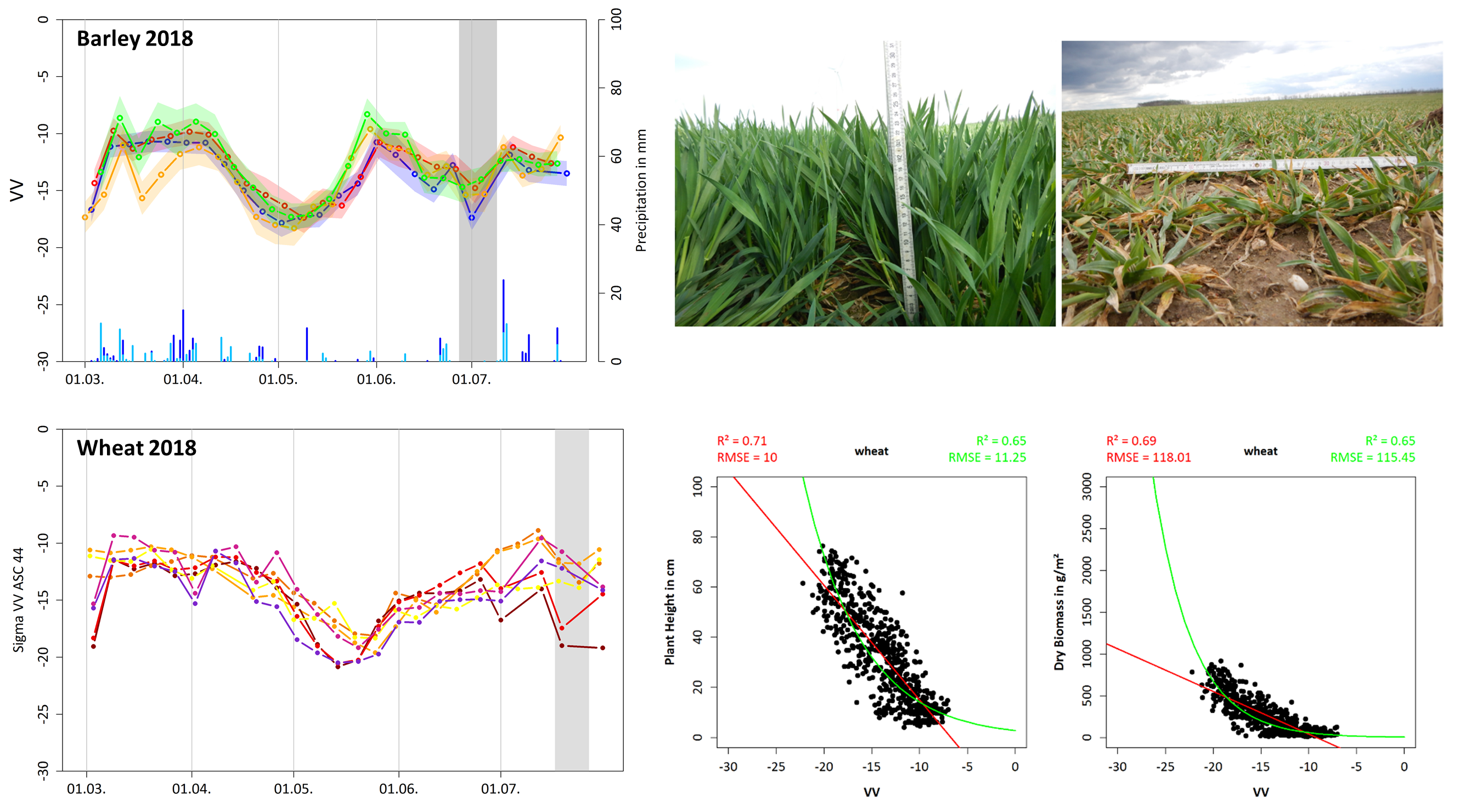
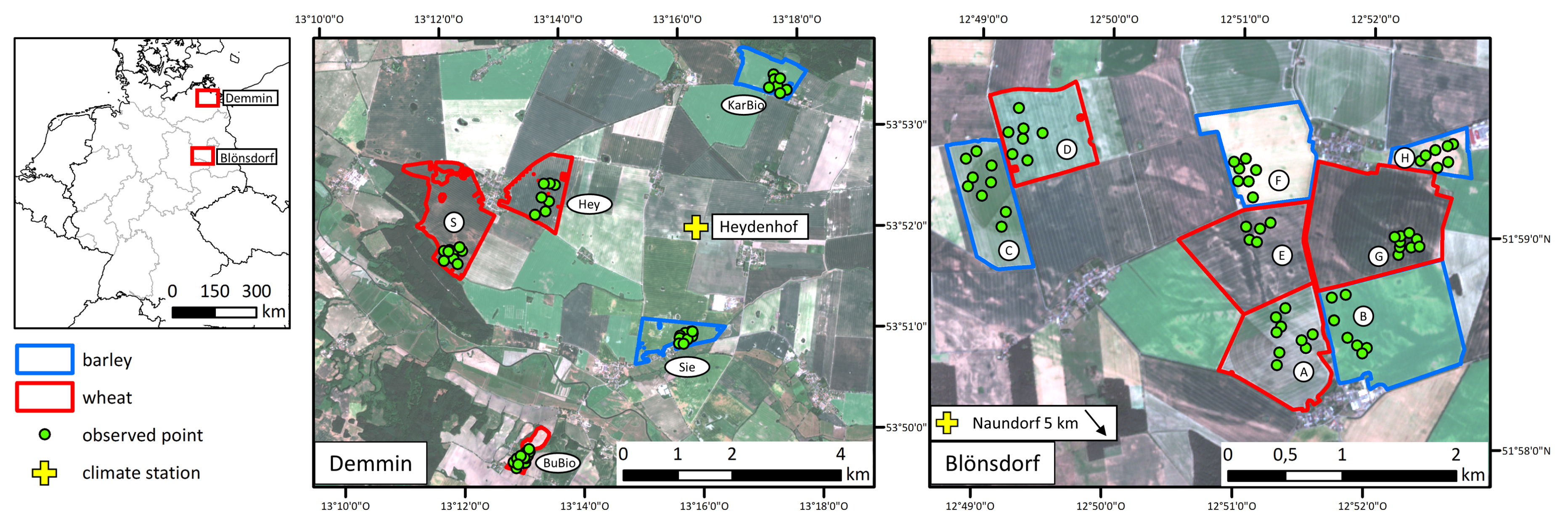
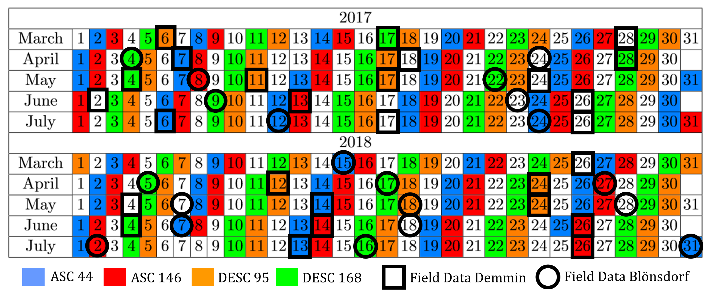
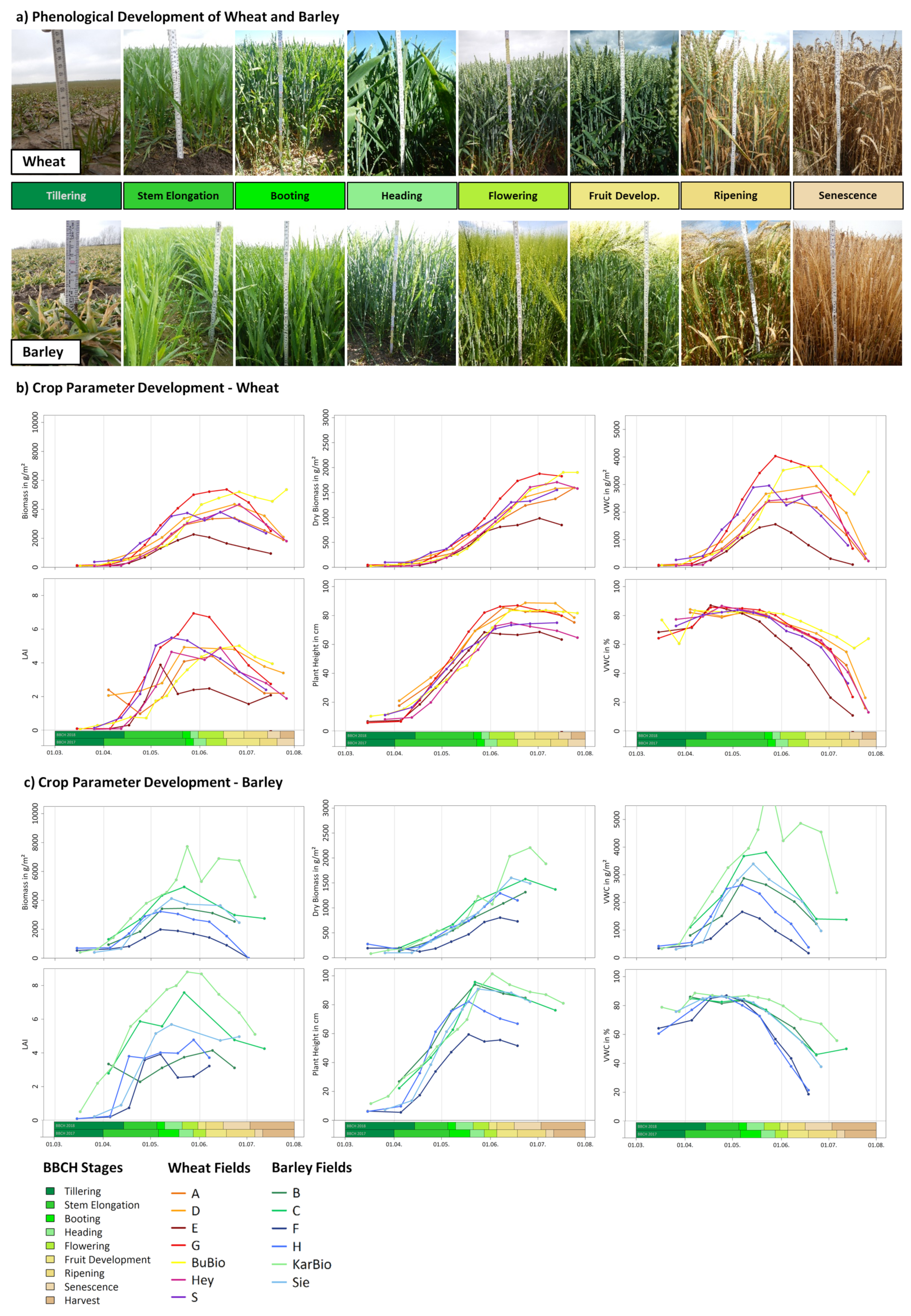
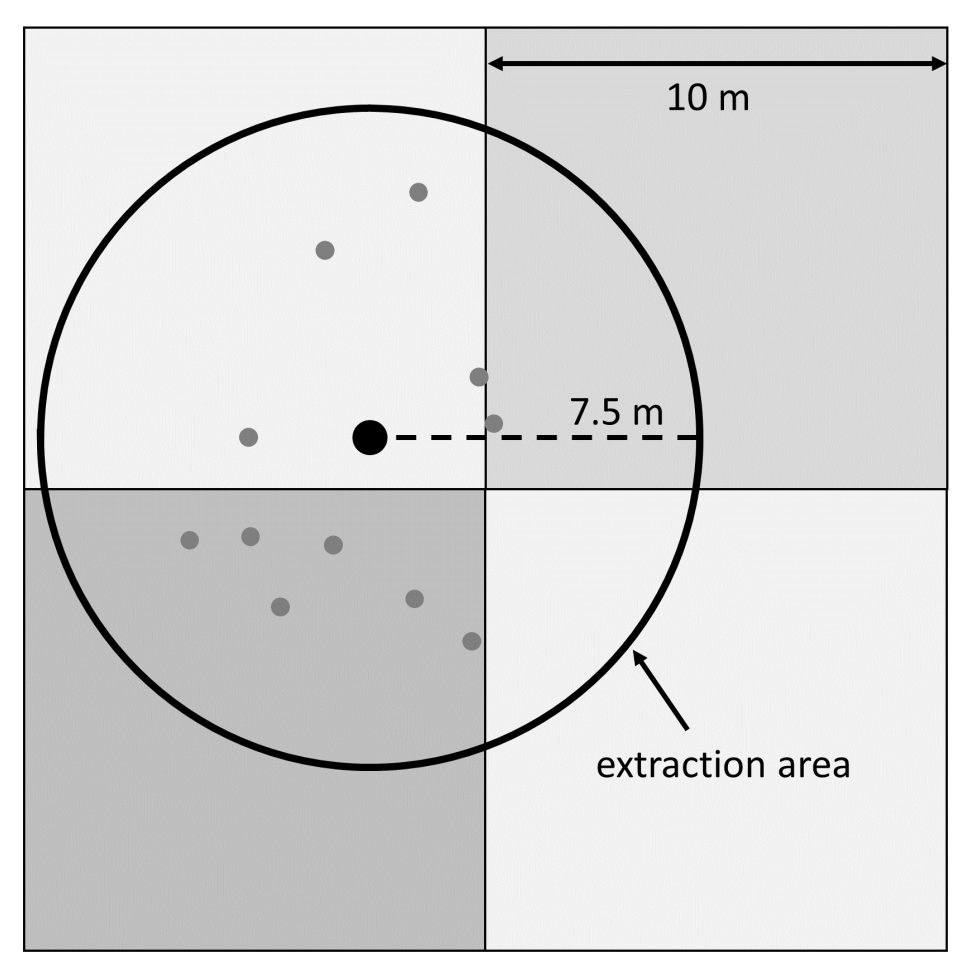
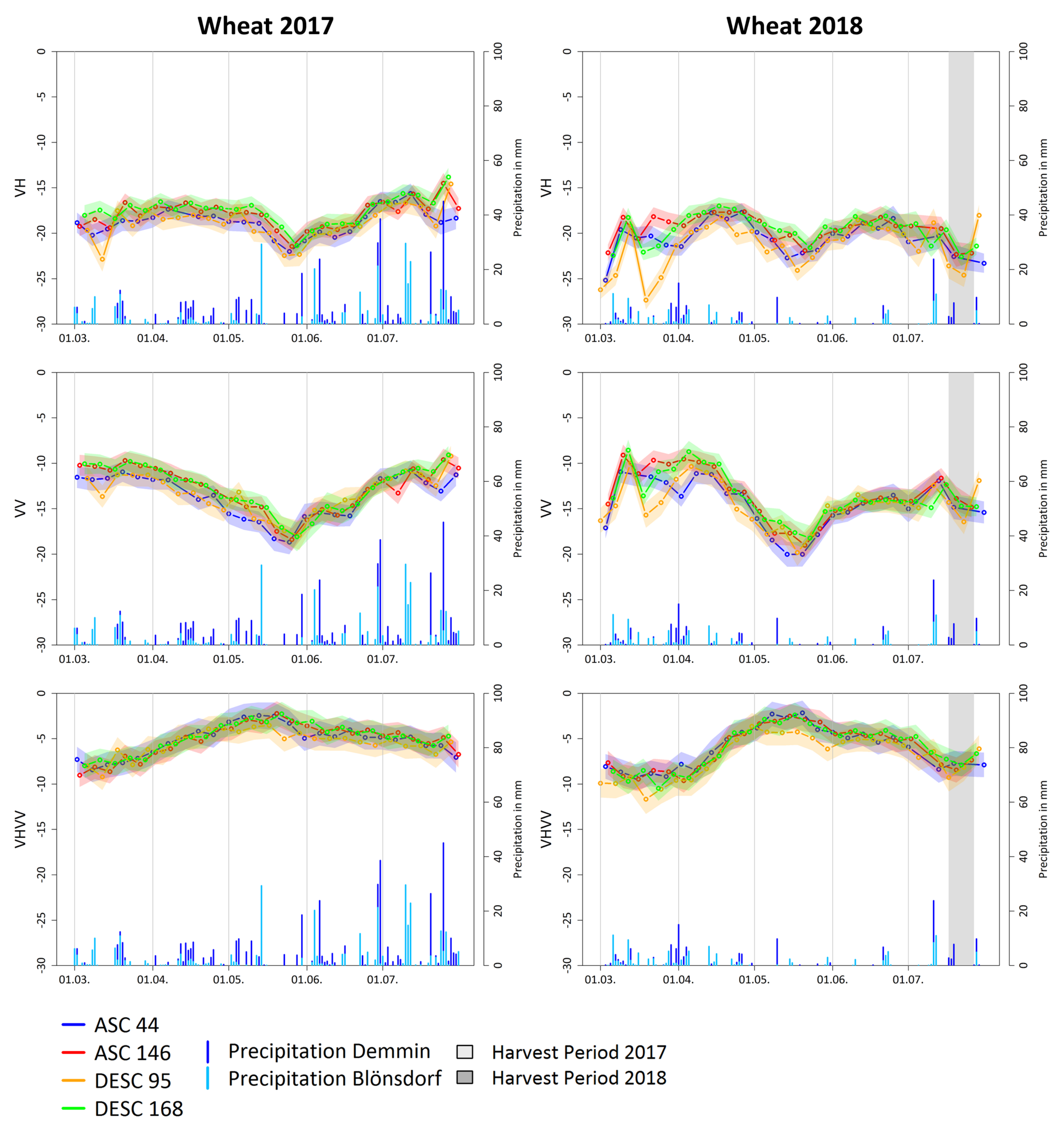
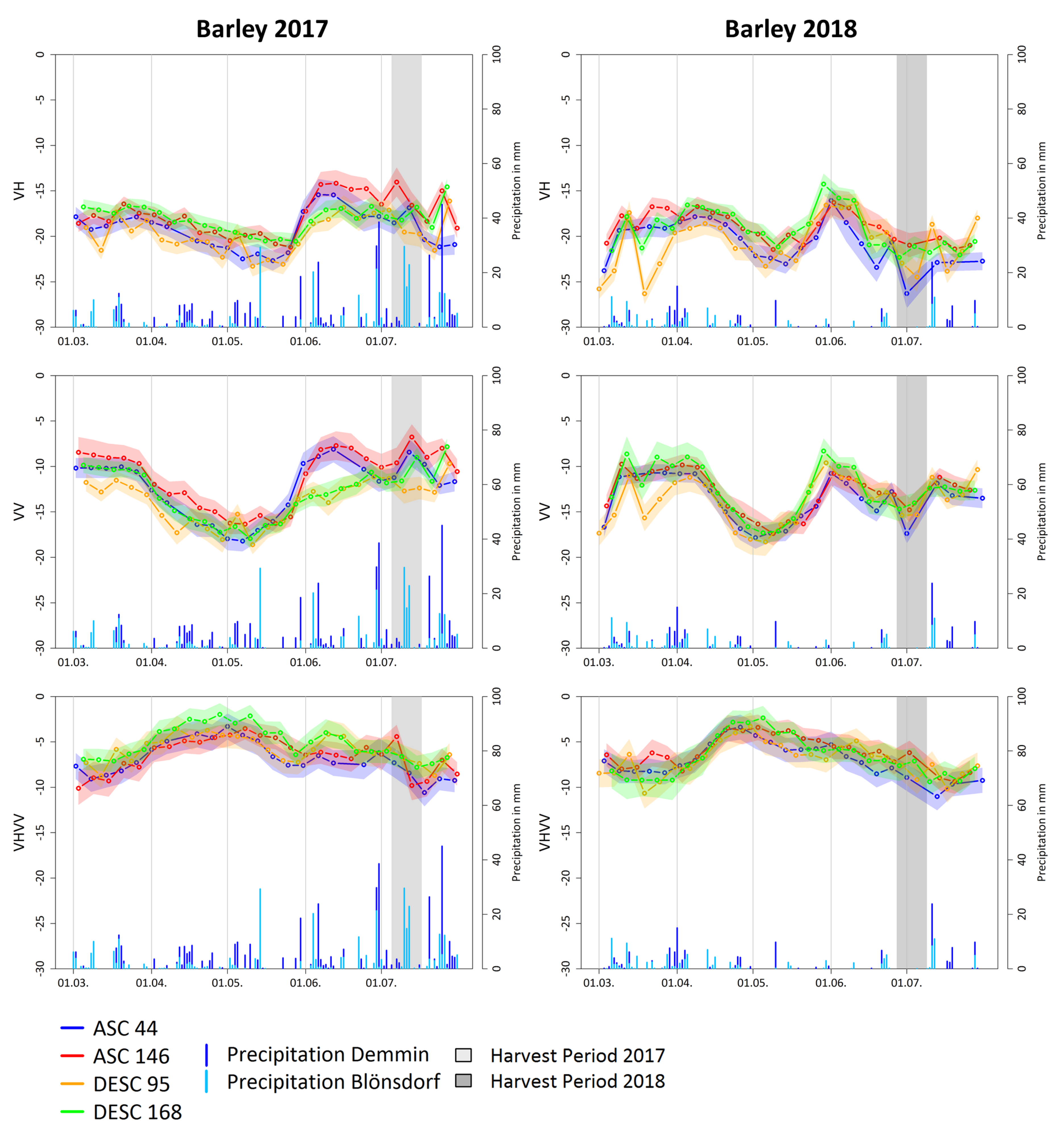
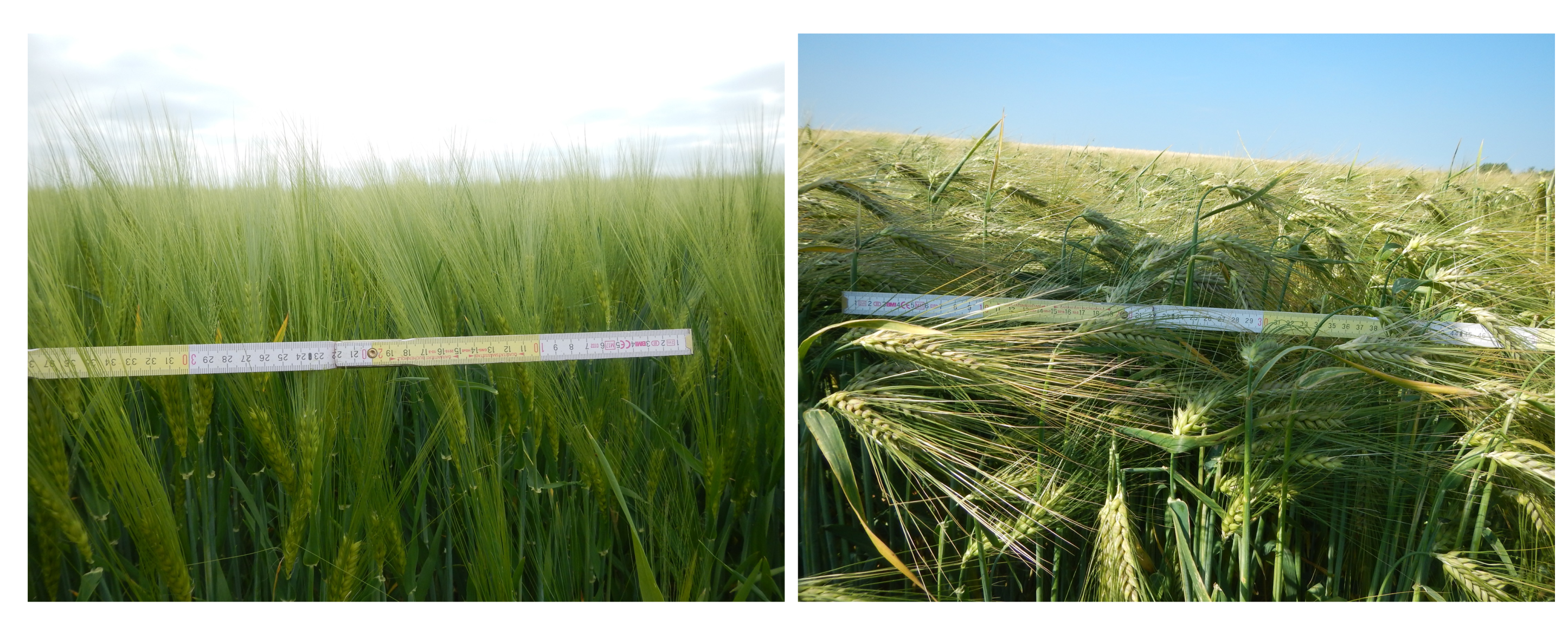
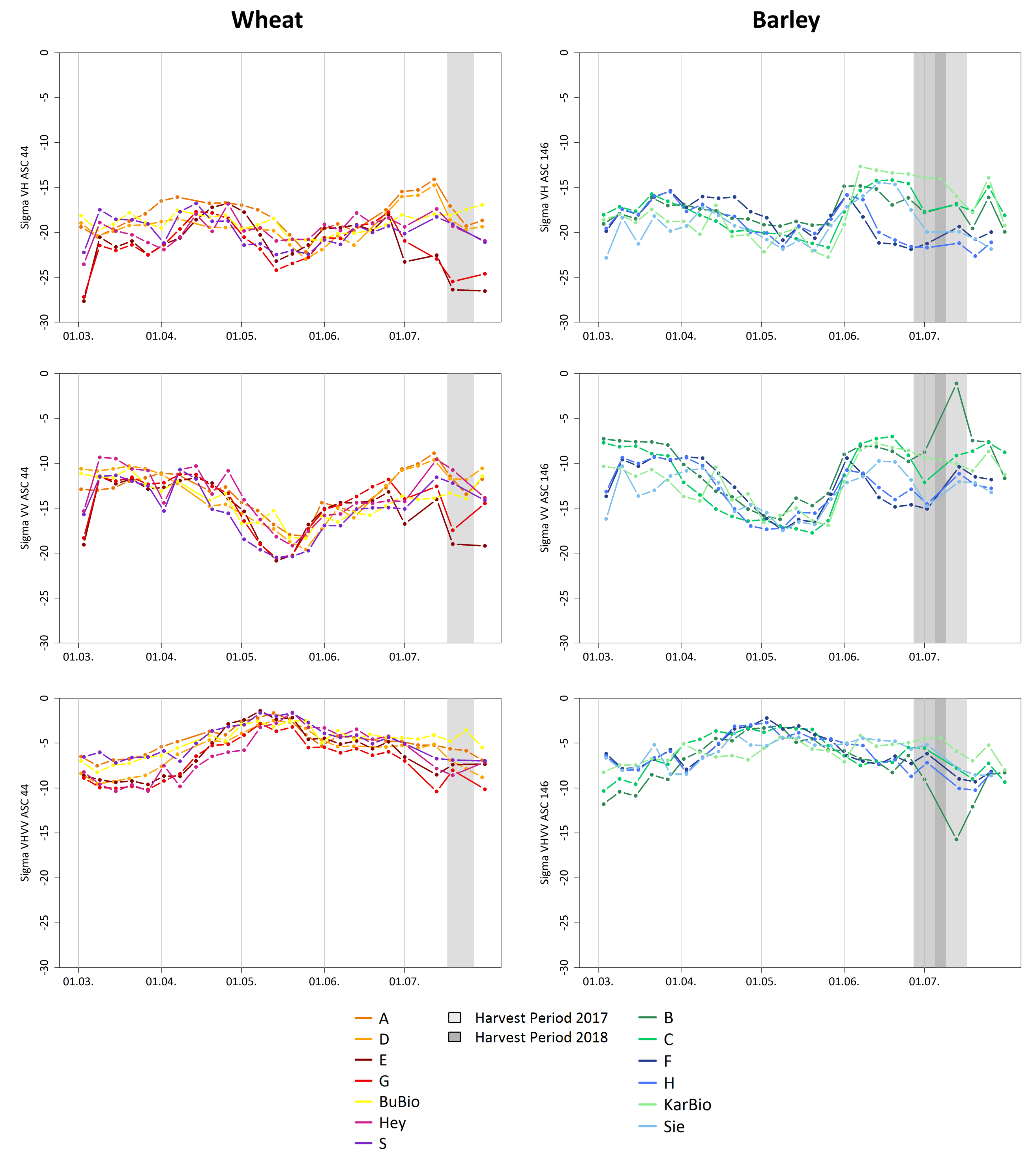
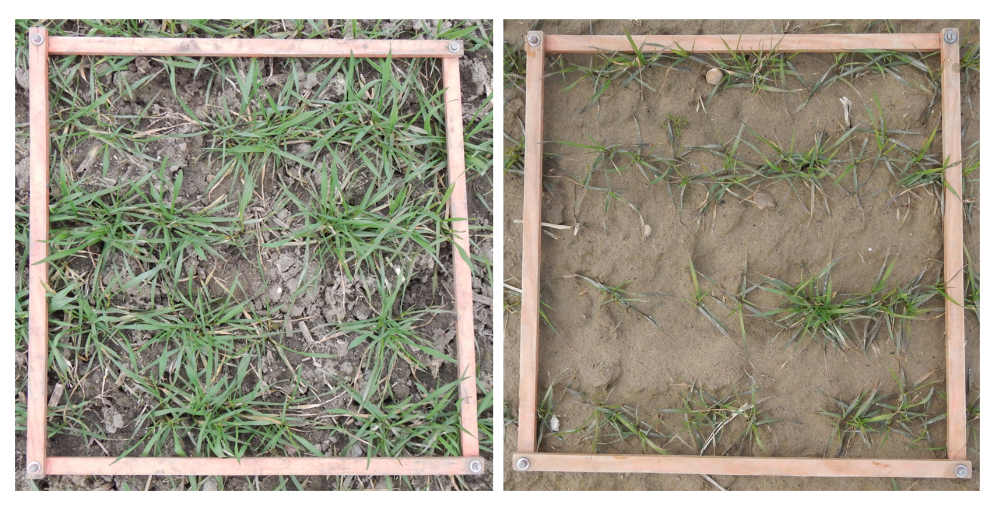
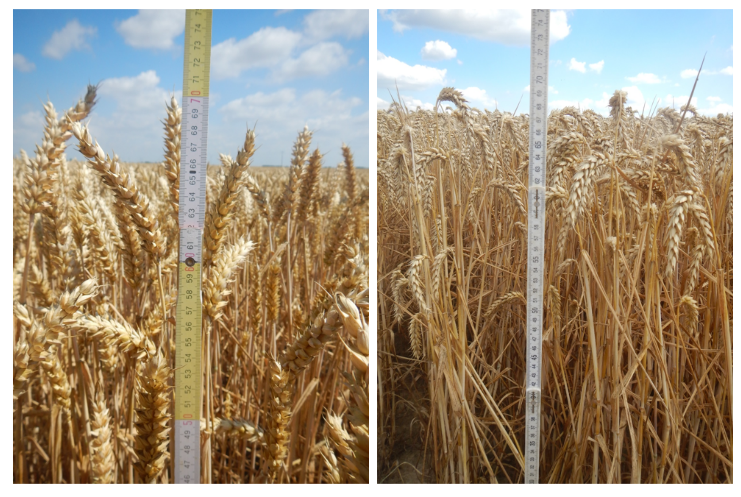
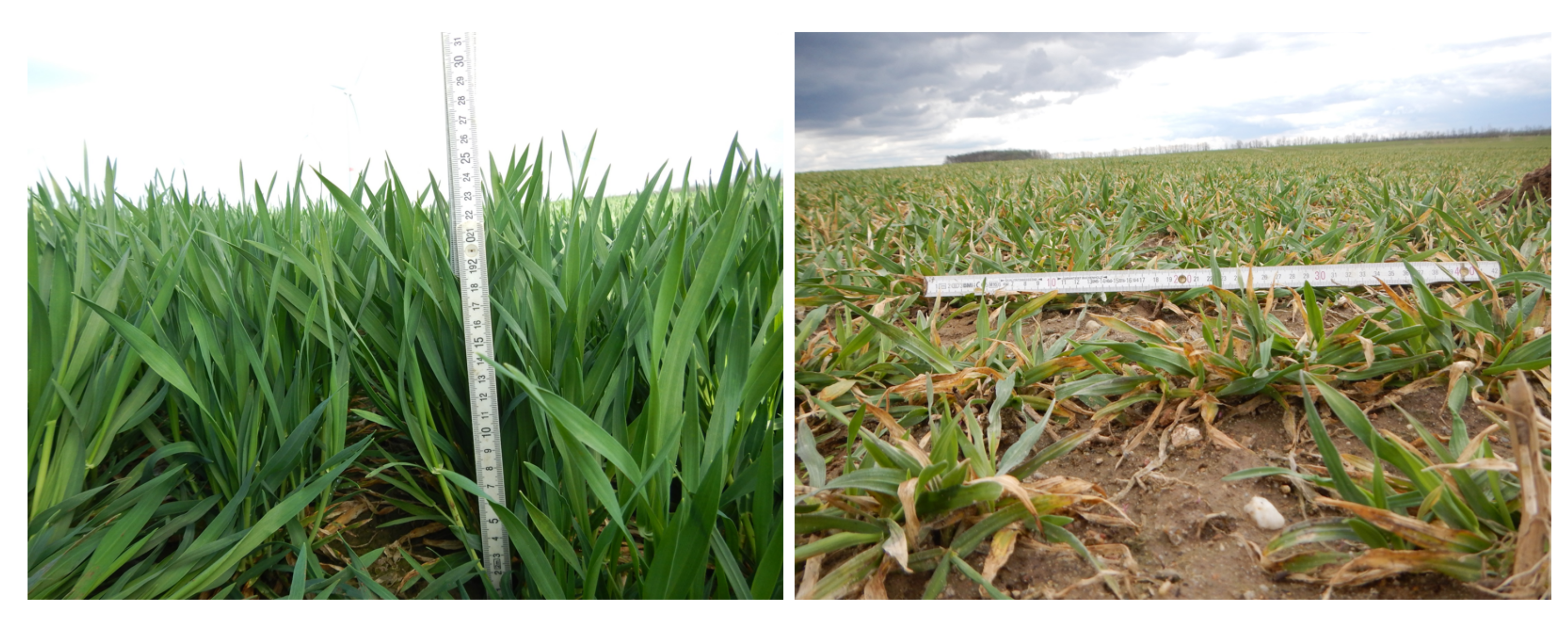
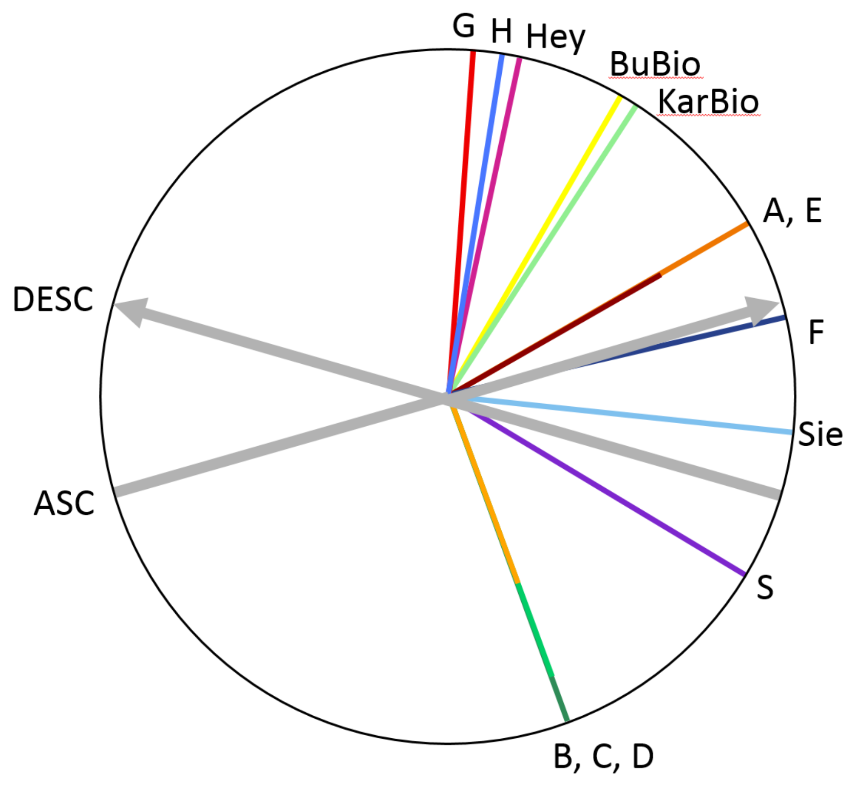
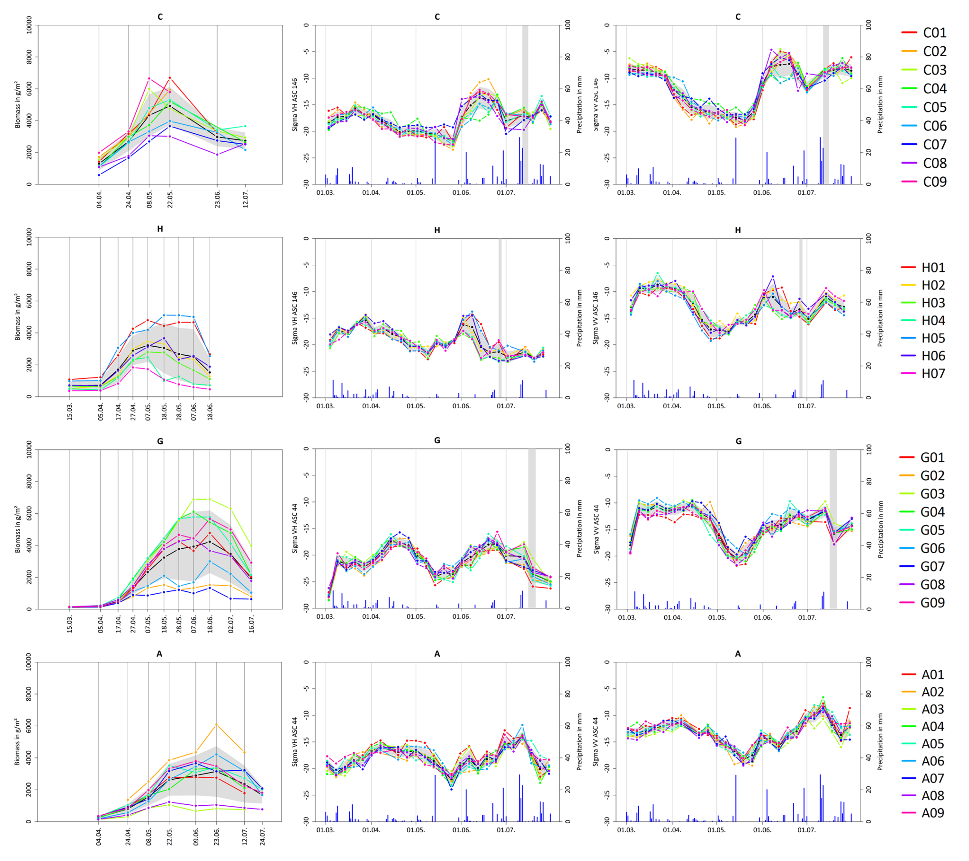
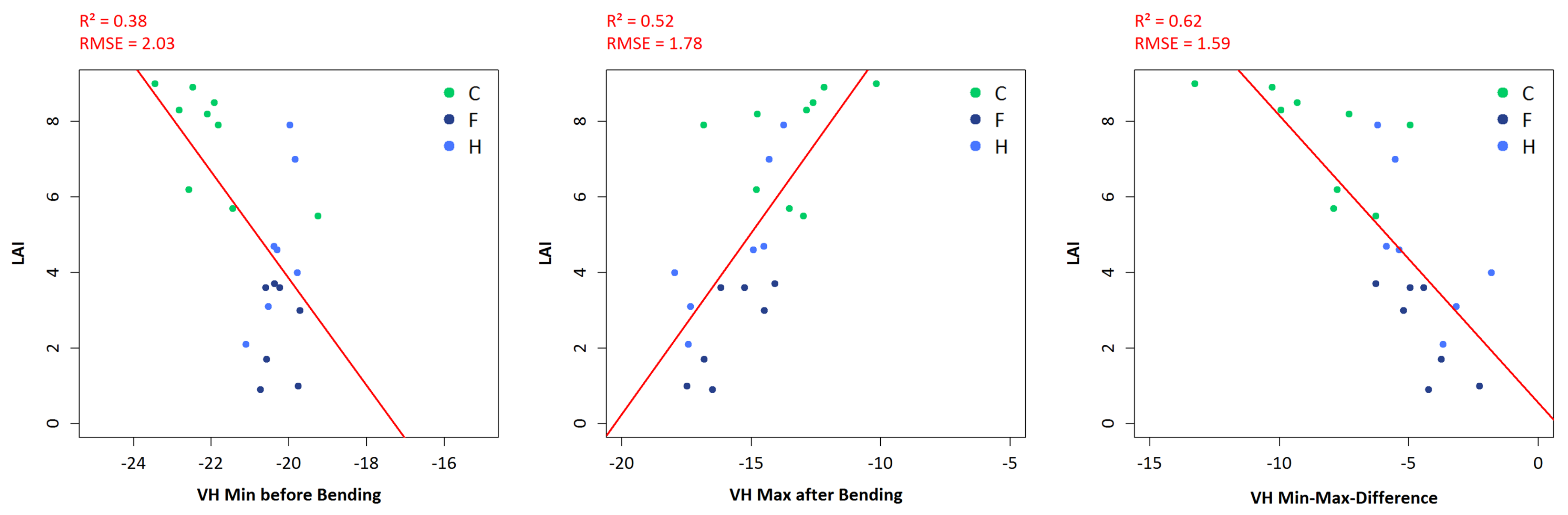
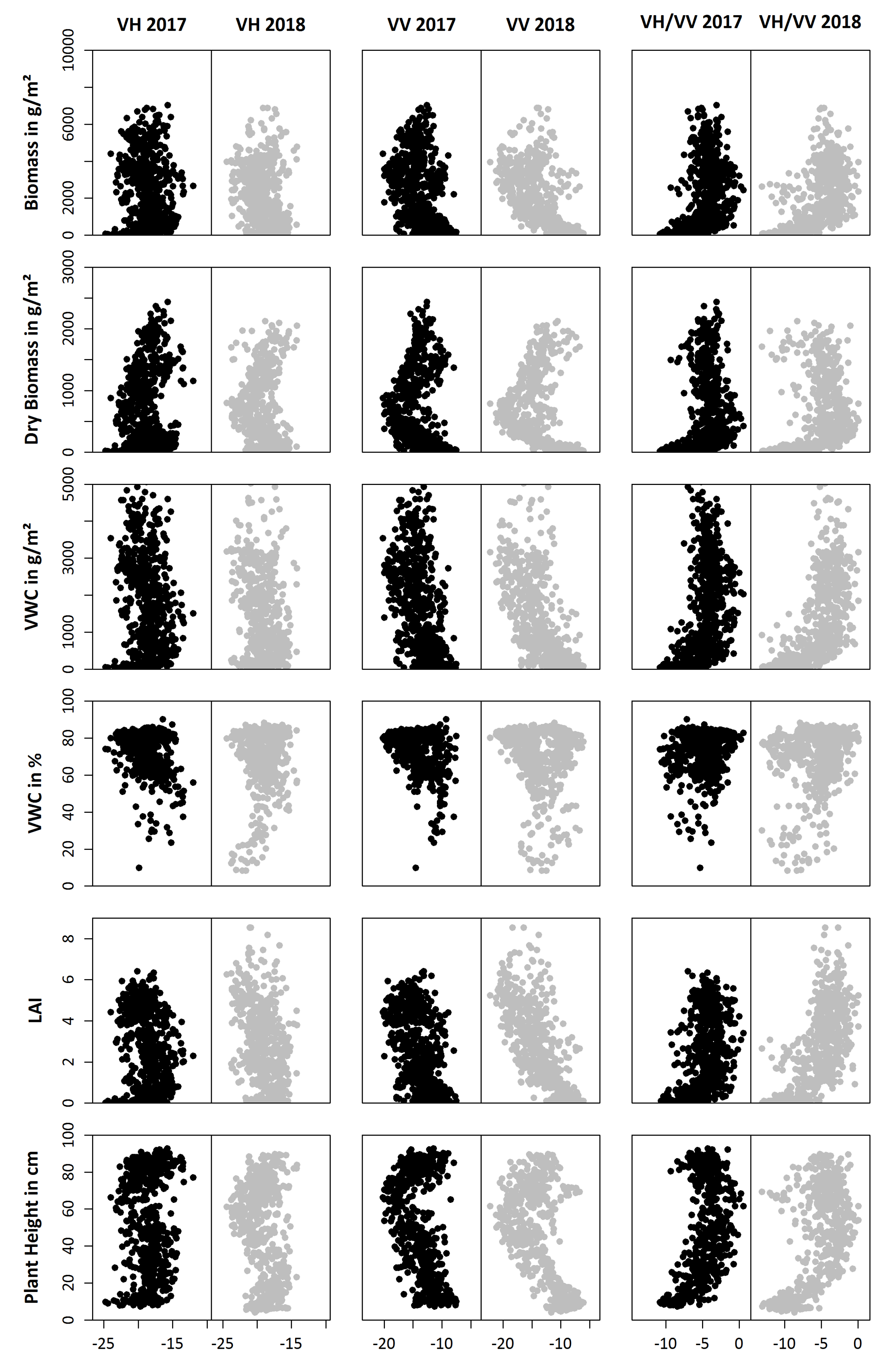
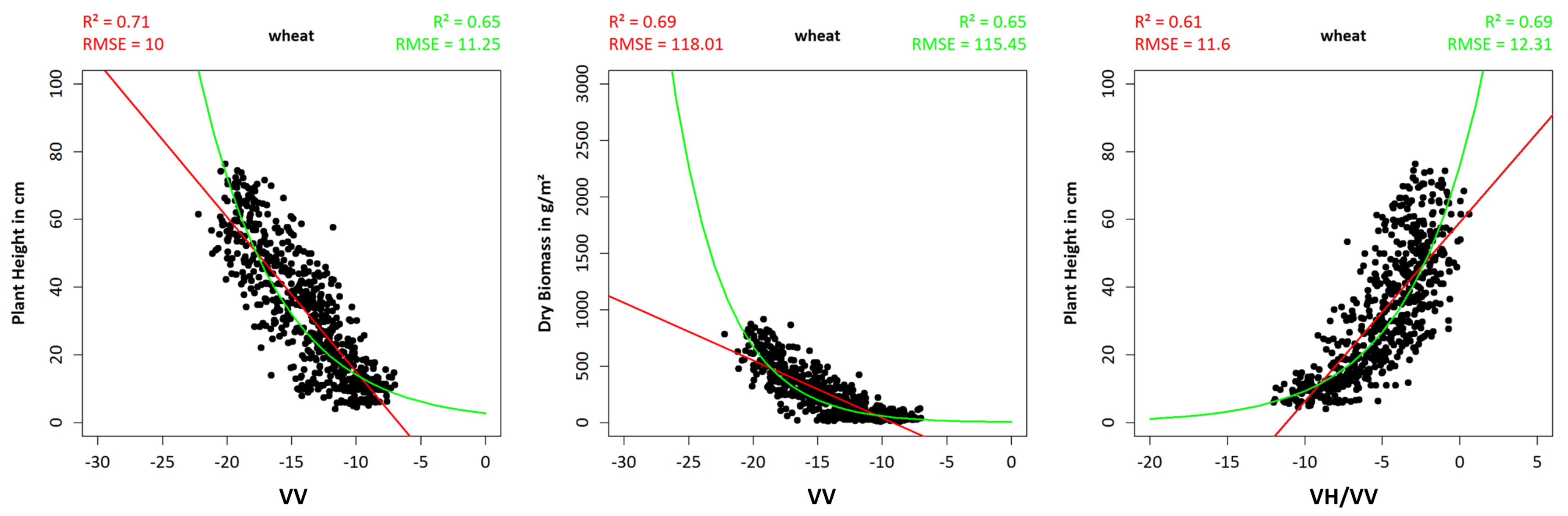
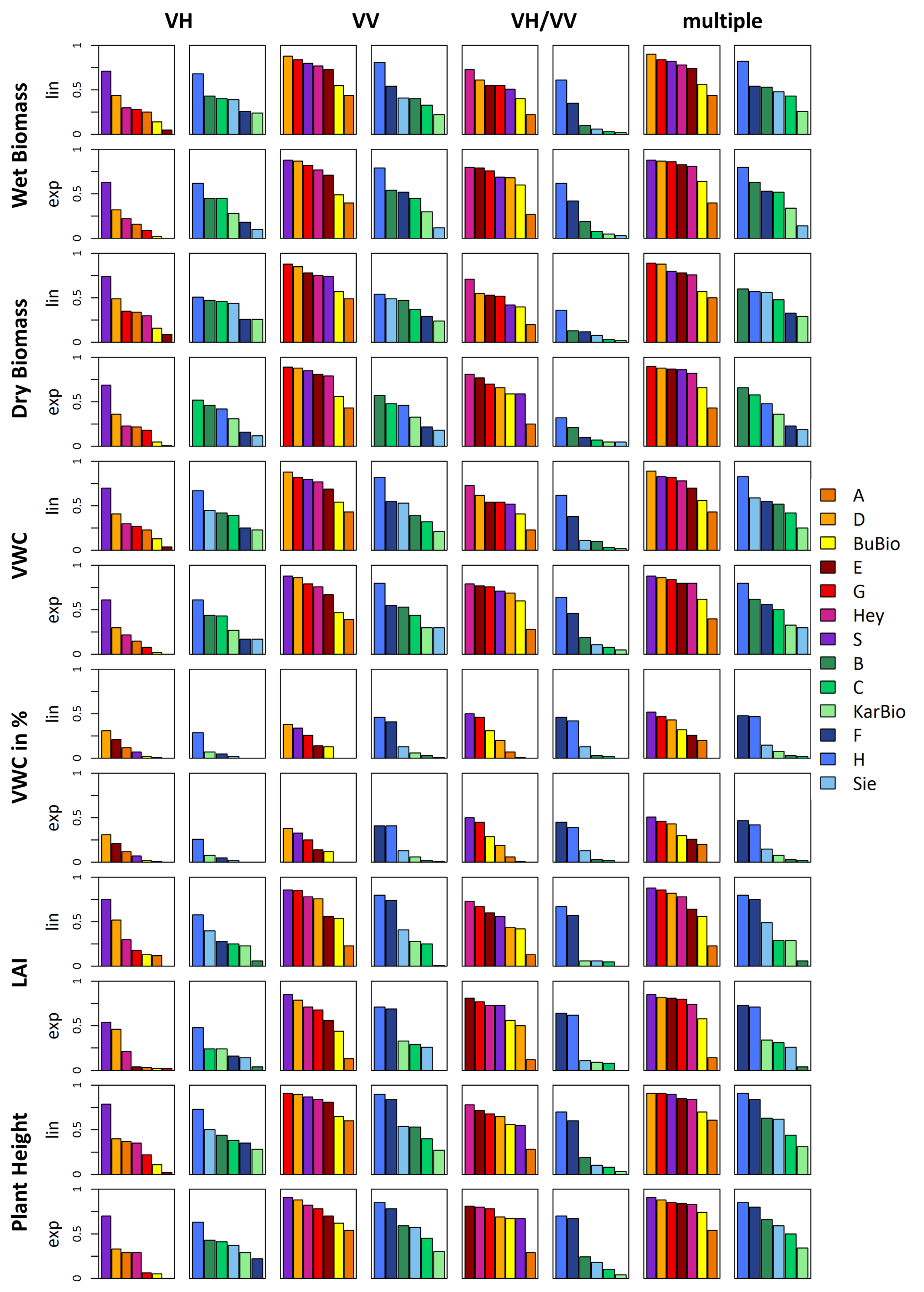
Table 1.
Observed fields in Demmin and Blönsdorf 2017 and 2018.
| Test Site | Year | Field Name | Crop Type | Field Size [ha] | Number of Points | Visits until Harvest | Harvest Period |
|---|---|---|---|---|---|---|---|
| Demmin | 2017 | BuBio | wheat | 23 | 15 | 16 | August |
| KarBio | barley | 71 | 7 | 12 | 17.07–26.07. | ||
| 2018 | S | wheat | 180 | 9 | 10 | 17.07.–25.07. | |
| Hey | wheat | 107 | 7 | 11 | 27.07. | ||
| Sie | barley | 69 | 10 | 8 | 02.07.–05.07. | ||
| Blönsdorf | 2017 | A | wheat | 69 | 9 | 7 | 20.07.– 02.08. |
| B | barley | 103 | 7 | 6 | 05.07.–06.07. | ||
| C | barley | 52 | 9 | 6 | 13.07.–15.07. | ||
| D | wheat | 58 | 7 | 7 | 03.08.–17.08. | ||
| 2018 | E | wheat | 72 | 5 | 11 | 17.07. | |
| F | barley | 66 | 7 | 9 | 29.06. | ||
| G | wheat | 108 | 9 | 11 | 17.07.–26.07. | ||
| H | barley | 20 | 7 | 9 | 27.06. |
Table 2.
Crop Parameters measured during field campaigns 2017 and 2018.
| Crop Parameter (Field) | Unit | Method |
|---|---|---|
| Phenology | Phenological growth stage in BBCH scale [38] | |
| Plant Height | cm | Average height of ca. 10 plants, measured by folding rule |
| Leaf Area Index (LAI) | m/m | Green leaf area per unit ground surface area, average of ca. 10 measurements with SunScan LAImeter |
| Wet Biomass | g/m | Weight of fresh plants, destructive sampling of plants in five 1 m rows |
| Crop Parameter (Lab) | ||
| Dry Biomass | g/m | Weight of oven-dried plants (at 105 C until constant weight) |
| Vegetation Water Content (VWC) | g/m | Weight difference between wet and dry biomass |
| Relative Vegetation Water Content | % | Weight difference between wet and dry biomass divided by wet biomass |
Table 3.
R values of the regression between crop and backscatter parameters per crop type for all fields. Values in parentheses are not significant (p > 0.01).
Table 3.
R values of the regression between crop and backscatter parameters per crop type for all fields. Values in parentheses are not significant (p > 0.01).
| ASC146 all | VH | VV | VH/VV | Multiple | |||||
|---|---|---|---|---|---|---|---|---|---|
| Wheat | Barley | Wheat | Barley | Wheat | Barley | Wheat | Barley | ||
| Wet Biomass | lin | 0.02 | (0) | 0.21 | 0.02 | 0.2 | 0.08 | 0.24 | 0.08 |
| exp | (0) | (0) | 0.33 | 0.02 | 0.41 | 0.11 | 0.42 | 0.11 | |
| Dry Biomass | lin | (0) | 0.16 | 0.03 | 0.07 | 0.06 | 0.01 | 0.06 | 0.17 |
| exp | (0) | 0.04 | 0.22 | (0) | 0.28 | 0.04 | 0.29 | 0.07 | |
| VWC | lin | 0.04 | 0.02 | 0.3 | 0.08 | 0.26 | 0.08 | 0.32 | 0.1 |
| exp | (0) | 0.01 | 0.36 | 0.09 | 0.46 | 0.15 | 0.48 | 0.16 | |
| VWC in % | lin | (0) | 0.14 | 0.05 | 0.2 | 0.06 | 0.06 | 0.06 | (0.2) |
| exp | (0) | 0.07 | 0.03 | 0.12 | 0.06 | 0.06 | 0.06 | 0.12 | |
| LAI | lin | 0.07 | 0.02 | 0.39 | 0.06 | 0.3 | 0.07 | 0.4 | 0.08 |
| exp | 0.01 | 0.02 | 0.38 | 0.1 | 0.46 | 0.15 | 0.48 | 0.16 | |
| Plant Height | lin | (0) | (0.01) | 0.2 | (0.01) | 0.25 | 0.07 | 0.26 | 0.08 |
| exp | (0) | (0) | 0.3 | 0.06 | 0.39 | 0.14 | 0.41 | 0.14 | |
Table 4.
R values of the regression between crop and backscatter parameters per crop type for all fields in BBCH stages 21–49. Values in parentheses are not significant (p > 0.01).
Table 4.
R values of the regression between crop and backscatter parameters per crop type for all fields in BBCH stages 21–49. Values in parentheses are not significant (p > 0.01).
| BBCH 21–49 | VH | VV | VH/VV | Multiple | |||||
|---|---|---|---|---|---|---|---|---|---|
| Wheat | Barley | Wheat | Barley | Wheat | Barley | Wheat | Barley | ||
| Wet Biomass | lin | 0.22 | 0.36 | 0.69 | 0.38 | 0.46 | 0.11 | 0.69 | 0.43 |
| exp | 0.06 | 0.2 | 0.6 | 0.3 | 0.61 | 0.14 | 0.67 | 0.3 | |
| Dry Biomass | lin | 0.23 | 0.32 | 0.69 | 0.35 | 0.44 | 0.11 | 0.68 | 0.39 |
| exp | 0.09 | 0.14 | 0.65 | 0.22 | 0.6 | 0.11 | 0.7 | 0.22 | |
| VWC | lin | 0.22 | 0.38 | 0.68 | 0.41 | 0.45 | 0.12 | 0.68 | 0.46 |
| exp | 0.05 | 0.28 | 0.57 | 0.42 | 0.6 | 0.2 | 0.65 | 0.42 | |
| VWC in % | lin | (0.01) | 0.2 | 0.09 | 0.33 | 0.21 | 0.17 | 0.22 | 0.33 |
| exp | (0.01) | 0.19 | 0.09 | 0.32 | 0.2 | 0.17 | 0.21 | 0.32 | |
| LAI | lin | 0.19 | 0.34 | 0.65 | 0.4 | 0.46 | 0.13 | 0.66 | 0.43 |
| exp | 0.03 | 0.27 | 0.52 | 0.46 | 0.58 | 0.24 | 0.62 | 0.46 | |
| Plant Height | lin | 0.12 | 0.43 | 0.71 | 0.62 | 0.61 | 0.28 | 0.74 | 0.63 |
| exp | 0.05 | 0.39 | 0.65 | 0.64 | 0.69 | 0.33 | 0.75 | 0.65 | |
Table 5.
R values of the regression between crop and backscatter parameters per crop type for all fields in BBCH stages 51–77. Values in parentheses are not significant (p > 0.01).
Table 5.
R values of the regression between crop and backscatter parameters per crop type for all fields in BBCH stages 51–77. Values in parentheses are not significant (p > 0.01).
| BBCH 51–77 | VH | VV | VH/VV | Multiple | |||||
|---|---|---|---|---|---|---|---|---|---|
| Wheat | Barley | Wheat | Barley | Wheat | Barley | Wheat | Barley | ||
| Wet Biomass | lin | (0.02) | (0) | (0.01) | (0) | (0) | (0) | (0.02) | (0) |
| exp | 0.02 | (0) | (0.01) | (0) | (0) | (0) | (0.02) | (0) | |
| Dry Biomass | lin | 0.05 | 0.24 | 0.07 | 0.22 | (0.01) | (0.01) | 0.07 | 0.25 |
| exp | (0.02) | 0.17 | 0.03 | 0.16 | (0.01) | (0.01) | (0.03) | (0.17) | |
| VWC | lin | 0.06 | (0.02) | 0.04 | (0.02) | (0) | (0) | 0.06 | (0.02) |
| exp | 0.05 | (0.01) | 0.04 | (0.02) | (0) | (0.01) | (0.05) | (0.02) | |
| VWC in % | lin | 0.25 | 0.26 | 0.28 | 0.31 | (0.01) | 0.06 | 0.3 | 0.31 |
| exp | 0.23 | 0.19 | 0.27 | 0.25 | (0.02) | 0.06 | 0.28 | 0.25 | |
| LAI | lin | 0.08 | (0) | 0.08 | (0) | (0) | (0) | (0.09) | (0) |
| exp | 0.08 | (0.01) | 0.07 | (0.01) | (0) | (0) | (0.08) | (0.01) | |
| Plant Height | lin | (0) | (0.01) | (0.01) | (0.02) | (0) | (0.01) | (0.01) | (0.02) |
| exp | (0) | (0.01) | (0) | (0.01) | (0) | (0.01) | (0) | (0.01) | |
Table 6.
R values of the regression between crop and backscatter parameters per crop type for all fields in BBCH stages 83–99. Values in parentheses are not significant (p > 0.01).
Table 6.
R values of the regression between crop and backscatter parameters per crop type for all fields in BBCH stages 83–99. Values in parentheses are not significant (p > 0.01).
| BBCH 83–99 | VH | VV | VH/VV | Multiple | |||||
|---|---|---|---|---|---|---|---|---|---|
| Wheat | Barley | Wheat | Barley | Wheat | Barley | Wheat | Barley | ||
| Wet Biomass | lin | 0.23 | 0.47 | (0.01) | 0.27 | 0.13 | 0.2 | 0.24 | 0.47 |
| exp | 0.26 | 0.56 | (0.06) | 0.34 | (0.06) | 0.23 | 0.26 | 0.56 | |
| Dry Biomass | lin | 0.1 | 0.44 | 0.1 | 0.23 | (0) | 0.21 | (0.14) | 0.44 |
| exp | 0.09 | 0.45 | 0.11 | 0.24 | (0) | 0.22 | (0.14) | 0.45 | |
| VWC | lin | 0.25 | 0.43 | (0) | 0.27 | 0.23 | 0.17 | 0.3 | 0.43 |
| exp | 0.44 | 0.57 | (0.07) | 0.39 | 0.16 | 0.2 | 0.44 | 0.58 | |
| VWC in % | lin | 0.43 | 0.51 | (0) | 0.38 | 0.35 | 0.14 | 0.51 | 0.52 |
| exp | 0.5 | 0.46 | (0.02) | 0.36 | 0.29 | 0.12 | 0.53 | 0.48 | |
| LAI | lin | 0.13 | (0.1) | 0.23 | (0.01) | (0.01) | 0.17 | 0.24 | 0.19 |
| exp | (0.09) | (0.09) | 0.22 | (0.01) | (0.03) | 0.2 | 0.22 | 0.21 | |
| Plant Height | lin | 0.1 | 0.4 | (0) | 0.23 | (0.07) | 0.18 | 0.11 | 0.4 |
| exp | (0.06) | 0.35 | (0) | 0.2 | (0.04) | 0.16 | 0.07 | 0.35 | |
© 2019 by the authors. Licensee MDPI, Basel, Switzerland. This article is an open access article distributed under the terms and conditions of the Creative Commons Attribution (CC BY) license (http://creativecommons.org/licenses/by/4.0/).
Share and Cite
MDPI and ACS Style
Harfenmeister, K.; Spengler, D.; Weltzien, C. Analyzing Temporal and Spatial Characteristics of Crop Parameters Using Sentinel-1 Backscatter Data. Remote Sens. 2019, 11, 1569. https://0-doi-org.brum.beds.ac.uk/10.3390/rs11131569
AMA Style
Harfenmeister K, Spengler D, Weltzien C. Analyzing Temporal and Spatial Characteristics of Crop Parameters Using Sentinel-1 Backscatter Data. Remote Sensing. 2019; 11(13):1569. https://0-doi-org.brum.beds.ac.uk/10.3390/rs11131569
Chicago/Turabian StyleHarfenmeister, Katharina, Daniel Spengler, and Cornelia Weltzien. 2019. "Analyzing Temporal and Spatial Characteristics of Crop Parameters Using Sentinel-1 Backscatter Data" Remote Sensing 11, no. 13: 1569. https://0-doi-org.brum.beds.ac.uk/10.3390/rs11131569
Note that from the first issue of 2016, this journal uses article numbers instead of page numbers. See further details here.