Influence of Scanner Position and Plot Size on the Accuracy of Tree Detection and Diameter Estimation Using Terrestrial Laser Scanning on Forest Inventory Plots

Abstract

This research tested how different scanner positions and sample plot sizes affect the tree detection and diameter measurement in forest inventories. For this, a multistage density-based clustering approach was further developed for the automatic mapping of tree positions and simultaneously applied with automatic measurements of tree diameters. This further development of the algorithm reduced the proportion of falsely detected tree locations by about 64%. The algorithms were tested in different settings with respect to the number and spatial alignment of scanner positions and under manifold forest conditions, covering different age classes and a mixture of scenarios, and representing a broad gradient of structural complexity. For circular sample plots with a maximum radius of 20 m, the tree mapping algorithm showed a detection rate of 82.4% with seven scanner positions at the vertices of a hexagon plus the center coordinates, and 68.3% with four scanner positions aligned in a triangle plus the center. Detection rates were significantly increased with smaller maximum radii. Thus, with a maximum radius of 10 m, the hexagon setting yielded a detection rate of 90.5% and the triangle 92%. Other alignments of scanner positions were also tested, but proved to be either unfavorable or too labor-intensive. The commission rates were on average less than 3%. The root mean square error (RMSE) of the dbh (diameter at breast height) measurement was between 2.66 cm and 4.18 cm for the hexagon and between 3.0 cm and 4.7 cm for the triangle design. The robustness of the algorithm was also demonstrated via tests by means of an international benchmark dataset. It has been shown that the number of stems per hectare had a significant impact on the detection rate.

1. Introduction

The major purpose of forest inventories is to provide relevant information on the status and changes of forest landscapes. Forest inventory data not only are required for decision making in forest management, but also are used as an empirical platform for manifold research activities. In order to provide reliable and precise information on traditional attributes, such as average growing stock timber volume or tree count, measurement errors besides the design-based sampling variance should be kept as small as possible.

In traditional forest inventories with multiple sample plots, tree attributes and positions are manually measured using mechanical or optical instruments such as calipers, hypsometers, compasses, and measuring tapes [1,2,3,4]. The application of these traditional measurement techniques is time-consuming, cost-intensive, and prone to manifold measurement errors [5,6,7]. Recorded tree positions are often imprecise, as position, distance, and angle errors propagate, especially on rough terrain [8,9]. Trials to improve efficiency since the beginning of forest inventory have permanently enhanced techniques, instruments, and protocols [6].

In recent years, terrestrial laser scanner (TLS) systems have been successfully applied in the context of forestry applications (e.g., [5,7,10,11,12,13,14,15,16,17,18,19]). Using TLS, the structure of both vegetation and terrain can be automatically measured by means of massive clouds of XYZ points in 3D space [5]. A major benefit of TLS is the fast, automatic, and detailed registration of the forest structure [20]. Because TLS technology is associated with novel standards and protocols, it is gradually influencing traditional methodology in the evaluation of forest structure attributes [10,21,22]. The main purpose of TLS-based research activities in the context of forest inventories is to enhance labor efficiency and replace manual measurements by automatic methods [5,7,16]. Early studies on the application of TLS in forest inventories revealed its high potential to derive precise measurements of single tree attributes (e.g., [5,23,24,25,26]), but much effort is still required to analyze the TLS data. If the aim is to extract single tree attributes, for example, diameter or height, by fully automatic routines from 3D point clouds, it is mandatory to detect the true tree locations in an initial step prior to further data processing. Nowadays, several approaches have been proposed for the automatic detection of tree positions. The most relevant approaches can be classified into cluster algorithms and circle- or cylinder-fitting algorithms (e.g., [27,28,29,30]). Because 3D point cloud data from TLS are often too large for efficient computation, either the point cloud is discretized into voxels (e.g., [31,32]) or clustering is subsequently applied to subsamples from multiple vertical layers (e.g., [7,33,34]).

Several studies have focused on the automatic detection of trees in a forest inventory context. In single scan mode, where only one scan is carried out in the plot center, up to 40% of trees cannot be detected [5,6,34,35,36,37,38,39,40,41]. For multiple scan mode, the literature describes various scanner location patterns. In principle, the following setup patterns are distinguished: (i) the scanner positions are located at the edges of the sample plot [12,42,43,44,45,46], (ii) the scanner positions are outside the sample plot [13,26,46,47], or (iii) one scanner position is in the center and the rest are more or less evenly distributed around it [6,39,46,48,49,50,51,52,53,54]. Abegg et al. [46] showed, in a comprehensive simulation study on the impact of scanner location on occlusion, that an intuitive distribution of scanner positions within the sample point with similar distances between the positions and edges of the sample plot ensures the best overall visibility of the stand.

Major findings of selected recent studies are described as follows. Heinzel and Huber [53] were able to detect 97.4% of tree positions with a diameter at breast height (dbh) greater or equal to 12 cm with five scanner positions on plots with 7.98 m radius. Further, 97.3% of tree positions were detected for dbhs greater or equal to 36 cm on plots with a 12.62 m radius. For a random selection and arbitrary number of regeneration trees with a dbh lower than 12 cm, a detection rate of 84.6% was achieved. Using single scan mode, Reddy et al. [39] detected 77.8% and 91% of the trees (dbh > 9.5 cm with 400–500 stems per hectare) on circular plots with a radius of 20 m and 10 m, respectively. Using multiscan mode with five scanner positions on the same plots, 96.5% and 100% of the trees were consequently detected. Oveland et al. [40] achieved an average detection rate of 61.8% (dbh > 4 cm, 380–1380 stems per hectare) in single scan mode on plots with a 12.62 m radius. With five scanner positions, Liu et al. [54] detected between 72.5% and 100% of the trees given different plot sizes, dbh-limits, and stem numbers. In a review paper, Liang et al. [5] showed that detection rates were between 22% and 100% in single scan mode and between 62.1% and 100% in multiple scan mode. In summary, many studies (e.g., [5,6,13,22]) have shown that detection rates are highly influenced by the forest structure, as well as by the number of scans and the position of the scanner. As a general finding, the proportion of correctly detected trees decreases with increasing stem density and increasing plot size, and increases with increasing mean dbh and an increasing number of scanner positions.

Automatic dbh measurement or, in general, measurement of diameter in arbitrary stem heights is most commonly conducted via circle- or cylinder-fitting algorithms. This step is either carried out simultaneously with the tree detection (e.g., [55]) or subsequently performed based on the detected tree locations (e.g., [7,31]). Recent studies indicate that dbh can be measured with a root mean square error (RMSE) between 0.7 cm and 13.35 cm and a bias between 0.4 cm and 2 cm [39,40,41,56,57,58,59]. The relative RMSE varied between 4.4% and 28.6% and the relative bias between 0.3% and 9.2%. The review paper of Liang et al. [5] reports RMSE ranging from 0.7 cm to 7 cm (relative RMSE from 3.9% to 17.5%) and bias ranging from 0.2 cm to 1.6 cm (relative bias from 0.9% to 4%).

It turns out that, owing to the many possible combinations of parameter settings, such as hardware properties, scanner position variations, underlying forest structure diversity, and nonhomogeneous quality criteria, a comparative assessment of the results from the different TLS studies is difficult [6]. For this reason, an international benchmark project [6] was initiated in order to evaluate the performance of different algorithms under predefined reference conditions. With regard to the forest structure, the benchmark data were divided into “easy”, “medium”, and “difficult” plots. Furthermore, as consistent quality criteria, “completeness” (detection rate) and “correctness”, and “mean accuracy” as a combination of the two, were defined. Within the concerted activities of the benchmark project, the mean accuracy achieved with the different approaches using a multiscan setting ranged between 74% and 53% under medium and difficult conditions, respectively [6].

Despite the promising benefits of TLS, in terms of providing high-resolution 3D information, a gold standard approach for automatic tree detection and stem diameter measurement is still lacking. Consequently, TLS is so far not exclusively used as a standard measurement technique in forest inventory practice. This is especially because even well-performing approaches generally show high variance with respect to the quality criteria and when tested with different scanner settings and under various forest structure scenarios.

The goal of the present study was to investigate the influence of scanner position and plot size on the accuracy of tree detection and diameter estimation in forest inventory. In the course of this, an algorithm for the automatic detection of stems, which has been successfully used for the mapping of complete forest stands in a forest monitoring context [7], was further developed. The aim of this further algorithm development is to reduce the proportion of falsely detected tree locations. The enhanced multistage clustering algorithm was tested on smaller forest inventory sample plots with varying scanner positions and numbers of scans. It was also examined how the accuracy of automatic stem detection was influenced by the structural diversity of the forest. Finally, the algorithm was applied to reference data provided by the international benchmark project in the work of [6].

2. Data and Methods

2.1. Study Area and Sample Plots

The BOKU Institute of Forest Growth maintains a permanently repeated forest inventory in the forest district of Ofenbach located in the federal state of Lower Austria near the village of Forchtenstein. The forest inventory was initiated by Schodterer [60] in 1989 and comprises a total of 554 sample plot locations. Sample plots are systematically aligned in a regular grid with a mesh width of 141.4 m $\times$ 141.4 m. At each sample point, Bitterlich relascope sampling [61,62,63] was conducted using a constant basal area factor of 4 m² per ha. Trees were recorded only if their dbh (measured from one direction with caliper in 1.3 m height) was greater than or equal to a lower threshold of 5 cm. For the present study, a subsample of 23 plots was selected in such a way that possible variations in forest type (broadleaved, coniferous, and mixed), forest structure, and terrain property (flat to steep) were represented. The Bitterlich method produces an incomplete tree pattern that results from a size-related and distance-dependent thinning. In order to obtain reference information on the existing trees that were thinned by the Bitterlich process, their positions and dbh (measured from one direction in 1.3 m height) were manually measured in the 3D point cloud. By doing so, only trees with a dbh of 5 cm or greater and a distance of 20 m or less from the sample plot center were measured. In addition, covariates were derived for each sample plot, among them mixture type, main species, Shannon index [64], existence of regeneration, and terrain slope. Using the sample tree data, further attributes were derived: basal area per hectare ($BA/ha$), quadratic mean diameter ($dm$), stand density index ($SDI$) [65], stem density in terms of number of trees per hectare ($N/ha$), coefficient of variation of diameter at breast height ($CVdbh$), dbh differentiation according to Füldner [66] ($Diff\_Fuel$), Clark and Evans aggregation index [67] ($CE$), and proportion of deciduous trees ($p\_dec)$.

Table 1. Summary statistics of sample plots. $slope$, slope of sample plot; $dm$, diameter of mean basal area tree; $BA/ha$, basal area per hectare; $N/ha$, number of trees per hectare; $SDI$, stand density index; $CVdbh$, coefficient of variation of diameter at breast height; $Diff\_Fuel$, dbh differentiation according to Füldner; $CE$, Clark and Evans aggregation index; $shannon$, Shannon index; $p\_dec$, proportion of deciduous trees.

# Of Sample Plots	23
# Of Trees	3894
# Of Trees/Sample Plot	169.3
dbh Range (cm)	5.0–79.6
	Mean	SD	Min	Max
$slope$ (%)	27.8	10.4	10.5	51.0
$dm$ (cm)	22.4	8.3	9.7	37.6
$BA/ha$ (m2/ha)	46.8	10.2	25.7	64.9
$N/ha$ (trees/ha)	1953	1753	279	5658
$SDI$ (trees/ha)	1045	314	523	1648
$CVdbh$	0.79	0.23	0.44	1.43
$Diff\_Fuel$	0.46	0.06	0.28	0.56
$CE$	0.84	0.12	0.63	1.12
$shannon$	0.52	0.38	0	1.16
$p\_dec$	0.38	0.34	0	1

shows summary statistics (number of trees, mean, standard deviation, min, and max) of the metric sample plot parameters. A complete description of the 23 sample plots can be found in Appendix A,

Table A1. Plot descriptions of the 23 sample plots. Summary statistics of sample plots. $slope$, slope of sample plot; $dm$, diameter of mean basal area tree; $BA/ha$, basal area per hectare; $N/ha$, number of trees per hectare; $SDI$, stand density index; $CVdbh$, coefficient of variation of diameter at breast height; $Diff\_Fuel$, dbh differentiation according to Füldner; $CE$, Clark and Evans aggregation index; $shannon$, Shannon index; $\mathrm{p}\_\mathrm{dec}$, proportion of deciduous trees.

Plot	Forest Type	Main Species	Stand Class	Regen- eration	$\mathit{S}\mathit{l}\mathit{o}\mathit{p}\mathit{e}(\%)$	$\mathit{d}\mathit{m}\left(\mathbf{cm}\right)$	dbh Range (cm)	$\mathit{B}\mathit{A}/\mathit{h}\mathit{a}({\mathbf{m}}^2/\mathbf{ha})$	$\mathit{N}/\mathit{h}\mathit{a}(\mathbf{trees}/\mathbf{ha})$	$\mathit{S}\mathit{D}\mathit{I}(\mathbf{trees}/\mathbf{ha})$	$\mathit{C}\mathit{V}\mathit{d}\mathit{b}\mathit{h}$	$\mathit{D}\mathit{i}\mathit{f}\mathit{f}\_\mathit{F}\mathit{u}\mathit{e}\mathit{l}$	$\mathit{C}\mathit{E}$	$\mathit{S}\mathit{h}\mathit{a}\mathit{n}\mathit{n}\mathit{o}\mathit{n}$	$\mathit{p}\_\mathit{d}\mathit{e}\mathit{c}$
1	4	Beech	2	1	27.4	24.6	5.1–55.0	40.8	860	836	0.77	0.51	0.85	0.14	0.89
2	2	Spruce and beech	3	4	32.5	37.6	14.2–66.0	30.9	279	536	0.48	0.38	1.03	1.06	0.40
3	1	Spruce	3	1	24.1	29.3	5.4–56.3	41.3	613	790	0.65	0.28	1.12	0	0
4	2	Spruce and beech	1	0	22.4	15.0	5.0–38.7	52.3	2968	1305	0.66	0.43	0.76	0.49	0.50
5	3	Beech	1	0	34.2	9.7	5.0–37.3	36.7	4982	1088	0.74	0.46	0.77	0	1
6	4	Beech and spruce	3	3	22.4	25.5	5.1–68.0	37.0	724	748	1.10	0.47	0.89	0.9	0.75
7	1	Spruce	1	1	10.5	19.4	5.4–48.3	37.2	1257	837	0.62	0.44	0.95	0	0.00
8	2	Spruce and beech	1	0	11.0	11.0	5.1–46.8	53.9	5658	1517	0.67	0.46	0.72	0.68	0.27
9	2	Spruce and beech	1	0	51.0	12.0	5.1–31.3	55.3	4894	1505	0.63	0.42	0.9	0.56	0.36
10	1	Spruce	2	1	36.0	20.6	5.4–52.0	51.2	1536	1126	0.75	0.49	0.94	0.66	0.17
11	2	Spruce and beech	1	0	22.4	11.9	5.0–54.4	45.8	4114	1250	0.76	0.43	0.72	0.56	0
12	4	Alder and spruce	2	1	20.7	19.0	5.1–61.7	48.2	1695	1094	0.86	0.48	0.82	1.01	0.83
13	2	Spruce and beech	3	1	25.7	24.9	5.3–72.1	25.7	525	523	1.43	0.51	0.75	0.67	0.10
14	4	Beech and spruce	2	0	47.1	25.1	5.3–52.3	35.5	716	721	0.76	0.55	0.87	0.08	0.86
15	2	Spruce and beech	3	3	24.0	33.4	6.3–79.6	64.9	740	1179	0.95	0.46	0.92	0.64	0.27
16	2	Spruce and beech	3	1	14.2	35.2	5.7–64.8	48.9	501	869	0.47	0.41	0.87	0.66	0.44
17	1	Spruce	2	0	34.2	18.0	5.1–48.4	51.1	1997	1183	0.93	0.5	0.72	0	0
18	4	Beech and spruce	2	0	41.4	31.4	5.3–51.5	44.4	573	826	0.44	0.40	0.98	0.64	0.40
19	1	Spruce	2	0	25.7	17.2	5.1–48.0	64.6	2777	1525	1.04	0.48	0.67	0	0
20	2	Spruce, fir, and beech	3	1	37.8	25.4	5.1–57.7	51.1	1011	1035	1.01	0.47	0.81	1.00	0.13
21	2	Spruce, pine, and beech	3	2	20.7	30.3	5.2–61.9	46.3	645	875	0.78	0.52	0.77	1.16	0.07
22	4	Beech and fir	3	1	30.8	27.0	5.4–53.9	52.0	907	1028	0.71	0.56	0.93	0.66	0.80
23	4	Beech and pine	1	0	23.1	12.6	5.1–40.8	61.8	4942	1648	0.93	0.48	0.63	0.50	0.57

Forest type: 1, spruce pure; 2, conifer/broadleaf mixture; 3, beech pure; 4, broadleaf/conifer mixture. Stand class: 1, dbh <22 cm; 2, >50% dbh 22–37 cm; 3, >50% dbh 37–52 cm. Regeneration: 0, no regeneration; 1, <1.3 m; 2, >1.3 m coverage <33%; 3, >1.3 m coverage 33–66%; 4, >1.3 m coverage >66%.

.

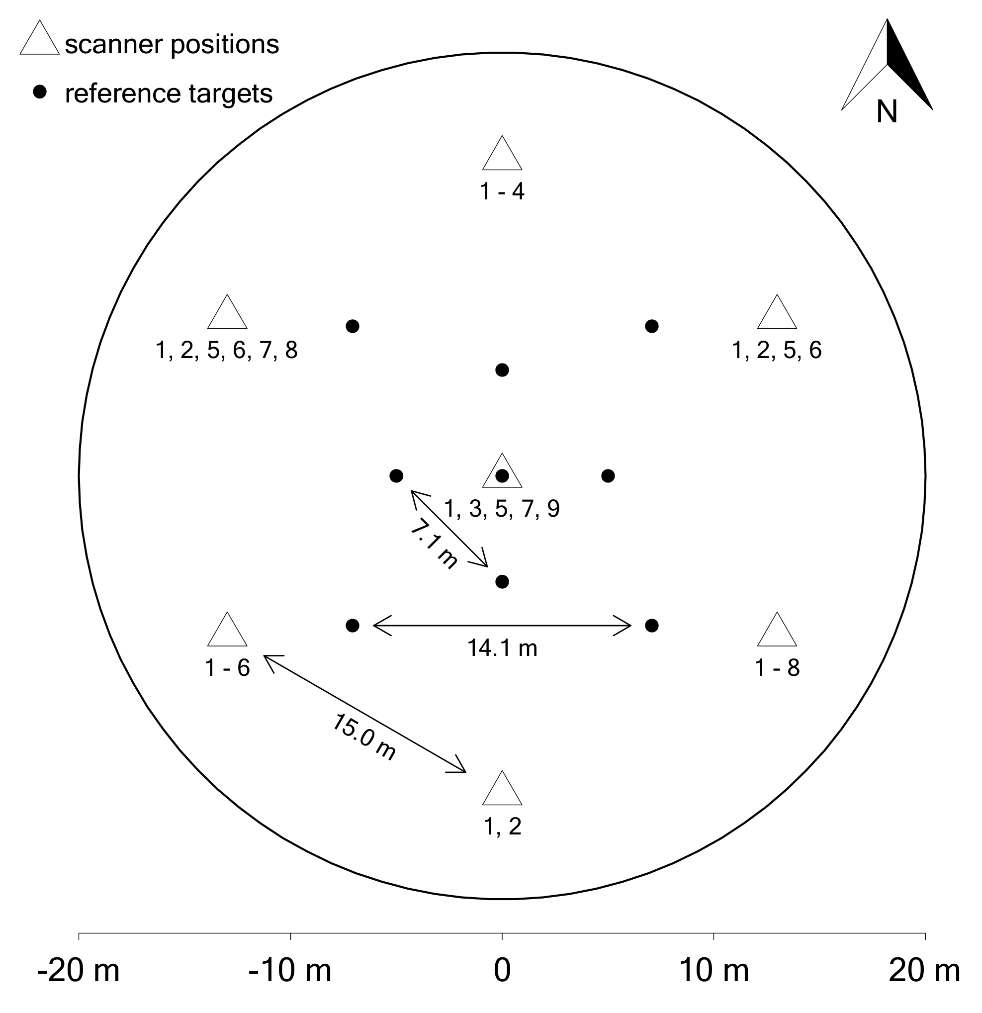
2.2. Instrumentation and Data Collection

Twenty-three sample plots were scanned in February–March 2018 using a FARO Focus3D X330 terrestrial laser scanner (Faro Technologies Inc., Lake Mary, FL, USA). This scanner uses phase-shift light detection and ranging (LIDAR) technology to measure the XYZ positions of objects. The maximum range of the scanner is 330 m and it can measure 9.76 $\times$ 10⁵ points per second. The distances are measured with a continuous wavelength of 1550 nm and an accuracy of ± 2 mm at 10 m distance. The field of view is 360° $\times$ 300°. With a battery capacity of approximately 4.5 h, a weight of 5.2 kg, and a compact design (240 mm $\times$ 200 mm $\times$ 100 mm), the scanner is easy to handle in forestry measurement campaigns. The scan quality parameter was set to 4$\times$, resulting in moderate noise reduction. The quality parameters 1$\times$ through 4$\times$ are different expressions for the observation time: 1$\times$ has the smallest observation time of 1 µs per scan point, and 4$\times$ has 8 µs per scan point. The resolution was set to r = 6.136 mm/10 m, which is 1/4 of the maximum possible resolution (r_max = 1.534 mm/10 m). Furthermore, the hardware settings “Clear Sky” and “Clear Contour” were used to filter incorrect scan points. These settings resulted in a pure scanning time plus photographs of about 11 minutes per scan, and it took approximately 3 minutes more to set up the scanner at a different position, as is necessary in multiscan mode.

A set of nine scan variants was applied, differing in the position of the scanner and the number of scans per plot (see

Table 2. Overview of scan variants with respect to geometric setup, number of scans, and necessary working time.

Variant	Setting	# Of Scans	Scan Time (min)	Approx. Scanner Installation Time (min)	Approx. Sphere Installation Time (min)	Approx. Total Working Time Per Plot (min)
1	Hexagon with center	7	77	21	5	103
2	Hexagon without center	6	66	18	5	89
3	Triangle with center	4	44	12	5	61
4	Triangle without center	3	33	9	5	47
5	Rectangle with center	5	55	15	5	75
6	Rectangle without center	4	44	12	5	61
7	Diagonal with center	3	33	9	5	47
8	Diagonal without center	2	22	6	5	33
9	Single scan (only center)	1	11	3	0	14

). The most intensive scan, variant 1, comprised seven scanner installations, among them six positions arranged in a regular hexagon with a constant edge length of 15 m and centered at the sample point location, plus an additional location positioned at the sample point. Scan variant 9 had the lowest intensity and was the single scan mode, in which the scanner was placed only at the sample plot center. The other seven scan variants were constituted as subsets of the full scan, variant 1, comprising a hexagon without a central scan (variant 2) and other geometrical arrangements in the form of a triangle, a rectangle, and a diagonal, each of which was applied in two subvariants, either including or excluding an additional central scan position.

Figure 1 shows the spatial arrangement of the scanner positions and reference spheres on a sample plot with a 20 m radius. For the most intensive scan, variant 1, the distance between each neighboring scanner position was constantly 15 m. However, if a scanner position was closer than 0.5 m to the nearest tree, it was allowed to be relocated by a maximum distance of 0.5 m in an appropriate direction. To enable easy co-registration of the individual scans, eight Styrofoam balls with a diameter of 150 mm and an additional ball with a diameter of 300 mm mounted on monopods were installed as reference targets on each sample plot. Two sets of the reference targets, each containing four targets, were arranged in regular squares with side lengths of 14.1 m and 7.1 m. That is, the target points of the inner rectangle were 5 m from the sample point, and those of the outer rectangle were 10 m from the sample point (see Figure 1). Once the center scan was completed, the plot center was marked with the reference target ball with a diameter of 300 mm.

2.3. Point Cloud Processing

Co-registration of the raw scan data was performed separately for each scan variant and by means of the Styrofoam reference targets using the FARO SCENE 6.2 program [68]. A constant cutoff distance of 30 m was chosen for each of the seven scanner positions. The aligned scans were then further processed to obtain a complete 3D point cloud for each plot and scan variant containing X, Y, and Z coordinates. These point clouds were then clipped with an upright-oriented cylinder with a radius of 21 m and centered at the sample point. For processing of the point clouds in the subsequent steps, the LAStools software package (rapidlasso GmbH, Gilching, Germany) [69] was used. The point clouds were split into square tiles with an edge length of 10 m plus an additional buffer of 2 m width on each side. Each tile was then processed with the LAStools “lasnoise” noise filter. Subsequently, all points were classified into ground and non-ground points, using a modified version of the algorithm by Axelsson [70], which is implemented in LAStools as “lasground”. The non-ground points were normalized relative to the ground-derived digital elevation model (DEM), and the ground points were discarded from the data. After noise reduction and ground classification, the tiles were reassembled to form a single point cloud for each sample plot. The resulting point cloud data were exported in a tab-delimited text file format. Further data analysis was performed using R statistical software (R Foundation for Statistical Computing, Vienna, Austria) [71]. A step-by-step overview of the entire workflow is given in Appendix A,

Table A2. Workflow and applied software functions and parameters. Compared with Ritter et al. [7], the red steps indicate the additional steps and the gray steps indicate the omitted steps. DEM, digital elevation model.

Step No.	Step/Substep			Software	Package/Function		Parameters
1	Co-registration of scans			FARO
2	Export in xyz format			SCENE
3	Import data			LAStools	txt2las
	Coordinate transformation				las2las		rotate_xy reoffset
	Thinning the point cloud				lasthin		keep_every_nth 2
4	Split point cloud into tiles				lastile		tile_size 10 buffer 2
5	Filter				lasnoise		step 0.35 isolation 850
6	Classify points into ground points and nonground points Normalize relative to DEM				lasground		step 1 spike 0.4 bulge 0.5 offset 0.1 replace z
7	Re-merge tiles and remove ground points				lastile		drop_classification 2
	Splitting point cloud into tiles				lastile		tile_size 25 buffer 5
8	Export in txt format				las2txt
9	Import data			R	data.table	fread()
10a	Stage one clustering		Estimate cutoff distance		densityClust	estimateDC()	NeighbourRateLow = 0.005 NeighbourRateHigh = 0.001
10b			Calculate local density			densityClust()	DC = [estimated dc from estimateDc()]
10c			Find cluster centroids			findClusters()	rho = 2 delta = 0.5
11	Filter stage one clusters				various functions in base
12a	Stage two clustering		Estimate cutoff distance		densityClust	estimateDC()	NeighbourRateLow = 0.01 NeighbourRateHigh = 0.02
12b			Calculate local density			densityClust()	DC = [estimated dc from estimateDc()]
12c			Find cluster centroids			findClusters()	rho = 10 delta = 0.5
			Join clusters with a distance of less than 50 cm		spatstat	connected.ppp()	R = 0.5
13	Diameter estimation	dbh in 13 vertical layers			edci	circMclust()	nx = 25 ny = 25 nr = 5
					conicfit	LMcircleFit
						EllipseDirectFit
		Upper diameter			edci	circMclust()	nx = 25 ny = 25 nr = 5
					conicfit	LMcircleFit
						EllipseDirectFit
14	Check criteria for diameters				various functions in base
15	Assign tree locations		Assign points		spatstat	pppdist()	cutoff = 0.8

.

2.4. Clustering, Detection of Tree Positions, and dbh Measurement

Automatic detection of stem positions and automatic measurement of dbh were carried out using a methodology demonstrated by Ritter et al. [7] that was further refined during the present study. The workflow as well as the changes and innovations compared with Ritter et al. [7] are shown in Table A2. The fundamental principle of the automatic tree detection approach is a density-based clustering algorithm proposed by Rodriguez and Laio [72] that is implemented in the R-package densityClust [73]. The clustering algorithm is solely based on the Euclidean distance between data points. Cluster centroids are defined by local density maxima. The clustering algorithm is based on the rationale that cluster centers (i) are surrounded by areas of lower local density and (ii) are at a relatively large distance from other local density maxima [72]. For each data point $i$, the local density ${\rho }_i$ and distance ${\delta }_i$ from points of higher density are calculated, depending on the distances between data points and a constant cutoff distance $d_c$.

Our stem detection algorithm uses such a density-based clustering in two subsequent phases. In the first clustering phase, the 3D point cloud of normalized Z values was stratified into vertical layers, each of which had a height of 21 cm and a vertical overlap of 20 cm with the layer lying above. The lower border of the lowest layer was placed 1 m above the normalized zero height and the upper border of the topmost layer at a height of 2.88 m. This procedure resulted in 168 vertical layers. From each of these layers, 20,000 points were randomly sampled, and if a layer contained fewer than 20,000 points, the whole point set was selected. Layers with fewer than 500 points were excluded from cluster analysis. The density-based clustering was separately applied to the points selected from each layer.

In the second clustering phase, the cluster centroids from the first phase were additionally clustered. For that purpose, the cluster centroids from the first phase were projected onto a plane by simply dropping their Z-coordinates. Subsequently, the phase-1 cluster centroids were filtered so that the remaining set contained only points with at least 15 neighbors at a 5 cm distance. This filtering caused noise reduction and discarded first-phase centroids that represented branches or regeneration. The filtered phase-1 centroids were then subjected to the phase-2 clustering, which resulted in preliminary estimates of the existing tree positions.

The XY-coordinate range of all points contributing to the phase-2 cluster was used to construct a clipping window around every preliminary tree position estimate. The original 3D point cloud was then clipped accordingly and stratified into 13 vertical layers, each of which had a vertical extent of 15 cm. The lower boundary of the lowest layer was placed at a 1 m height above ground, and the lower boundary of the topmost layer was at a 2.5 m height. The distance between two neighboring layers was 12.5 cm, resulting in a 2.5 cm overlap of neighboring layers. The 3D points from each layer were projected onto the horizontal plane, creating 2-dimensional XY points. Subsequently, circles were separately fitted to the points of each layer using the circular cluster method of Muller and Garlipp [74]. The method was implemented in the R package edci [75]. A regular grid of 25 $\times$ 25 starting points with a mesh width of 3.2 cm was chosen as initial circle centers for the optimization. In addition, a sequence of five starting radii beginning at 1 cm, ending at 50 cm, and with a step width of 9.8 cm was chosen at each grid point. This procedure resulted in 3125 starting values for each of the 13 layers. After accomplishing the circle fit in each vertical layer, annulus-shaped buffer zones were constructed around the circle arcs. Each buffer annulus had a width of 20% of the respective circle radius and an outer radius of 110% of the circle radius. The proportion of points falling into this buffer zone was calculated in relation to the total number of points associated with each layer. The decision as to whether a tree position was finally proposed at a phase-2 cluster centroid location was determined by the results from the circle fits. Trials revealed that the decision could be safely made depending on the following three criteria: for 6 out of the total 13 layers, (i) the circles’ buffer zones should include at least a 55% proportion of the total amount of clipped points, (ii) the standard deviation of the XY position coordinates must be less than or equal to 0.02 m, and (iii) the standard deviation of the diameter measurements must be less than or equal to 1.5 cm. The preliminary proposal of a tree location was rejected if at least one of the three criteria was not met for any of the 1716 total possible combinations of 6 samples from the 13 layers. If several combinations met the three criteria, the one with the highest average number of points in the buffer zone across the six layers was further analyzed to derive the final tree position and dbh measurement. For measurement of the final dbh, it proved to be appropriate to choose the layer closest to the 1.3 m height. However, if a circle fit for a layer around the 1.3 m height was not included by the collective of the six selected layers, the layer closest to the 1.3 m height was successively chosen and the diameter measurement for this layer was corrected by a positive/negative offset of $\pm$1.34 cm m^–1 per deviation from the 1.3 m height. The center of the respective fitted circle was then chosen as the final tree position.

2.5. Reference Data

Reference data for the actual dbh values and tree positions were derived from a combination of field data and manual measurements in the co-registered 3D point clouds. For trees that were included by the Bitterlich relascope sampling, the tree positions and dbh values from the field measurement data served as reference data. For trees that were located within a range of 20 m from the sample point, but were excluded by the Bitterlich sampling, the reference locations and dbh were measured manually within the point cloud using FARO SCENE 6.2 [68]. Because measurement errors could occur with both methods, either the automatic routines or the manual measurements in the field and within the point cloud, it was not guaranteed that the estimated reference position coordinates would be equal to their counterparts in the reference data for any given tree. Thus, a reliable assignment of estimated tree positions to corresponding reference coordinates was required. This assignment was automatically performed using the function pppdist() from the R-package spatstat [76]. This function performs a mapping of two similar point patterns by minimizing the average Euclidean distance between matching points. Automatically detected tree positions that could not be assigned to a tree measured in the reference data were manually double-checked in the TLS point cloud. Depending on the results of the check, either the automatically detected tree position was marked as a false positive, or if the tree was visible in the point cloud, but simply missed during the reference measurements in the field, the coordinates were added post hoc to the reference data.

2.6. Test by Means of Independent Reference Data from an International Benchmark Project

To test the performance of our algorithms by means of other independent reference data, our methodology was also applied to the publicly available TLS dataset, comprising six sample plots that were collected for an international TLS benchmarking project [6] in Evo, Finland. Eighteen partners from Asia, Europe, and North America participated in the project and submitted their retrieved tree attributes for evaluation. Out of a total of 18 participants, 15 partners provided results achieved with their own algorithms for tree detection and dbh measurement.

The TLS data of the benchmarking project was collected on 24 sample plots with different characteristics (categories), and 6 of them including reference field data have been made publicly available for nonprofit research purposes. The “easy” category represents sample plots that had clear stem visibility with minimal understory vegetation and low stem density, the “medium” category represents sample plots with moderate stem density and sparse understory vegetation, and the “difficult” category represents sample plots that had high stem density and dense understory vegetation. All scans were carried out in both single and multiple scan modes. The reader is referred to the original work by Liang et al. [6] for further details.

2.7. Accuracy of Tree Detection and dbh Measurement

The accuracy of tree detection was evaluated in terms of three measures: detection rate $d_r\left(\%\right)$, commission error $c\left(\%\right)$, and overall accuracy $acc\left(\%\right)$. These measures were calculated as follows:

$$d_r\left(\%\right)=\frac{n_{\mathrm{match}}}{n_{\mathrm{ref}}}\times 100,$$

(1)

$$c\left(\%\right)=\frac{n_{\mathrm{falsepos}}}{n_{\mathrm{extr}}}\times 100,$$

(2)

$$acc\left(\%\right)=100\%-\left(o\left(\%\right)+c\left(\%\right)\right),$$

(3)

where $n_{\mathrm{match}}$ is the number of correctly found reference trees; $n_{\mathrm{ref}}$ is the total number of reference trees; $n_{\mathrm{falsepos}}$ is the number of tree positions, which could not be assigned to an existing tree in the reference data; $n_{\mathrm{extr}}$ is the number of automatically detected tree positions ($n_{\mathrm{match}}+n_{\mathrm{falsepos}}$); and $o\left(\%\right)$ is the omission error, defined as $100\%-d_r\left(\%\right)$. The detection rate $d_r\left(\%\right)$ measures the proportion of correctly detected tree locations. The commission error $c\left(\%\right)$ measures the proportion of falsely detected tree locations. The overall accuracy $acc\left(\%\right)$ is a combination of the latter two metrics and represents a global quality criterion.

The precision of the automatic dbh measurements was assessed by means of root mean square error (RMSE) calculated as the square root of the average quadratic distance between the automatic measurement ${\widehat{dbh}}_i$ and the corresponding reference measurement $db{h}_i$.

$$RMSE=\sqrt{\frac{1}{n_{\mathrm{match}}}{{\displaystyle \sum }}_{i=1}^{n_{\mathrm{match}}}{\left({\widehat{dbh}}_i-db{h}_i\right)}^2}$$

(4)

The accuracy of the automatic dbh measurements was assessed in terms of bias:

$$bias=\frac{1}{n_{\mathrm{match}}}{{\displaystyle \sum }}_{i=1}^{n_{\mathrm{match}}}\left({\widehat{dbh}}_i-db{h}_i\right).$$

(5)

The latter two criteria were also calculated as relative measures, as percentage RMSE% and percentage bias%:

$$RMSE\%=\frac{RMSE}{\overline{dbh}}\times 100,$$

(6)

$$bias\%=\frac{bias}{\overline{dbh}}\times 100,$$

(7)

with

$$\overline{dbh}=\frac{1}{n_{match}}{{\displaystyle \sum }}_{i=1}^{n_{match}}db{h}_i$$

(8)

being the average dbh of the reference data.

In order to examine whether and to what extent the accuracy of the automatic tree detection and the accuracy and precision of the dbh measurements were influenced by the distance of a tree to the sample plot center, the performance measures described above were separately assessed for four subplot sizes defined by disks with radii of 20 m, 15 m, 10 m, and 5 m. In addition, whether the performance of the automatic routines showed trends depending on the size of the trees was also analyzed. For this purpose, the performance measures were evaluated for subsets defined by three lower dbh thresholds of 5 cm, 10 cm, and 15 cm. Finally, the nine scan variants were ranked with respect to (i) the associated labor costs, (ii) the overall accuracy on average achieved with the different sample plot radii and dbh thresholds, and (iii) the average RMSE.

As it turned out that scan variant 3 would provide a good compromise between performance and labor costs, its performance was analyzed in depth with respect to the influence of an applied maximum radius (plot size) and the effects of stand characteristics and topographic measures. To evaluate the significant effects of the above-mentioned covariates, we tested the relationship between detection rate/commission error and the stand and terrain characteristics given in Table 1. A logistic regression model was formulated using the glm() function in R. As the detection and commission rate are proportional data, a quasibinomial logit model has been fitted. Before that, the predictor variables were plotted against the dependent variable and in the course of modeling, and any plausible interactions were also tested. As interpreting the model parameters is difficult because of multicollinearity problems, the number of predictor variables was reduced with the support of correlation coefficients. Finally, the saturated model for the logistic regression was formulated as follows:

$$y=\frac{\exp \left(\eta \right)}{1+\exp \left(\eta \right)},$$

(9)

with

$$\begin{gathered} \eta ={\beta }_0+{\beta }_1\times slope+{\beta }_2\times dm+{\beta }_3\times N/ha+{\beta }_4\times CVdbh, \\ +{\beta }_5\times CE+{\beta }_6\times Shannon+{\beta }_7\times p_{dec}+ϵ, \end{gathered}$$

(10)

where $y$ is either the detection rate or the commission error between 0 and 1, $\eta$ is a linear predictor, and ${\beta }_0,\dots ,{\beta }_7$ are linear coefficients.

A backward selection of predictor variables was applied to these full models, resulting in models from which Efron’s pseudo coefficient of determination [77] was calculated.

3. Results

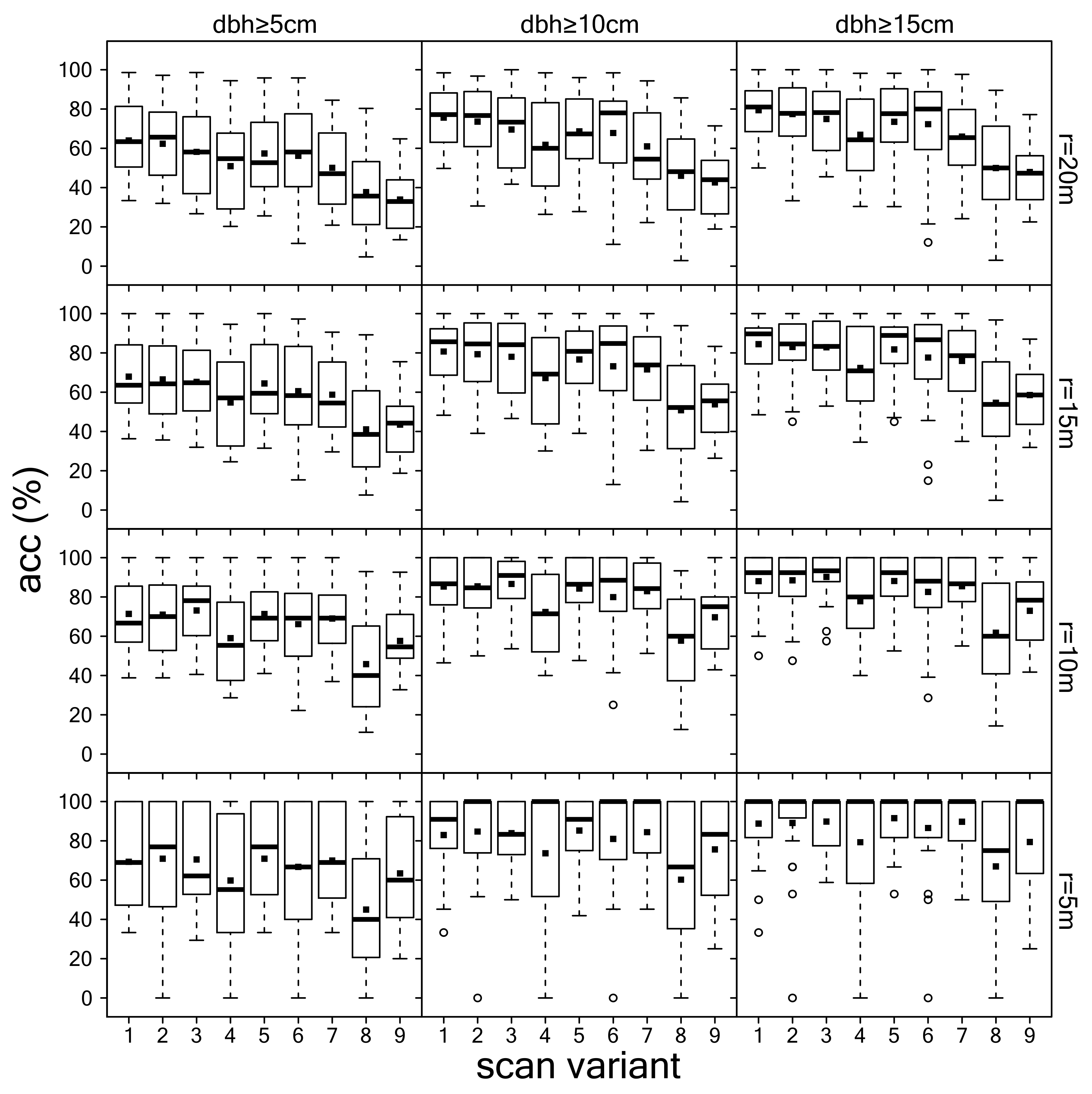
3.1. Detection of Tree Positions

The analysis of the 23 plots showed that the detection rate $d_r\left(\%\right)$ over all scan variants strongly depended on the lower dbh threshold and the sample plot radius applied as a maximum radius (Figure 2). In general, the detection rate increased with an increasing lower threshold for dbh and a decreasing maximum radius. Furthermore, it can be seen that scan variants with fewer scans generally have lower detection rates. Scan variants without a scan position at the sample plot center (2, hexagon; 4, triangle; 6, rectangle; 8, diagonal) showed lower detection rates than their counterparts that included a central scan position (1, hexagon; 3, triangle; 5, rectangle; 7, diagonal). This difference between scan variants with and without a central scan position was greater with a smaller number of scans. This means that the difference is smallest between scan variants 1 and 2 (7 and 6 scanner positions, respectively) and largest between variants 7 and 8 (3 and 2 scanner positions, respectively). Under plot radii of 15 m, 10 m, and 5 m, single scan variant 9 showed higher detection rates than variant 8 (diagonal without center). The average detection rates over all 23 sample plots and across all scan variants, dbh thresholds, and plot radii ranged from 34.4% to 92% (see further details in Appendix A,

Table A3. Detection rates for different scan variants, lower dbh thresholds, and plot radii.

		$$\begin{gathered} \mathbf{Scan}\mathbf{Variants} \\ \mathbf{Detection}\mathbf{Rate}{\mathit{d}}_{\mathit{r}}\left(\mathit{\%}\right) \end{gathered}$$
Radius	dbh	1	2	3	4	5	6	7	8	9
20 m	≥5 cm	65.31	63.59	59.09	51.47	58.29	57.12	50.62	38.43	34.36
20 m	≥10 cm	77.57	75.47	70.82	62.71	69.98	69.09	61.76	46.93	43.09
20 m	≥15 cm	82.39	80.25	76.73	68.25	75.46	74.06	67.09	51.19	48.53
15 m	≥5 cm	68.80	67.25	66.17	55.26	65.13	61.22	59.38	41.89	44.31
15 m	≥10 cm	82.10	80.47	79.22	67.93	77.67	74.17	72.48	51.88	54.68
15 m	≥15 cm	86.54	84.75	84.50	73.51	83.31	78.92	77.11	55.91	59.49
10 m	≥5 cm	72.54	71.79	74.30	59.38	72.21	66.60	69.47	45.93	58.57
10 m	≥10 cm	87.19	86.81	88.16	73.08	85.72	80.66	83.68	58.06	70.68
10 m	≥15 cm	90.46	90.18	92.04	78.78	89.97	83.55	86.66	62.10	74.06
5 m	≥5 cm	69.33	70.89	70.52	59.91	70.93	66.81	69.94	45.00	63.41
5 m	≥10 cm	82.93	84.72	83.93	73.80	85.23	81.09	84.4	60.22	75.63
5 m	≥15 cm	88.75	89.11	89.80	79.55	91.50	86.79	89.69	66.96	79.40

).

In comparison with the omission error ($100\%-d_r\left(\%\right))$, the commission error ($c\left(\%\right)$ ) was less relevant (see Figure 3). However, the commission error was likewise dependent on the settings and increased with increasing lower dbh threshold and maximum radius. The commission error differed only slightly among scan variants, especially for lower plot sizes. However, single scan variant 9 mostly resulted in lower commission errors. The average commission error over all 23 sample plots and depending on scan variant, dbh threshold, and plot radius ranged from 0% to 3.8% (see Appendix A,

Table A4. Commission errors for different scan variants, lower dbh thresholds, and plot radii.

		$$\begin{gathered} \mathbf{Scan}\mathbf{Variants} \\ \mathbf{Commission}\mathbf{Error}\mathit{c}\left(\mathit{\%}\right) \end{gathered}$$
Radius	dbh	1	2	3	4	5	6	7	8	9
20 m	≥5 cm	2.16	2.32	1.77	1.55	1.89	2.32	1.53	2.59	0.87
20 m	≥10 cm	2.63	2.82	2.03	1.82	2.19	2.64	1.73	2.91	0.91
20 m	≥15 cm	3.62	3.75	2.57	2.36	2.82	3.14	2.17	3.25	1.08
15 m	≥5 cm	1.37	1.18	1.37	1.27	1.06	1.56	1.31	2.32	1.00
15 m	≥10 cm	1.66	1.43	1.57	1.49	1.27	1.83	1.51	2.66	1.05
15 m	≥15 cm	2.38	2.03	1.96	1.87	1.73	2.12	1.84	2.80	1.15
10 m	≥5 cm	1.69	1.26	1.50	1.01	1.25	0.77	0.81	0.43	1.00
10 m	≥10 cm	2.01	1.48	1.66	1.19	1.51	0.90	1.01	0.52	1.07
10 m	≥15 cm	2.50	1.80	1.87	1.42	1.93	1.18	1.42	0.55	1.18
5 m	≥5 cm	0	0	0	0.27	0	0.23	0	0	0
5 m	≥10 cm	0	0	0	0.30	0	0.28	0	0	0
5 m	≥15 cm	0	0	0	0.45	0	0.41	0	0	0

for further details).

Overall accuracy rates ($acc\left(\%\right)$), as a combination of detection and commission rates, are presented in Figure 4. Overall accuracy showed similar behavior to the detection rate depending on dbh threshold, plot radius, and scan variant. Average overall accuracies across all sample plots were between 33.9% and 90.2% (details are provided in Appendix A,

Table A5. Overall accuracies for different scan variants, lower dbh thresholds, and plot radii.

		Scan Variants Overall Accuracy acc(%)
Radius	dbh	1	2	3	4	5	6	7	8	9
20 m	≥5 cm	64.00	62.32	58.19	50.89	57.37	56.18	50.08	37.72	33.92
20 m	≥10 cm	75.59	73.57	69.56	61.80	68.66	67.80	61.00	45.99	42.60
20 m	≥15 cm	79.42	77.40	74.91	66.87	73.53	72.29	65.95	49.99	47.94
15 m	≥5 cm	67.94	66.53	65.30	54.78	64.46	60.54	58.76	41.07	43.53
15 m	≥10 cm	80.73	79.33	78.07	67.19	76.66	73.23	71.63	50.84	53.83
15 m	≥15 cm	84.46	83.03	82.90	72.36	81.82	77.66	75.93	54.66	58.58
10 m	≥5 cm	71.36	70.94	73.06	58.96	71.28	66.10	68.97	45.74	57.55
10 m	≥10 cm	85.25	85.39	86.59	72.33	84.28	79.88	82.89	57.74	69.60
10 m	≥15 cm	88.00	88.43	90.18	77.78	88.07	82.51	85.46	61.75	72.90
5 m	≥5 cm	69.33	70.89	70.52	59.81	70.93	66.71	69.94	45.00	63.41
5 m	≥10 cm	82.93	84.72	83.93	73.65	85.23	80.95	84.40	60.22	75.63
5 m	≥15 cm	88.75	89.11	89.80	79.30	91.50	86.53	89.69	66.96	79.40

).

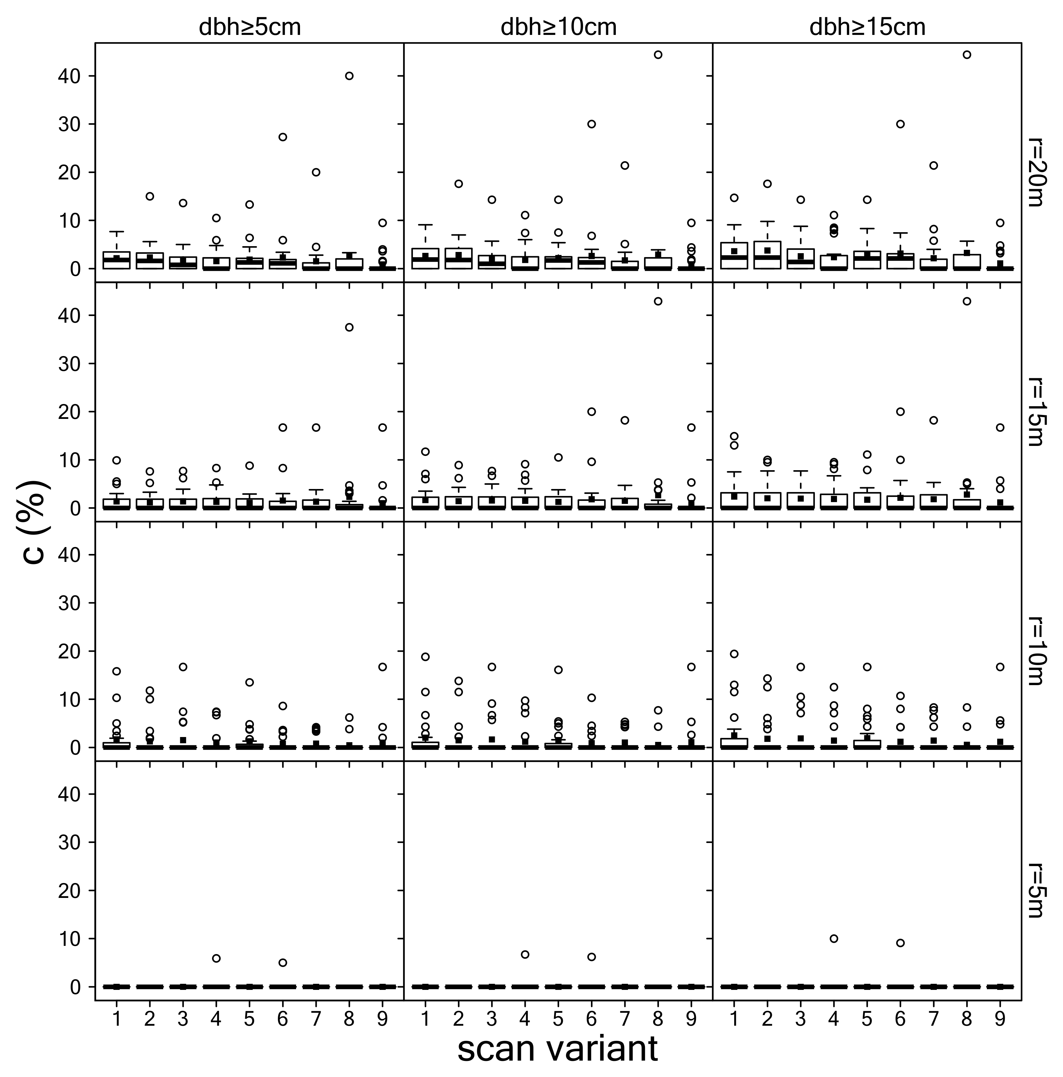
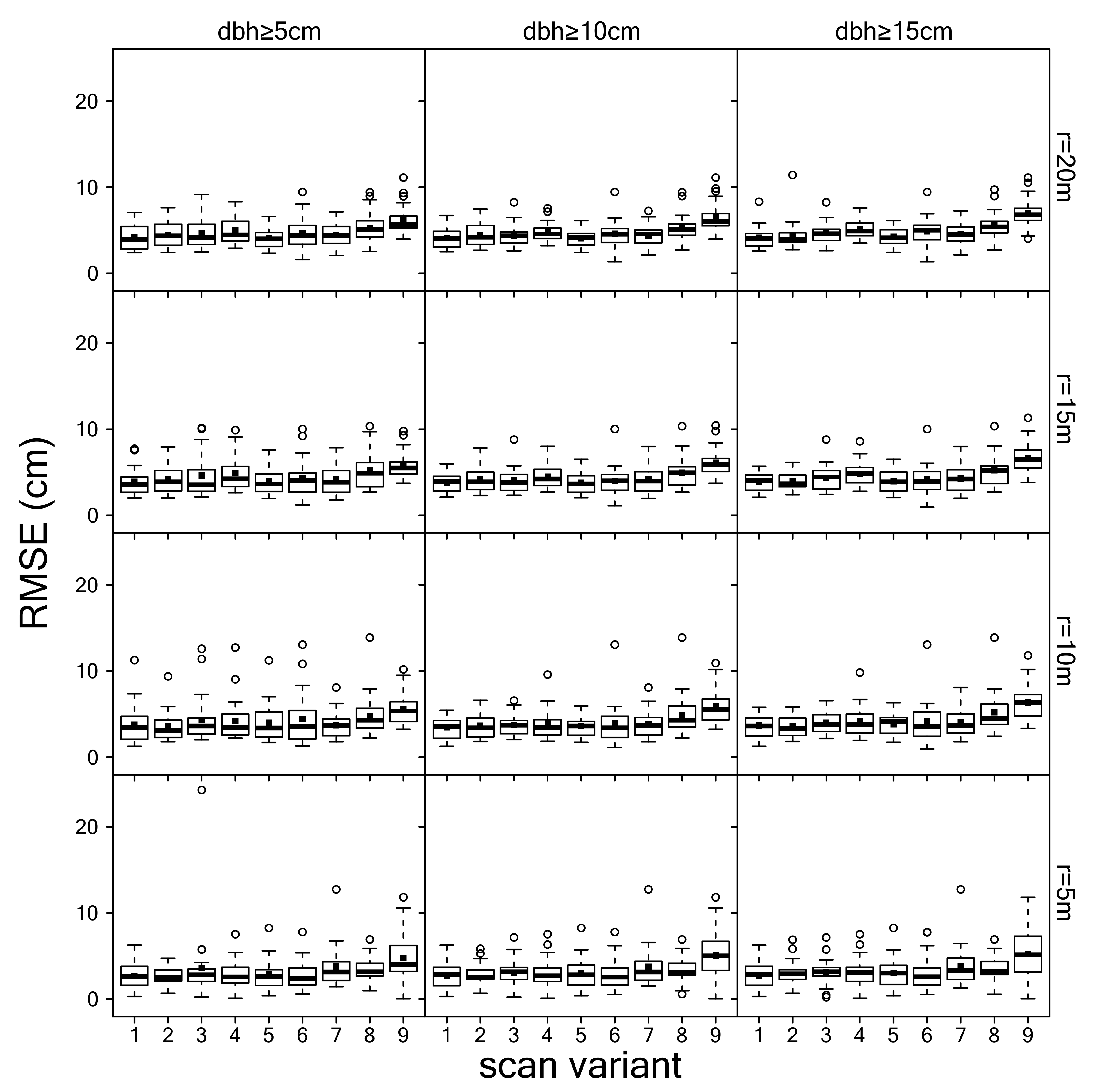
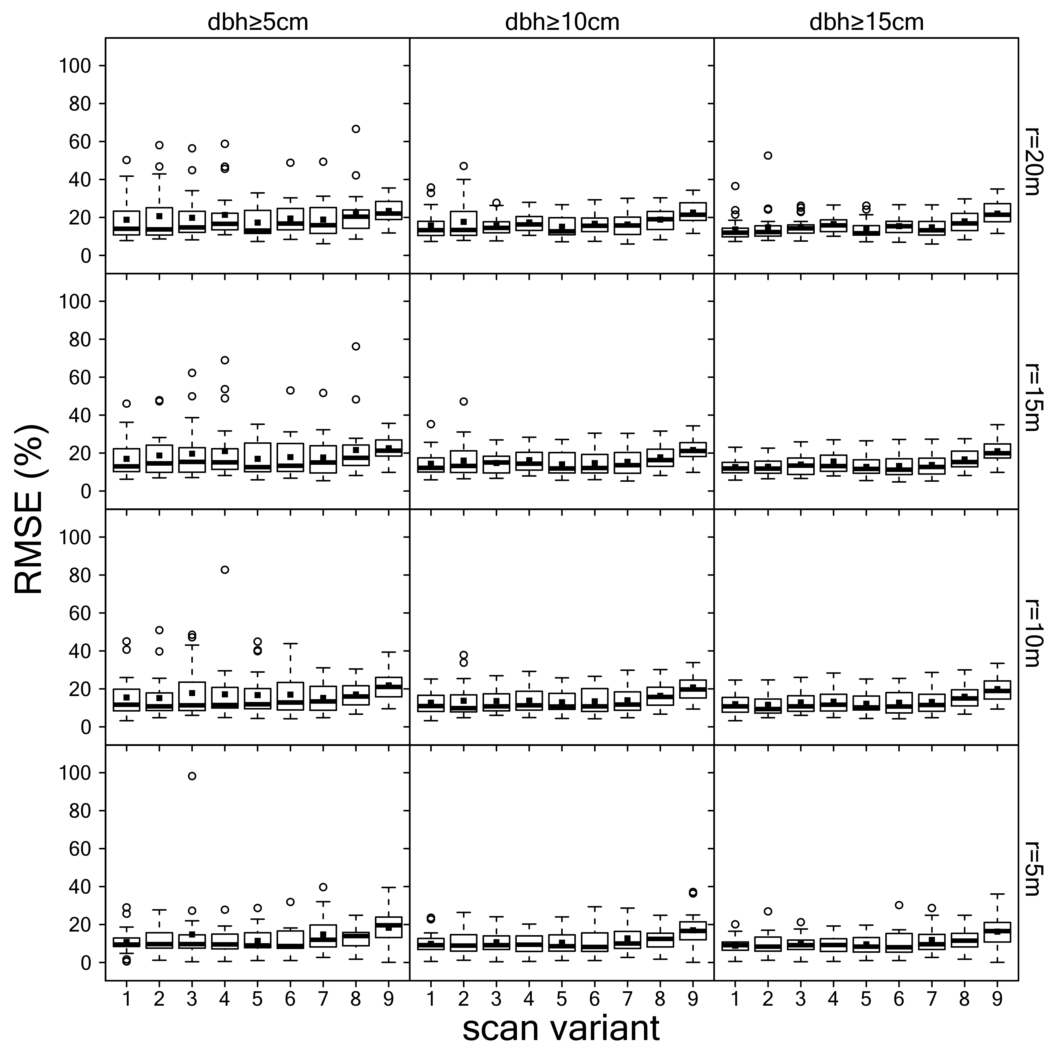
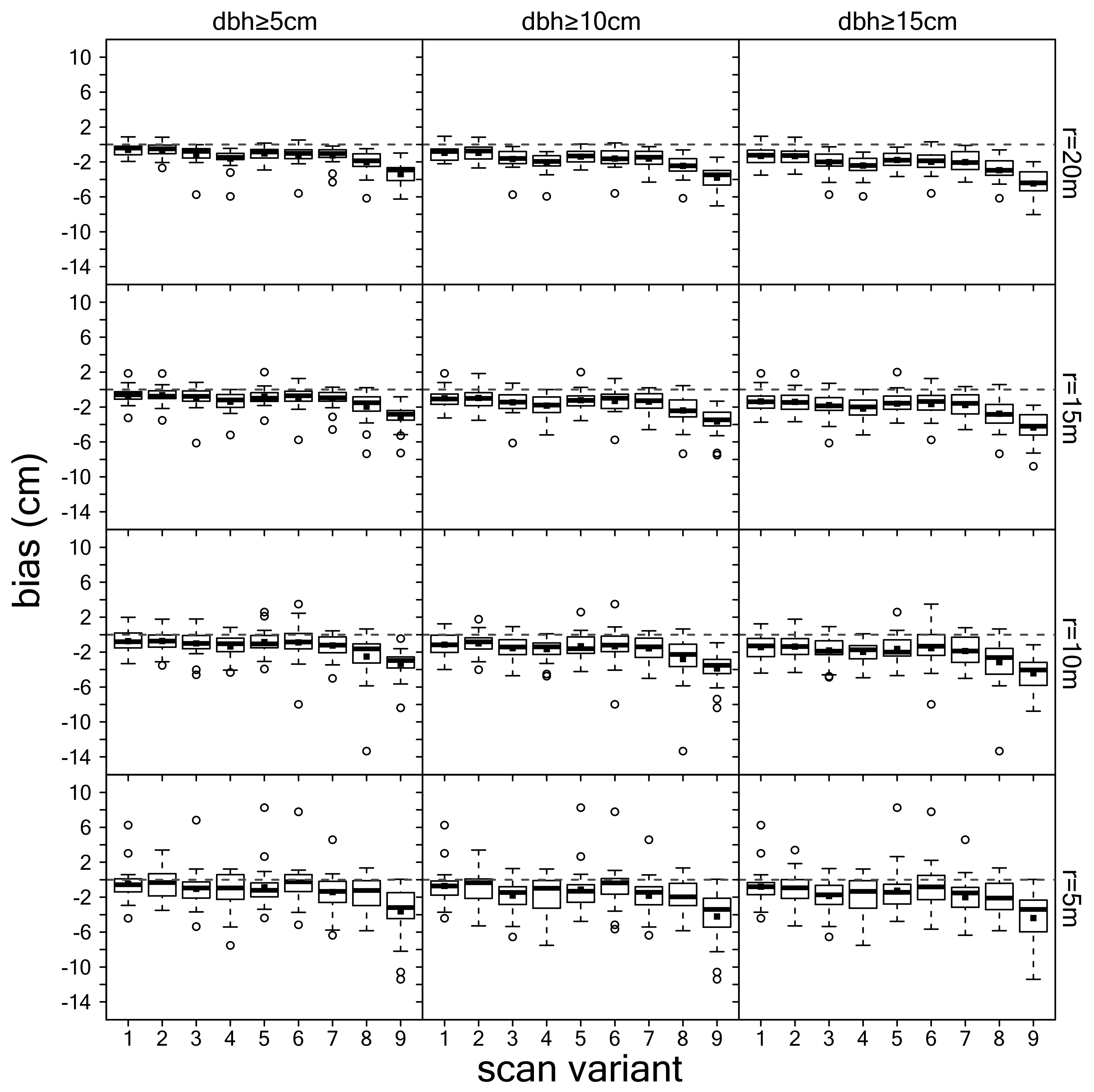
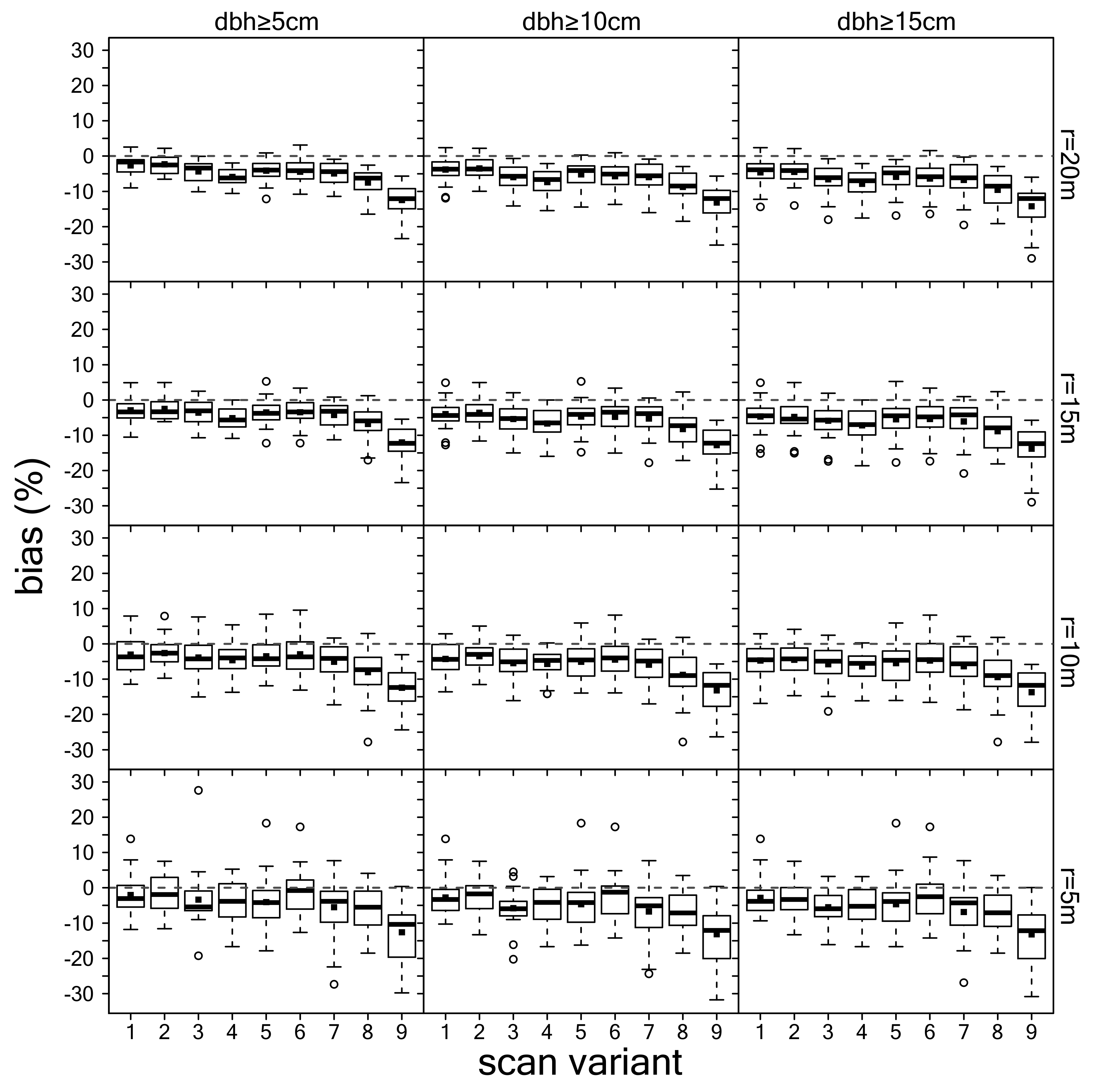
3.2. Estimation of dbh

The performance of the automatic dbh estimation is outlined in

Table 3. Average root mean square error (RMSE) of automatic dbh measurements over all 23 sample plots and depending on scan variant, lower dbh threshold, and plot radius.

		Scan Variants RMSE in cm (RMSE in %)
Radius	dbh	1	2	3	4	5	6	7	8	9
20 m	≥5 cm	4.18 (18.78)	4.48 (20.69)	4.70 (19.78)	5.06 (21.34)	4.08 (17.29)	4.70 (19.39)	4.48 (18.85)	5.29 (22.04)	6.24 (23.43)
20 m	≥10 cm	4.09 (15.83)	4.48 (17.69)	4.34 (15.74)	4.79 (17.35)	4.05 (15.10)	4.61 (16.69)	4.39 (16.28)	5.20 (18.84)	6.51 (22.59)
20 m	≥15 cm	4.14 (13.66)	4.43 (14.80)	4.66 (14.92)	5.14 (16.54)	4.25 (13.77)	4.87 (15.41)	4.56 (14.77)	5.57 (17.89)	7.00 (22.05)
15 m	≥5 cm	3.92 (16.98)	4.20 (18.76)	4.61 (19.70)	4.92 (21.04)	3.96 (16.98)	4.28 (17.89)	4.21 (17.71)	5.22 (21.62)	5.77 (22.62)
15 m	≥10 cm	3.79 (14.43)	4.15 (16.07)	4.04 (14.79)	4.49 (16.32)	3.78 (14.12)	4.01 (14.69)	4.17 (15.41)	4.95 (17.76)	6.09 (21.64)
15 m	≥15 cm	3.90 (12.65)	3.98 (12.83)	4.35 (13.98)	4.83 (15.58)	3.93 (12.79)	4.15 (13.23)	4.27 (13.78)	5.22 (16.70)	6.65 (21.00)
10 m	≥5 cm	3.76 (15.46)	3.63 (15.14)	4.33 (17.76)	4.22 (17.11)	4.01 (16.70)	4.41 (16.96)	3.72 (15.20)	4.81 (16.99)	5.55 (21.83)
10 m	≥10 cm	3.46 (12.70)	3.65 (13.71)	3.75 (13.58)	3.93 (13.82)	3.60 (12.94)	3.94 (13.40)	3.82 (13.95)	4.91 (16.32)	5.91 (20.69)
10 m	≥15 cm	3.68 (11.89)	3.64 (11.62)	4.01 (12.85)	4.14 (13.25)	3.82 (12.17)	4.17 (12.68)	4.05 (13.06)	5.20 (15.85)	6.36 (19.88)
5 m	≥5 cm	2.66 (10.78)	2.69 (11.10)	3.63 (14.77)	2.93 (10.78)	2.93 (11.41)	2.87 (11.16)	3.78 (14.78)	3.45 (12.81)	4.74 (18.30)
5 m	≥10 cm	2.74 (9.80)	2.85 (10.17)	3.03 (10.64)	2.97 (9.64)	3.04 (10.40)	2.96 (10.02)	3.75 (12.71)	3.43 (11.87)	5.07 (16.97)
5 m	≥15 cm	2.74 (8.85)	3.03 (9.86)	3.12 (9.93)	3.07 (9.35)	3.06 (9.56)	3.09 (9.66)	3.82 (11.84)	3.56 (11.75)	5.22 (16.25)

(RMSE) and

Table 4. Average bias of automatic dbh measurements over all 23 sample plots and depending on scan variant, lower dbh threshold, and plot radius.

		Scan Variants Bias in cm (Bias in %)
Radius	dbh	1	2	3	4	5	6	7	8	9
20 m	≥5 cm	−0.62 (−2.64)	−0.63 (−2.33)	−1.18 (−4.36)	−1.61 (−5.93)	−1.03 (−4.12)	−1.21 (−4.12)	−1.26 (−4.91)	−2.03 (−7.51)	−3.39 (−12.48)
20 m	≥10 cm	−0.95 (−3.82)	−0.95 (−3.51)	−1.66 (−5.98)	−2.05 (−7.37)	−1.39 (−5.19)	−1.61 (−5.69)	−1.61 (−5.97)	−2.45 (−8.72)	−3.81 (−13.17)
20 m	≥15 cm	−1.31 (−4.59)	−1.34 (−4.47)	−2.03 (−6.57)	−2.42 (−7.85)	−1.77 (−5.85)	−1.99 (−6.35)	−2.02 (−6.74)	−2.95 (−9.57)	−4.47 (−14.23)
15 m	≥5 cm	−0.66 (−2.92)	−0.64 (−2.51)	−0.96 (−3.61)	−1.40 (−5.15)	−0.83 (−3.52)	−0.92 (−3.47)	−1.05 (−4.23)	−1.97 (−6.80)	−3.17 (−12.02)
15 m	≥10 cm	−1.01 (−4.00)	−0.96 (−3.61)	−1.47 (−5.40)	−1.83 (−6.67)	−1.22 (−4.70)	−1.31 (−4.77)	−1.37 (−5.25)	−2.39 (−8.24)	−3.66 (−12.80)
15 m	≥15 cm	−1.36 (−4.69)	−1.41 (−4.81)	−1.79 (−5.88)	−2.18 (−7.19)	−1.61 (−5.46)	−1.66 (−5.37)	−1.78 (−6.09)	−2.77 (−8.86)	−4.36 (−13.80)
10 m	≥5 cm	−0.75 (−3.05)	−0.73 (−2.62)	−1.01 (−3.85)	−1.35 (−4.62)	−0.85 (−3.52)	−0.89 (−2.94)	−1.25 (−5.07)	−2.51 (−7.99)	−3.35 (−12.42)
10 m	≥10 cm	−1.15 (−4.28)	−1.00 (−3.48)	−1.54 (−5.47)	−1.65 (−5.69)	−1.34 (−5.07)	−1.33 (−4.45)	−1.57 −5.91)	−2.79 (−8.76)	−3.89 (−13.18)
10 m	≥15 cm	−1.42 (−4.71)	−1.37 (−4.50)	−1.82 (−5.75)	−1.97 (−6.37)	−1.63 (−5.44)	−1.56 (−4.70)	−1.88 (−6.33)	−3.16 (−9.39)	−4.43 (−13.69)
5 m	≥5 cm	−0.46 (−2.06)	−0.52 (−1.77)	−1.04 (−3.35)	−1.34 (−3.73)	−0.86 (−4.06)	−0.38 (−1.14)	−1.42 (−5.51)	−1.58 (−5.56)	−3.63 (−12.60)
5 m	≥10 cm	−0.72 (−2.78)	−0.85 (−2.74)	−1.82 (−5.80)	−1.68 (−4.87)	−1.14 (−4.65)	−0.71 (−2.29)	−1.83 (−6.71)	−1.98 (−6.91)	−4.22 (−13.17)
5 m	≥15 cm	−0.81 (−2.86)	−0.95 (−3.08)	−1.86 (−5.53)	−1.82 (−5.21)	−1.26 (−4.65)	−0.74 (−2.42)	−2.00 (−6.86)	−2.10 (−7.05)	−4.40 (−13.18)

(bias) for the different scan variants, lower dbh thresholds, and plot radii. Boxplots of the data can be found in Appendix A, Figures A1–A4. It turns out that scan variants with fewer scans generally showed a higher RMSE and bias. Single scan variant 9 had the largest RMSE and bias of all scan variants. With an increasing lower dbh threshold, bias increased, whereas RMSE remained nearly constant. With decreasing plot radii, RMSE decreased, while bias remained nearly constant. Scan variants without a center scan (2, hexagon; 4, triangle; 6, rectangle; 8, diagonal) mostly had higher RMSE compared with their complete counterparts that included a central scan position (1, hexagon; 3, triangle; 5, rectangle; 7, diagonal); the differences were especially pronounced between scan variants 7 and 8. With regard to bias, a clear difference existed only between scan variants 7 (diagonal with center) and 8 (diagonal without center) when comparing variants with and without the central scan. Average RMSE over all 23 sample plots and across scan variants, dbh thresholds, and plot radii ranged from 2.7 cm to 7 cm. Average relative RMSE was between 8.9% and 23.4%. Absolute bias ranged from 0.5 cm to 4.5 cm and relative bias from 1.8% to 14.5%.

3.3. Summary Evaluation of Scan Variants

Table 5. Ranking of scan variants.

Scan Variant	Working Time Per Plot (min)	Overall Accuracy (%)	RMSE (cm)	Standardized Working Time Per Plot (0, … , 1)	Standardized Overall Accuracy (0, … , 1)	Standardized RMSE (0, … , 1)	Average Standardized Value	Overall Rank
1	103	78.15	3.59	1.000	0.000	0.000	0.333	6
2	89	77.64	3.77	0.843	0.019	0.077	0.313	5
3	61	76.92	4.05	0.528	0.046	0.197	0.257	1
4	47	66.31	4.21	0.371	0.444	0.265	0.360	7
5	75	76.15	3.71	0.685	0.075	0.051	0.270	3
6	61	72.53	4.00	0.528	0.211	0.175	0.305	4
7	47	72.06	4.08	0.371	0.228	0.209	0.269	2
8	33	51.47	4.74	0.213	1.000	0.491	0.568	8
9	14	58.24	5.93	0.000	0.746	1.000	0.582	9

shows the ranking of individual scan variants with respect to standardized labor costs (in terms of working time), standardized overall accuracy, and standardized RMSE of the dbh measurements. The overall accuracy and RMSE for each scan variant were calculated as average values for the different settings (plot radii and dbh thresholds) based on the figures presented in Table A5 and Table 4. Scan variant 9 (single scan) was associated with the least working time (standardized value of 0), and scan variant 1 (hexagon with center) had the most working time (standardized value of 1) with seven scan positions. The best overall accuracy (78.15%, standardized value of 0) was achieved with variant 1 (hexagon with center) and the worst (51.47%, standardized value of 1) was with variant 8 (diagonal without center). In terms of RMSE, scan variant 1 (hexagon with center) showed the best performance (RMSE of 3.59 cm, standardized value of 0), and scan variant 9 (single scan) had the poorest performance (RMSE of 5.93 cm, standardized value of 1). According to an overall ranking, scan variant 3 could be regarded as superior (lowest standardized value of 0.257), and scan variant 9 showed the worst overall performance (highest standardized value of 0.257). Variant 3 (triangle with center), with a standardized working time of 0.528, a standardized overall accuracy of 0.046, and a standardized precision of automatic dbh measurement of 0.197, represented a good compromise between labor cost and accuracy of automatic stem detection and dbh measurement.

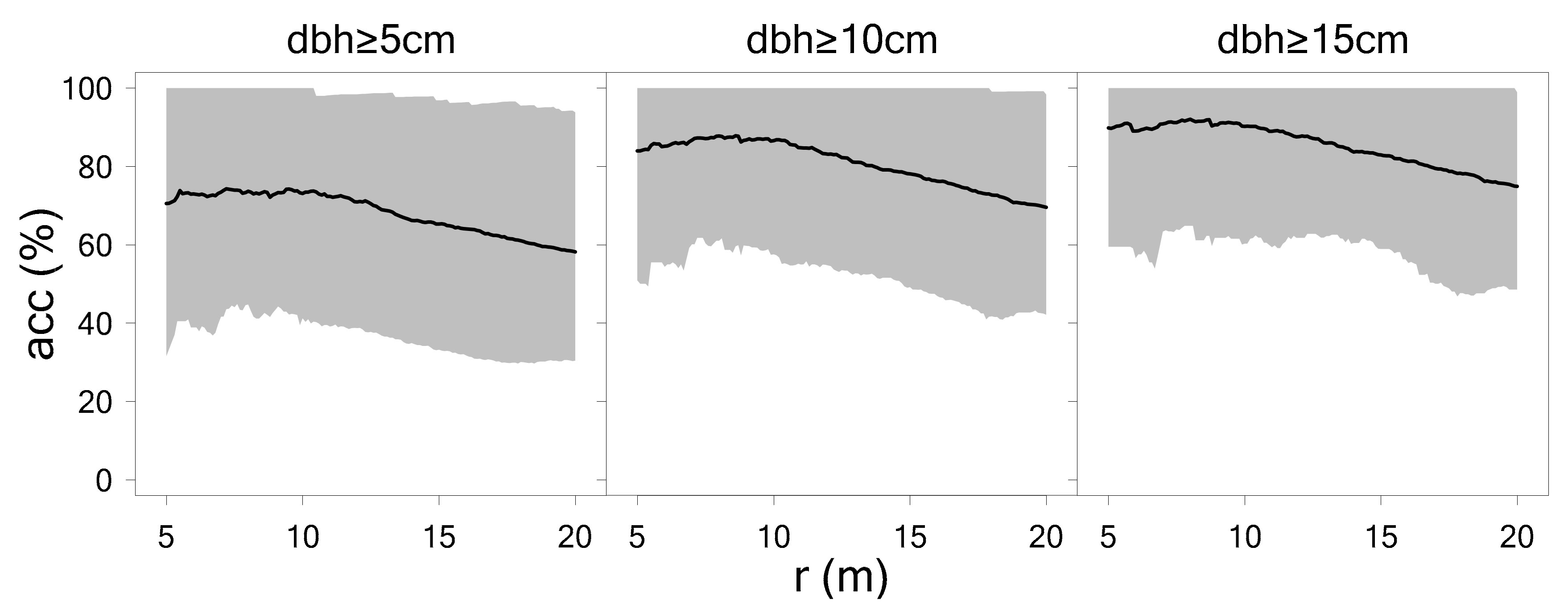
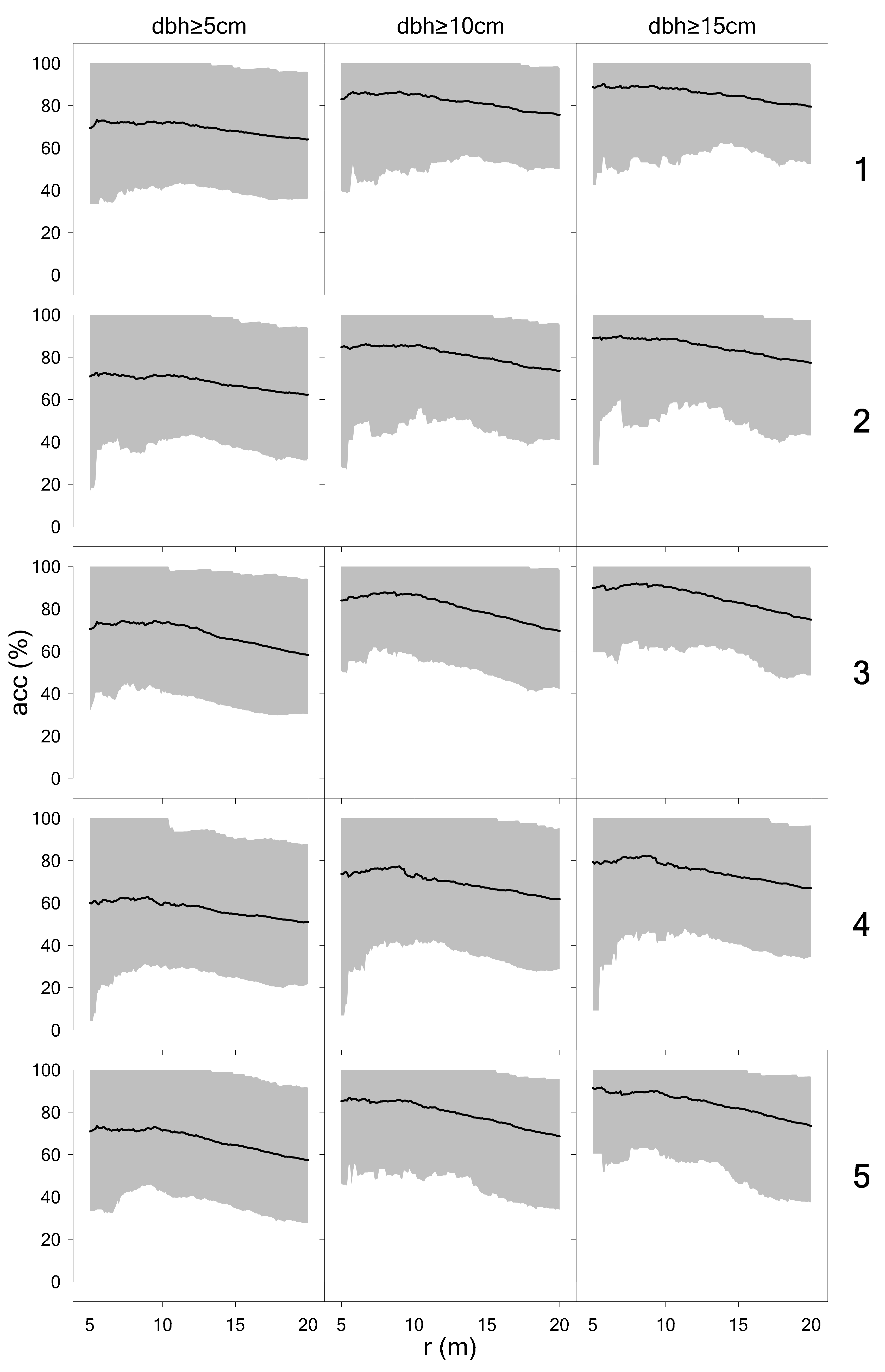
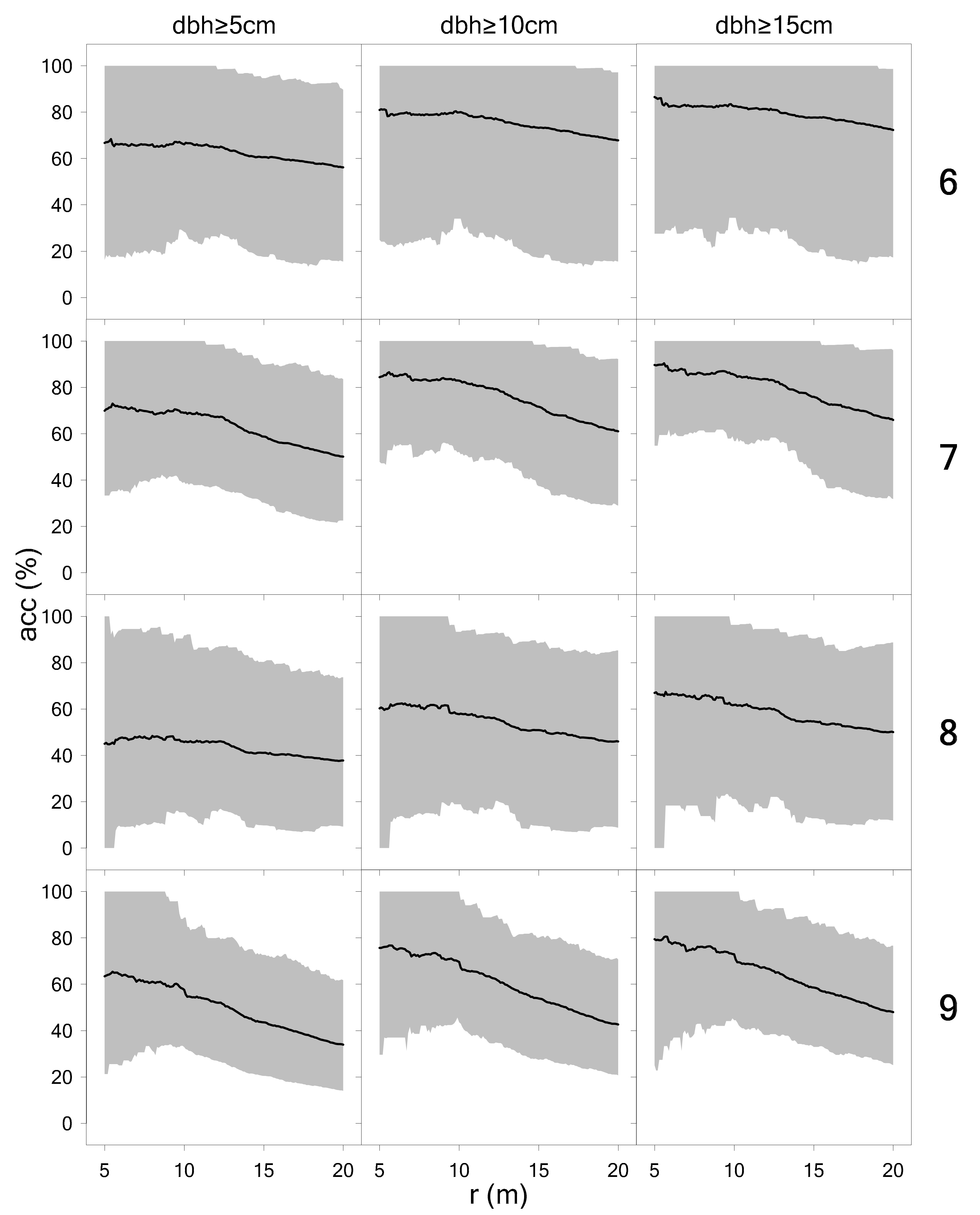
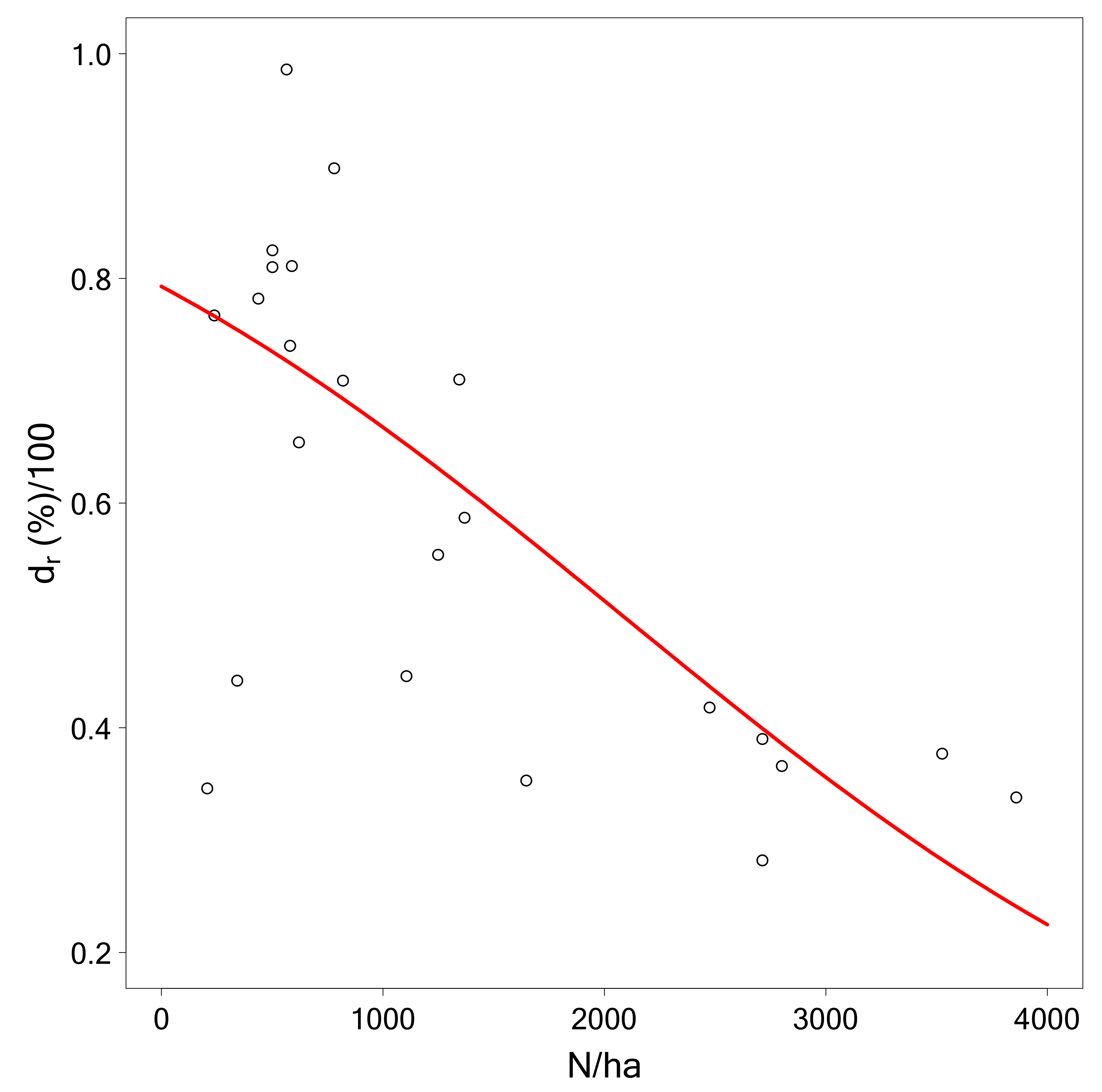
3.4. Relationship to Plot Radius and Environmental Variables

The relationship between overall detection accuracy and maximum radius, that is, sample plot radius, was analyzed in more detail for scan variant 3 (triangle plus central scan). The results are shown in Figure 5. The curves of the accuracy rates had a similar shape for all three lower dbh thresholds. However, the level of the curve, that is, the overall accuracy, was lowest for the 5 cm threshold and highest for the 15 cm threshold. For each of the three applied dbh thresholds, overall accuracy remained almost constant across a range of maximum radii between 5 and 10 m, and overall accuracy continuously declined for maximum radii greater than 10 m. Corresponding graphs for the other scan variants are shown in Appendix A (Figure A5 and Figure A6). Analysis revealed that the curves of scan variants without a central scan position (variants 2, 4, 6, 8) had a flatter trend than the curves of scan variants with a central scan (variants 1, 3, 5, 7). Among all of them, the curves of scan variant 9 (single scan mode) had the steepest trend.

The results of the logistic regression analysis of the influence of environmental and stand variables on detection rate and commission error are presented in

Table 6. Logistic regression analysis.

Full Models
		$\mathbf{Detection}\mathbf{Rate}{d}_r\left(\mathbf{\%}\right)$				$\mathbf{Commission}\mathbf{Error}c \left(\mathbf{\%}\right)$
Covariate	Coef.	Est.	SE	t Value	pValue	Est.	SE	t Value	pValue
$Intercept$	${\mathit{\beta }}_{\mathbf{0}}$	5.822	3.272	1.780	0.095	−5.701	7.861	−0.725	0.479
$slope$	${\mathit{\beta }}_{\mathbf{1}}$	0.019	0.017	1.113	0.283	−0.001	0.043	−0.032	0.975
dm	${\mathit{\beta }}_{\mathbf{2}}$	−0.028	0.047	−0.606	0.553	0.061	0.134	0.458	0.654
$\mathit{N}\mathbf{/}\mathit{h}\mathit{a}$	${\mathit{\beta }}_{\mathbf{3}}$	−0.001	<0.001	−2.43	0.028	0.001	0.001	0.53	0.814
$\mathit{C}\mathit{V}\mathit{d}\mathit{b}\mathit{h}$	${\mathit{\beta }}_{\mathbf{4}}$	−3.382	1.908	−1.772	0.097	−1.046	4.377	−0.239	0.814
$\mathit{C}\mathit{E}$	${\mathit{\beta }}_{\mathbf{5}}$	−2.360	2.107	−1.12	0.280	−0.960	5.540	−0.173	0.865
$\mathit{S}\mathit{h}\mathit{a}\mathit{n}\mathit{n}\mathit{o}\mathit{n}$	${\mathit{\beta }}_{\mathbf{6}}$	0.014	0.525	0.026	0.979	0.884	1.441	0.613	0.549
$\mathit{p}\mathbf{\_}\mathit{d}\mathit{e}\mathit{c}$	${\mathit{\beta }}_{\mathbf{7}}$	0.447	0.494	0.905	0.380	0.736	1.432	0.514	0.615
${\mathit{R}}_{\mathit{E}\mathit{f}\mathit{r}\mathit{o}\mathit{n}}^{\mathbf{2}}$		0.627				0.128
Final Models
		$\mathbf{Detection}\mathbf{Rate}{d}_r\left(\mathbf{\%}\right)$				$\mathbf{Commission}\mathbf{Error}c\left(\mathbf{\%}\right)$
Covariate	Coef.	Est.	SE	t Value	pValue	Est.	SE	t value	pValue
$\mathit{I}\mathit{n}\mathit{t}\mathit{e}\mathit{r}\mathit{c}\mathit{e}\mathit{p}\mathit{t}$	${\mathit{\beta }}_{\mathbf{0}}$	1.134	0.252	4.496	<0.001	−4.069	0.606	−6.716	<0.001
$\mathit{N}\mathbf{/}\mathit{h}\mathit{a}$	${\mathit{\beta }}_{\mathbf{3}}$	−0.001	<0.001	−3.844	0.001	―	―	―	―
${\mathit{R}}_{\mathit{E}\mathit{f}\mathit{r}\mathit{o}\mathit{n}}^{\mathbf{2}}$		0.469				―

. For the detection rate, only the number of stems per hectare ($N/ha)$ proved to be a significant covariate. It turns out that the odds for detection decrease as the number of trees increases. The pseudo-coefficient of determination was 0.627 for the full model and 0.469 for the final model. Figure A7 in Appendix A shows the response curve of the final model for the detection rate. Significant covariate effects could not be found for the commission error.

3.5. Results from Tests by Means of International Benchmark Data

The results of our algorithms applied to the independent international benchmark dataset are provided in

Table 7. Comparison of tree detection with the benchmark dataset.

Scan Mode	Plot ID	Complexity (%)	Tree Detection
			Complete- ness (%)	Rank	Correctness (%)	Rank	Mean accuracy (%)	Rank
MS	1	easy	92.16	6	92.16	8	92.16	6
	2	easy	85.71		84.71		85.21
	3	medium	45.58	13	97.10	5	62.04	9
	4	medium	67.53		96.30		79.39
	5	difficult	42.64	10	100.00	3	59.78	7
	6	difficult	34.19		97.56		50.63
mean			61.30	9.7	94.64	5.3	71.53	7.3
SS	1	easy	58.82	13	83.33	12	68.97	13
	2	easy	53.57		84.91		65.69
	3	medium	27.70	14	97.62	6	43.16	14
	4	medium	37.18		93.55		53.21
	5	difficult	11.45	12	93.75	8	20.41	12
	6	difficult	11.02		89.66		19.62
mean			33.29	13	90.47	8.7	45.18	13

MS, multiple scan; SS, single scan.

and

Table 8. Comparison of dbh estimation with the benchmark dataset.

Scan Mode	Plot ID	Complexity (%)	dbh
			RMSE (cm)	Rank	bias (cm)	Rank	RMSE (%)	Rank	bias (%)	Rank
MS	1	easy	1.22	5	−0.40	7	5.09	8	−1.67	9
	2	easy	2.15		−1.08		12.60		−6.33
	3	medium	2.81	5	−1.40	8	15.43	5	−7.69	10
	4	medium	1.78		−0.52		7.70		−2.25
	5	difficult	4.36	7	−1.52	8	23.71	6	−8.27	8
	6	difficult	2.01		−0.57		15.13		−4.29
mean			2.39	5.7	−0.92	7.7	13.28	6.3	−5.08	9
SS	1	easy	4.58	8	−2.47	12	19.49	8	−10.51	12
	2	easy	3.97		−1.97		21.21		−10.52
	3	medium	5.11	7	−3.70	13	27.32	7	−19.78	12
	4	medium	4.40		−2.00		16.12		−7.33
	5	difficult	6.31	8	−3.47	9	29.49	7	−16.21	8
	6	difficult	3.55		−0.25		25.19		−1.77
mean			4.65	7.7	−2.31	11.3	23.14	7.3	−11.02	10.7

MS, multiple scan; SS, single scan.

. In order to enable an exact comparison with the results presented in the benchmark study, additional quality metrics were computed according to suggestions by the authors of that study. The completeness criterion is synonymous with the detection rate used in our study; correctness is defined as $\mathrm{correctness}\left(\%\right)=100-c\left(\%\right)$; and mean accuracy as $\mathrm{mean}\mathrm{accuracy}=\frac{2\times n_{\mathrm{match}}}{\left({\mathrm{n}}_{\mathrm{ref}}+n_{\mathrm{match}}\right)}\times 100$, where $c\left(\%\right)$ is the commission error, ${\mathrm{n}}_{\mathrm{match}}$ is the number of correctly detected tree positions, ${\mathrm{n}}_{\mathrm{ref}}$ is the total number of reference trees, and ${\mathrm{n}}_{\mathrm{extr}}$ is the number of automatically detected tree locations. Bias and RMSE were defined the same as in our study and as described in the Methods section. In the paper of the benchmark study, the results from 14 approaches were evaluated in terms of the aforementioned criteria. The performance of our algorithms was assessed in relation to the performance ranking of the 14 approaches. That means the performance of our routines could be ranked between 1 and 15. In multiple scan mode, the following results were achieved. The completeness ranged from 34.2%–42.6% for difficult plots to 85.7%–92.2% for easy plots. In contrast, the correctness ranged from 97.6%–100% for difficult plots to 84.7%–92.2% for easy plots. This resulted in a mean accuracy between 50.6% and 92.2%. Compared with the 14 benchmark algorithms, an average rank in completeness of 9.7, in correctness of 5.3, and in mean accuracy of 7.3 was achieved. The dbh could be measured on average with 2.4 cm RMSE (13.3% relative RMSE) and −0.9 cm bias (−5.1% relative bias). This corresponds with rank 5.7 in RMSE (rank 6.3 in relative RMSE) and rank 7.7 in bias (rank 9 in relative bias). For single scan data, we achieved an average completeness of 33.3%, correctness of 90.5%, mean accuracy of 45.2%, RMSE of 4.7 cm (23.1%), and bias of −2.3 cm (−11.0%). The average rank achieved with our routines and applied to single scan data was between 7.3 and 13.

4. Discussion

4.1. Comparison with Other Studies

The algorithms demonstrated in the present study work fully automatically. For each sample plot and scan variant, constant parameter settings were applied for the underlying clustering algorithms and circle fitting routines. As a result, the proposed methodology proved to be robust and provide high flexibility under different forest structure scenarios and in different scanning setups. The further development of the algorithm successfully reduced the proportion of falsely detected trees (commission rate) in scan variant 1 from 4.51% (sd ± 1.52%), achieved by the method of Ritter et al. [7], to 1.67% (sd ± 1.16%). For scan variant 3, it was feasible to reduce the commission rate from 3.91% (sd ± 1.70%) to 1.36% (sd ± 0.87%). This resulted in a reduction of falsely detected trees of around 64%. Commission rates of 4%–5% are not a major problem for intensive forest monitoring purposes and on experimental stands, as the study sites are usually visited multiple times for additional measurements—thus, these falsely detected trees can be corrected relatively easy. In contrast, forest inventory sample plots are visited only once per inventory period, which makes it difficult to deal with falsely detected trees.

The algorithm used in this study was developed and trained based on 23 sample plots of the BOKU forest inventory (see Section 2.1). Using an independent data set [6], the performance of the algorithm was evaluated untrained and with the same parameter settings. In comparison with the 14 other approaches that were tested in the benchmark study [6], it turned out that our algorithms had medium performance. However, especially on difficult plots of the benchmark data set, high correctness rates of 100% and 97.6% could be achieved.

To our knowledge, so far only Zhang et al. [78] have used the benchmark dataset [6] to test the performance of novel algorithms. In multiscan mode, they achieved mean values for completeness of 59.94%, for correctness of 97.27%, and for accuracy of 71.98% [78]. The average RMSE of the diameter fit was 2.67 cm and the corresponding average bias was −1.42 cm [78]. In comparison, in multiscan mode, our tree detection algorithms performed slightly better in terms of completeness and a little worse in terms of correctness, thus the mean accuracy was at a similar level. Our diameter fit algorithms performed slightly better in terms of RMSE and bias.

In single scan mode, Zhang et al. [78] achieved a mean completeness of 40.16%, mean correctness of 96.65%, and mean accuracy of 52.21%. The average RMSE of the diameter fit was 4.10 cm and the average corresponding bias was −2.82 cm. In comparison to our study, in single scan mode, the algorithms of Zhang et al. [78] performed better in all terms.

4.2. Comparison of Scan Variants, Tree Detection, and dbh Measurement

The nine scan variants applied in the present study differed with respect to the number of scans and the geometric alignment of the scanner locations. Key to a successful application of automatic routines in TLS-based forest monitoring is the quality of the point cloud. Even on a sample plot with only a 20 m radius, the 3D point cloud could contain up to millions of points. This makes the data processing highly computational. Despite the vast number of pointwise measurements in 3D, the problems introduced by occlusion and noise are still relevant in the context of TLS-based surveys. Our results showed that regardless of scan variant, the application of a central scan can be regarded as mandatory, especially for the task of automatic stem detection. This especially came into effect when scan variants 8 and 9 were compared. In our practical tests, the single scan mode (variant 9) with only one scan position at the sample plot center achieved higher detection rates than double scan variant 8 with two peripheral scanner positions. The importance of the central scan could also be explained by the fact that the central scan basically offers the opposite direction to all the additional scans. Further, on average, the central scan is at closer distance to the plot trees compared with any other location. Hence, our results conformed with the findings in Abegg et al. [46], in that occlusion could be most efficiently avoided through the application of a central scanner location.

In general, the detection rate decreases with fewer scans. This is because the density of the 3D point cloud data becomes thinner and occlusion effects are more likely occur with fewer scanner locations. Taking this fact together with plot size, it could be shown that the difference is more pronounced for large plots, whereas for small plots, the difference decreases or even disappears. Another problematic challenge is that with an increasing number of scans, noise can be more easily produced because of the more challenging co-registration of multiple scans. This phenomenon was likewise confirmed by other existing studies (e.g., [5,6,42,79]).

It was also interesting to see that scan variant 5 with five scanner positions achieved similar and sometimes even lower detection rates than scan variant 3 with only four scanner positons. This was probably caused by two effects: first, the extra scan position in variant 5 could have introduced co-registration errors; and second, the rectangular alignment of the scanner positions in variant 5 was associated with unequal distances between the outer scanner positions, whereas the scanner positions in the triangle alignment of variant 3 had constant outer distances and constant distances between the central and outer scanner positions. That is, if the outer scanner positions were more evenly distributed around the plot in terms of angles, they had a better potential to observe different sides of the trees. In this regard, our experience was also in line with the findings in Abegg et al. [46], who found that the scanner locations should be nearly uniformly aligned in space, such that the inter-scanner distances become constant.

Furthermore, it could clearly be demonstrated that the accuracy of tree detection generally increases with decreasing plot size and increasing dbh threshold. Other studies (e.g., [5,6,46]) also showed that dbh and other tree-size metrics have a strong influence on detection rates. Abegg et al. [46] found a close relationship between the number of small laser beams hitting an object and the angular scanner resolution, object size, and distance to the scanner.

The accuracy of dbh measurements was almost stationary among scan variants. However, scan variant 8 and, in particular, scan variant 9 were exceptions and were associated with significantly worse accuracy and precision with regard to dbh measurement. Liang et al. [6] likewise found that the precision and accuracy of dbh estimation were almost constant among stand complexity categories. This would imply that the scan variant has only a minor effect on the precision and accuracy of dbh measurements.

It was demonstrated that plot size (maximum radius) has major impact on tree detection rates. Several studies (e.g., [1,5,38,80]), especially in the context of single scan mode, likewise confirm our results. It was also interesting that the influence of the plot size varies depending on the scan variant. Those scan variants without a center scan (2, 4, 6, 8) have a much lower detection rate up to a plot radius of 10 m than the comparable full variants. As was found in Kankare et al. [81], the main problem of TLS data is that the point density decreases with the distance to the scanner. As a possible solution, the methodology of distance sampling [82,83] could be applied to correct for the nondetection of trees standing at larger distances [38,80] from the scanner location. The basic idea of this methodology is to use measured distances between sample objects and sample points to draw inference about distance dependent detectability, which is used to correct for non-detection [84]. Another approach was proposed by Olofsson and Olsson [85], who chose the visible region around a scanner position as a sampling window in which stem density and diameter distribution were estimated. In the context of single scans, an alternative approach was suggested by Seidel and Ammer [86], who showed that forest parameter estimates can be improved by compensating for the shaded areas behind existing trees. In our study, the outer scanner positions had a distance of 15 m from the sample point. On the basis of our results that the detection rate remained almost constant for plot radii up to 10 m, it might be worth testing a farther relocation of scanner positions toward the sample plot boundary.

In principle, the performance of the algorithms used for the point cloud processing, position finding, and dbh measurement should not be influenced by seasonal effects. However, in the leaf-on stage during the vegetation period, the quality (completeness) of the point cloud is probably lower thanks to shadowing effects. In particular, in deciduous forests, a high stem density and a multi-layered structure could more easily produce co-registration problems during the vegetation period. In order to provide clear results, further research is needed in the future on how the methods are affected by such seasonal effects.

4.3. Ranking of Scan Variants and Logistic Regression

With regard to the ranking of individual scan variants, it is difficult to assess which criteria should be used. Of course, different criteria could be weighted in different ways. In the present work, the working time, overall accuracy, and RMSE of dbh estimation were calculated as standardized values, between 0 and 1, for the best and worst performance. This resulted in scan variant 3 as the best choice (Table 5), followed by scan variants 7, 5, and 6. If a weighting were applied in favor of working time, implying a higher penalization of labor cost, the variants with less working time would receive lower (better) ranks. Scan variant 3 consumed approximately 60 min of working time, which surely reflects the upper limit of tolerable field working cost per forest inventory sample plot. Of course, it could also be argued that TLS provides a great deal of extra information that so far has not been collected in traditional forest inventories. However, the efficiency of TLS-based forest inventories could be enhanced by adapting the intensity, that is, the number of scanner positions, to the local complexity of the forest structure on each sample plot. The TLS-based inventory could likewise be modified with respect to plot size and dbh threshold. Thus, the idea of multiple nested sample plots with varying radii around the same sample point should be tested in future research. This would imply that plot size is individually determined by tree size. This principle of concentric sample plots also has a long tradition in forest inventory practice [1,2,87,88].

The logistic regression for the performance measures of scan variant 3 showed that only the number of stems was included in the final model for the detection rate. Olofsson and Olsson [85] also found a similar relationship between the stem number and the visible area on TLS sample plots. Other variables that showed no significant effect were $slope$, $dm$ (diameter of mean basal area tree), $CVdbh$ (coefficient of variation of diameter at breast height), $CE$ (Clark and Evans aggregation index), and $p\_dec$ (proportion of deciduous). However, graphic diagnostics via scatterplots showed at least some signs of correlation between the performance criteria and further structural attributes (especially for $CE$ and $CVdbh$). For the commission rate, no significant stand or environmental variable was found at all. Currently, the pseudo coefficient of determination was only approximately 0.47, and only a small proportion of variance of the detection rate could be explained. In order to develop models with better goodness of fit, trials should be made in future research to derive additional explanatory variables. However, the sample size of only 23 plots available for the present study, and thus the limited number of degrees of freedom, make it impossible to add additional variables without introducing overfitting problems. Thus, more data should be collected in the future. If it were possible to describe a larger proportion of the detection rate with simple stand and environmental variables, then it would be conceivable to formulate a correction model. Bauwens et al. [89] used a linear mixed model with a random effect on the plot ID to test significant effects on the detection rate. This approach seems promising for repeated TLS inventories, because the plot-level random effects derived from past inventories could be subsequently used to improve such correction models in future applications.

5. Conclusions

The major goal of the present study was to investigate the influence of scanner position and plot size on the accuracy of tree detection and diameter estimation in forest inventory by means of TLS data. For tree detection and dbh measurement, a further developed multiphase point clustering approach with simultaneous circle fitting was used. This further development of the algorithm reduced the proportion of falsely detected tree locations by around 64%, resulting in less than 4% false detections. Our method proved to be applicable to manifold forest structure conditions comprising different species combinations, varying stem densities, and dense understory vegetation. The parameter setup was kept fixed for the different scan variants. It could be shown that the number of trees per hectare has the greatest influence on the detection rate. Across all scan variants, the detection rate showed an increasing trend with increasing lower dbh threshold and decreasing plot size. It was clearly demonstrated that the application of a central scanner position coincided with a high benefit. Depending on plot size and dbh threshold, between 65.3% and 90.5% of trees could be detected using a hexagon-shaped alignment of scanner positions together with an extra central scan. The latter design is associated with a field working time of approximately 103 min. By using a triangle-shaped alignment of scanner positions, including an additional central scan (four scanner positions), it was possible to detect between 59.1% and 92% of trees, given a working time of approximately 61 min per plot. The RMSE of the dbh measurement was between 2.66 cm and 4.18 cm for the hexagon and between 3.0 cm and 4.7 cm for the triangle design. It turned out that the triangle design obviously provides a good compromise between labor work and overall accuracy, and can be thus considered as the best option for application in forest inventory. With regard to the partly low detection rates, which will occur in some TLS inventories, there is a need for further research. For this purpose, first approaches have been described to correct the detection rate based on stand characteristics and environmental variables. The algorithms were successfully tested by means of an international benchmark dataset.

Decision making on forest resources relies on the precise information that is collected using sample-based inventories. With traditional instruments, such as calipers and tapes, the entire workflow from data collection to data analysis can be regarded as inefficient. This is because measurement data are still often recorded with pencils on paper and hereafter manually transcribed into electronic data bases. By doing so, entry errors can easily occur. In contrast, information is kept electronically throughout the entire workflow of TLS-based surveys. Thus, the high-resolution TLS data remains accessible with novel software routines in the future. It is also expected that TLS will be more often used in forest inventories as soon as the currently developed programs will be available in terms of free software routines, which can be applied with high flexibility under various hardware settings and different forest land cover scenarios.

References

1. Kershaw, J.A.; Ducey, M.J.; Beers, T.W.; Husch, B. Forest Mensuration; John Wiley & Sons, Ltd.: Chichester, UK, 2016; ISBN 9781118902028. [Google Scholar]
2. Köhl, M.; Magnussen, S.; Marchetti, M. Sampling Methods, Remote Sensing and GIS Multiresource Forest Inventory, Tropical Forestry; Springer: Berlin/Heidelberg Germany, 2006; ISBN 978-3-540-32571-0. [Google Scholar]
3. Kauffman, J.B.; Arifanti, V.B.; Basuki, I.; Kurnianto, S.; Novita, N.; Murdiyarso, D.; Donato, D.C.; Warren, M.W. Protocols for the Measurement, Monitoring, and Reporting of Structure, Biomass, Carbon Stocks and Greenhouse Gas Emissions in Tropical Peat Swamp Forests; Center for International Forestry Research (CIFOR): Bogor, Indonesia, 2017. [Google Scholar]
4. Kramer, H.; Akça, A. Leitfaden zur Waldmesslehre, 5th ed.; Sauerländer, J.D., Ed.; Frankfurt am Main, Germany, 2008; ISBN 9783793908807. [Google Scholar]
5. Liang, X.; Kankare, V.; Hyyppä, J.; Wang, Y.; Kukko, A.; Haggrén, H.; Yu, X.; Kaartinen, H.; Jaakkola, A.; Guan, F.; et al. Terrestrial laser scanning in forest inventories. ISPRS J. Photogramm. Remote Sens. 2016, 115, 63–77. [Google Scholar] [CrossRef]
6. Liang, X.; Hyyppä, J.; Kaartinen, H.; Lehtomäki, M.; Pyörälä, J.; Pfeifer, N.; Holopainen, M.; Brolly, G.; Francesco, P.; Hackenberg, J.; et al. International benchmarking of terrestrial laser scanning approaches for forest inventories. ISPRS J. Photogramm. Remote Sens. 2018, 144, 137–179. [Google Scholar] [CrossRef]
7. Ritter, T.; Schwarz, M.; Tockner, A.; Leisch, F.; Nothdurft, A. Automatic mapping of forest stands based on three-dimensional point clouds derived from terrestrial laser-scanning. Forests 2017, 8, 265. [Google Scholar] [CrossRef]
8. Castelo, A.; Guedes, M.; Sotta, E.; Blanc, L. Measurement errors in forest inventories and comparison of biomass estimation methods. Rev. Ciências Agrárias 2018, 41, 861–869. [Google Scholar] [CrossRef] [Green Version]
9. Field, H.L. Landscape Surveying; Cengage Learning: Delmar, CA, USA, 2012; ISBN 1111310602. [Google Scholar]
10. Moskal, L.M.; Zheng, G. Retrieving forest inventory variables with terrestrial laser scanning (TLS) in urban heterogeneous forest. Remote Sens. 2012, 4, 1–20. [Google Scholar] [CrossRef]
11. Schilling, A.; Schmidt, A.; Maas, H.-G. Tree Topology Representation from TLS Point Clouds Using Depth-First Search in Voxel Space. Photogramm. Eng. Remote Sens. 2012, 78, 383–392. [Google Scholar] [CrossRef]
12. Watt, P.J.; Donoghue, D.N.M. Measuring forest structure with terrestrial laser scanning. Int. J. Remote Sens. 2005, 26, 1437–1446. [Google Scholar] [CrossRef]
13. Maas, H.-G.; Bienert, A.; Scheller, S.; Keane, E. Automatic forest inventory parameter determination from terrestrial laser scanner data. Int. J. Remote Sens. 2008, 29, 1579–1593. [Google Scholar] [CrossRef]
14. Vonderach, C.; Vögtle, T.; Adler, P.; Norra, S. Terrestrial laser scanning for estimating urban tree volume and carbon content. Int. J. Remote Sens. 2012, 33, 6652–6667. [Google Scholar] [CrossRef]
15. Liu, J.; Liang, X.; Hyyppä, J.; Yu, X.; Lehtomäki, M.; Pyörälä, J.; Zhu, L.; Wang, Y.; Chen, R. Automated matching of multiple terrestrial laser scans for stem mapping without the use of artificial references. Int. J. Appl. Earth Obs. Geoinf. 2017, 56, 13–23. [Google Scholar] [CrossRef] [Green Version]
16. Ritter, T.; Nothdurft, A. Automatic assessment of crown projection area on single trees and stand-level, based on three-dimensional point clouds derived from terrestrial laser-scanning. Forests 2018, 9, 237. [Google Scholar] [CrossRef]
17. Henning, J.G.; Radtke, P.J. Detailed Stem Measurements of Standing Trees from Ground-Based Scanning Lidar. For. Sci. 2006, 52, 67–80. [Google Scholar] [CrossRef]
18. Moorthy, I.; Miller, J.R.; Berni, J.A.J.; Zarco-Tejada, P.; Hu, B.; Chen, J. Field characterization of olive (Olea europaea L.) tree crown architecture using terrestrial laser scanning data. Agric. For. Meteorol. 2011, 151, 204–214. [Google Scholar] [CrossRef]
19. Strahler, A.H.; Jupp, D.L.; Woodcock, C.E.; Schaaf, C.B.; Yao, T.; Zhao, F.; Yang, X.; Lovell, J.; Culvenor, D.; Newnham, G.; et al. Retrieval of forest structural parameters using a ground-based lidar instrument (Echidna®). Can. J. Remote Sens. 2008, 34, S426–S440. [Google Scholar] [CrossRef]
20. Fardusi, M.J.; Fardusi, M.J.; Chianucci, F.; Barbati, A. Concept to Practice of Geospatial-Information Tools to Assist Forest Management and Planning under Precision Forestry Framework: A review. Ann. Silvic. Res. 2017, 41, 3–14. [Google Scholar] [CrossRef]
21. Holopainen, M.; Kankare, V.; Vastaranta, M.; Liang, X.; Lin, Y.; Vaaja, M.; Yu, X.; Hyyppä, J.; Hyyppä, H.; Kaartinen, H.; et al. Tree mapping using airborne, terrestrial and mobile laser scanning–A case study in a heterogeneous urban forest. Urban For. Urban Green. 2013, 12, 546–553. [Google Scholar] [CrossRef]
22. Kankare, V.; Liang, X.; Vastaranta, M.; Yu, X.; Holopainen, M.; Hyyppä, J. Diameter distribution estimation with laser scanning based multisource single tree inventory. ISPRS J. Photogramm. Remote Sens. 2015, 108, 161–171. [Google Scholar] [CrossRef]
23. Erikson, M.; Vestlund, K. Finding tree-stems in laser range images of young mixed stands to perform selective cleaning. In Proceedings of the Scandlaser Scientific Workshop on Airborne Laser Scanning of Forests, Umea, Sweden, 3–4 September 2003; pp. 244–250. [Google Scholar]
24. Lovell, J.L.; Jupp, D.L.B.; Culvenor, D.S.; Coops, N.C. Using airborne and ground-based ranging lidar to measure canopy structure in Australian forests. Can. J. Remote Sens. 2003, 29, 607–622. [Google Scholar] [CrossRef]
25. Hopkinson, C.; Chasmer, L.; Young-Pow, C.; Treitz, P. Assessing forest metrics with a ground-based scanning lidar. Can. J. For. Res. 2004, 34, 573–583. [Google Scholar] [CrossRef] [Green Version]
26. Thies, M.; Pfeifer, N.; Winterhalder, D.; Gorte, B.G.H. Three-dimensional reconstruction of stems for assessment of taper, sweep and lean based on laser scanning of standing trees. Scand. J. For. Res. 2004, 19, 571–581. [Google Scholar] [CrossRef]
27. Olofsson, K.; Holmgren, J.; Olsson, H. Tree stem and height measurements using terrestrial laser scanning and the RANSAC algorithm. Remote Sens. 2014, 6, 4323–4344. [Google Scholar] [CrossRef]
28. Lindberg, E.; Holmgren, J.; Olofsson, K.; Olsson, H. Estimation of stem attributes using a combination of terrestrial and airborne laser scanning. Eur. J. For. Res. 2012, 131, 1917–1931. [Google Scholar] [CrossRef] [Green Version]
29. Koreň, M.; Mokroš, M.; Bucha, T. Accuracy of tree diameter estimation from terrestrial laser scanning by circle-fitting methods. Int. J. Appl. Earth Obs. Geoinf. 2017, 63, 122–128. [Google Scholar] [CrossRef]
30. Yang, B.; Dai, W.; Dong, Z.; Liu, Y. Automatic forest mapping at individual tree levels from terrestrial laser scanning point clouds with a hierarchical minimum cut method. Remote Sens. 2016, 8, 372. [Google Scholar] [CrossRef]
31. Huang, H.; Li, Z.; Gong, P.; Cheng, X.; Clinton, N.; Cao, C.; Ni, W.; Wang, L. Automated Methods for Measuring DBH and Tree Heights with a Commercial Scanning Lidar. Photogramm. Eng. Remote Sens. 2011, 77, 219–227. [Google Scholar] [CrossRef]
32. Xi, Z.; Hopkinson, C.; Chasmer, L.; Xi, Z.; Hopkinson, C.; Chasmer, L. Automating Plot-Level Stem Analysis from Terrestrial Laser Scanning. Forests 2016, 7, 252. [Google Scholar] [CrossRef]
33. Liang, X.; Kukko, A.; Hyyppä, J.; Lehtomäki, M.; Pyörälä, J.; Yu, X.; Kaartinen, H.; Jaakkola, A.; Wang, Y. In-situ measurements from mobile platforms: An emerging approach to address the old challenges associated with forest inventories. ISPRS J. Photogramm. Remote Sens. 2018, 143, 97–107. [Google Scholar] [CrossRef]
34. Liang, X.; Litkey, P.; Hyyppä, J.; Kaartinen, H.; Vastaranta, M.; Holopainen, M. Automatic stem mapping using single-scan terrestrial laser scanning. IEEE Trans. Geosci. Remote Sens. 2012, 50, 661–670. [Google Scholar] [CrossRef]
35. Brolly, G.; Király, G. Algorithms for Stem Mapping by Means of Terrestrial Laser Scanning. Acta Silv. Lignaria Hung. 2009, 5, 119–130. [Google Scholar]
36. Murphy, G.E.; Acuna, M.A.; Dumbrell, I. Tree value and log product yield determination in radiata pine ( Pinus radiata) plantations in Australia: Comparisons of terrestrial laser scanning with a forest inventory system and manual measurements. Can. J. For. Res. 2010, 40, 2223–2233. [Google Scholar] [CrossRef]
37. Lovell, J.L.; Jupp, D.L.B.; Newnham, G.J.; Culvenor, D.S. Measuring tree stem diameters using intensity profiles from ground-based scanning lidar from a fixed viewpoint. ISPRS J. Photogramm. Remote Sens. 2011, 66, 46–55. [Google Scholar] [CrossRef]
38. Astrup, R.; Ducey, M.J.; Granhus, A.; Ritter, T.; von Lüpke, N. Approaches for estimating stand-level volume using terrestrial laser scanning in a single-scan mode. Can. J. For. Res. 2014, 44, 666–676. [Google Scholar] [CrossRef]
39. Suraj Reddy, R.; Jha, C.S.; Rajan, K.S. Automatic Estimation of Tree Stem Attributes Using Terrestrial Laser Scanning in Central Indian Dry Deciduous Forests. Curr. Sci. 2018, 114, 201. [Google Scholar] [CrossRef]
40. Oveland, I.; Hauglin, M.; Giannetti, F.; Kjørsvik, N.S.; Gobakken, T. Comparing three different ground based laser scanning methods for tree stem detection. Remote Sens. 2018, 10, 538. [Google Scholar] [CrossRef]
41. Reddy, R.S.; Jha, C.S.; Rajan, K.S. Automatic Tree Identification and Diameter Estimation Using Single Scan Terrestrial Laser Scanner Data in Central Indian Forests. J. Indian Soc. Remote Sens. 2018, 46, 937–943. [Google Scholar] [CrossRef]
42. Liang, X.; Hyyppä, J. Automatic stem mapping by merging several terrestrial laser scans at the feature and decision levels. Sensors 2013, 13, 1614–1634. [Google Scholar] [CrossRef] [PubMed]
43. Liang, X.; Kankare, V.; Xiaowei, Y.; Hyyppa, J.; Holopainen, M. Automated Stem Curve Measurement Using Terrestrial Laser Scanning. IEEE Trans. Geosci. Remote Sens. 2014, 52, 1739–1748. [Google Scholar] [CrossRef]
44. Hilker, T.; Coops, N.C.; Culvenor, D.S.; Newnham, G.; Wulder, M.A.; Bater, C.W.; Siggins, A. A simple technique for co-registration of terrestrial LiDAR observations for forestry applications. Remote Sens. Lett. 2012, 3, 239–247. [Google Scholar] [CrossRef]
45. Antonarakis, A.S. Evaluating forest biometrics obtained from ground lidar in complex riparian forests. Remote Sens. Lett. 2011, 2, 61–70. [Google Scholar] [CrossRef]
46. Abegg, M.; Kükenbrink, D.; Zell, J.; Schaepman, M.; Morsdorf, F.; Abegg, M.; Kükenbrink, D.; Zell, J.; Schaepman, M.E.; Morsdorf, F. Terrestrial Laser Scanning for Forest Inventories—Tree Diameter Distribution and Scanner Location Impact on Occlusion. Forests 2017, 8, 184. [Google Scholar] [CrossRef]
47. Côté, J.-F.; Fournier, R.A.; Frazer, G.W.; Olaf Niemann, K. A fine-scale architectural model of trees to enhance LiDAR-derived measurements of forest canopy structure. Agric. For. Meteorol. 2012, 166–167, 72–85. [Google Scholar] [CrossRef]
48. Van der Zande, D.; Jonckheere, I.; Stuckens, J.; Verstraeten, W.W.; Coppin, P. Sampling design of ground-based lidar measurements of forest canopy structure and its effect on shadowing. Can. J. Remote Sens. 2008, 34, 526–538. [Google Scholar] [CrossRef]
49. Simonse, M.; Aschoff, T.; Spiecker, H.; Thies, M. Automatic determination of forest inventory parameters using terrestrial laser scanning. In Proceedings of the ScandLaser Scientific Workshop on Airborne Laser Scanning of Forests, Umea, Sweden, 3–4 September 2003; pp. 252–258. [Google Scholar]
50. Eysn, L.; Pfeifer, N.; Ressl, C.; Hollaus, M.; Grafl, A.; Morsdorf, F.; Ressl, C.; Eysn, L.; Pfeifer, N.; Morsdorf, F.; et al. A Practical Approach for Extracting Tree Models in Forest Environments Based on Equirectangular Projections of Terrestrial Laser Scans. Remote Sens. 2013, 5, 5424–5448. [Google Scholar] [CrossRef] [Green Version]
51. Yao, T.; Yang, X.; Zhao, F.; Wang, Z.; Zhang, Q.; Jupp, D.; Lovell, J.; Culvenor, D.; Newnham, G.; Ni-Meister, W.; et al. Measuring forest structure and biomass in New England forest stands using Echidna ground-based lidar. Remote Sens. Environ. 2011, 115, 2965–2974. [Google Scholar] [CrossRef]
52. Calders, K.; Newnham, G.; Burt, A.; Murphy, S.; Raumonen, P.; Herold, M.; Culvenor, D.; Avitabile, V.; Disney, M.; Armston, J.; et al. Nondestructive estimates of above-ground biomass using terrestrial laser scanning. Methods Ecol. Evol. 2015, 6, 198–208. [Google Scholar] [CrossRef]
53. Heinzel, J.; Huber, M.O. Constrained spectral clustering of individual trees in dense forest using terrestrial laser scanning data. Remote Sens. 2018, 10, 1056. [Google Scholar] [CrossRef]
54. Liu, G.; Wang, J.; Dong, P.; Chen, Y.; Liu, Z. Estimating individual tree height and diameter at breast height (DBH) from terrestrial laser scanning (TLS) data at plot level. Forests 2018, 8, 398. [Google Scholar] [CrossRef]
55. Olofsson, K.; Holmgren, J. Single tree stem profile detection using terrestrial laser scanner data, flatness saliency features and curvature properties. Forests 2016, 7, 207. [Google Scholar] [CrossRef]
56. Liu, C.; Xing, Y.; Duanmu, J.; Tian, X. Evaluating different methods for estimating diameter at breast height from terrestrial laser scanning. Remote Sens. 2018, 10, 513. [Google Scholar] [CrossRef]
57. Pitkänen, T.P.; Raumonen, P.; Kangas, A. Measuring stem diameters with TLS in boreal forests by complementary fitting procedure. ISPRS J. Photogramm. Remote Sens. 2019, 147, 294–306. [Google Scholar] [CrossRef]
58. Bienert, A.; Georgi, L.; Kunz, M.; Maas, H.G.; von Oheimb, G. Comparison and combination of mobile and terrestrial laser scanning for natural forest inventories. Forests 2018, 8, 395. [Google Scholar] [CrossRef]
59. Mohammed, H.I.; Majid, Z.; Izah, L.N. Terrestrial laser scanning for tree parameters inventory. IOP Conf. Ser. Earth Environ. Sci. 2018, 169, 012096. [Google Scholar] [CrossRef]
60. Schodterer, H. Einrichtung eines permanenten Stichprobennetzes im Lehrforst; University of Natural Resources and Life Sciences: Wien, Austria, 1987. [Google Scholar]
61. Bitterlich, W. Die Winkelzählprobe. Allg. Forst-Und Holzwirtsch. Ztg. 1948, 59, 4–5. [Google Scholar] [CrossRef]
62. Bitterlich, W. Die Winkelzählprobe. Forstwiss. Cent. 1952, 71, 215–225. [Google Scholar] [CrossRef]
63. Bitterlich, W. The Relascope Idea. Relative Measurements in Forestry; Commonwealth Agricultural Bureau: Wallingford, UK, 1984; ISBN 0851985394. [Google Scholar]
64. Shannon, C.E. A Mathematical Theory of Communication. Bell Syst. Tech. J. 1948, 27, 379–423. [Google Scholar] [CrossRef] [Green Version]
65. Reineke, L.H. Perfecting a stand-density index for evenage forests. J. Agric. Res. 1933, 46, 627–638. [Google Scholar]
66. Fueldner, K. Strukturbeschreibung von Buchen-Edellaubholz-Mischwäldern; Georg-August-Universitaet Goettingen: Göttingen, Germany, 1995. [Google Scholar]
67. Clark, P.J.; Evans, F.C. Distance to Nearest Neighbor as a Measure of Spatial Relationships in Populations. Ecology 1954, 35, 445–453. [Google Scholar] [CrossRef]
68. FARO SCENE | FARO Technologies. Available online: https://www.faro.com/products/construction-bim-cim/faro-scene/ (accessed on 23 February 2019).
69. Isenburg, M. LAStools-Efficient LiDAR Processing Software (Version 160429, Academic). Available online: https://rapidlasso.com/lastools/ (accessed on 23 February 2019).
70. Axelsson, P. DEM generation from laser scanner data using adaptive TIN models. Int. Arch. Photogramm. Remote Sens. 2000, XXXIII, 110–117. [Google Scholar]
71. R Core Team. R: A Language and Environment for Statistical Computing, R Version 3.5.1; R Foundation for Statistical Computing: Vienna, Austria, 2018. [Google Scholar]
72. Rodriguez, A.; Laio, A. Machine learning. Clustering by fast search and find of density peaks. Science 2014, 344, 1492–1496. [Google Scholar] [CrossRef]
73. Pedersen, T.L.; Hughes, S.; Qiu, X. Densityclust: Clustering by Fast Search and Find of Density Peaks. R Package Version 0.3. 2017. Available online: https://cran.r-project.org/package=densityClust (accessed on 7 February 2019).
74. Müller, C.H.; Garlipp, T. Simple consistent cluster methods based on redescending M-estimators with an application to edge identification in images. J. Multivar. Anal. 2005, 92, 359–385. [Google Scholar] [CrossRef] [Green Version]
75. Garlipp, T. Edci: Edge Detection and Clustering in Images. R Package Version 1.1-3. 2018. Available online: https://CRAN.R-project.org/package=edci (accessed on 23 February 2019).
76. Baddeley, A.; Rubak, E.; Turner, R. Spatial Point Patterns: Methodology and Applications with R; CRC Press: Boca Raton, FA, USA, 2015; ISBN 9781482210200. [Google Scholar]
77. Veall, M.R.; Zimmermann, K.F. Pseudo-R2 measures for some common limited dependent variable models. J. Econ. Surv. 1996, 10, 241–259. [Google Scholar] [CrossRef]
78. Zhang, W.; Wan, P.; Wang, T.; Cai, S.; Chen, Y.; Jin, X.; Yan, G. A Novel Approach for the Detection of Standing Tree Stems from Plot-Level Terrestrial Laser Scanning Data. Remote Sens. 2019, 11, 211. [Google Scholar] [CrossRef]
79. Kelbe, D.; van Aardt, J.; Romanczyk, P.; van Leeuwen, M.; Cawse-Nicholson, K. Marker-Free Registration of Forest Terrestrial Laser Scanner Data Pairs With Embedded Confidence Metrics. IEEE Trans. Geosci. Remote Sens. 2016, 54, 4314–4330. [Google Scholar] [CrossRef]
80. Ducey, M.; Astrup, R. Adjusting for nondetection in forest inventories derived from terrestrial laser scanning. Can. J. Remote Sens. 2013. [Google Scholar] [CrossRef]
81. Kankare, V.; Puttonen, E.; Holopainen, M.; Hyyppä, J. The effect of TLS point cloud sampling on tree detection and diameter measurement accuracy. Remote Sens. Lett. 2016, 7, 495–502. [Google Scholar] [CrossRef]
82. Buckland, S.T.; Laake, J.L.; Anderson, D.R.; Burnham, K.P.; Lutz, S. Distance Sampling: Estimating Abundance of Biological Populations. J. Wildl. Manag. 2007, 59, 628. [Google Scholar] [CrossRef]
83. Richardson, A.M. Advanced Distance Sampling. Ecology 2008, 89, 3550–3551. [Google Scholar] [CrossRef]
84. Buckland, S.T.; Rexstad, E.A.; Marques, T.A.; Oedekoven, C.S. Distance Sampling: Methods and Applications; Methods in Statistical Ecology; Springer International Publishing: Cham, Switzerland, 2015; ISBN 978-3-319-19218-5. [Google Scholar]
85. Olofsson, K.; Olsson, H. Estimating tree stem density and diameter distribution in single-scan terrestrial laser measurements of field plots: A simulation study. Scand. J. For. Res. 2018, 33, 365–377. [Google Scholar] [CrossRef]
86. Seidel, D.; Ammer, C. Efficient measurements of basal area in short rotation forests based on terrestrial laser scanning under special consideration of shadowing. iForest-Biogeosci 2014, 7, 227. [Google Scholar] [CrossRef]
87. De Vries, P.G. Sampling Theory for Forest Inventory; Springer: Berlin, Germany; Heidelberg, Germany, 1986; ISBN 978-3-540-17066-2. [Google Scholar]
88. Henttonen, H.M.; Kangas, A. Optimal plot design in a multipurpose forest inventory. For. Ecosyst. 2015, 2, 31. [Google Scholar] [CrossRef] [Green Version]
89. Bauwens, S.; Bartholomeus, H.; Calders, K.; Lejeune, P. Forest Inventory with Terrestrial LiDAR: A Comparison of Static and Hand-Held Mobile Laser Scanning. Forests 2016, 7, 127. [Google Scholar] [CrossRef]
Figure 1. Scan settings. Numbers below scanner positions (marked as triangles) denote scan variants in which each respective scanner position was used. For the most intensive scan variant, variant 1, the distance between each neighboring scanner position (triangle) was constantly 15 m. The Styrofoam balls as reference targets (filled circles) were located in two concentric squares. The outer square had a side length of 14.1 m and the distance of each reference target to the center was 10 m. The inner square had a side length of 7.1 m and the distance of each reference target to the center was 5 m. In addition, the two squares were rotated by 45°. In scan variants without a central scan (2, 4, 6, 8), an extra reference target was placed at the center location.
Remotesensing 11 01602 g001
Figure 2. Distribution of detection rates for different scan variants, lower dbh thresholds, and plot radii. Black squares represent average detection rates over all 23 sample plots and for a specific setting.
Remotesensing 11 01602 g002
Figure 3. Commission rates for different scan variants, lower dbh thresholds, and plot radii. Black squares represent mean detection rates.
Remotesensing 11 01602 g003
Figure 4. Overall accuracies for different scan variants, lower dbh thresholds, and plot radii. Black squares represent mean detection rates.
Remotesensing 11 01602 g004
Figure 5. Overall accuracy achieved with scan variant 3 evaluated separately for lower dbh thresholds of 5, 10, and 15 cm and a fine grid of maximum radii. Solid black line indicates average overall accuracy of 23 sample plots. Gray shaded area indicates 95% interval for the 23 plots.
Remotesensing 11 01602 g005