Article

Deep Feature Fusion with Integration of Residual Connection and Attention Model for Classification of VHR Remote Sensing Images

1
State-Province Joint Engineering Laboratory of Spatial Information Technology for High-Speed Railway Safety, Southwest Jiaotong University, Chengdu 611756, China
2
Department of Land Surveying and Geo-Informatics, The Hong Kong Polytechnic University, Hong Kong 999077, China
*
Author to whom correspondence should be addressed.
Remote Sens. 2019, 11(13), 1617; https://0-doi-org.brum.beds.ac.uk/10.3390/rs11131617
Submission received: 30 May 2019 / Revised: 30 June 2019 / Accepted: 4 July 2019 / Published: 8 July 2019
(This article belongs to the Special Issue Convolutional Neural Networks Applications in Remote Sensing)

Abstract

:
The classification of very-high-resolution (VHR) remote sensing images is essential in many applications. However, high intraclass and low interclass variations in these kinds of images pose serious challenges. Fully convolutional network (FCN) models, which benefit from a powerful feature learning ability, have shown impressive performance and great potential. Nevertheless, only classification results with coarse resolution can be obtained from the original FCN method. Deep feature fusion is often employed to improve the resolution of outputs. Existing strategies for such fusion are not capable of properly utilizing the low-level features and considering the importance of features at different scales. This paper proposes a novel, end-to-end, fully convolutional network to integrate a multiconnection ResNet model and a class-specific attention model into a unified framework to overcome these problems. The former fuses multilevel deep features without introducing any redundant information from low-level features. The latter can learn the contributions from different features of each geo-object at each scale. Extensive experiments on two open datasets indicate that the proposed method can achieve class-specific scale-adaptive classification results and it outperforms other state-of-the-art methods. The results were submitted to the International Society for Photogrammetry and Remote Sensing (ISPRS) online contest for comparison with more than 50 other methods. The results indicate that the proposed method (ID: SWJ_2) ranks #1 in terms of overall accuracy, even though no additional digital surface model (DSM) data that were offered by ISPRS were used and no postprocessing was applied.

Graphical Abstract

1. Introduction

Recent developments in remote sensing technology have greatly contributed to the increasing availability of remotely sensed data with very high resolution (VHR). These images are adequate for capturing detailed information regarding the observed surface, which makes them more suitable for various applications that require high geometrical precision and thematic details, such as precision agriculture [1], disaster assessment [2], and urban environment analysis [3].
Image classification is one of the most commonly used techniques in order to effectively derive thematic geographic information from VHR remote sensing images. Image classification, which is also known as “semantic segmentation” [4] in the field of computer vision, aims to assign each pixel with a specific class label, and it has been a core topic in the remote sensing community for many years. The spectral information of each pixel is sufficient to separate it from other pixels for low- and medium-resolution images [5]. Thus, pixel-based classification methods have become standard practice for classifying these kinds of images. However, low interclass and high intraclass variations of VHR remote sensing images, which result in low spectral separability of various geo-objects in the spectral domain, pose serious challenges to traditional pixel-based approaches that rely on the spectral information of each pixel. It is widely acknowledged that methods that can utilize spectral and spatial information are more suitable for the classification of VHR remote sensing images [6].
Much research effort on the analysis of high-spatial-resolution images has focused on extracting and utilizing contextual features, such as textural, morphological, and graph-based features [7,8,9], to make up the spectral features. These features are usually extracted from the neighborhood around each pixel and they serve as the corresponding pixel's feature representation, which enhances the discriminative ability to solve ambiguities at the pixel level. Yet, processing that involves neighboring pixels can be inefficient, and designing a suitable set of contextual features for a specific task is also tough work. Another commonly used methodology that considers the spatial information is object-based image classification [10], which partitions the original image to be classified into multiple image objects by means of image segmentation [11] and then extracts the various features of the objects such as spectral, geometrical, and spatial properties for subsequent classification. Object-based methods discriminant abilities are limited by image segmentation quality although they can achieve relatively good performance in classifying VHR remote sensing images, and they also suffer the same problem as the aforementioned spectral and spatial methods, i.e., they rely on handcrafted feature design.
As stated before, the preferred methods should extract the features that can encode robust and discriminative information to cover all local variations of the data in order to improve the classification performance for VHR remote sensing images [12]. However, the optimal set of features of the images to be classified is often a priori unknown for a specific classification problem [13], making it impossible to obtain by means of handcrafted design.
Following the success of convolutional neural network (CNN) models in the computer vision domain [14], there has been increasing interest in developing advanced methods that are based on such models for remote sensing image analysis, such as image retrieval [15], scene classification [16,17], and semantic segmentation [18]. The main advantage of a CNN is its ability to learn deep feature representation automatically from raw images [19]. This characteristic potentially avoids the problem of designing handcrafted features. Specifically, fully convolutional network (FCN) models [20], which have become the basic framework for developing semantic segmentation methods based on CNNs, were proposed by removing the fully connected layers from the standard CNN in order to perform pixel-level classification directly instead of patch-based labelling. However, the FCN only utilizes high-level features output by the last convolutional layer to conduct classification, which results in a serious loss of spatial details and finer structures in the classification results. Some researchers have attempted to use multilevel aggregation schemes by fusing low-level feature maps that learn by previous layers of the FCN with high-level counterparts for joint analysis to overcome this problem [21,22,23,24,25]. Most of these methods use the strategy of directly concatenating or adding low- and high-level features, which can introduce redundant information from the low-level features and result in oversegmentation [26]. Moreover, it is also necessary to exploit the mechanism of fusing multiscale features in the FCN setting due to the fact that various geo-objects always present in the form of multiple scales in VHR remote sensing images, which remains an open-ended issue.
With the aforementioned considerations in mind, a novel FCN-based approach that aimed at the fusion of deep features is presented for the classification of VHR remote sensing images. The proposed approach comprises two modules: (1) a multiconnection ResNet component that allows for the aggregation of multilevel deep features corresponding to different layers of the FCN and (2) a class-specific attention model component that adaptively combines multiscale features according to the specific geo-object to be classified. It should be noted that, while FCN-based approaches have been employed to fuse multilevel or multiscale deep features for analyzing VHR images, the main contributions of this paper are summarized. as follows:
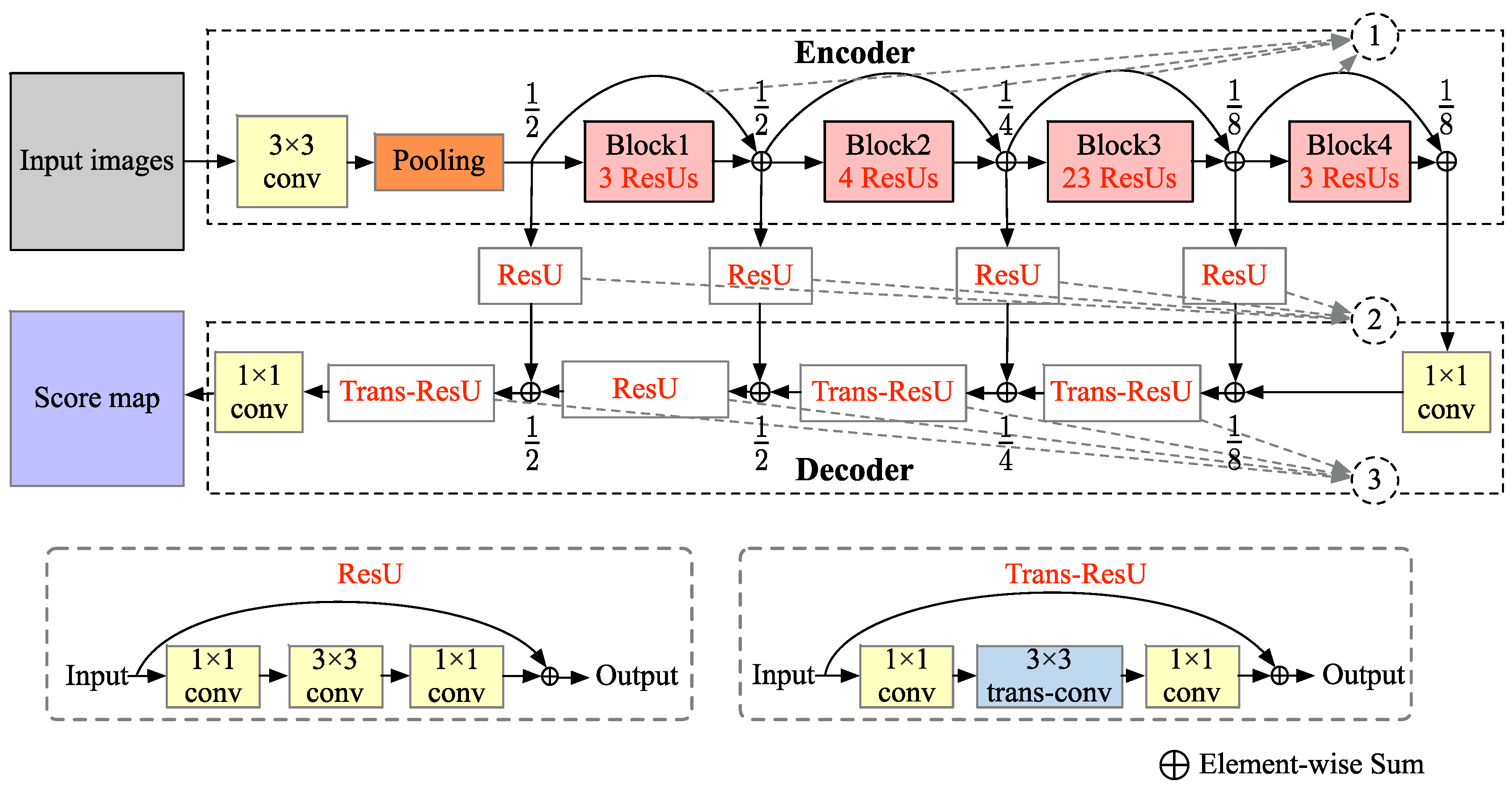
  • A multiconnection ResNet is proposed to fuse multilevel deep features corresponding to different layers of the FCN. The multiconnection residual shortcuts make it possible for low-level features to learn to cooperate with high-level features without introducing redundant information from the low-level features.
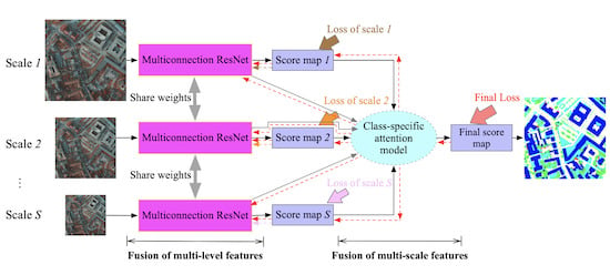
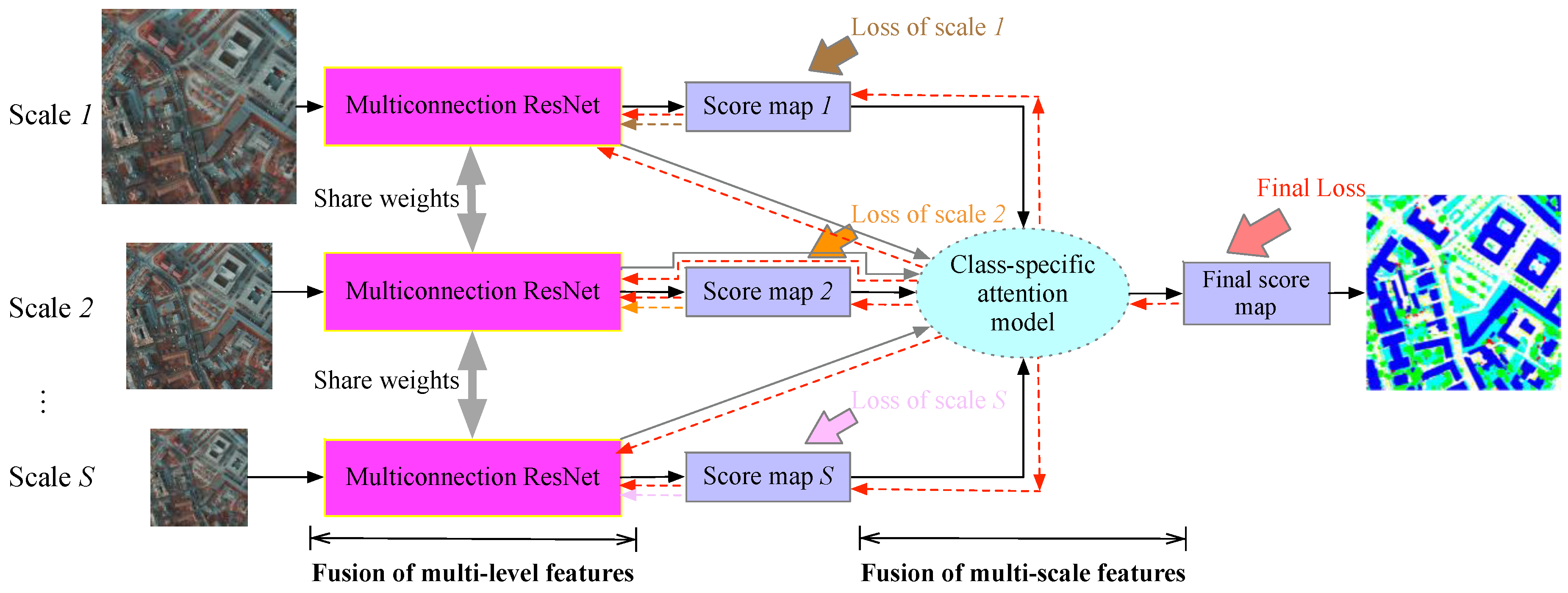
  • A class-specific attention model is proposed to combine multiscale features. It can learn the contributions of various features for each geo-object at each scale. Thus, a class-specific scale-adaptive classification map can be achieved.
  • A novel, end-to-end FCN is developed to integrate the multiconnection ResNet and class-specific attention model into a unified framework.
The remainder of this paper is organized, as follows: Section 2 reviews related works. In Section 3, the framework and main components of the proposed method are presented. Section 4 gives the experimental results and comparisons. A discussion is provided and conclusions are drawn in Section 5 and Section 6, respectively.

2. Related Works

The remote sensing community has invested a great deal of effort into developing advanced effective methods for the classification of VHR images in recent years. A comprehensive review of existing approaches is beyond the scope of this paper. Here, we focus on CNN-related methods of image classification.

2.1. From Convolutional Neural Networks to Fully Convolutional Networks

CNN-based methods are state-of-the-art tools for image analysis tasks and achieve competitive performance in many benchmarks and contests [14]. A standard CNN consists of multiple convolutional layers (often combined with pooling layers) and it is ended by one or more fully connected layers. As shown in Figure 1a, a CNN that is designed for a classification task receives an image as input and produces a probability distribution over different classes as output. The class label with the maximum probability is allocated to the input image as its predicted label. In this regard, a standard CNN is more suitable for solving the problem of image-level labelling.
However, a dense class map is often expected for remote sensing image classification. In other words, a pixel-level labelling result is required. For this reason, great attention is devoted to the development of sophisticated strategies that are based on the CNN for image classification. Patch-based CNN models are widely used approaches, in which the class label for each pixel is predicted by performing patch-level labeling for the neighboring block around the target pixel while using the CNN [27,28,29,30,31]. The patches can be derived by sliding-window [29,30] and segmentation [18,31]. The main reason to use patches for classification is that the standard CNN has at least one fully connected layer and it therefore requires input images with a fixed size. However, this technique ignores the relationship between patches and it yields huge redundant computations [32]. As an alternative, the FCN is proposed to popularize CNN architectures by replacing the fully connected layers with convolutional layers. In this way, dense classification with lower resolution can be achieved, as shown in Figure 1b. The FCN allows for classification maps to be generated for input images of any size and it is also much faster than the patch-based CNN models [33]. Currently, almost all of the state-of-the-art CNN-related methods for pixel-level labelling are developed based on FCN.

2.2. Fusion of Multilevel Deep Features

Multiple stages of pooling and convolutional layers in the FCN progressively down-sample the initial image, which generates low-resolution feature maps that are accompanied by the loss of spatial details and finer structures. This presents challenges for exact alignment of class maps for pixel-level labelling tasks. It is necessary to incorporate low-level features to address this issue, which is beneficial for characterizing boundaries and details, together with high-level features to refine the classification results. One group of approaches for the fusion of multilevel features is referred to as the encoder–decoder paradigm, which includes FCN-8 [20], U-Net [34], DeconvNet [24], and SegNet [21]. In the encoder stage, these methods use multiple stacks of convolutional and pooling layers to obtain hierarchical features at different levels. During the decoder stage, these learned features are then used to up-sample the feature maps with low resolution to higher-resolution classification maps. However, this kind of method directly concatenates or adds the low- and high-level features together as a joint representation, which may introduce redundant information from the low-level features, leading to an adverse impact on the accuracy of the classification results. Two types of methods have been exploited in order to conduct multilevel feature fusion in a better way. The first one designs several gates to select the useful information from the low-level features when fusing features from different levels [26,35]. However, designing proper gates is a nontrivial task, especially without the necessary prior knowledge. The second method attempts to directly add or concatenate multilevel features, followed by a latent fitting strategy, which is expected to eliminate adverse effects brought by the redundant information [25]. Although this method has achieved impressive classification, the postprocessing scheme still has difficulty in removing the redundancy between the features at different levels.
There is another type of strategy to embed low-level features that draws support from extra methods or data. For example, conditional random field (CRF) models are used as a postprocessing step to improve the classification by imposing a smoothness prior in low-level vision, so that neighboring pixels are more likely to be allocated the same class label [36]. An object-based classification method, which is adequate for describing boundaries of geo-objects by image segmentation, is combined with abstracted deep features to increase the classification accuracy [31,37]. In addition, a variety of methods are used in an attempt to add additional data to the FCN, such as digital surface models (DSM), vegetation indices (VI), and edge information [38,39,40,41]. Although these strategies can work well to some extent, they rely on extra handcrafted methods, and the additional data are not always available. In this paper, we aim to develop a novel end-to-end FCN to achieve state-of-the-art performance without introducing extra methods or additional data.

2.3. Fusion of Multiscale Deep Features

It is essential to exploit multiscale features in the FCN setting since various objects are always presented in images to be classified in the form of multiple scales. To this end, two major types of FCN architecture have been proposed. The first is to generate multiscale features in the last few layers by cascading. ParseNet uses global average pooling to produce more abstract features and then combines them with the original feature map [42]. The pyramid scene parsing network (PSPNet) then extends ParseNet by applying multiple global average pooling layers to generate hierarchical scale features [43]. Additionally, dilated convolution is applied to generate multiscale features [44]. However, for these methods, the output map needs to be resampled to the resolution of the input image, which may blur the fine objects or parts. The second type first creates a multiscale representation of the original images and then feeds them through the network. For example, a Laplacian pyramid can be employed to pass images from each scale through a shared network and fuse the features across all scales [45]. Some studies directly represent the original input as resized versions of several scales and fuse multiple features across all scales following a coarse-to-fine sequence [46,47]. When compared to the first method, the second method can directly acquire multiscale features by means of a multiscale representation of the original images, but it usually treats features at each scale for fusion equally. In other words, the different contributions of multiscale features for classifying various objects are not considered.
To overcome these shortcomings, an attention mechanism that aims to generate a specific weight for each scale is applied to fuse the multiscale features in the FCN [48]. However, the main problem of this technique is that the weight is shared for all objects in each scale. Yet, it may be more reasonable that various objects are assigned different weights in each scale.

3. Deep Feature Fusion for Classification of VHR Remote Sensing Images

We present our approach for classification of VHR remote sensing images by fusing deep features with integration of residual connections and an attention model to solve the above two problems regarding deep feature fusion, i.e., avoid introducing redundant information and consider the contributions of features when fusing multiscale features. Figure 2 illustrates a schematic diagram of the proposed method. As can be seen, an input image is resampled to different sizes to produce a multiscale representation as the input of a shared deep network. The proposed network is based on two modules, a multiconnection ResNet and a class-specific attention model. In the following, we describe three main aspects of the proposed method: (1) the multiconnection ResNet for fusion of multilevel features, (2) the class-specific attention model for fusion of multiscale features, and (3) the model learning and inference.

3.1. Multiconnection ResNet for Fusion of Multilevel Features

As shown in Figure 3, the detailed architecture of the proposed multiconnection ResNet is an encoder-decoder network. The encoder part is based on the residual network (ResNet), with 101 layers [49]. The ResNet is mainly constructed of four blocks, each of which contains several stacked residual units (ResUs). The fully connected layer and the average pooling layer at the end of the original ResNet are removed in order to get the dense feature map. The resolution of output feature maps is resampled to one-eighth of the original image in the encoder stage by using dilated convolution following a similar strategy as in [36]. During the decoder stage, the designed transposed residual units (Trans-ResUs) are applied to up-sample the low-resolution feature maps to higher-resolution classification maps. Different from ResU, the middle convolution in Trans-ResU is changed to the transposed convolution. ResU fuses the multiple features that are generated by previous layers in the encoder stage during the up-sampling process.
However, there is one potential problem that is associated with a traditional encoder-decoder deep network: it is difficult to effectively fuse multilevel features without incorporating feature redundancies, which can adversely influence the classification accuracy. The proposed multiconnection ResNet is intended to make low-level features learn how to cooperate with high-level features to address this problem, which is achieved by stacked convolutional layers. Nevertheless, as pointed out in [49], it may be difficult for the stacked convolution layers to directly learn how to cooperate with high-level features in deep networks. For this reason, we add one type of residual connection to these layers between the encoder and decoder. These layers and added residual connections constitute the residual units between the encoder and decoder, as shown in Figure 3. To be specific, given a low-level feature map f that is generated by the encoder, let F ( · ) denote a mapping of the stacked convolutional layers and H ( · ) be the desired underlying mapping to make low-level features learn to cooperate. The stacked convolutional layers are expected to fit another mapping, F ( · ) instead of directly learning the mapping H ( · ) , which is called the residual mapping [49]:
F ( · ) : = H ( · ) f .
Thus, the desired H ( · ) can be recast into F ( · ) + f .
On the other hand, the depth of the network is increased by adding stacked convolutional layers in the encoder and decoder parts, which will result in a potential degradation problem, i.e., as the depth of the network increases, the accuracy becomes saturated and then rapidly degrades [49]. Two more types of residual connection are added to the proposed multiconnection ResNet in order to reduce this phenomenon, as shown in Figure 3: residual connections between residual blocks in the encoder part, and residual connections in ResU and Trans-ResU in the decoder part. As described in [25], the third type of residual connections can also act as the correction of the latent fitting residual between multi-level feature if the learning of ResUs between encoder and decoder parts is insufficient.

3.2. Class-Specific Attention Model for Fusion of Multiscale Features

A class-specific attention model is proposed to fuse multiscale features to improve the multiconnection ResNet further, as shown in Figure 4. Different from direct fusion methods, e.g., averaging or concatenating, which ignore the importance of multiple features at different scales, this model aims to learn the different contributions of various features for each geo-object in each scale.
To be specific, each original input image is resized into a set of scales s { 1 , , S } while using bilinear resampling. Each resized image is passed through a shared multiconnection ResNet. First, a ResU and a separate 1 × 1 convolutional layer for each scale are applied to generate the weight score maps in the class-specific attention model. Mathematically, let g c s ( x i ) denote the weight score for class c at scale s corresponding to the i th pixel x i in the weight score map, where c { 1 , , C } stands for the geo-object class. Obviously, S and C represent the number of scales and geo-objects, respectively. Subsequently, a softmax function in the scale space is adopted to obtain the specific class weight α c s ( x i ) for each scale:
α c s ( x i ) = e x p ( g c s ( x i ) ) s = 1 S e x p ( g c s ( x i ) ) .
Finally, the final classification score of the i th pixel, f c ( x i ) , can be computed though a weighted sum of score maps across all scales:
f c ( x i ) = s = 1 S α c s ( x i ) f c s ( x i ) ,
where f c s ( x i ) is the classification score map of scale s , which is generated by a specific 1 × 1 convolutional layer that is applied to the output of the multiconnection ResNet. Classification results can be inferred based on f c ( x i ) .

3.3. Model Learning and Inference

For pixel-level image classification, each pixel x i can be allocated a class label with the maximum posterior probability:
c i * = a r g m a x c C P c ( x i ; θ ) ,
where c i * denotes the most likely class label for pixel x i and P c ( x i ; θ ) stands for the posterior probability of allocating class c , which can be obtained by the proposed FCN model with parameter θ . To be specific, P c ( x i ; θ ) can be calculated by a softmax function across all classes:
P c ( x i ; θ ) = e x p ( f c ( x i ) ) c = 1 C e x p ( f c ( x i ) ) .
Thus, the image classification problem is equivalent to estimating the optimal parameter θ .
A typical FCN often contains millions of parameters, which are learned by minimizing the losses defined by the difference between the prediction and the ground truth. Multiple intermediate losses that are generated by various network branches corresponding to different scales and the final loss are used jointly to train the network in the learning stage for the proposed FCN. Specifically, the total loss L o s s T can be expressed as the sum of the final loss and intermediate losses of different scales, which is given by
L o s s T = L o s s ( P ( x ; θ ) , y ) + 1 S s = 1 S L o s s ( P ( x s ; θ ) , y s ) ,
where x denotes the original input image and y denotes the associated ground truth map, and x s and y s denote the resized image and ground truth map corresponding to scale s , respectively. The L o s s function is defined as
L o s s ( P ( x ; θ ) , y ) = 1 N i = 1 N c = 1 C y i ( c ) l o g P c ( x i ; θ ) ,
where N is the number of pixels in the input image and y i ( c ) represents y i ( c ) = 1 if the value of y i = c, otherwise y i ( c ) = 0.
The stochastic gradient descent (SDG) algorithm is applied to train the proposed network. Thus, the first derivatives of the parameters in the network need to be calculated to update the parameters during the training stage, which is given by
θ θ η L o s s θ ,
where η is the learning rate. We use the chain rule to obtain the derivative of each parameter. The dashed arrow in Figure 2 denotes the flow of loss. For clarity, the details of L o s s / θ are not presented here; the reader is referred to textbooks, such as [50].
At the inference stage, the network is initialized by the learned parameters from the training stage. The image that is to be classified is resized into multiple scales of images, which are fed into the network to get the classification score map for each scale by the shared multiconnection ResNet. The class-specific attention model first calculates the weight for each scale, and then fuses the feature maps to generate the final prediction map.

4. Experiments

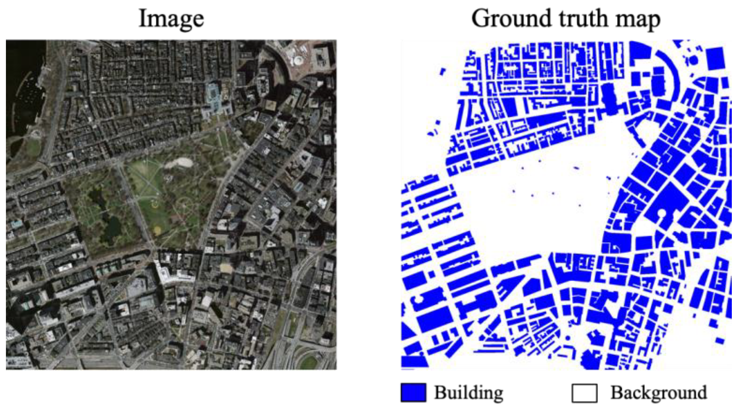
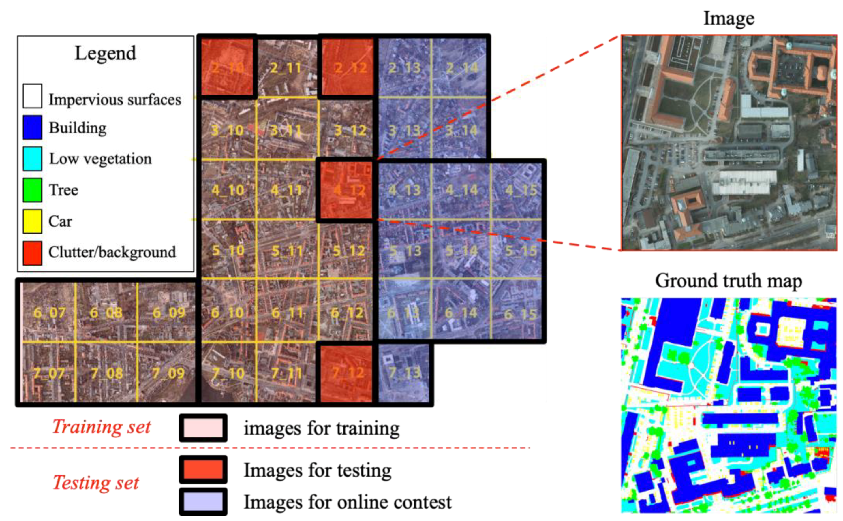
4.1. Experimental Data

Two open datasets of aerial image labelling were selected to evaluate the proposed method—the Massachusetts building dataset and the International Society for Photogrammetry and Remote Sensing (ISPRS) Potsdam dataset.
(1) Massachusetts building dataset. This dataset includes a collection of 151 aerial images that are the Boston area produced by [51]. There are three channels for each image: red (R), green (G), and blue (B). Each image has a size of 1500 × 1500 pixels with about 1 m spatial resolution. The two classes in the ground truth map are buildings and background. The ground truth maps of all these images are available for reference. Figure 5 shows a sample image and its corresponding ground truth map. In this experiment, the dataset was split into a training set of 137 images and a testing set of 14 images.
(2) ISPRS Potsdam dataset. This dataset is provided in the framework of the ISPRS Potsdam 2D Semantic Labeling Contest, which includes 38 images with 6000 × 6000 pixels and about 0.05 m spatial resolution, as shown in Figure 6. There are four channels for each image: near infrared (NIR), R, G, and B; corresponding DSM and nDSM data are also available. Six land cover classes are distributed in the dataset: impervious surfaces, buildings, low vegetation, trees, cars, and clutter/background. The clutter/background class corresponds to a mixture of some geo-objects that are not of interest in our classification experiment. The ground truth maps of 24 images are offered and the organizers for the online contest keep the other 14 images. The organizers ended the online competition in the summer of 2018 and published all of the data. In the experiments, we split the 24 images with available ground truth maps into a training set of 20 images and a testing set of four images, which are shown in Figure 6. We extended the testing set with the other 14 images that are used for online contest to make the division more balanced. It should be noted that only three channels (NIR, R, G) were used for training and testing in the experiments.

4.2. Experimental Setup

4.2.1. Methods for Comparison

Six state-of-the-art methods were compared with the proposed methods for both datasets in the experiments. Descriptions of these models (including our models) are as follows:
  • Multiconnection ResNet: This is the first component of our proposed model, which introduces multiconnection residual shortcuts to make it possible for the convolutional layers to fuse multilevel deep features corresponding to different layers of the FCN. Multiconnection ResNet is referred to as mcResNet for convenience.
  • Integration of multiconnection ResNet and class-specific attention model: This is the proposed end-to-end FCN, which integrates the multiconnection ResNet and class-specific attention model into a unified framework. For convenience, the proposed FCN is referred to as mcResNet-csAM.
  • FCN-8s: There are three variants of FCN models: FCN-32s, FCN-16s, and FCN-8s. We chose FCN-8s for comparison, which has been shown to achieve better classification performance than its counterparts [20].
  • SegNet: SegNet was originally proposed for the semantic segmentation of roads and indoor scenes [21]. The main novelty of SegNet is that the decoder performs the nonlinear up-sampling according to max pooling indices in the encoder. Thus, SegNet can provide good performance with little time and space complexity.
  • Global convolutional network (GCN): GCN is proposed to address both the classification and localization issues for semantic segmentation [52]. It achieves state-of-the-art performance on two public benchmarks: PASCAL VOC 2012 and Cityscapes.
  • RefineNet: RefineNet is proposed to perform semantic segmentation, which is based on ResNet [53]. It achieves state-of-the-art performance on seven public datasets, including PASCAL VOC 2012 and NYUDv2. The RefineNet based on ResNet-101 was compared with ours in the experiments.
  • PSPNet: PSPNet, which introduces the pyramid pooling module to fuse hierarchical scale features, is proposed for scene parsing and semantic segmentation [43]. It ranked first in the ImageNet scene parsing challenge in 2016. We used the modified ResNet-101 as the backbone of PSPNet in the experiments following the official implementation. In the training phase, we also used the auxiliary loss with the weight of 0.4.
  • DeepLab V3+: DeepLab is proposed to conduct semantic segmentation by employing multiple dilated convolutions in the cascade to capture multiscale context, being motived by the fact that atrous/dilated convolutions can easily increase the field of view [54]. When compared with DeepLab V3, the DeepLab V3+ includes a simple decoder part to refine the results [55].

4.2.2. Evaluation Criteria

Two quantitative criteria were used in the experiments to evaluate the classification results of the above methods, F1 score (F1) and overall accuracy (OA). The F1 score can be calculated as
F 1 = 2 × p r e c i s i o n × r e c a l l p r e c i s i o n + r e c a l l ,
where precision and recall can be represented as
p r e c i s i o n = T P T P + F P , r e c a l l = T P T P + F N .
Here, TP, TN, FP, and FN stand for true positive, or the number of correct predictions that an instance is positive; true negative, or the number of correct predictions that an instance is negative; false positive, or the number of incorrect positive predictions; and false negative, or the number of incorrect negative predictions. OA can be obtained by
O A = T P + T N T P + F P + F N + T N ,
Moreover, visual comparison is also utilized to evaluate the results.

4.2.3. Parameter Setting

In the experiments, each image in both datasets was not fed directly to the networks, being limited by GPU memory. Instead, patches had to be cropped from raw images as input to train the networks. In detail, at each training step, patches of 320 × 320 pixels are sampled from a random position of the original images. One or combined operations randomly process these extracted patches to augment the training data: mirror, rotation, and Gaussian blur. In the inference stage, a fixed stride is set to obtain the overlapped patches as inputs. The final predictions on the overlapping regions are averaged, which can reduce the border effects and improve the overall accuracy. In the experiments, the stride was empirically set to 59 pixels for the Massachusetts building dataset and 80 pixels for the ISPRS Potsdam dataset. The models were trained by using stochastic gradient descent (SGD) with momentum. We set the momentum to 0.9 and the weight decay to 0.0005. In addition, inspired by the work in [43], we applied the poly-like learning rate rule, i.e., the learning rate can be represented by base one multiplying ( 1 t / T ) p o w e r . Here, t and T denote the current iteration and maximum iteration, respectively. The base learning rate was set to 0.01 and the power variable was set to 0.9. All of the models were trained with a batch size of five and a total of 1,000,000 iterations. For the proposed model, three scales of input images were fed to the network: 0.5, 0.75, and 1 times the size of the original images (denoted as Scales = {1, 0.75, 0.5}).
For different convolutional network methods, the same parameter settings are configured as much as possible for a fair comparison. However, some hyperparameters that are specific to various models (e.g., momentum and weight decay) may be differently specified in order to make models converge quickly during the training stage. Furthermore, all of the models are trained while using the transfer learning technique. To be specific, the pretrained model based on PASCAL VOC 2012 is transferred to initialize all of the models for comparison in our experiments. It should also be noted that our proposed methods and GCN only use the pretrained parameters of PASCAL VOC 2012 to initialize the encoder part of the models and adopt the normal distribution to initialize other parts, in contrast to other approaches.
Python 3.6 on a Linux platform implements all models in the experiments. The deep learning algorithms are based on TensorFlow. The full implementation (based on TensorFlow) and the trained network are available at GitHub (https://github.com/WindWang2/Multi-connection-attention-networks). The experiments were run on two Intel® Xeon® 8-core CPU @ 2.2 GHz processors with a GPU of Nvidia® GTX1080Ti (11 GB).

4.3. Comparison of Classification Results

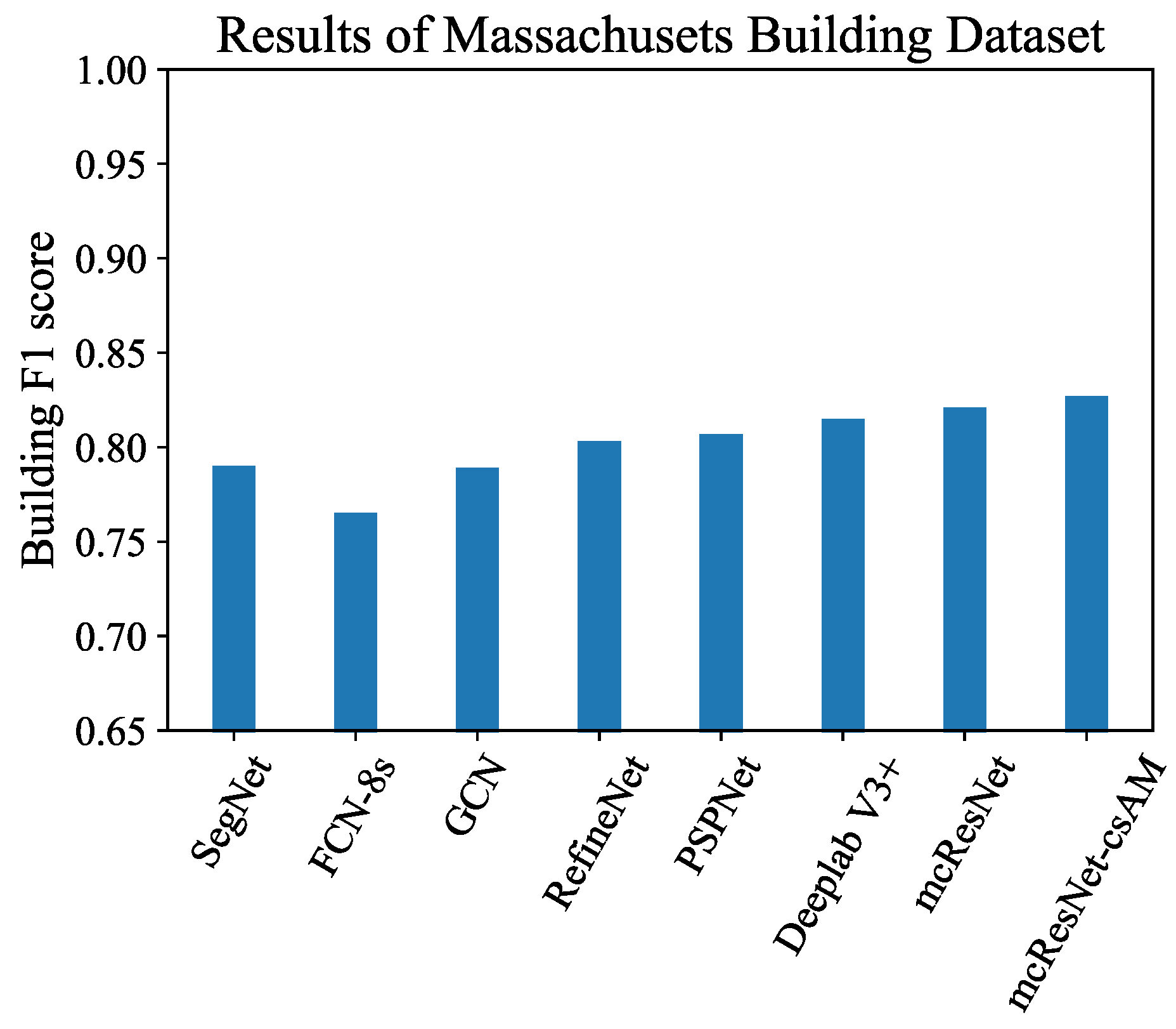
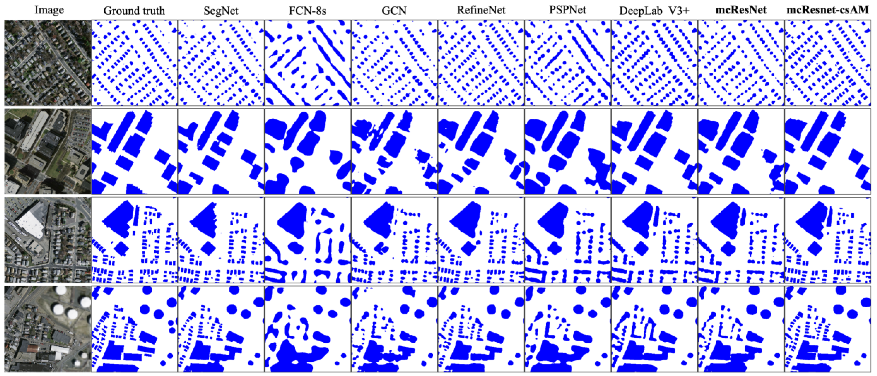
4.3.1. Results of Massachusetts Building Dataset

For the quantitative aspect, Table 1 reports two evaluation criteria of classification results for the different methods, and Figure 7 shows a corresponding bar chart of F1 scores. The proposed mcResNet-csAM yields the highest values of F1 and OA when compared to other methods, achieving the best overall classification performance. In particular, our mcResNet still obtained the second highest F1 despite the lack of the class-specific attention model component, indicating that the multiconnection residual shortcuts are effective for combining high-level abstract features and low-level features for classification. DeepLab V3+ achieved comparable results with the third best F1 and the second better OA.
Four image patches containing buildings with different sizes and shapes were selected for visual comparison, as shown in Figure 8. It can be observed that FCN-8s performed the worst in identifying various sizes of buildings. To be specific, FCN-8s was not able to detect each single instance for small buildings, but could only identify building areas with blurred boundaries. The results of GCN, DeepLab V3+, RefineNet, PSPNet, and mcResNet are significantly better. However, they are still inadequate for preserving the shape details and fine edges. In addition, the classification results of large buildings by GCN are not homogeneous enough. SegNet can perform better in detecting small buildings, but it results in more false negatives, especially for large buildings. In contrast, mcResNet-csAM can achieve scale-adaptive classification results by taking the multiscale nature of various geo-objects into account, i.e., large buildings appear more homogeneous, and small buildings are detected with well-preserved structural details and boundaries. This confirms that our proposed end-to-end FCN is able to fuse the multilevel and multiscale deep features to enhance classification performance.

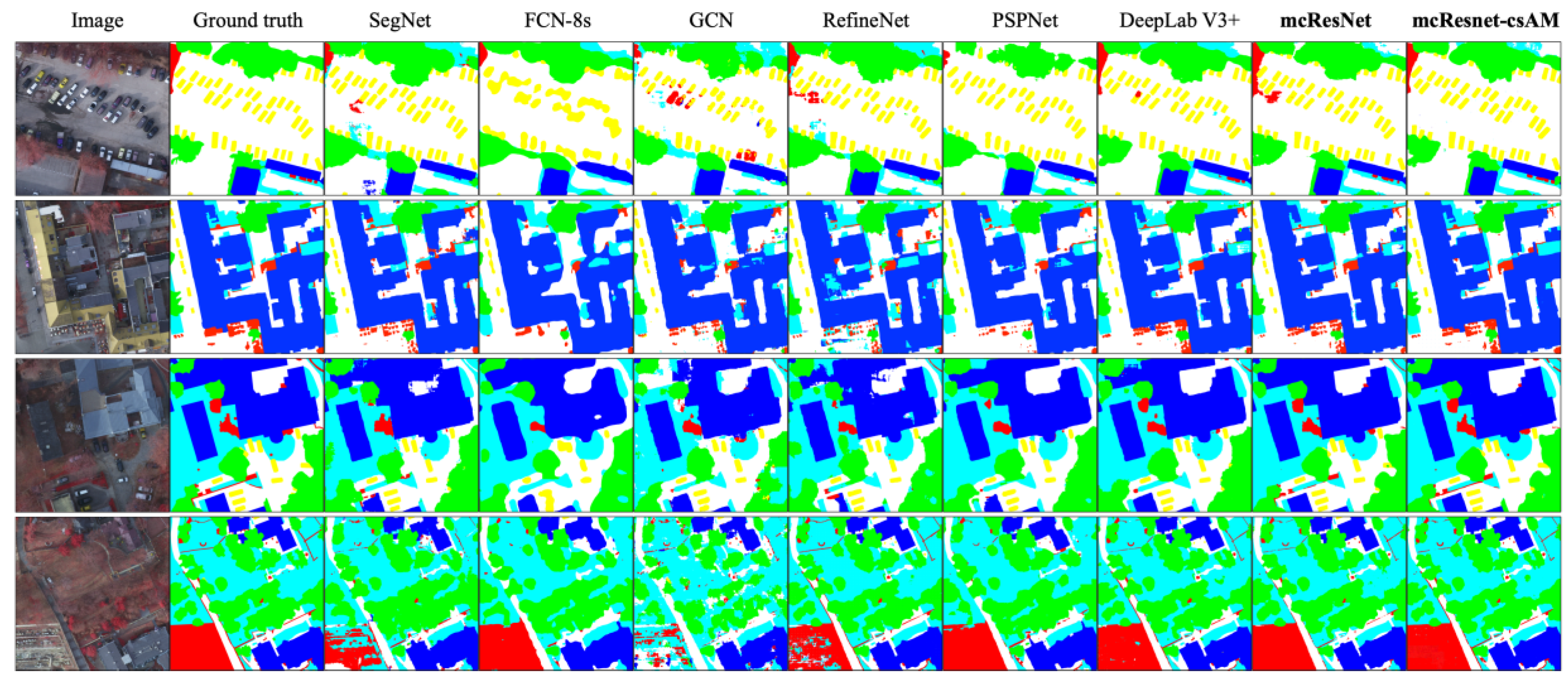
4.3.2. Results of ISPRS Potsdam Dataset

Table 2 and Figure 9 report the F1 scores and OA for different methods. It can be observed that (1) mcResNet-csAM outperforms other methods overall, although DeepLab V3+ can achieve optimal F1 scores for low vegetation with slight improvements and (2) mcResNet shows comparative performance with other methods, except mcResNet-csAM. This reveals the advantages of the proposed approach. Specifically, the proposed mcResNet-csAM and mcResNet exhibit obviously greater F1 values than other methods for classifying cars.
Four image patches with different scenes were selected for visual comparison, as illustrated in Figure 10. Similar to the experiment for the Massachusetts building dataset, for FCN-8s, large-scale buildings are well classified, while small-scale cars are detected with blurred boundaries. Classification by GCN is improved with regard to preserving detailed information, but the classification maps seem to be not as compact as those of other methods, resulting in the degradation of classification accuracy. The results of SegNet and RefineNet are better than GCN and FCN-8s, but both of them obtained some commission errors, especially for the class of buildings. Moreover, more coherent labelling with precise edges and preserved boundaries can be achieved by the proposed methods although the results of PSPNet, and DeepLab V3+ are very close to those of the proposed methods. In addition, benefiting from the ability to learn the contributions of various features for each geo-object in each scale, mcResNet-csAM compares favorably with mcResNet, in the respect of the scale-adaptive classification of various geo-objects.

4.4. Results of ISPRS Potsdam 2D Semantic Labeling Contest

The ISPRS Work Group III/4 held an online contest of two-dimensional (2D) semantic labeling for the Potsdam dataset. The participants sent the classified results of 14 images for which ground truth maps were not provided to the organizers for evaluation. All of the participants’ results are published on the website (http://www2.isprs.org/commissions/comm2/wg4/potsdam-2d-semantic-labeling.html), which now includes more than 50 methods. We submitted the results of our proposed mcResNet-csAM (ID: SWJ_2) to compare with the competitors’ methods. All of the settings were the same as those of the above experiments, with one difference: we retrained mcResNet-csAM by using all 24 images. The 10 methods (including our method) with the highest overall accuracy were selected for comparison (Table 3). Statistics in Table 3 show that the proposed method ranks #1 in terms of overall accuracy, with the highest value of 91.7%, although images with only three channels (NIR, R, G) were used to train the network, and neither the additional DSM data nor any postprocessing strategies were applied. Moreover, mcResNet-csAM achieved the optimal F1 score for impervious surfaces. When compared with the methods that did not use DSM, the best F1 scores for low vegetation and buildings could be also obtained by mcResNet-csAM. Therefore, the results clearly demonstrate the positive impact of a synergistic use of multilevel and multiscale deep features in the proposed FCN unified framework, pointing out the advantages of the proposed approach.

5. Discussion

5.1. Effect of Scale Setting

For the proposed mcResNet-csAM, various scales of input images, which form a multiscale representation, are fed to the network for training. It is necessary to discuss the effect of scale setting because the settings of scale parameters may affect the performance of our methods. It should be noted that the four images (denoted as the red in the Figure 6) with corresponding ground truth maps were used to evaluate the proposed mcResNet-csAM with different scale settings.
Specifically, five settings on the composition of scales were analyzed for both datasets: Scales = {1, 0.75}, {1, 0.5}, {1, 0.75, 0.5}, {1, 0.5, 0.25}, and {1, 0.75, 0.5, 0.25}. It should be noted that mcResNet-csAM is equivalent to mcResNet for scale setting {1}. Table 4 shows the values of mean F1 and OA against the different scale settings for both two datasets. We would like to stress that, for the building extraction task in the Massachusetts building dataset, only F1 values are used for analysis. As can be observed, mcResNet-csAM with Scales = {1, 0.75, 0.50} achieved the best performance for both datasets. For the Massachusetts building dataset, the mean F1 values do not vary much when various Scales are set, i.e., {1, 0.75, 0.5}, {1, 0.75}, and {1, 0.5}. Adding {0.5} and {0.75} to Scales slightly increases the accuracy, whereas adding {0.25} to Scales will result in a drop in performance. The reason may be that incorporating the scales of {0.5} and {0.75} can be helpful to impose attention to scale on middle-scale geo-objects, thus enhancing the classification. However, the scale of {0.25} corresponds to a too-coarse resized input image, which introduces more uncertainty. A similar phenomenon can be observed for the ISPRS Potsdam challenge dataset. For this reason, the Scales for the two datasets in our experiments were set to {1, 0.75, 0.5}.

5.2. Comparison of Different Methods for Fusing Multi-Scale Features

We performed comparisons against some other fusion methods, i.e., max pooling, average pooling, and feature pyramid networks (FPN) to show the effectiveness of the proposed attention model for fusing multi-scale features. Max pooling and average pooling are the mostly commonly used methods for fusing features in the neural networks. FPN is proposed by [61], which applies a hierarchical structure to fuse features. In the experiments, we set the Scales to {1, 0.75, 0.5}. We also used the four testing images to validate different fusion methods for the ISPRS Potsdam dataset.
Table 5 lists the results of different methods for fusing multi-scale features. As can be seen, the proposed attention model achieved best score of F1 and OA in both two datasets. FPN and Max pooling get comparable results that are slightly worse than ours. Mean pooling obtains the worst performance, since it may blur some fine part. The results show that the proposed attention model can effectively fuse multi-scale features.

5.3. Complexity Analysis

Table 6 reports the complexity of our method and other state-of-the-art methods. The average of the time to inference 100 patches (320 × 320 pixels) with a GTX 1080Ti GPU measures the time complexity. As shown in Table 6, mcResNet-csAM produces comparable space complexity, while it takes about 12 s more than the most efficient model, SegNet. The extra time is worthwhile, because the network is modeled by processing input images of multiple scales to achieve class-specific, scale-adaptive classification results.

5.4. Effect of Data Quality

In our experiments, some inaccurate ground truth maps were noticed in the above two datasets, such as those that are shown in Figure 11 and Figure 12. For the Massachusetts building dataset, the associated ground truth building labels were retrieved from OpenStreetMap. Some buildings in the images of the dataset are not labeled in the corresponding ground truth maps, and vice versa, due to the time difference between image acquisition and building information collection by OpenStreetMap, as shown in Figure 11. Moreover, annotation errors are also unavoidable, especially for VHR images. For instance, obvious mislabeling also appeared in the ISPRS Potsdam dataset, as illustrated in Figure 12.
One of the interesting things that we observed is that our proposed mcResNet-csAM model can obtain the correct image extraction results, even with inaccurate ground truth maps. Thus, the robustness of the proposed method against label noise has been verified to some extent. On the other hand, it is still necessary to further investigate the effect of improperly labeled samples, owing to human mistakes or limited labeling conditions, which will be carried out in our future work.

6. Conclusions

In this work, a novel FCN that is intended to conduct fusion of deep features was presented to address the problems of VHR image classification. The proposed approach showed impressive performance by focusing on two aspects: (1) A multiconnection ResNet is proposed to fuse multilevel deep features that correspond to different layers of FCNs. The multiconnection residual connections make it possible for low-level features to learn how to cooperate with high-level features. Thus, hierarchical features, i.e., high-level abstract knowledge invariant to pixel-level variations that are useful for locating geo-objects roughly and low-level features that contribute to recovering geo-object boundaries, can be effectively fused without introducing redundant information from the low-level features. (2) A class-specific attention model is proposed to combine multiscale features in the scale space. It can learn the contributions of various features for each geo-object in each scale. In detail, the model generates a class-specific weight map that can softly weight the multiscale features for each pixel site for each geo-object in each scale, and the weighted sum of score maps is then utilized for further classification. In this regard, a class-specific, scale-adaptive classification map can be achieved in the proposed framework.
Extensive experiments indicated that the proposed method outperforms other state-of-the-art methods in two benchmarks and they can achieve scale-adaptive classification results. For the ISPRS online contest, the proposed method achieved the highest OA without using additional DSM data and postprocessing.
Moreover, we presented the studies of the proposed attention model. The results showed that the proposed attention model achieved better performance than other fusion methods.
In future work, we will test the performance of methods when the input data is less perfect. We will also try to make the algorithm more efficient and apply it to other fine-grained classification tasks.

Author Contributions

Conceptualization, Z.L., L.S. and J.W.; methodology, L.S. and J.W.; software, J.W., W.Q. and Y.D.; validation, L.S., J.W. and W.Q.; formal analysis, J.W. and L.S.; writing—original draft preparation, J.W.; writing—review and editing, Z.L. and L.S.; visualization, W.Q. and Y.D.; funding acquisition, Z.L. and L.S.

Funding

This research was funded by the National Key Research and Development Program of China (2016YFB0501403), the National Natural Science Foundation of China (41401374, 41771451), the Environment and Conservation Fund of Hong Kong (K-ZB86) and the MiaoZi project of Sichuan Province in China (2019013).

Acknowledgments

The authors greatly acknowledge the providers of the open source datasets. The Massachusetts Building Dataset is produced by Volodymyr Mnih and the ISPRS Potsdam Challenge Dataset is produced by the International Society for Photogrammetry and Remote Sensing (http://www2.isprs.org/commissions/comm3/wg4/semantic-labeling.html). The authors also thank the anonymous reviewers for providing comments to improve the manuscript.

Conflicts of Interest

The authors declare no conflict of interest.

References

  1. Hunt, E.R.; Daughtry, C.S.T. What good are unmanned aircraft systems for agricultural remote sensing and precision agriculture? Int. J. Remote Sens. 2017, 39, 5345–5376. [Google Scholar] [CrossRef] [Green Version]
  2. Dash, J.P.; Watt, M.S.; Pearse, G.D.; Heaphy, M.; Dungey, H.S. Assessing very high resolution UAV imagery for monitoring forest health during a simulated disease outbreak. ISPRS J. Photogramm. Remote Sens. 2017, 131, 1–14. [Google Scholar] [CrossRef]
  3. Du, P.; Liu, P.; Xia, J.; Feng, L.; Liu, S.; Tan, K.; Cheng, L. Remote Sensing Image Interpretation for Urban Environment Analysis: Methods, System and Examples. Remote Sens. 2014, 6, 9458–9474. [Google Scholar] [CrossRef] [Green Version]
  4. Sevilla-Lara, L.; Sun, D.; Jampani, V.; Black, M.J. Optical flow with semantic segmentation and localized layers. In Proceedings of the IEEE Conference on Computer Vision and Pattern Recognition, Las Vegas, NV, USA, 26 June–1 July 2016; pp. 3889–3898. [Google Scholar]
  5. Gao, P.; Wang, J.; Zhang, H.; Li, Z. Boltzmann Entropy-Based Unsupervised Band Selection for Hyperspectral Image Classification. IEEE Geosci. Remote Sens. Lett. 2019, 16, 462–466. [Google Scholar] [CrossRef]
  6. Shen, L.; Wu, L.; Dai, Y.; Qiao, W.; Wang, Y. Topic modelling for object-based unsupervised classification of VHR panchromatic satellite images based on multiscale image segmentation. Remote Sens. 2017, 9, 840. [Google Scholar] [CrossRef]
  7. Pham, M.T.; Mercier, G.; Michel, J. PW-COG: An effective texture descriptor for VHR satellite imagery using a pointwise approach on covariance matrix of oriented gradients. IEEE Trans. Geosci. Remote Sens. 2016, 54, 3345–3359. [Google Scholar] [CrossRef]
  8. Zhang, X.; Du, S.; Wang, Q.; Zhou, W. Multiscale Geoscene Segmentation for Extracting Urban Functional Zones from VHR Satellite Images. Remote Sens. 2018, 10, 281. [Google Scholar] [CrossRef]
  9. Pham, M.-T.; Mercier, G.; Michel, J. Pointwise graph-based local texture characterization for very high resolution multispectral image classification. IEEE J. Sel. Top. Appl. Earth Obs. Remote Sens. 2015, 8, 1962–1973. [Google Scholar] [CrossRef]
  10. Blaschke, T. Object based image analysis for remote sensing. ISPRS J. Photogramm. Remote Sens. 2010, 65, 2–16. [Google Scholar] [CrossRef] [Green Version]
  11. Shen, L.; Tang, H.; Chen, Y.H.; Gong, A.; Li, J.; Yi, W.B. A semisupervised latent dirichlet allocation model for object-based classification of VHR panchromatic satellite images. IEEE Geosci. Remote Sens. Lett. 2014, 11, 863–867. [Google Scholar] [CrossRef]
  12. Marcos, D.; Volpi, M.; Kellenberger, B.; Tuia, D. Land cover mapping at very high resolution with rotation equivariant CNNs: Towards small yet accurate models. ISPRS J. Photogramm. Remote Sens. 2018, 145, 96–107. [Google Scholar] [CrossRef] [Green Version]
  13. Hinton, G.E.; Osindero, S.; Teh, Y.W. A fast learning algorithm for deep belief nets. Neural Comput. 2006, 18, 1527–1554. [Google Scholar] [CrossRef] [PubMed]
  14. Krizhevsky, A.; Sutskever, I.; Hinton, G.E. Imagenet classification with deep convolutional neural networks. In Proceedings of the Advances in Neural Information Processing Systems, Lake Tahoe, NV, USA, 3–8 December 2012; pp. 1097–1105. [Google Scholar]
  15. Ye, D.; Li, Y.; Tao, C.; Xie, X.; Wang, X. Multiple Feature Hashing Learning for Large-Scale Remote Sensing Image Retrieval. ISPRS Int. J. Geo-Inf. 2017, 6, 364. [Google Scholar] [CrossRef]
  16. Li, E.; Xia, J.; Du, P.; Lin, C.; Samat, A. Integrating Multilayer Features of Convolutional Neural Networks for Remote Sensing Scene Classification. IEEE Trans. Geosci. Remote Sens. 2017, 55, 5653–5665. [Google Scholar] [CrossRef]
  17. Zheng, X.; Yuan, Y.; Lu, X. A Deep Scene Representation for Aerial Scene Classification. IEEE Trans. Geosci. Remote Sens. 2019, 57, 4799–4809. [Google Scholar] [CrossRef]
  18. Zhang, C.; Sargent, I.; Pan, X.; Li, H.; Gardiner, A.; Hare, J.; Atkinson, P.M. An object-based convolutional neural network (OCNN) for urban land use classification. Remote Sens. Environ. 2018, 216, 57–70. [Google Scholar] [CrossRef] [Green Version]
  19. LeCun, Y.; Boser, B.E.; Denker, J.S.; Henderson, D.; Howard, R.E.; Hubbard, W.E.; Jackel, L.D. Handwritten digit recognition with a back-propagation network. In Proceedings of the Advances in Neural Information Processing Systems, Denver, CO, USA, 26–29 November 1990; pp. 396–404. [Google Scholar]
  20. Long, J.; Shelhamer, E.; Darrell, T. Fully convolutional networks for semantic segmentation. In Proceedings of the IEEE Conference on Computer Vision and Pattern Recognition, Boston, MA, USA, 8–12 June 2015; pp. 3431–3440. [Google Scholar]
  21. Badrinarayanan, V.; Kendall, A.; Cipolla, R. SegNet: A deep convolutional encoder-decoder architecture for image segmentation. IEEE Trans. Pattern Anal. Mach. Intell. 2017, 39, 2481–2495. [Google Scholar] [CrossRef]
  22. Li, Y.; Chen, Y.; Liu, G.; Jiao, L. A Novel Deep Fully Convolutional Network for PolSAR Image Classification. Remote Sens. 2018, 10, 1984. [Google Scholar] [CrossRef]
  23. Fu, G.; Liu, C.; Zhou, R.; Sun, T.; Zhang, Q. Classification for high resolution remote sensing imagery using a fully convolutional network. Remote Sens. 2017, 9, 498. [Google Scholar] [CrossRef]
  24. Noh, H.; Hong, S.; Han, B. Learning deconvolution network for semantic segmentation. In Proceedings of the IEEE International Conference on Computer Vision, Santiago, Chile, 13–16 December 2015; pp. 1520–1528. [Google Scholar]
  25. Liu, Y.; Fan, B.; Wang, L.; Bai, J.; Xiang, S.; Pan, C. Semantic labeling in very high resolution images via a self-cascaded convolutional neural network. ISPRS J. Photogramm. Remote Sens. 2018, 145, 78–95. [Google Scholar] [CrossRef] [Green Version]
  26. Wang, H.; Wang, Y.; Zhang, Q.; Xiang, S.; Pan, C. Gated convolutional neural network for semantic segmentation in high-resolution images. Remote Sens. 2017, 9, 446. [Google Scholar] [CrossRef]
  27. Pan, B.; Shi, Z.; Zhang, N.; Xie, S. Hyperspectral image classification based on nonlinear spectral–spatial network. IEEE Geosci. Remote Sens. Lett. 2016, 13, 1782–1786. [Google Scholar] [CrossRef]
  28. Gaetano, R.; Ienco, D.; Ose, K.; Cresson, R. A Two-Branch CNN Architecture for Land Cover Classification of PAN and MS Imagery. Remote Sens. 2018, 10, 1746. [Google Scholar] [CrossRef]
  29. Perez, D.; Banerjee, D.; Kwan, C.; Dao, M.; Shen, Y.; Koperski, K.; Marchisio, G.; Li, J. Deep learning for effective detection of excavated soil related to illegal tunnel activities. In Proceedings of the IEEE Ubiquitous Computing, Electronics and Mobile Communication Conference, New York, NY, USA, 19–21 October 2017; pp. 626–632. [Google Scholar]
  30. Lu, Y.; Perez, D.; Dao, M.; Kwan, C.; Li, J. Deep Learning with Synthetic Hyperspectral Images for Improved Soil Detection in Multispectral Imagery. In Proceedings of the IEEE Ubiquitous Computing, Electronics and Mobile Communication Conference, New York, NY, USA, 8–10 November 2018; pp. 8–10. [Google Scholar]
  31. Zhao, W.; Du, S.; Emery, W.J. Object-based convolutional neural network for high-resolution imagery classification. IEEE J. Sel. Top. Appl. Earth Obs. Remote Sens. 2017, 10, 3386–3396. [Google Scholar] [CrossRef]
  32. Maggiori, E.; Tarabalka, Y.; Charpiat, G.; Alliez, P. Convolutional neural networks for large-scale remote-sensing image classification. IEEE Trans. Geosci. Remote Sens. 2016, 55, 645–657. [Google Scholar] [CrossRef]
  33. Zhong, Z.; Li, J.; Cui, W.; Jiang, H. Fully convolutional networks for building and road extraction: Preliminary results. In Proceedings of the IEEE International Geoscience and Remote Sensing Symposium, Beijing, China, 10–15 July 2016; pp. 1591–1594. [Google Scholar]
  34. Ronneberger, O.; Fischer, P.; Brox, T. U-net: Convolutional networks for biomedical image segmentation. In Proceedings of the International Conference on Medical Image Computing and Computer-Assisted Intervention, Munich, Germany, 5–9 October 2015; pp. 234–241. [Google Scholar]
  35. Yang, H.; Wu, P.; Yao, X.; Wu, Y.; Wang, B.; Xu, Y. Building extraction in very high resolution imagery by dense-attention networks. Remote Sens. 2018, 10, 1768. [Google Scholar] [CrossRef]
  36. Chen, L.-C.; Papandreou, G.; Kokkinos, I.; Murphy, K.; Yuille, A.L. Deeplab: Semantic image segmentation with deep convolutional nets, atrous convolution, and fully connected crfs. IEEE Trans. Pattern Anal. Mach. Intell. 2018, 40, 834–848. [Google Scholar] [CrossRef]
  37. Mboga, N.; Georganos, S.; Grippa, T.; Lennert, M.; Vanhuysse, S.; Wolff, E. Fully Convolutional Networks and Geographic Object-Based Image Analysis for the Classification of VHR Imagery. Remote Sens. 2019, 11, 597. [Google Scholar] [CrossRef]
  38. Audebert, N.; Le Saux, B.; Lefèvre, S. Beyond RGB: Very high resolution urban remote sensing with multimodal deep networks. ISPRS J. Photogramm. Remote Sens. 2018, 140, 20–32. [Google Scholar] [CrossRef] [Green Version]
  39. Cao, R.; Chen, Y.; Shen, M.; Chen, J.; Zhou, J.; Wang, C.; Yang, W. A simple method to improve the quality of NDVI time-series data by integrating spatiotemporal information with the Savitzky-Golay filter. Remote Sens. Environ. 2018, 217, 244–257. [Google Scholar] [CrossRef]
  40. Marmanis, D.; Schindler, K.; Wegner, J.D.; Galliani, S.; Datcu, M.; Stilla, U. Classification with an edge: Improving semantic image segmentation with boundary detection. ISPRS J. Photogramm. Remote Sens. 2018, 135, 158–172. [Google Scholar] [CrossRef] [Green Version]
  41. Zhang, W.; Huang, H.; Schmitz, M.; Sun, X.; Wang, H.; Mayer, H. Effective fusion of multi-modal remote sensing data in a fully convolutional network for semantic labeling. Remote Sens. 2017, 10, 52. [Google Scholar] [CrossRef]
  42. Liu, W.; Rabinovich, A.; Berg, A.C. Parsenet: Looking wider to see better. arXiv 2015, arXiv:1506.04579. [Google Scholar]
  43. Zhao, H.; Shi, J.; Qi, X.; Wang, X.; Jia, J. Pyramid scene parsing network. In Proceedings of the IEEE Conference on Computer Vision and Pattern Recognition, Honolulu, HI, USA, 21–26 July 2017; pp. 2881–2890. [Google Scholar]
  44. Yu, F.; Koltun, V. Multi-scale context aggregation by dilated convolutions. arXiv 2015, arXiv:1511.07122. [Google Scholar]
  45. Farabet, C.; Couprie, C.; Najman, L.; LeCun, Y. Learning hierarchical features for scene labeling. IEEE Trans. Pattern Anal. Mach. Intell. 2013, 35, 1915–1929. [Google Scholar] [CrossRef] [PubMed]
  46. Eigen, D.; Fergus, R. Predicting depth, surface normals and semantic labels with a common multi-scale convolutional architecture. In Proceedings of the IEEE International Conference on Computer Vision, Santiago, Chile, 13–16 December 2015; pp. 2650–2658. [Google Scholar]
  47. Lin, G.; Shen, C.; Van Den Hengel, A.; Reid, I. Efficient piecewise training of deep structured models for semantic segmentation. In Proceedings of the IEEE Conference on Computer Vision and Pattern Recognition, Las Vegas, NV, USA, 26 June–1 July 2016; pp. 3194–3203. [Google Scholar]
  48. Chen, L.-C.; Yang, Y.; Wang, J.; Xu, W.; Yuille, A.L. Attention to scale: Scale-aware semantic image segmentation. In Proceedings of the IEEE Conference on Computer Vision and Pattern Recognition, Las Vegas, NV, USA, 26 June–1 July 2016; pp. 3640–3649. [Google Scholar]
  49. He, K.; Zhang, X.; Ren, S.; Sun, J. Deep residual learning for image recognition. In Proceedings of the IEEE Conference on Computer Vision and Pattern Recognition, Las Vegas, NV, USA, 26 June–1 July 2016; pp. 770–778. [Google Scholar]
  50. Goodfellow, I.; Bengio, Y.; Courville, A. Deep Learning; MIT press: Cambridge, MA, USA, 2016. [Google Scholar]
  51. Mnih, V. Machine Learning for Aerial Image Labeling; University of Toronto (Canada): Toronto, ON, USA, 2013. [Google Scholar]
  52. Peng, C.; Zhang, X.; Yu, G.; Luo, G.; Sun, J. Large Kernel Matters—Improve Semantic Segmentation by Global Convolutional Network. In Proceedings of the IEEE Conference on Computer Vision and Pattern Recognition, Honolulu, HI, USA, 21–26 July 2017; pp. 4353–4361. [Google Scholar]
  53. Lin, G.; Milan, A.; Shen, C.; Reid, I. Refinenet: Multi-path refinement networks for high-resolution semantic segmentation. In Proceedings of the IEEE Conference on Computer Vision and Pattern Recognition, Honolulu, HI, USA, 21–26 July 2017; pp. 1925–1934. [Google Scholar]
  54. Chen, L.-C.; Papandreou, G.; Schroff, F.; Adam, H. Rethinking atrous convolution for semantic image segmentation. arXiv 2017, arXiv:1706.05587. [Google Scholar]
  55. Chen, L.-C.; Zhu, Y.; Papandreou, G.; Schroff, F.; Adam, H. Encoder-decoder with atrous separable convolution for semantic image segmentation. In Proceedings of the European Conference on Computer Vision, Munich, Germany, 8–14 September 2018; pp. 801–818. [Google Scholar]
  56. Sherrah, J. Fully convolutional networks for dense semantic labelling of high-resolution aerial imagery. arXiv 2016, arXiv:1606.02585. [Google Scholar]
  57. Chen, G.; Zhang, X.; Wang, Q.; Dai, F.; Gong, Y.; Zhu, K. Symmetrical dense-shortcut deep fully convolutional networks for semantic segmentation of very-high-resolution remote sensing images. IEEE J. Sel. Top. Appl. Earth Obs. Remote Sens. 2018, 11, 1633–1644. [Google Scholar] [CrossRef]
  58. Yang, H.; Yu, B.; Luo, J.; Chen, F. Semantic segmentation of high spatial resolution images with deep neural networks. GISci. Remote Sens. 2019, 56, 749–768. [Google Scholar] [CrossRef]
  59. Piramanayagam, S.; Schwartzkopf, W.; Koehler, F.W.; Saber, E. Classification of remote sensed images using random forests and deep learning framework. In Proceedings of the SPIE Remote Sensing, Scotland, UK, 26–29 September 2016; p. 100040L. [Google Scholar]
  60. Liu, Y.; Piramanayagam, S.; Monteiro, S.T.; Saber, E. Semantic segmentation of multisensor remote sensing imagery with deep ConvNets and higher-order conditional random fields. J. Appl. Remote Sens. 2019, 13, 016501. [Google Scholar] [CrossRef] [Green Version]
  61. Lin, T.-Y.; Dollár, P.; Girshick, R.; He, K.; Hariharan, B.; Belongie, S. Feature pyramid networks for object detection. In Proceedings of the IEEE Conference on Computer Vision and Pattern Recognition, Honolulu, HI, USA, 21–26 July 2017; pp. 2117–2125. [Google Scholar]
Figure 1. Network architectures of (a) convolutional neural network (CNN) and (b) fully convolutional network (FCN) for classification tasks.
Remotesensing 11 01617 g001
Figure 2. Schematic diagram of proposed method. Dashed arrows indicate the flow of loss in the training stage.
Remotesensing 11 01617 g002
Figure 3. Framework of proposed multiconnection residual network containing several residual units (ResNet). Three types of residual connections are added to ResNet, illustrated by dashed arrows: 1. residual connections between residual blocks in the encoder part; 2. residual connections in ResU between the encoder and decoder; 3. residual connections in ResU and residual network containing transposed residual units (Trans-ResU) in the decoder part. ResU, residual unit; Trans-ResU, transposed residual unit.
Remotesensing 11 01617 g003
Figure 4. Framework of proposed class-specific attention model. Note that only two scales of the original input image are used to illustrate the model, for convenience.
Remotesensing 11 01617 g004
Figure 5. Sample image and corresponding ground truth map in Massachusetts building dataset.
Remotesensing 11 01617 g005
Figure 6. Review of International Society for Photogrammetry and Remote Sensing (ISPRS) Potsdam dataset.
Remotesensing 11 01617 g006
Figure 7. Bar chart of F1 scores of various methods for Massachusetts building dataset.
Remotesensing 11 01617 g007
Figure 8. Qualitative comparison of various methods for Massachusetts building dataset. The first and second columns are image samples to be classified and corresponding ground truth maps, respectively. The other five columns are classification results of various methods; the last two columns are the results of our proposed methods.
Remotesensing 11 01617 g008
Figure 9. Bar chart of F1 scores and OA of various methods for ISPRS Potsdam dataset.
Remotesensing 11 01617 g009
Figure 10. Qualitative comparison of various methods for ISPRS Potsdam dataset. The first and second columns are the image samples to be classified and corresponding ground truth maps, respectively. The other five columns are classification results of various methods; the last two columns are the results of our proposed methods.
Remotesensing 11 01617 g010
Figure 11. (a) Image samples, (b) corresponding ground truth maps, and (c) extraction results by the proposed method mcResNet-csAM in the Massachusetts building dataset.
Remotesensing 11 01617 g011
Figure 12. (a) Image samples, (b) corresponding ground truth maps, and (c) extraction results by the proposed method mcResNet-csAM in the ISPRS Potsdam dataset.
Remotesensing 11 01617 g012
Table 1. F1 (%) and overall accuracy (OA) (%) of various methods for Massachusetts building dataset. GCN, global convolutional network; PSPNet, pyramid scene parsing network; mcResNet, multiconnection ResNet; mcResNet-csAM, multiconnection ResNet/class-specific attention model.
MethodsF1OA
SegNet79.992.9
FCN-8s76.492.9
GCN78.992.8
RefineNet80.393.1
PSPNet80.793.2
DeepLab V3+81.594.2
mcResNet81.694.0
mcResNet-csAM (3 scales)82.794.6
Table 2. F1 (%) and OA (%) of various methods for ISPRS Potsdam dataset.
MethodsImp surf (F1)Building (F1)Low veg (F1)Tree (F1)Car (F1)Mean F1OA
SegNet89.093.787.384.989.288.887.9
FCN-8s87.894.985.683.781.586.787.0
GCN79.694.178.479.385.983.583.3
RefineNet88.194.383.784.988.988.087.2
PSPNet89.895.885.986.088.189.188.8
DeepLab V3+90.996.086.385.789.889.789.5
mcResNet91.695.786.085.890.289.889.5
mcResNet-csAM (3 scales)92.496.286.286.090.390.290.0
Table 3. F1 (%) and OA (%) of various methods for ISPRS Potsdam two-dimensional (2D) semantic labeling contest.
MethodsImp surf (F1)Building (F1)Low veg (F1)Tree (F1)Car (F1)OARemark
AZ3 93.196.387.288.696.090.7with DSM
CASIA2 [25]93.397.087.788.496.291.1
DST_6 [56]92.496.486.887.793.490.2
CVEO [57]91.294.586.487.495.489.0
CAS_Y2 [58]92.696.287.387.795.790.4
RIT6 [59]92.597.086.587.294.990.2
RIT_L7 [60]91.294.685.185.192.888.4
HUSTW493.697.688.588.894.691.6with DSM
BUCTY593.197.386.887.194.190.6with DSM
mcResNet-csAM (SWJ_2)94.497.487.887.694.791.7
Table 4. Mean F1 (%) and OA (%) versus scale setting for the Massachusetts building dataset and ISPRS Potsdam dataset.
Scale SettingMassachusetts Building DatasetISPRS Potsdam Dataset
F1Mean F1OA
Scales = {1, 0.75}82.491.391.6
Scales = {1, 0.5}82.290.991.4
Scales = {1, 0.75, 0.5}82.791.691.9
Scales = {1, 0.5, 0.25}81.089.591.1
Scales = {1, 0.75, 0.5, 0.25}81.790.891.3
Table 5. Mean F1 (%) and OA (%) versus the different fusion methods for the Massachusetts building dataset and ISPRS Potsdam dataset. FPN, feature pyramid networks.
MethodsMassachusetts Building DatasetISPRS Potsdam Dataset
F1Mean F1OA
Max pooling82.291.191.1
Average pooling81.489.690.2
FPN82.090.991.2
mcResNet-csAM82.791.691.9
Table 6. Comparison of time and space complexity with state-of-the-art models.
ModelModel SizeTime
SegNet116 M14 s
FCN-8s537 M26 s
GCN234 M18 s
RefineNet454 M24 s
Deeplab V3+437 M23 s
PSPNet262 M18 s
mcResNet234 M16 s
mcResNet-csAM (3 scales)237 M26 s

