Spatiotemporal Patterns and Phenology of Tropical Vegetation Solar-Induced Chlorophyll Fluorescence across Brazilian Biomes Using Satellite Observations

Abstract

Solar-induced fluorescence (SIF) has been empirically linked to gross primary productivity (GPP) in multiple ecosystems and is thus a promising tool to address the current uncertainties in carbon fluxes at ecosystem to continental scales. However, studies utilizing satellite-measured SIF in South America have concentrated on the Amazonian tropical forest, while SIF in other regions and vegetation classes remain uninvestigated. We examined three years of Orbiting Carbon Observatory-2 (OCO-2) SIF data for vegetation classes within and across the six Brazilian biomes (Amazon, Atlantic Forest, Caatinga, Cerrado, Pampa, and Pantanal) to answer the following: (1) how does satellite-measured SIF differ? (2) What is the relationship (strength and direction) of satellite-measured SIF with canopy temperature (T_can), air temperature (T_air), and vapor pressure deficit (VPD)? (3) How does the phenology of satellite-measured SIF (duration and amplitude of seasonal integrated SIF) compare? Our analysis shows that OCO-2 captures a significantly higher mean SIF with lower variability in the Amazon and lower mean SIF with higher variability in the Caatinga compared to other biomes. OCO-2 also distinguishes the mean SIF of vegetation types within biomes, showing that evergreen broadleaf (EBF) mean SIF is significantly higher than other vegetation classes (deciduous broadleaf (DBF), grassland (GRA), savannas (SAV), and woody savannas (WSAV)) in all biomes. We show that the strengths and directions of correlations of OCO-2 mean SIF to T_can, T_air, and VPD largely cluster by biome: negative in the Caatinga and Cerrado, positive in the Pampa, and no correlations were found in the Pantanal, while results were mixed for the Amazon and Atlantic Forest. We found mean SIF most strongly correlated with VPD in most vegetation classes in most biomes, followed by T_can. Seasonality from time series analysis reveals that OCO-2 SIF measurements capture important differences in the seasonal timing of SIF for different classes, details masked when only examining mean SIF differences. We found that OCO-2 captured the highest base integrated SIF and lowest seasonal pulse integrated SIF in the Amazon for all vegetation classes, indicating continuous photosynthetic activity in the Amazon exceeds other biomes, but with small seasonal increases. Surprisingly, Pantanal EBF SIF had the highest total integrated SIF of all classes in all biomes due to a large seasonal pulse. Additionally, the length of seasons only accounts for about 30% of variability in total integrated SIF; thus, integrated SIF is likely captures differences in photosynthetic activity separate from structural differences. Our results show that satellite measurements of SIF can distinguish important functioning and phenological differences in vegetation classes and thus has the potential to improve our understanding of productivity and seasonality in the tropics.

1. Introduction

Tropical vegetation accounts for the majority (60%) of terrestrial gross primary productivity (GPP), the largest component of the carbon budget, e.g., [1,2,3,4,5]. Although tropical ecosystems play a critical role in the global carbon budget, our understanding of local and regional variability in gross primary production (GPP) is severely limited. These limitations arise due to the complexity of tropical ecosystems, as well as difficulties collecting and scaling data from systems such as eddy covariance flux instruments e.g., [3,6,7,8,9,10]. Satellite-based measurements of solar-induced fluorescence (SIF) developed in recent years are providing a new tool to measure photosynthetic activity from local to global scales. SIF is a by-product of the photosynthetic process, thus is mechanistically coupled to vegetation functioning in contrast to optical reflectance-based vegetation indices (VIs), such as the normalized difference vegetation index, which is often used to model or predict productivity [9,11,12,13,14,15,16,17]. SIF data from satellite platforms have been demonstrated to be related to plant photosynthetic functioning, have been shown to scale linearly with modelled and flux tower GPP, have empirical links with crop and deciduous forest GPP in temperate zones, and captured differences in relative productivity of different vegetative classes in temperate regions [11,12,14,18,19,20,21,22,23,24,25,26,27,28,29].

Studies also suggest SIF is an earlier indicator of vegetation stress than other remote sensing vegetative health indices [20,30,31,32,33,34,35,36,37]. Global scale studies utilizing satellite-based SIF measurements and vegetation classes based on the International Geosphere Biosphere Programme (IGBP) classifications have shown significant vegetation class-specific SIF~GPP relationships, except for tropical evergreen broadleaf forest (EBF) [12,15,28,29,38,39,40,41,42]. Li, Xiao [41], in particular, examined the vegetation class-specific SIF for eight vegetation classes for the entire globe (deciduous broadleaf forest (DBF), EBF, grasslands (GRA), savanna (SAV), evergreen needleleaf forest (ENF), open shrubland (OSH), crop (CRO) and mixed forests (MF)) and found significant differences in SIF among some classes at global scale as well as SIF~GPP relationships for all but EBF [42]. Thus, the SIF~GPP relationship remains elusive for tropical forests (EBF) and unexamined for other vegetation types, such as DBF, GRA, SAV in the tropical regions. There is a consensus in the literature that improving our understanding of regional photosynthetic activity in tropical regions is urgent and SIF has the potential for addressing the gaps in our knowledge by improving characterization of productivity of tropical vegetation types at multiple scales [12,13,21,43,44,45], however, of the studies utilizing satellite-based SIF in South America, the focus has only been on Amazon evergreen broadleaf forest (EBF) e.g., [22]. Thus, other tropical vegetation and areas outside the Amazon are relatively unstudied.

Tropical vegetation, including tropical forests, appear to have seasonal cycles, yet the magnitudes, timing, and seasonal variation in carbon fluxes, greenness, GPP, leaf area index (LAI), structural changes, for example, are more complex than those observed in more temperate regions [46,47,48,49] due to the less pronounced cycles and the high degree of biodiversity in tropical regions [9,35,39,40,50,51,52,53,54]. Vegetation phenology influences spatiotemporal variability of ecosystem productivity and the measures of seasonality are related to fluxes in the carbon cycle, i.e., GPP responds to timing of seasons [9,30,55,56,57,58,59]. Understanding phenology of tropical vegetation, and tropical forests in particular, is critical to understanding the current functioning of tropical biomes and predict responses to a changing climate [2,4,47,60,61,62,63]. Currently, our understanding of tropical vegetation seasonality and seasonality response to different environments remains uncertain [1,22,49]. While the Amazon tropical forest has been studied at multiple scales, no studies have yet analyzed seasonal cycles of SIF_d in Amazon tropical forests in relation to other, lesser studied vegetation classes and biomes [47,49,63]. Past studies utilizing VIs have suggested that the seasonality of photosynthesis in the Amazon is related to leaf phenology responses to high light availability in the dry season triggering a “green up” [63,64,65], but recent studies employing SIF from satellites [35], enumerating sun-sensor geometry and the atmospheric contamination of VIs [64,66,67,68] have questioned the “green up” results. Satellite-based VIs have been used widely in past studies to explore and understand the seasonal rhythms and phenology as well as drivers, again mostly focused on temperate regions and tropical forests in the Amazon. The remaining questions regarding Amazonian tropical forest phenology, the lack of investigation of other vegetation and regions in Brazil, coupled with recent advancements in dedicated SIF instrumentation onboard satellites, improved spectral resolution, and improvements in data processing and retrieval techniques prompt us to address phenology of different vegetation types across Brazil using satellite SIF [15,27,28,42,51,69,70,71].

Temperature (T) and vapor pressure deficit (VPD) are influential factors affecting photosynthesis and are important inputs to model productivity [72,73,74,75,76]. As temperature increases, generally, SIF decreases, especially at very high temperatures which increase non-photochemical quenching (NPQ) and excess absorbed energy is given off as heat by the plant [13,77,78]. Higher VPD levels induce water stress and usually indicate higher temperature and lower soil moisture conditions, also triggering an increase in NPQ and reducing SIF [79]. Considering the relationships of T and VPD to productivity is challenging in the tropics due to sparse or scale mismatched data, and data issues become increasingly complex across tropical spatial gradients containing multiple vegetation types [35,47,50,80]. Studies have examined temperature, water availability and VPD as drivers of satellite-based SIF in temperate regions and where ground-based measurements or climate data have been co-located and show resulting SIF-GPP relationships are reduced in high temperature or high VPD [13,42,81,82]. Environmental conditions, including water availability and VPD, have also been examined in relation to satellite-based SIF in the Amazon and correlations were found between water stress conditions and increased variability in SIF measurements, yet specific relationships among VPD, T, and SIF remain uncertain in Amazon tropical forests and unexamined for other vegetation and biomes [22,35,83,84]. Measurements of canopy temperature (T_can) have been shown to differ from air temperature (T_air) in a tropical forest canopy by as much as 7 degrees Celsius and display better agreement with GPP [85].

Brazil contains 19% of the world’s flora, the world’s largest area of tropical forest, the highest carbon stocks and thus contributes significantly to global productivity, terrestrial biomass, and biodiversity [4,35,62,75,86,87,88,89]. Among the six biomes of Brazil (Amazon, Atlantic Forest, Caatinga, Cerrado, Pampa, and Pantanal), most studies are focused on the Amazon [3,90,91,92,93,94]. Brazil’s tropical savanna is the second most dominant vegetation cover at an estimated 20–35% and it contains the region considered to be the most biodiverse savanna in the world [90,95,96]. Savanna ecosystems in Brazil have been identified as biodiversity hotspots and critical carbon sinks yet they are some of the most endangered ecosystems in the world with conversion to agriculture, fires, and clearing of vegetation exceeding the rate of deforestation in the Brazilian Amazon [90,91,92,93,94,95,96,97,98]. For these reasons, studies examining tropical forest and savanna productivity in Brazil have dominated the research landscape. Each Brazilian biome, however, is a mosaic of vegetation types, and in addition to tropical forests and savannas, include deciduous broadleaf forest, grasslands, and woody savannas among others.

Previous studies examining SIF in the tropics have primarily focused on filtering SIF data for the single vegetation class evergreen broadleaf forest (EBF) for comparison to SIF and other remote sensing indices from satellites, flux tower data, or leaf level measurements or response to climate events such as drought [22,35,47,60,99,100,101]. These studies have taken important steps to understand satellite SIF in relation to GPP, light use efficiency (LUE), and drivers of photosynthetic function (i.e., light availability, water availability, temperature, vapor pressure deficit) and to interpret SIF data (i.e., sensor geometry, canopy structure, sensor degradation). In our approach, however, we investigated the degree to which satellite-based SIF may or may not capture differences in magnitude and seasonality among tropical vegetation classes that exist within similar climatic and geographic regions as a means to understand SIF before filtering or combining vegetation classes or making comparisons to other quantities. To our knowledge, no studies have been conducted to examine the biome-level photosynthetic activity of EBF outside the Amazon or have compared SIF of EBF to other vegetation classes in Brazil. Therefore, an examination of the spatiotemporal patterns of SIF for different vegetation classes within and among biomes is an important step to understanding the relative productivity and drivers of tropical vegetation SIF beyond the Amazonian tropical forest [47,60,100].

We examined three years of Orbiting Carbon Observatory-2 (OCO-2) SIF data in the six Brazilian biomes (Amazon, Atlantic Forest, Caatinga, Cerrado, Pampa, and Pantanal) to answer the following: (1) how does SIF in vegetation classes within and across Brazilian biomes differ? (2) What is the relationship (strength and direction) of SIF with canopy temperature (T_can), air temperature (T_air), and vapor pressure deficit (VPD) among vegetation classes within and across biomes? (3) How does the phenology of SIF (duration and amplitude of seasonal integrated SIF) compare among vegetation classes within and across biomes?

2. Materials and Methods

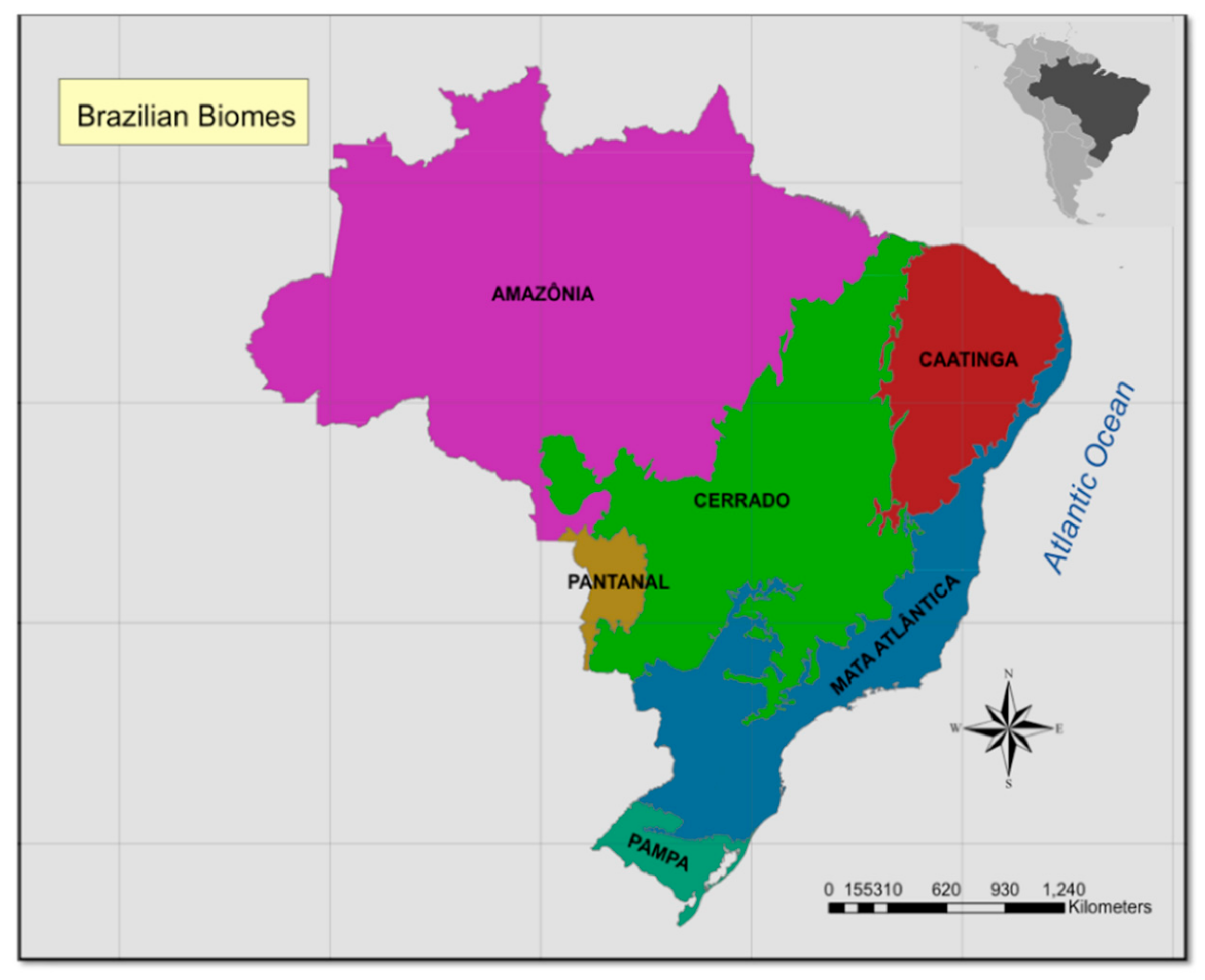
2.1. Study Areas: Brazilian Biomes

In this study, biome refers to the six main biomes of Brazil as defined by the Ministério do Meio Ambiente (MMA) as regions sharing morphoclimatic and phytogeographical characteristics: Amazon, Caatinga, Cerrado, Pampa, Pantanal, and Atlantic Forest [102]). Figure 1 shows the Brazilian biome limits utilized in this study. These biomes are used as a large spatial scale basis for comparisons of the high resolution satellite-based SIF measurements across regions for the whole country of Brazil, which covers an area of about 850 million ha [103]. Table S1 shows a list of all abbreviations used in the study.

The Amazon is the largest biome (about 50–60% of all Brazil) with a humid tropical climate, low seasonal temperature variability, approximately 1000–2000 mm of annual precipitation, containing approximately half the world’s tropical rainforest, and critical for biodiversity and the global carbon balance [84,104,105]. The Cerrado is second in area to the Amazon (about 22–25%), with about 1200–1800 mm of precipitation, experiences seasonal periods of tropical followed by dry climate, and has a great diversity of vegetation types and canopy covers, with savanna, woody savanna, dry grasslands, wet grasses, and tropical forests, often heavily fragmented for agriculture [96,97,106,107,108]. The Pantanal is one of the largest wetlands in the world (160,000 km²) with a dynamic yearly flooding regime and is a United Nations Educational, Scientific and Culture Organization (UNESCO) World Heritage site containing tropical wetlands with arid tropical species alongside dry shrubland and grasses as well as xeric species [109,110,111]. The Pantanal contains a unique hydrologic structure of seasonal inundation fed by the upper Paraguay River and average yearly rainfall of 1000–1400 mm, alternating patterns of salt and freshwater lakes (bahias and salinas), and the highest species diversity and concentration of wildlife in the world, yet it makes up only about 2% of the area of Brazil [109,110,112,113,114,115]. Despite often being referred to as a desert, the Caatinga is a semi-arid region, making up about 10% of the country, has only about 700 mm of rainfall per year, falling sometimes erratically with high temperatures and low humidity [116,117]. and the dominant vegetation is woody shrub land and savanna with abundant xerophytic species, but contains mosaics of seasonally dry tropical forests and is one of the most populated semi-arid regions of the world [96,103,116,117,118,119]. The Atlantic Forest covers a wide longitudinal area and has been heavily fragmented to only about 10% of the native vegetation remaining after once having about 150 million ha of rainforest [88,120]. The Atlantic Forest makes up about 13% of the country’s area and much of this is along the Atlantic coast having vegetation ranging from deciduous and tropical forest to mangroves and vast managed forestry plantations, other agriculture, and urban areas [88,120,121,122,123]. The average rainfall in the Atlantic forest varies greatly from coastal areas (more than 4000 mm/year) to inland (~1000 mm/year), along elevation gradients (~1600 mm/year at sea level to up to 3600 mm/year in high altitude mountain regions) and along the latitudinal expanse of the biome [120]. The Pampa is the southernmost border biome, occupies approximately 2% of Brazil, and has a transition from tropical to temperate climate, thus having four seasons, supporting grasslands and deciduous forest, and a large amount of agricultural development [124,125]. The Pampa lies within the South temperate zone with subtropical and temperate climates averaging approximately 1200–1600 mm/year precipitation [124].

2.2. Orbiting Carbon Observatory-2 (OCO-2) SIF

Launched in 2014, the Orbiting Carbon Observatory-2 (OCO-2, NASA) satellite collects SIF observations globally, offering the opportunity to measure photosynthetic activity of vegetation at higher resolution than was possible before and to employ them to address gaps in knowledge about GPP and carbon fluxes in the tropics. OCO-2 based SIF measurements provide superior spatial and spectral resolution, data acquisition techniques, and retrieval precision than previous satellite-based SIF measurements. This allows for improved validation and better determination of SIF-GPP relationships [27,44,100]. OCO-2 collects spectral data from 757 to 775 nm (the Oxygen absorption-A band; O₂A) at approximately 1330 local time (LST) allowing accurate, high resolution retrievals of instantaneous solar-induced fluorescence (SIF) within the Fraunhofer lines at 757 and 771 nm at a spectral resolution of 0.042 nm (FWHM = 0.042 nm) [44]. OCO-2 acquires 24 spectra per second producing eight cross-track spectra each covering about 2 km × 1.3 km spatial area, called a footprint, over a narrow swath width with maximum of approximately 10 km. At the Equator, the swath width narrows due to slit rotation and the instrument records spectra of only one ground footprint with all eight independent cross-track spectra [15]. The revisit period is every 16 days. Through 2 July 2015 each revisit time alternated between glint and nadir mode for the instrument, thus the repeat time for a set of nadir measurements is every 32 days. Since 2 July 2015, the instrument alternates modes for every orbit. Nadir mode measurements are recommended for studies such as this one because it follows a similar ground track each revisit time (allowing detection of temporal changes), has a higher spatial resolution, better signal-to-noise ratio and more consistent measurements under varying atmospheric conditions and topography than does glint mode [15,27,44,126,127]. OCO-2’s coverage is global, however, there are gaps between the points and swaths. Continuous spatial coverage is sacrificed for the fine spatial sampling of each OCO-2 footprint. This fine spatial sampling and high resolution SIF measurements provide the opportunity to more accurately address SIF of specific vegetation classes within and across biomes than previous satellite-based platforms used for SIF. Nonetheless, while OCO-2 SIF data have high spectral and spatial resolution, individual footprints are noisy, thus analyses in this study follow previous studies utilizing averaging in space and time [9,12,15,23,42,44,128].

The OCO-2 SIF Lite product (version 8r, “r” indicating retrospective dataset) data from September 2014–October 2017 for South America was downloaded and processed. The entire OCO-2 dataset is missing August 2017 due to the sensor not collecting during that period. The data were read in, filtered for nadir mode, and relevant variables, such as IGBP class, VPD, 2m temperature (air temperature, T_air), and skin temperature (canopy temperature, T_can) were retained for all OCO-2 footprints from the dataset. The source of these environmental variables is the European Centre for Medium-Range Weather Forecasts (ECMWF) and is included in the OCO-2 product. Brazil OCO-2 SIF footprints were co-located with shapefiles of Brazilian biomes from Ministério do Meio Ambiente (MMA, http://mapas.mma.gov.br/i3geo/datadownload.htm [102]) and all footprints in Brazil extracted and flagged for biome location. Instantaneous SIF (SIF_inst) was calculated using the average of instantaneous SIF measured at 757 nm and instantaneous SIF at 771 nm times a factor of 1.7 based on the OCO-2 Data Product User’s Guide and previous literature [15,28,126,129,130] as follows:

$$\begin{array}{c}SI{F}_{inst} = \frac{SI{F}_{757nm}+1.7SI{F}_{771nm}}{2}\end{array}$$

(1)

SIF_inst was normalized for differences in sun angle and daily changes by application of the daily mean correction factor (DCF), which is a time averaged first order approximation of a daily average SIF_d [14,126,130,131]. The DCF varies with time and latitude because these relate to the variation of the solar zenith angle (SZA) and length of the day, thus having a seasonal cycle. Although this cycle is weaker in the tropics than higher latitudes, applying the DCF to SIF is recommended for examination of seasonal cycles, comparing SIF across large spatial scales, and when examining OCO-2 based SIF to other products with different collection times [15,27,131,132].The DCF approximately accounts for the length of day and variability of the solar zenith angle (sza) using pure geometric incoming light scaling for the location in ten-minute time steps. SIF_d is calculated with the following equation

$$\begin{array}{c}{\mathrm{SIF}}_{\mathrm{d}} = \frac{{\mathrm{SIF}}_{757\mathrm{or}771\mathrm{nm}}}{\cos \left(\mathrm{sza}\left({\mathrm{t}}_{\mathrm{m}}\right)\right)}{{\displaystyle \int }}_{\mathrm{t}={\mathrm{t}}_{\mathrm{m}}-12\mathrm{h}}^{\mathrm{t}={\mathrm{t}}_{\mathrm{m}}+12\mathrm{h}}\cos \left(\mathrm{sza}\left(\mathrm{t}\right)\right)\mathrm{dt}\end{array}$$

(2)

where sza is the solar zenith angle from the OCO-2 dataset and t_m is the time of measurement [14,126,130]

The programming for downloading and processing of OCO-2 data was completed using the interactive data language (IDL; Harris Geospatial, Inc., Boulder, Co.).

2.3. Statistical Analysis for Differences in Mean SIF_d between Biomes and Vegetation Classes

The monthly average of all SIF_d observations within a biome were calculated for all vegetation classes aggregated (AVC) and an analysis of significant differences in the overall three year mean SIF_d of the biomes was performed to investigate differences in SIF_d measured among biomes. To compare the variability of SIF_d measurements among biomes, the coefficient of variation (CV) of monthly average SIF_d was calculated for each biome and an analysis of differences performed. The data were tested for normality and significant differences by examining the residuals, qq-plot, and histogram of residuals of a two-way analysis of variance (ANOVA) and post hoc testing of differences was performed using Tukey’s honestly significant difference test.

We then subset and filtered SIF_d observations in each biome for key vegetation classes based on the IGBP (Table S2, [56]): Deciduous Broadleaf Forests (DBF), Evergreen Broadleaf Forests (EBF), Grasslands (GRA), Savannas (SAV), and Woody Savannas (WSAV). The average of all SIF_d observations occurring in each month within a biome were calculated for each of the key vegetation classes. These natural (non-crop) classes composed the five largest proportions of SIF_d measurements calculated in biomes which are expected to have distinct SIF_d signals and phenological cycles. Exclusion of Open Shrublands (OSH) and Closed Shrublands (CSH), for instance, was due to the mixed deciduous and evergreen foliage contained in these classes (Table S2) in conjunction with low proportions of SIF_d measurements. To investigate differences in SIF_d measured among vegetation classes within biomes and to test for interaction between biome and vegetation class, statistical analysis of significant differences in the mean SIF_d were performed following the procedures comparing AVC SIF_d among biomes (previous paragraph). Table S3 provides the values for the distribution of OCO-2 SIF observations by biome and vegetation class for the study.

2.4. Correlation with Environmental Variables: T_can, T_air, VPD

To investigate the strength and direction of these relationships, Spearman correlations were calculated between SIF_d and the environmental variables: T_skin, T_2m, VPD for each vegetation class in each biome. All statistical analysis and figures from statistical and seasonality analysis were completed in R version 3.4.2, RStudio version 1.0.153 and the packages: dplyr, tidyverse, ggplot2, and zoo [133,134,135,136,137].

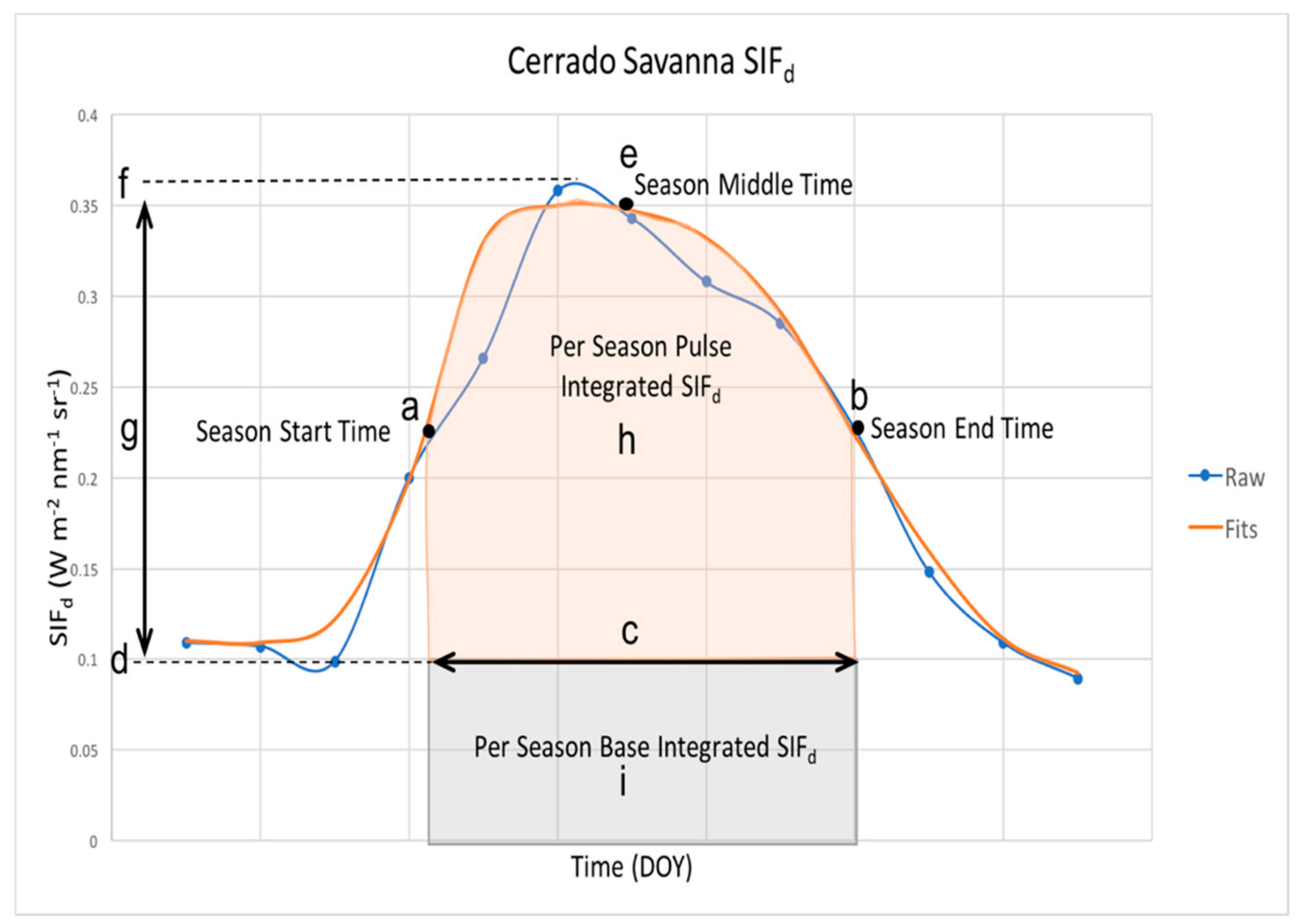
2.5. Seasonality Metrics Extraction

In order to explore the behavior that may be masked by analysis of means, especially temporal patterns, we undertook an analysis of seasonality for the vegetation classes in the biomes. We generated time series of vegetation-specific SIF_d for each biome to inspect the interannual variability of SIF_d measurements (Figure S11). Based on this inspection, we determined that the Pampa DBF data had too many missing consecutive months for the study period to be reliable. We then applied the TIMESAT algorithms to each of the other vegetation class’ SIF_d time series for each biome to calculate seasonality metrics [47,138]. TIMESAT was designed to analyze time series data from satellite sensors and generate seasonality metrics such as start of season, end of season, peak of season, season length, base value, maximum value, amplitude value, rates of increase and decrease, large (total) and small (pulse) integrals [138,139] (Figure 2). The time series of SIF_d for each vegetation class within each biome were smoothed using the median of a moving window by more than one standard deviation. After the time series were smoothed, we used the TIMESAT double logistic functions fitting method setting. The average of the seasonality metrics for seasons detected over the three-year study period (n = 2) in each time series was calculated to represent annual metrics for SIF_d seasonality of each vegetation class in each biome. A sample diagram of raw and fit data is shown in Figure 2. The algorithm determines the base as the average of the left and right minimum values, and the amplitude as the difference between the base value and the maximum (labels d and g, respectively, Figure 2). The time for begin and end of season are determined using 0.5 of the amplitude from the left and right, respectively, following methods for determining seasonality parameters in the literature [47,56,140].

From TIMESAT results, the per-season base integrated SIF_d and the pulse integrated SIF_d were analyzed to quantify annual SIF_d productivity for each vegetation class in each biome. The length of season (LOS) in days was calculated for each vegetation class in each biome. The mean LOS for a biome was calculated as the average of the SIF_d LOS of DBF, EBF, GRA, SAV and WSAV SIF_d within that biome. We examined differences in means of LOS among biomes utilizing the Kruskal Wallace test and Pairwise Wilcoxon Tests. Additionally, we used a generalized linear model (GLM) to determine if length of SIF_d season would explain the variation found in the total integrated SIF_d.

3. Results

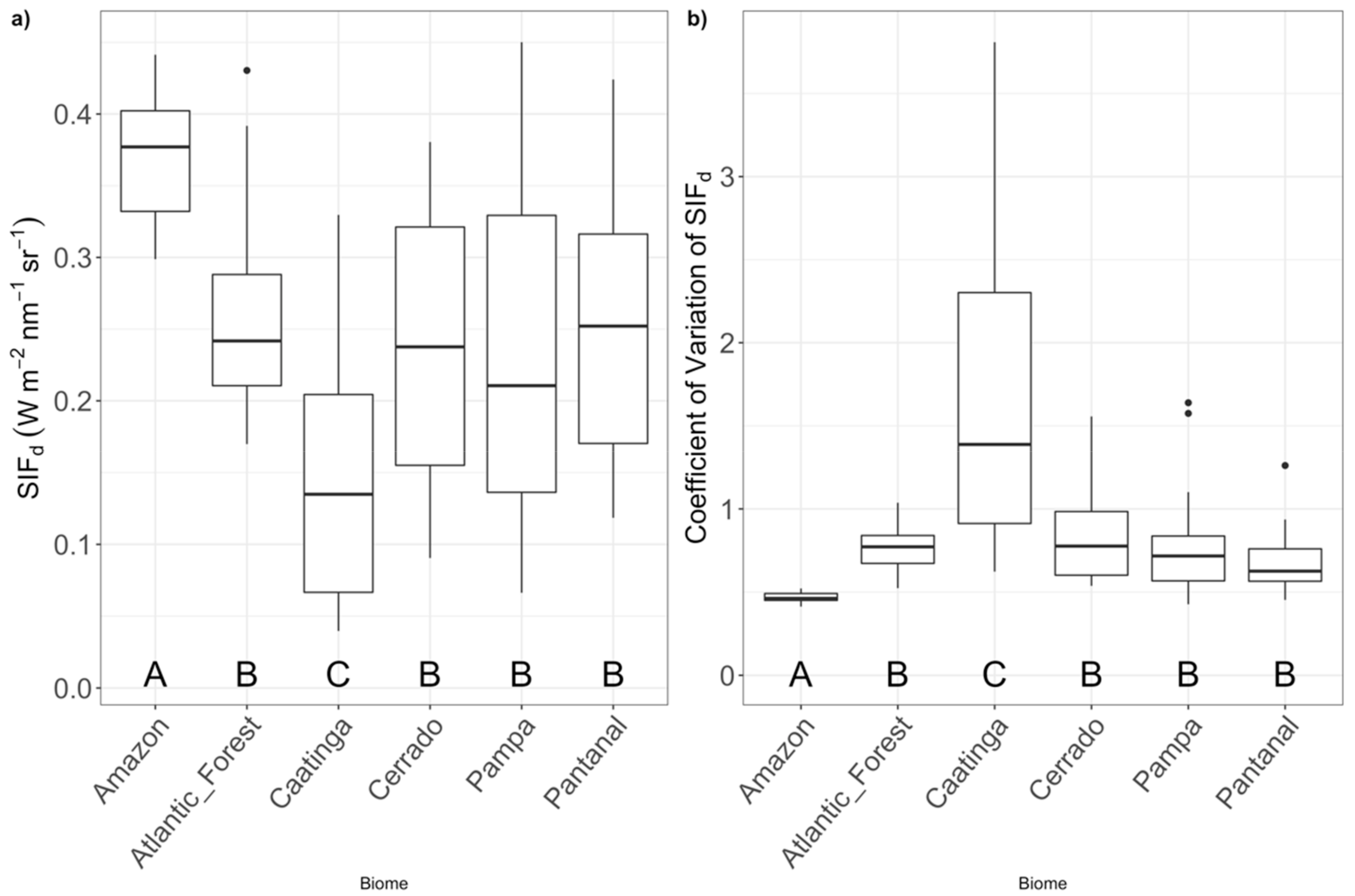
3.1. Comparison of SIF_d among Biomes

We found that Amazon AVC SIF_d is significantly different (mean = 0.38 Wm⁻²nm⁻¹sr⁻¹; Figure 3 and Table S4) than all other biomes (ANOVA, p < 0.001; Tukey’s HSD, p < 0.001; Table S5) and the Caatinga AVC SIF_d is significantly different (mean = 0.13 Wm⁻²nm⁻¹sr⁻¹; Figure 3 and Table S4) than all other biomes (ANOVA, p < 0.001; Tukey’s HSD, p < 0.001; Table S5), as might be expected based on prior understanding of biomass and chlorophyll content of vegetation in the biomes. No significant differences in AVC SIF_d were found among the Atlantic Forest (0.24 Wm⁻²nm⁻¹sr⁻¹; Figure 3 and Table S4), Cerrado (0.24 Wm⁻²nm⁻¹sr⁻¹; Figure 3 and Table S4), Pampa (0.21 Wm⁻²nm⁻¹sr⁻¹; Figure 3 and Table S4), and Pantanal (0.25 Wm⁻²nm⁻¹sr⁻¹; Figure 3 and Table S4) biomes’ AVC SIF_d. We found OCO-2 captured the lower spatial variability measured using CV of mean SIF_d in Amazon AVC SIF_d (mean CV = 0.46, p < 0.001) than all other biomes and the higher CV for the Caatinga (mean CV = 1.39, p < 0.01). No significant differences in variability of SIF_d were found among the Atlantic Forest (mean CV = 0.77), Cerrado (mean CV = 0.78), Pampa (mean CV = 0.72), and Pantanal (mean CV = 0.63) biomes. Figures S1–S7 show plots of the residuals versus fitted values, qq-plot, and histogram of residuals of the two-way ANOVA.

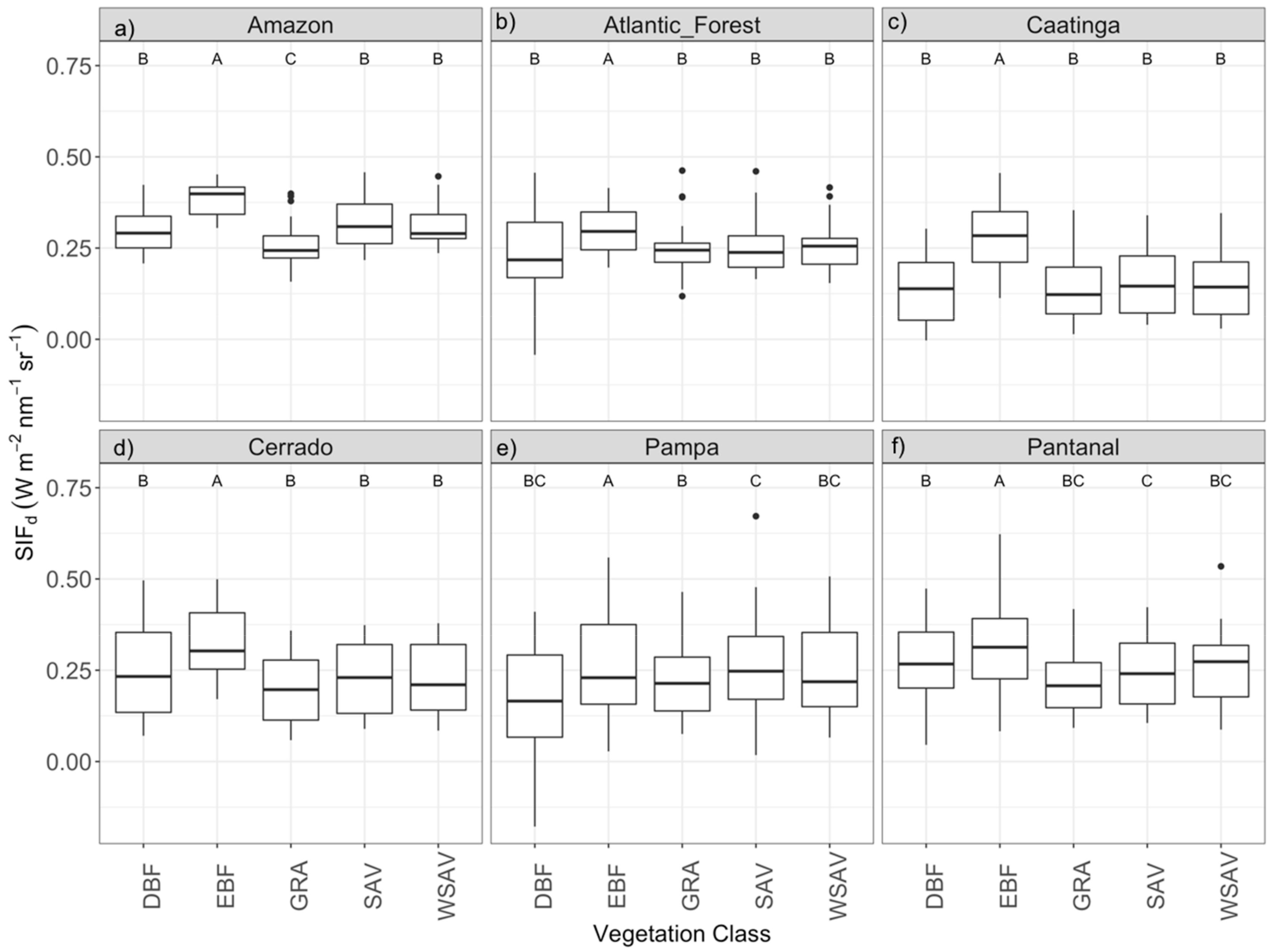
3.2. Comparison of SIF_d among Vegetation Classes within Biomes

Our analysis of mean OCO-2 SIF_d measurements distinguished forest from other classes’ SIF_d in the cases of EBF, but not DBF. In every biome, we found EBF SIF_d to be significantly different than all other vegetation classes (Tukey’s HSD, p < 0.001) Figure 4, panels a-f, Tables S4 and S6). Amazon EBF SIF_d had the highest mean of any class in any biome (mean = 0.38 Wm⁻²nm⁻¹sr⁻¹) (Figure 4, panels a–f, Tables S4 and S6). However, DBF SIF_d was not significantly different than GRA, SAV, or WSAV in any of the biomes. Among the non-forest classes, mean SIF_d analysis based on measurements from OCO-2 were partially able to distinguish GRA SIF_d from SAV SIF_d, but not able to differentiate SAV SIF_d from WSAV SIF_d. In the Amazon, GRA SIF_d was significantly lower than all other classes (mean = 0.26, p < 0.01) Figure 4 panel a Tables S4 and S6). In the Atlantic Forest, Caatinga, and Cerrado GRA SIF_d (mean = 0.25, 0.14, 0.20 Wm⁻²nm⁻¹sr⁻¹, respectively; Table S4) was not significantly different than SAV SIF_d (mean = 0.25, 0.16, 0.23 Wm⁻²nm⁻¹sr⁻¹, respectively; Table S4) but, GRA SIF_d in the Pampa and Pantanal biomes (mean = 0.23, 0.22 Wm⁻²nm⁻¹sr⁻¹, respectively; Table S4) were significantly lower than SAV SIF_d (mean = 0.27, 0.25 Wm⁻²nm⁻¹sr⁻¹, respectively; Tukey’s HSD, p < 0.05) (Figure 4, panels b–f, Tables S4 and S6). No difference was found among SAV, and WSAV SIF_d in any of the biomes. The results of a two-way ANOVA showed there was a significant interaction between biome and vegetation class on SIF_d (ANOVA F (20,1056) = 1.922). Therefore, to further investigate the comparison means of SIF_d of vegetation classes across biomes would require an exploration of the combination of biome and vegetation class as main effects.

3.3. Monthly Mean SIF_d Correlations to T_can, T_air, and VPD

In the Amazon, DBF and EBF SIF_d were not significantly correlated with T_can, T_air or VPD. The range of values for T_can, T_air, and VPD for DBF and EBF were smaller than other vegetation classes and the range of SIF_d values slightly smaller (Figures S2–S4). Amazon GRA, SAV and WSAV SIF_d were significantly negatively correlated with T_can, T_air, and VPD (r between −0.72 and −0.35, p < 0.05,

Table 1. Relationships (r values) between monthly SIF_d and T_can, T_air, and VPD for vegetation classes in each biome. p-values indicated by stars: *** = p < 0.001, ** = p < 0.01, * = p < 0.05, no stars indicate non-significant relationships.

Tcan
	Amazon	Atlantic Forest	Caatinga	Cerrado	Pampa	Pantanal
DBF SIFd	0.15	0.25	−0.51 *	−0.70 ***	0.55 **	−0.15
EBF SIFd	0.03	0.71 ***	−0.69 ***	−0.52 **	0.52 **	−0.07
GRA SIFd	−0.70 ***	−0.17	−0.82 ***	−0.58 ***	0.77 ***	−0.09
SAV SIFd	−0.35 *	0.19	−0.78 ***	−0.60 ***	0.82 ***	−0.07
WSAV SIFd	−0.41 *	0.45 **	−0.74 ***	−0.61 ***	0.83 ***	−0.04
Tair
	Amazon	Atlantic Forest	Caatinga	Cerrado	Pampa	Pantanal
DBF SIFd	0.15	0.14	−0.37 *	−0.61 ***	0.55 **	−0.13
EBF SIFd	0.03	0.74 ***	−0.57 ***	−0.50 **	0.46 **	−0.01
GRA SIFd	−0.72 ***	−0.07	−0.75 ***	−0.52 **	0.76 ***	−0.06
SAV SIFd	−0.35 *	−0.31	−0.73 ***	−0.56 ***	0.79 ***	−0.05
WSAV SIFd	−0.40 *	0.54 ***	−0.66 ***	−0.55 ***	0.82 ***	−0.02
VPD
	Amazon	Atlantic Forest	Caatinga	Cerrado	Pampa	Pantanal
DBF SIFd	0.16	0.10	−0.57 ***	−0.80 ***	0.59 **	−0.29
EBF SIFd	0.01	0.60 ***	−0.71 ***	−0.69 **	0.47 **	−0.23
GRA SIFd	−0.81 ***	−0.19	−0.85 ***	−0.72 ***	0.74 ***	−0.22
SAV SIFd	−0.60 *	0.03	−0.81 ***	−0.79 ***	0.74 ***	−0.24
WSAV SIFd	−0.55 *	0.31	−0.77 ***	−0.77 ***	0.78 ***	−0.19

* p < 0.05; ** p < 0.01; *** p < 0.001, Bolded r values greater or equal 0.70.

). Amazon GRA, SAV, and WSAV SIF_d had the strongest correlation with VPD (r = −0.81, r = −0.6, r = −0.55, respectively, p < 0.001) and less correlated with T_air (r = −0.72, r = -0.35, r = 0.40, respectively, p < 0.001) and T_can (r = −0.7, r = −0.35, r = 0.41, respectively, p < 0.001), which were similar in strength and direction with SIF_d in these classes. This indicates that variations in SIF_d are more driven by changes in VPD than to T_can or T_air. Correlations between Amazon GRA SIF_d are stronger than SAV and WSAV SIF_d (Table 1).

We found few significant relationships of vegetation class SIF_d with T_can, T_air, or VPD in the Atlantic Forest, but all those found were positive. Atlantic Forest EBF SIF_d was significantly related to T_can, T_air, and VPD (r = 0.71, 0.74, and 0.6, p < 0.001, respectively; Table 1). WSAV SIF_d was positively correlated with T_can and T_air (r = 0.45, 0.54, p < 0.001, respectively (Table 1), but not with VPD. No other correlations among SIF_d and T_can, T_air, or VPD were found in the Atlantic Forest.

In the Caatinga all vegetation classes’ SIF_d were significantly negatively correlated to T_can (r between −0.51 and −0.82, p < 0.01, Table 1) and T_air (r between −0.37 and −0.75, p < 0.05: Table 1) and with VPD (r between −0.57 and −0.85, p < 0.01; Table 1). Caatinga SIF_d in all classes (DBF, EBF, GRA, SAV, WSAV) had the strongest relationship with VPD (r = −0.57, −0.71, −0.85, −0.81, and −0.77, p < 0.001, respectively; Table 1) followed by T_can (r = −0.51 p < 0.01, r = −0.69, −0.82, −0.85, −0.78, and −0.74, p < 0.001, respectively: Table 1), then T_air (r = −0.37 p < 0.01, r = −0.57, −0.75, −0.73, and −0.66, p < 0.001, respectively; Table 1). Caatinga DBF SIF_d has the weakest correlations with T_can, T_air and VPD of the vegetation classes in the Caatinga. T_can, T_air, and VPD relationship strengths are more similar for EBF, GRA, SAV, and WSAV SIF_d in the Caatinga than for DBF and EBF SIF_d with T_can, T_air.

Relationships of vegetation class SIF_d with climatic variables are similar in the Cerrado to those in the Caatinga and the ranges of values for T_can, T_air, and VPD are more similar for the Caatinga and Cerrado than for the other biomes (Table 1, Figures S2–S4). In the Cerrado, all vegetation class’ SIF_d are significantly negatively correlated with T_can, T_air and VPD (r between −0.50 and −0.80, p < 0.01; Table 1). Correlations of Cerrado SIF_d are strongest between VPD and SIF_d (VPD: r between −0.69 and −0.80, p < 0.001: Table 1) in every vegetation class, followed by T_can (r between −0.52 and −0.70, p < 0.01), then T_air (r between −0.50 and −0.61, p < 0.01; Table 1). The Cerrado SIF_d relationships deviate from the Caatinga in that Cerrado EBF SIF_d has weaker relationships with all variables (T_can, T_air, and VPD) than the other classes’ SIF_d, while we found that DBF SIF_d had the weakest relationships with variables for all classes.

In the Pampa, all vegetation class’ SIF_d are significantly positively correlated with T_can, T_air and VPD (r between 0.46 and 0.83, p < 0.01; Table 1) in contrast to the negative correlations to T_can, T_air, and VPD found for all vegetation classes’ SIF_d in the Caatinga and Cerrado. The Pampa had the lowest maximum T_can and T_air values of any biome (311K and 308K, respectively; Figures S8 and S9) and T_can and T_air values reached lower values in the Pampa biome compared to any other biome. DBF SIF_d in the Pampa had the strongest relationship with VPD (r = 0.59, p < 0.01; Table 1) while all other vegetation classes (EBF, GRA, SAV, WSAV) were most strongly correlated with T_can (r = 0.52 p < 0.01, 0.77 p < 0.001, 0.82 p < 0.001, 0.83 p < 0.001, respectively; Table 1). EBF SIF_d in the Pampa showed the lowest correlation to VPD relative to T_can and T_air, the only vegetation class with the weakest relationship to VPD. Note the DBF sample size was the smallest of all the vegetation classes in all biomes of the study (n = 52, resulting in n = 24 for monthly average SIF_d), which may have influenced the results (Table 1).

In the Pantanal, no significant relationships were found for any vegetation class’ SIF_d with T_can, T_air, or VPD. Values of T_can and T_air were the highest and the range of VPD values was the widest in the Pantanal of all the biomes (Figures S8–S10).

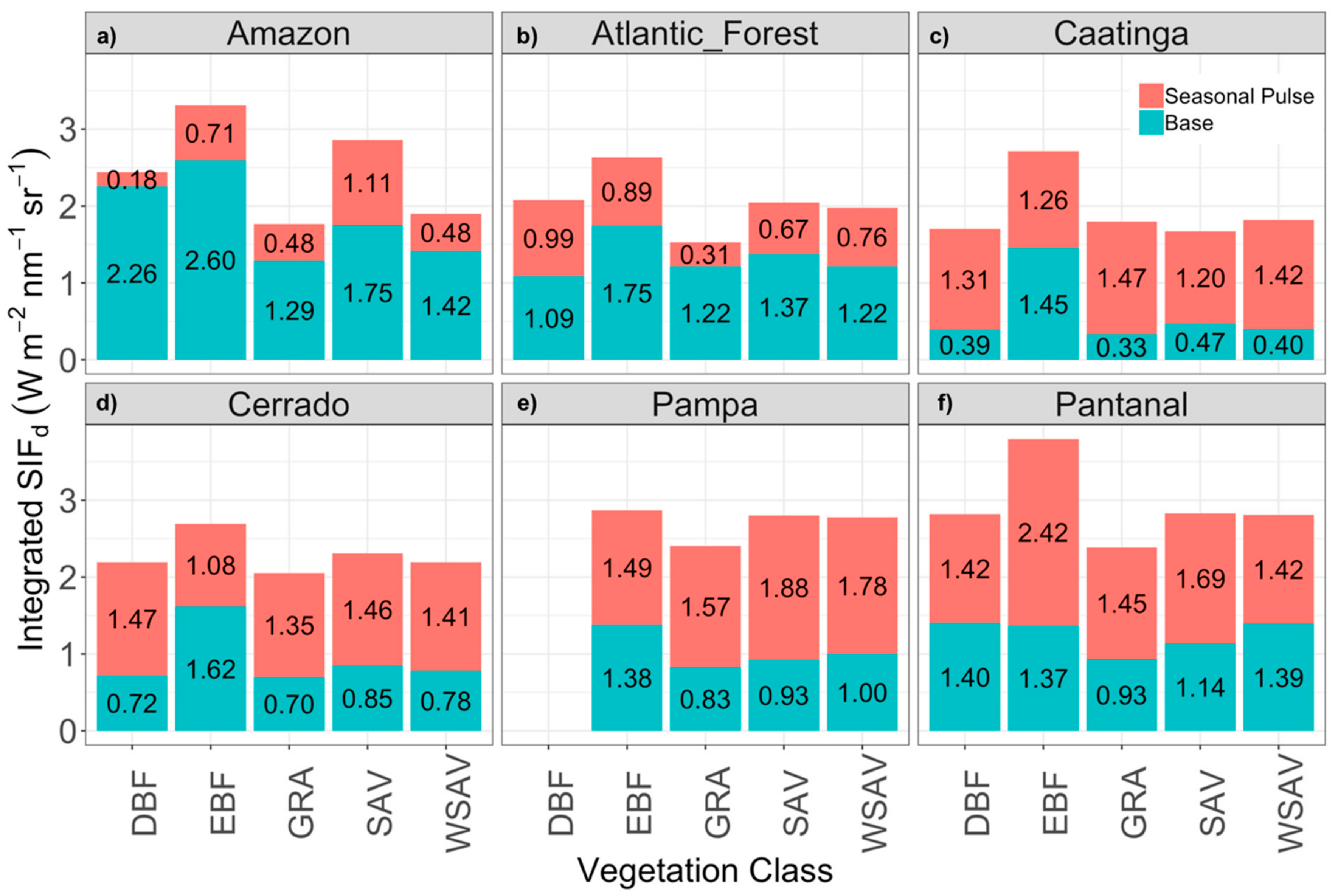
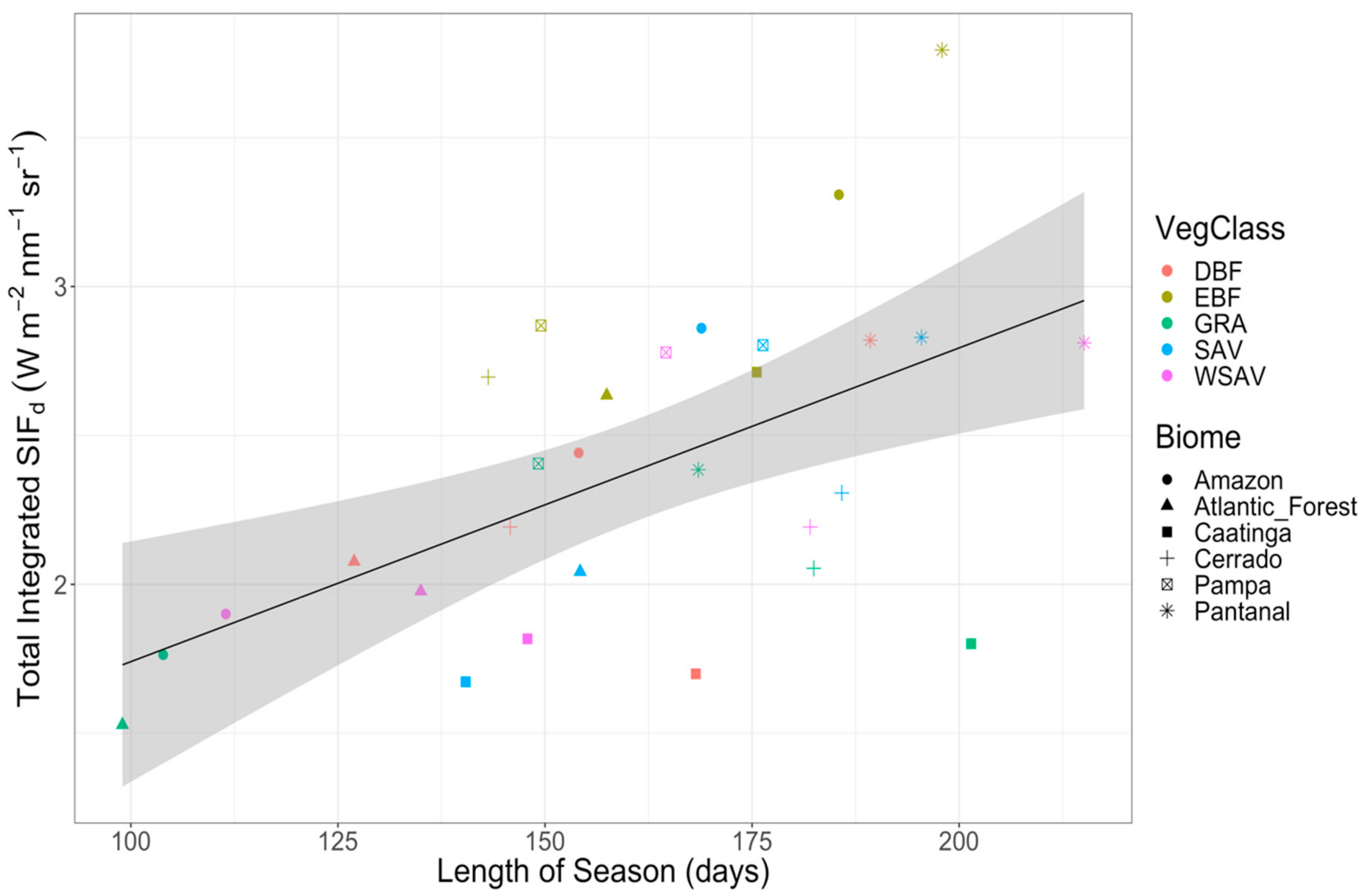
3.4. Seasonality of SIF_d

EBF SIF_d has the highest base integrated SIF_d of all vegetation classes in the Amazon as well as in any vegetation class in any other biome (2.6 Wm⁻²nm⁻¹sr⁻¹ Figure 5, panels a–f). Vegetation classes in the Amazon have higher base integrated SIF_d than their counterparts in other biomes, and generally show that the base integrated SIF_d of the Amazon, in terms of continuously high SIF_d, would be higher year-round than other biomes. Base integrated SIF_d of EBF in the Amazon exceeds all other classes in all other biomes (by 0.33 to 2.27 Wm⁻²nm⁻¹sr⁻¹). Base integrated SIF_d for GRA in the Caatinga has the lowest value of any class in any biome at 0.33 Wm⁻²nm⁻¹sr⁻¹ (Figure 5, panel c). The Amazon, Caatinga, Cerrado, and Pantanal GRA base integrated SIF_d was lower than the other than vegetation classes’ base integrated SIF_d in each of their respective biomes (1.29, 0.33, 0.7, 0.83, and 0.93 Wm⁻²nm⁻¹sr⁻¹, respectively).

The seasonal pulse integrated SIF_d values are represented as the upper bars (orange) in the stacked bar plot (Figure 5). The largest seasonal pulse SIF_d is found in the Pantanal for EBF (2.42 Wm⁻²nm⁻¹sr⁻¹). The Pampa SAV and WSAV seasonal pulse integrated SIF_d are the next larger seasonal pulse (1.88 and 1.78 Wm⁻²nm⁻¹sr⁻¹, respectively, Figure 5, panels a and e). The smallest seasonal pulses are in the Amazon and Atlantic Forest (Figure 5). Amazon DBF has the smallest seasonal pulse integrated SIF_d compared to other vegetation classes within the Amazon and across all other vegetation classes in all biomes (0.18 Wm⁻²nm⁻¹sr⁻¹) (Figure 5, panel a).

The sum of the base and seasonal pulse integrated SIF_d values represent the total seasonal integrated SIF_d (Figure 5). Total integrated SIFd of EBF exceeds all other classes in all other biomes by 0.07 to 1.10 Wm⁻²nm⁻¹sr⁻¹. When the total seasonal integrated SIF_d is considered, the Pantanal EBF integrated SIF_d has the highest overall value of 3.79 Wm⁻²nm⁻¹sr⁻¹ (Figure 5, panel f), followed closely by Amazon EBF at 3.31 Wm⁻²nm⁻¹sr⁻¹ (Figure 5, panel a), compared to all other vegetation classes in all other biomes. EBF total integrated SIF_d was the highest within each biome compared to all other vegetation classes (2.63–2.79 Wm⁻²nm⁻¹sr⁻¹, Figure 5, panel a–f). GRA total integrated SIF_d in the Atlantic Forest has the lowest value of all vegetation classes in all biomes (1.53 Wm⁻²nm⁻¹sr⁻¹, Figure 5, panel b). Within the biomes, GRA total integrated SIF_d was lowest in the Amazon (1.76 Wm⁻²nm⁻¹sr⁻¹, Figure 5, panel a), Atlantic Forest, Cerrado (2.05 Wm⁻²nm⁻¹sr⁻¹, Figure 5, panel d), and Pantanal (2.39 Wm⁻²nm⁻¹sr⁻¹, Figure 5, panel f). SAV total integrated SIF_d was the lowest value in the Caatinga (1.67 Wm⁻²nm⁻¹sr⁻¹, Figure 5, panel c).

The length of season (LOS) for each vegetation class in each biome calculated from TIMESAT showed that the values differed for vegetation classes within biomes (Figure S12). For example, Amazon EBF SIF_d LOS was the longest at 185 days and Amazon GRA SIF_d LOS was shortest at 104 days (Figure S12). Pampa WSAV has the longest calculated SIF_d LOS at 2015 days and Atlantic Forest GRA SIF_d has the shortest at 99 days (Figure S12). The mean SIF_d LOS for a biome (the average of the SIF_d LOS of DBF, EBF, GRA, SAV and WSAV within that biome) resulted in: Pantanal (193 days), Cerrado (168 days), Caatinga (167 days), Pampa (157 days), Amazon (145 days), and Atlantic Forest (135 days) (Figure S13). The only significant difference in mean SIF_d LOS was between the Pantanal and Pampa (p < 0.05), Pantanal and Atlantic Forest (p < 0.01), and the Pantanal and Amazon (p < 0.05) (Figure S13). A comparison of the SIF_d LOS of each vegetation class and the total integrated SIF_d for each vegetation class is shown in Figure 6. Our results show that the length of season only explains 30% of the variation in total integrated SIF_d (Figure 6; adjusted R² = 0.30, intercept = 0.68, slope = 0.01, p < 0.01). For every increase of one day in the length of season, on average, there is only a small corresponding increase in total integrated SIF_d of 0.01 Wm⁻²nm⁻¹sr⁻¹.

4. Discussion

Here, we compare differences in the mean and seasonal distribution of SIF_d for the country of Brazil by biome and vegetation classes within biomes. The results of our analyses and significant interaction between vegetation class and biome demonstrates that average values for vegetation classes should consider the biomes in which they occur. Furthermore, average values (Figure 4) do not capture important seasonal dynamics (Figure 5 and Figure 6), which show that high mean values can result from low rates of productivity over a longer period of time or high seasonal pulses that may be brief (Figure 5, Figures S12 and S13).

Through an examination of differences in mean and seasonality of SIF_d from satellite we were able to construct a more complete picture of vegetation photosynthetic activity of regions in Brazil as captured by OCO-2, a satellite-based instrument. In the Amazon, we found that mean SIF for the biome was highest and variation of SIF_d lowest of all other biomes, which was not surprising based on our understanding of the effects of biomass and chlorophyll content on vegetation remote sensing measurements. To our knowledge, however, no studies have previously shown these results. Mean EBF SIF_d was highest of vegetation classes within the Amazon and highest of EBF SIF in all biomes. Positive correlations between mean GRA, SAV, and WSAV SIF and T_can, T_air, and VPD were found in the Amazon and the strongest correlations were with VPD, indicating that a higher VPD is correlated with higher SIF_d for these classes. However, a lack of correlation of DBF and EBF SIF with T_can, T_air, and VPD may be attributed to the relatively small range of values for SIF, T_can, T_air, and VPD for DBF and EBF in the Amazon. Looking at seasonal metrics shows SIF_d seasonal dynamics in the Amazon that are masked by analysis of mean SIF_d. Although Amazon EBF had the highest mean SIF_d than any other vegetation class in all biomes, investigating the seasonality of SIF revealed that the Pantanal had a stronger seasonal pulse of integrated SIF_d, higher total integrated SIF_d and the longest growing season length. In contrast, Amazon forests remained productive throughout the year (based integrated SIF_d) with little seasonality (pulse integrated SIF_d). Overall, values for VPD in the Amazon were the lowest of the biomes in the study, just behind the Pampa, and T_can and T_air were relatively moderate, which indicates the most favorable photosynthetic conditions and is supported by the high rates of base integrated SIF relative to other biomes and higher base integrated SIF_d for the Amazon found in the study (Figure 5, Figures S8–S10).

For the Atlantic Forest, mean SIF_d for the biome was not different from the Cerrado, Pampa, or Pantanal. Mean EBF SIF_d was higher than other vegetation classes in the Atlantic Forest and was correlated positively with T_can, T_air, and VPD, and the strongest of these was with T_air. While mean WSAV SIF_d was not significantly different than SAV and GRA, it had a significant correlation with T_air most strongly, then with T_can next, and neither SAV nor GRA were correlated with these climate variables. This suggests that for these classes T_air is more influential compared to the other biomes. Seasonality analysis showed that EBF had the highest integrated base and total integrated SIF_d, but DBF had the highest seasonal pulse integrated SIF_d of the Atlantic Forest vegetation classes. The lack of difference in means and correlations between SIF_d and environmental variables for some vegetation classes in the Atlantic Forest may have resulted from several factors. First, the range of latitudes spanned by the Atlantic Forest biome is large (approximately 29°, ~−3° to −30°) having a corresponding large range of changes in solar angles as well as environmental conditions, the altitudinal range is large, and the Atlantic Ocean borders this latitudinal gradient, driving differences in rainfall and vegetation composition [120]. These conditions are expected to have an impact when averaging over space and time to mask trends and relationships [120,141]. Second, the degree of deforestation in the Atlantic Forest original vegetation is over 88% of the original forest and the remaining forest fragments are small (<50 ha) and isolated [120,142]. This mosaic of highly anthropogenic vegetation would make it difficult to capture the proper vegetation classification at these coarse scales and highlights the possibility that the vegetation classification may need to be improved or at higher resolution to capture vegetation class specific relationships to the environment in future studies. Third, much of the biome has been converted to cropland with asynchronous cycles of harvest and planting and it may be reasonable that croplands erroneously included in the classes examined, especially GRA and SAV, due course resolution or misclassification, would additionally affect the results and mask trends [120,142].

Investigating the biome level mean SIF_d and mean SIF_d among vegetation classes in the Caatinga only confirmed expectations, while comparisons to climate variables and analysis of seasonality further elucidated the root behavior of SIF_d in the Caatinga. Mean SIF_d of the Caatinga was lowest among all biomes, had the highest variability, and mean SIF_d among vegetation classes in the Caatinga had lower magnitudes than their counterparts in other biomes. This was anticipated based on the dry climate and vegetation makeup of dry shrubland, seasonally dry tropical forest, and xeric in contrast to other biomes [116,117]. However, correlations of mean SIF to T_can, T_air, and VPD for the Caatinga were all negative and strongest between mean SIF_d and VPD followed by T_can, just as they were in the Cerrado. This indicates mean SIF_d responds similarly in these two biomes, but in contrast to the others, potentially related to their similar latitudinal ranges and climate. Seasonality analysis revealed more intricate differences in the Caatinga. Base integrated SIF_d in the Caatinga for all vegetation classes was lowest of the biomes and seasonal pulse integrated SIF_d was not lowest, indicating that the base integrated SIF_d is responsible for the overall lower mean SIF_d (Figure 5). The lengths of individual vegetation class SIF seasons varied from those of the Cerrado (Figure S12), but the average length of the seasons for SIF in the Caatinga was not different than other biomes and was calculated within one day of the Cerrado (Figure S13). Taken together, these results support findings of previous studies showing that VPD and productivity of grasslands and seasonally dry tropical forest (measured with NDVI) vary widely and that change in climate conditions (VPD) in the wet season correlates with greater productivity [116]. However, the IGBP classification utilized in our study does not allow us to distinguish seasonally dry tropical forest or to match our results in-kind to previous studies. In order to distinguish particular vegetation class productivity behavior in future work, improved classification resolution or alignment of classification with other studies, including a seasonally dry tropical forest, would be an important component to better understand productivity in the Caatinga.

We found the Cerrado mean AVC SIF_d was not different from the Atlantic Forest, Pampa, and Pantanal at the biome level, but was different than the Caatinga and Amazon. Also, analysis of mean SIF_d among vegetation classes did not further distinguish the Cerrado. However, the Cerrado and Caatinga mean SIF_d correlations to T_can, T_air, and VPD were negative and strongest with VPD followed by T_can, in contrast to other biomes, especially the Pampa, where mean SIF_d correlations were positive and strongest with T_can. and in contrast to the Pantanal, where no significant correlations of mean SIF_d with T_can, T_air, nor VPD occurred (Table 1). These results suggest that to capture variation in vegetation function, it is necessary to investigate the individual vegetation class SIF_d in the context of climate variables because differences in the response of SIF in the Cerrado and Pampa would have been missed without investigating correlations of SIF_d with T_can, T_air, and VPD.

The Cerrado was further distinguished from the Atlantic Forest, Pampa, and Pantanal biomes by seasonality analysis of SIF_d. In the Cerrado, for instance, base integrated SIF_d is lower for all classes than Atlantic Forest, while total and pulse integrated SIF_d is higher all vegetation classes. So, year-round SIF_d in the Cerrado is less than in the Atlantic forest, but there is a higher degree of seasonality, likely driven by more pronounced cycle of environmental factors in the Cerrado versus the Atlantic Forest. Cerrado EBF base integrated SIF_d exceeds the base integrated SIF_d in the Pampa and Pantanal, but has a smaller seasonal pulse, while GRA, SAV, and WSAV SIFd in the Cerrado have lower base and seasonal pulses compared to the Pampa and Pantanal. These results indicate that the climate in the Pampa and Pantanal is more favorable to GRA, SAV, and WSAV productivity year-round and seasonally than the Cerrado, but only seasonally for EBF SIF_d. Thus, productivity of GRA, SAV, and WSAV in the Cerrado is more hindered than in the Pampa or Pantanal, likely due to the climate of the Cerrado being warmer and drier than the Pampa and drier than the Pantanal (Figure 5). In all three biomes, however, the largest values of SIF_d are captured in the EBF classes, consistent with higher biomass as expected. Furthermore, our seasonality analysis indicates the average length of season in the Cerrado is not different than any other biome (within one day of the Caatinga), but differences occur in seasonal and year-round levels of SIF_d, indicating that OCO-2 SIF captures photosynthetic activity differences. To capture subtler spatiotemporal differences, we suggest it is necessary to investigate more than differences in means based on temporal patterns that would be missed without seasonality analysis.

In the Pampa, there were no differences in mean SIF_d at the biome level with the Atlantic Forest, Cerrado, and Pantanal and analyses of mean differences in SIF among vegetation classes did not reveal any contrasts with the other biomes. However, the Pampa was unique having positive correlations with climate variables compared to other biomes, which likely result from the cooler and more temperate climate (i.e., lower values of T_can, T_air, and VPD; Figures S2–S4) in the Pampa compared to the other biomes [124]. The stark contrast of T_can and T_air ranges in the Pampa (from 286K to 311K) to the ranges in the Caatinga and Cerrado (from 297K to 319K) paired with lower VPD values in the Pampa then the Caatinga and Cerrado highlight the contrast in this Brazilian biome. The Pampa grassland dominate the vegetation and its’ phytogeography in in contrast to the biomes to its North. It is for these reasons the Pampa was expected to display different behavior, which the satellite-based SIF from OCO-2 was able to capture. It was expected that the seasonality analysis may reveal a more distinct pattern in the Pampa, such as shorter length of seasons, yet, aside from the most uniform lengths of seasons among the vegetation classes (maximum difference in length of seasons = 30), this was not the case in this study. Also unique to the Pampa biome, we showed that T_can in the Pampa is the most correlated with all vegetation classes’ SIF, except DBF. The opposite is true for DBF SIF_d, where T_can is the least correlated, however, the low number of samples of DBF in the Pampa and their lack of representation in the time series consistently make these results less reliable.

Based on mean SIF_d analysis, the Pantanal would not appear to have clear distinctions from the other biomes. No difference in biome level mean SIF_d for the Pantanal was found with the Atlantic Forest, Cerrado, and Pampa and, like other biomes mean SIF for EBF in the Pantanal was significantly higher than all other classes in the Pantanal. Yet analyses of mean SIF_d relationships to T_can, T_air, and VPD and seasonality analysis revealed important distinctions in the Pantanal. Unique to the Pantanal, we found no significant correlations with T_can, T_air, and VPD. This may be indicative of the unique patterns of evapotranspiration in this biome that is a seasonally flooded wetland, whose climate and phytogeographical distribution is unique to Brazil and the world, emphasized by its status as a UNESCO world heritage site [109,124,143]. Values of T_can, T_air and VPD for the Pantanal reach the highest values of all the biomes in the study, the mean SIF_d length of season is longer than other biomes, and vegetation class total integrated SIF_d is higher for all classes except SAV in the Pantanal compare to other biomes. Furthermore, seasonality analysis shows that total integrated SIF_d of EBF in the Pantanal exceeds total integrated SIF_d of EBF in the Amazon due to a large seasonal pulse of EBF in the Pantanal. The degree to which the total integrated SIF_d in the Pantanal exceeded the other biomes’ total integrated EBF prompted us to investigate outliers and anomalies carefully, yet none were found with these methods. These results suggest that these unique conditions give rise to vegetation responses we do not yet understand due to a lack of research in this region. To better understand SIF_d, productivity, and the climate influences on SIF_d in the Pantanal, more detailed climate and SIF_d data are needed. We suggest higher resolution SIF_d data coupled with vegetation indices, such as the photochemical reflectance index and enhanced vegetation index, measured in conjunction with temperature and precipitation, for instance.

Mean EBF SIF_d is significantly higher relative to other classes within each biome highlighting the rate of SIF_d for EBF is significantly higher in most climatic and geographic regions than its vegetation neighbors (Figure 4). These results are consistent with studies, such as Li et al. (2018), who examined OCO-2 SIF measurements and GPP from flux towers at 64 sites across the globe and found tropical forests had higher SIF in comparison with other vegetation classes [42]. However, the same study showed SIF_d in GRA was lower, while, we show mean SIF_d of GRA is not significantly different than other vegetation class mean SIF_d in four biomes (Atlantic Forest, Caatinga, Pampa, Pantanal; Figure 4) and total integrated GRA SIF_d in the Caatinga exceeds DBF and SAV total integrated SIF_d. We acknowledge, however, their study did not include data from South America and specifically examined locations with flux towers, making it difficult to compare results directly, highlighting the importance of scale and sampling location on results, and emphasizing the need for more multiscale data and research of a variety of tropical vegetation classes [42].

We examined relationships of SIF_d to T_can, T_air, and VPD, to identify potential relationships between SIF_d and the environment. Temperature is one of the most influential abiotic factors on photosynthesis and GPP, affecting physiological functioning, distribution and range shifts, and competitive success of species e.g., [4,7,8,13,140,144,145,146,147,148]. Most research has focused on T_air to examine the relationships between plant function and temperature, but recent studies have shown that T_air may not capture thermal properties of vegetation microclimate and environment. T_can has been shown to differ from T_air in that T_can is generally warmer than Tair and more coupled to water and radiative processes [140,146,149,150,151,152]. VPD influences stomatal conductance and, as such is a good metric for water stress conditions, thus lower values of VPD are generally associated with more favorable photosynthetic activity conditions for vegetation. Our results show that most biomes are most strongly related to VPD and then T_can, followed by T_air. These results support recent studies showing that T_can is potentially more related to photosynthetic function in tropical regions than T_air and serve to provide incentive to further elucidate SIF_d relationships to these variables [85,153].

We compared total integrated SIF_d to the length of season and found that the length of season explains only 30% of the variation in total integrated SIF_d (Figure 6; Adjusted R² = 0.30, m = 0.01, p < 0.001); therefore, differential physiological functioning (photosynthetic activity) responses of vegetation classes’ SIF to environmental factors are potentially more influential on the seasonal levels of SIF_d. This result is an important first step to understanding productivity of multiple tropical vegetation classes.

Our study quantifies relative SIF among vegetation classes within and across biomes. These results are most certainly also related to structure and incoming and radiation and tightly coupled to the latitude and elevation of each biome. To test and separate these factors, further study is needed at sub-biome levels fusing satellite SIF data with tower and/or unmanned aerial vehicle data on productivity for better defining the SIF-GPP relationship across scales in the tropics.

5. Conclusions

This study demonstrated that important differences in SIF_d within and across biomes can be captured and quantified with satellite SIF_d observations from OCO-2. Spatial patterns and variability investigated at biome level through statistical analyses of the observations yielded: (1) EBF SIF_d in every class had higher integrated SIF than other classes within each biome. (2) The highest mean SIF of EBF occurred in the Amazon. (3) SIF is most strongly correlated with vapor pressure deficit (VPD) for most vegetation classes in most biomes, followed by canopy temperature (T_can), although the strength and direction of the correlations depend on biome. Phenological analysis examined beyond mean differences determined that: (1) Amazon SIF_d had the highest year-round values of integrated SIF_d and the smallest seasonal pulse integrated SIF_d; (2) complex patterns of year-round and seasonal SIFd are captured by satellite measurements of SIF. (3) Pantanal EBF had the highest total integrated SIF_d due to a large seasonal pulse, and (4) the SIF_d length of season for vegetation classes only explains 30% of the variation in total integrated SIF_d; thus, the length of season is probably more closely tied to leafing patterns and leaf area, whereas integrated SIF_d captures variations in photosynthetic activity separate from structural differences. In other words, SIF and traditionally used vegetation indices may similarly define the length of seasons (vegetation indices and SIF both increase with leaf area increases), but peak season responses where traditional vegetation indices tend to saturate, are being better captured by SIF. To our knowledge, no studies have examined OCO-2 data for a comparison of vegetation class-specific SIF or phenology in the tropics. Because SIF is more mechanistically coupled to photosynthetic activity than more commonly used vegetation indices in remote sensing studies of ecosystem dynamics, our results provide novel satellite estimates of differences in productivity across biomes and vegetation types and these measurements quantify differences in SIF in continuous units (Wm⁻²nm⁻¹sr⁻¹), also in contrast to vegetation indices.

References

1. Malhi, Y. The productivity, metabolism and carbon cycle of tropical forest vegetation. J. Ecol. 2012, 100, 65–75. [Google Scholar] [CrossRef]
2. Wright, S.J. The future of tropical forests. Ann. N. Y. Acad. Sci. 2010, 1195, 1–27. [Google Scholar] [CrossRef] [PubMed]
3. Sassan, S.S.; Harris, N.L.; Brown, S.; Lefsky, M.; Mitchard, E.T.A.; Salas, W.; Zutta, B.R.; Buerman, W.; Lewis, S.L.; Hagen, S.; et al. Benchmark map of forest carbon stocks in tropical regions across three continents. Proc. Natl. Acad. Sci. USA 2011, 108, 9899–9905. [Google Scholar]
4. Wright, S.J.; Muller-Landau, H.C.; Schipper, J. The future of tropical species on a warmer planet. Conserv. Biol. 2009, 23, 1418–1426. [Google Scholar] [CrossRef] [PubMed]
5. Beer, C.; Reichstein, M.; Tomelleri, E.; Ciais, P.; Jung, M.; Carvalhais, N.; Rödenbeck, C.; Arain, M.A.; Baldocchi, D.; Bonan, G.B.; et al. Terrestrial Gross Carbon Dioxide Uptake: Global Distribution and Covariation with Climate. Science 2010, 329, 834–840. [Google Scholar] [CrossRef]
6. Huntingford, C.; Zelazowski, P.; Galbraith, D.; Mercado, L.M.; Sitch, S.; Fisher, R.; Lomas, M.; Walker, A.P.; Jones, C.D.; Booth, B.B.B.; et al. Simulated resilience of tropical rainforests to CO2-induced climate change. Nat. Geosci. 2013, 6, 268–273. [Google Scholar] [CrossRef]
7. Clark, D.A.; Asao, S.; Fisher, R.; Reed, S.; Reich, P.B.; Ryan, M.G.; Wood, T.E.; Yang, X. Reviews and syntheses: Field data to benchmark the carbon cycle models for tropical forests. Biogeosciences 2017, 14, 4663–4690. [Google Scholar] [CrossRef] [Green Version]
8. Clark, D.A.; Piper, S.C.; Keeling, C.D.; Clark, D.B. Tropical rain forest tree growth and atmospheric carbon dynamics linked to interannual temperature variation during 1984–2000. Proc. Natl. Acad. Sci. USA 2003, 100, 5852–5858. [Google Scholar] [CrossRef]
9. Joiner, J.; Yoshida, Y.; Vasilkov, A.P.; Schaefer, K.; Jung, M.; Guanter, L.; Zhang, Y.; Garrity, S.; Middleton, E.M.; Huemmrich, K.F.; et al. The seasonal cycle of satellite chlorophyll fluorescence observations and its relationship to vegetation phenology and ecosystem atmosphere carbon exchange. Remote Sens. Environ. 2014, 152, 375–391. [Google Scholar] [CrossRef] [Green Version]
10. Schimel, D.; Pavlick, R.; Fisher, J.B.; Asner, G.P.; Saatchi, S.; Townsend, P.; Miller, C.; Frankenberg, C.; Hibbard, K.; Cox, P. Observing terrestrial ecosystems and the carbon cycle from space. Glob. Chang. Biol. 2015, 21, 1762–1776. [Google Scholar] [CrossRef]
11. Rossini, M.; Nedbal, L.; Guanter, L.; Ač, A.; Alonso, L.; Burkart, A.; Cogliati, S.; Colombo, R.; Damm, A.; Drusch, M.; et al. Red and far-red sun-induced chlorophyll fluorescence as a measure of plant photosynthesis. Geophys. Res. Lett. 2015, 1632–1639. [Google Scholar] [CrossRef]
12. Guanter, L.; Zhang, Y.; Jung, M.; Joiner, J.; Voigt, M.; Berry, J.A.; Frankenberg, C.; Huete, A.R.; Zarco-Tejada, P.; Lee, J.E.; et al. Global and time-resolved monitoring of crop photosynthesis with chlorophyll fluorescence. Proc. Natl. Acad. Sci. USA 2014, 111, E1327–E1333. [Google Scholar] [CrossRef] [PubMed] [Green Version]
13. Porcar-Castell, A.; Tyystjarvi, E.; Atherton, J.; van der Tol, C.; Flexas, J.; Pfundel, E.E.; Moreno, J.; Frankenberg, C.; Berry, J.A. Linking chlorophyll a fluorescence to photosynthesis for remote sensing applications: Mechanisms and challenges. J. Exp. Bot. 2014, 65, 4065–4095. [Google Scholar] [CrossRef] [PubMed]
14. Frankenberg, C.; Fisher, J.B.; Worden, J.R.; Badgley, G.; Saatchi, S.S.; Lee, J.E.; Toon, G.C.; Butz, A.; Jung, M.; Kuze, A.; et al. New global observations of the terrestrial carbon cycle from GOSAT: Patterns of plant fluorescence with gross primary productivity. Geophys. Res. Lett. 2011, 38. [Google Scholar] [CrossRef] [Green Version]
15. Sun, Y.; Frankenberg, C.; Jung, M.; Joiner, J.; Guanter, L.; Köhler, P.; Magney, T.S. Overview of Solar-Induced chlorophyll Fluorescence (SIF) from the Orbiting Carbon Observatory-2: Retrieval, cross-mission comparison, and global monitoring for GPP. Remote Sens. Environ. 2018, 808–823. [Google Scholar] [CrossRef]
16. Joiner, J.; Yoshida, Y.; Vasilkov, A.P.; Yoshida, Y.; Corp, L.A.; Middleton, E.M. First observations of global and seasonal terrestrial chlorophyll fluorescence from space. Biogeosciences 2011, 8, 637–651. [Google Scholar] [CrossRef] [Green Version]
17. Duveiller, G.; Cescatti, A. Spatially downscaling sun-induced chlorophyll fluorescence leads to an improved temporal correlation with gross primary productivity. Remote Sens. Environ. 2016, 182, 72–89. [Google Scholar] [CrossRef]
18. Frankenberg, C. Retrieval of chlorophyll fluorescence from space. In Proceedings of the KISS Fluorescence Workshop, Jet Propulsion Laboratory/California Institute of Technology, Pasadena, CA, USA, 26–31 August 2012; pp. 1–5. [Google Scholar]
19. Meroni, M.; Rossini, M.; Guanter, L.; Alonso, L.; Rascher, U.; Colombo, R.; Moreno, J. Remote sensing of solar-induced chlorophyll fluorescence: Review of methods and applications. Remote Sens. Environ. 2009, 113, 2037–2051. [Google Scholar] [CrossRef]
20. Meroni, M.; Panigada, C.; Rossini, M.; Picchi, V.; Cogliati, S.; Colombo, R. Using optical remote sensing techniques to track the development of ozone-induced stress. Environ. Pollut. 2009, 157, 1413–1420. [Google Scholar] [CrossRef]
21. Guanter, L.; Frankenberg, C.; Dudhia, A.; Lewis, P.E.; Gómez-Dans, J.; Kuze, A.; Suto, H.; Grainger, R.G. Retrieval and global assessment of terrestrial chlorophyll fluorescence from GOSAT space measurements. Remote Sens. Environ. 2012, 121, 236–251. [Google Scholar] [CrossRef]
22. Parazoo, N.C.; Bowman, K.; Frankenberg, C.; Lee, J.-E.; Fisher, J.B.; Worden, J.; Jones, D.B.A.; Berry, J.; Collatz, G.J.; Baker, I.T.; et al. Interpreting seasonal changes in the carbon balance of southern Amazonia using measurements of XCO2and chlorophyll fluorescence from GOSAT. Geophys. Res. Lett. 2013, 40, 2829–2833. [Google Scholar] [CrossRef]
23. Wood, J.D.; Griffis, T.J.; Baker, J.M.; Frankenberg, C.; Verma, M.; Yuen, K. Multiscale analyses of solar-induced florescence and gross primary production. Geophys. Res. Lett. 2017, 44, 533–541. [Google Scholar] [CrossRef]
24. Wieneke, S.; Burkart, A.; Cendrero-Mateo, M.P.; Julitta, T.; Rossini, M.; Schickling, A.; Schmidt, M.; Rascher, U. Linking photosynthesis and sun-induced fluorescence at sub-daily to seasonal scales. Remote Sens. Environ. 2018, 219, 247–258. [Google Scholar] [CrossRef]
25. Wieneke, S.; Ahrends, H.; Damm, A.; Pinto, F.; Stadler, A.; Rossini, M.; Rascher, U. Airborne based spectroscopy of red and far-red sun-induced chlorophyll fluorescence: Implications for improved estimates of gross primary productivity. Remote Sens. Environ. 2016, 654–667. [Google Scholar] [CrossRef]
26. Damm, A.; Guanter, L.; Verhoef, W.; Schläpfer, D.; Garbari, S.; Schaepman, M.E. Impact of varying irradiance on vegetation indices and chlorophyll fluorescence derived from spectroscopy data. Remote Sens. Environ. 2015, 156, 202–215. [Google Scholar] [CrossRef]
27. Sun, Y.; Frankenberg, C.; Wood, J.D.; Schimel, D.S.; Jung, M.; Guanter, L.; Drewry, D.T.; Verma, M.; Porcar-Castell, A.; Griffis, T.J.; et al. OCO-2 advances photosynthesis observation from space via solar-induced chlorophyll fluorescence. Science 2017, 358, 5747. [Google Scholar] [CrossRef]
28. Verma, M.; Schimel, D.S.; Evans, B.; Frankenberg, C.; Beringer, J.; Drewry, D.T.; Magney, T.S.; Marang, I.; Hutley, L.; Moore, C.; et al. Effect of environmental conditions on the relationship between solar-induced fluorescence and gross primary productivity at an OzFlux grassland site. J. Geophys. Res. Biogeosci. 2017, 122, 1–18. [Google Scholar] [CrossRef]
29. Wagle, P.; Zhang, Y.; Jin, C.; Xiao, X. Comparison of solar-induced chlorophyll fluorescence, light-use efficiency, and process-based GPP models in maize. Ecol. Appl. 2016, 26, 1211–1222. [Google Scholar] [CrossRef]
30. Chen, X.; Mo, X.; Hu, S.; Liu, S. Relationship between fluorescence yield and photochemical yield under water stress and intermediate light conditions. J. Exp. Bot. 2019, 70, 301–313. [Google Scholar] [CrossRef]
31. Guan, K.; Berry, J.A.; Zhang, Y.; Joiner, J.; Guanter, L.; Badgley, G.; Lobell, D.B. Improving the monitoring of crop productivity using spaceborne solar-induced fluorescence. Glob. Chang. Biol. 2016, 22, 716–726. [Google Scholar] [CrossRef]
32. Panigada, C.; Rossini, M.; Meroni, M.; Cilia, C.; Busetto, L.; Amaducci, S.; Boschetti, M.; Cogliati, S.; Picchi, V.; Pinto, F.; et al. Fluorescence, PRI and canopy temperature for water stress detection in cereal crops. Int. J. Appl. Earth Obs. Geoinf. 2014, 30, 167–178. [Google Scholar] [CrossRef]
33. Moreno, J.; Moran, S. Vegetation stress from soil moisture and chlorophyll fluorescence: Synergy between SMAP and FLEX approaches. In Proceedings of the EGU General Assembly Conference Abstracts, Vienna, Austria, 27 April–2 May 2014; p. 10574. [Google Scholar]
34. Van Wittenberghe, S.; Alonso, L.; Verrelst, J.; Hermans, I.; Delegido, J.; Veroustraete, F.; Valcke, R.; Moreno, J.; Samson, R. Upward and downward solar-induced chlorophyll fluorescence yield indices of four tree species as indicators of traffic pollution in Valencia. Environ. Pollut. 2013, 173, 29–37. [Google Scholar] [CrossRef] [PubMed]
35. Lee, J.E.; Frankenberg, C.; van der Tol, C.; Berry, J.A.; Guanter, L.; Boyce, C.K.; Fisher, J.B.; Morrow, E.; Worden, J.R.; Asefi, S.; et al. Forest productivity and water stress in Amazonia: Observations from GOSAT chlorophyll fluorescence. Proc. Biol. Sci. R. Soc. 2013, 280, 20130171. [Google Scholar] [CrossRef] [PubMed]
36. Zarco-Tejada, P.J.; González-Dugo, V.; Berni, J.A.J. Fluorescence, temperature and narrow-band indices acquired from a UAV platform for water stress detection using a micro-hyperspectral imager and a thermal camera. Remote Sens. Environ. 2012, 117, 322–337. [Google Scholar] [CrossRef]
37. Zarco-Tejada, P.J.; Berni, J.A.J.; Suárez, L.; Sepulcre-Cantó, G.; Morales, F.; Miller, J.R. Imaging chlorophyll fluorescence with an airborne narrow-band multispectral camera for vegetation stress detection. Remote Sens. Environ. 2009, 113, 1262–1275. [Google Scholar] [CrossRef]
38. Migliavacca, M.; Perez-Priego, O.; Rossini, M.; El-Madany, T.S.; Moreno, G.; van der Tol, C.; Rascher, U.; Berninger, A.; Bessenbacher, V.; Burkart, A.; et al. Plant functional traits and canopy structure control the relationship between photosynthetic CO2 uptake and far-red sun-induced fluorescence in a Mediterranean grassland under different nutrient availability. New Phytol. 2017, 1078–1091. [Google Scholar] [CrossRef] [PubMed]
39. Yang, X.; Tang, J.; Mustard, J.F.; Lee, J.E.; Rossini, M.; Joiner, J.; Munger, J.W.; Kornfeld, A.; Richardson, A.D. Solar-induced chlorophyll fluorescence that correlates with canopy photosynthesis on diurnal and seasonal scales in a temperate deciduous forest. Geophys. Res. Lett. 2015, 2977–2987. [Google Scholar] [CrossRef]
40. Walther, S.; Voigt, M.; Thum, T.; Gonsamo, A.; Zhang, Y.; Koehler, P.; Jung, M.; Varlagin, A.; Guanter, L. Satellite chlorophyll fluorescence measurements reveal large-scale decoupling of photosynthesis and greenness dynamics in boreal evergreen forests. Glob. Chang. Biol. 2015, 2979–2996. [Google Scholar] [CrossRef]
41. Li, X.; Xiao, J.; He, B. Higher absorbed solar radiation partly offset the negative effects of water stress on the photosynthesis of Amazon forests during the 2015 drought. Environ. Res. Lett. 2018, 044005. [Google Scholar] [CrossRef]
42. Li, X.; Xiao, J.; He, B.; Altaf Arain, A.M.; Beringer, J.; Desai, A.R.; Emmel, C.; Hollinger, D.Y.; Krasnova, A.; Mammarella, I.; et al. Solar-induced chlorophyll fluorescence is strongly correlated with terrestrial photosynthesis for a wide variety of biomes: First global analysis based on OCO-2 and flux tower observations. Glob. Chang. Biol. 2018, 3990–4008. [Google Scholar] [CrossRef]
43. Zarco-Tejada, P.J.; Morales, A.; Testi, L.; Villalobos, F.J. Spatio-temporal patterns of chlorophyll fluorescence and physiological and structural indices acquired from hyperspectral imagery as compared with carbon fluxes measured with eddy covariance. Remote Sens. Environ. 2013, 133, 102–115. [Google Scholar] [CrossRef]
44. Frankenberg, C.; O’Dell, C.; Berry, J.; Joiner, J.; Köhler, P.; Pollock, R.; Taylor, T.E. Prospects for chlorophyll fluorescence remote sensing from the Orbiting Carbon Observatory-2. Remote Sens. Environ. 2014, 147, 1–12. [Google Scholar] [CrossRef] [Green Version]
45. Damm, A.; Elbers, J.; Erler, A.; Gioli, B.; Hamdi, K.; Hutjes, R.; Kosvancova, M.; Meroni, M.; Miglietta, F.; Moersch, A.; et al. Remote sensing of sun-induced fluorescence to improve modeling of diurnal courses of gross primary production (GPP). Glob. Chang. Biol. 2010, 16, 171–186. [Google Scholar] [CrossRef]
46. Cox, P.M.; Pearson, D.; Booth, B.B.; Friedlingstein, P.; Huntingford, C.; Jones, C.D.; Luke, C.M. Sensitivity of tropical carbon to climate change constrained by carbon dioxide variability. Nature 2013, 494, 341–344. [Google Scholar] [CrossRef] [PubMed]
47. Xu, L.; Saatchi, S.S.; Yang, Y.; Myneni, R.B.; Frankenberg, C.; Chowdhury, D.; Bi, J. Satellite observation of tropical forest seasonality: Spatial patterns of carbon exchange in Amazonia. Environ. Res. Lett. 2015, 10, 084005. [Google Scholar] [CrossRef]
48. Xiao, X.; Hagen, S.; Zhang, Q.; Keller, M.; Moore, B. Detecting leaf phenology of seasonally moist tropical forests in South America with multi-temporal MODIS images. Remote Sens. Environ. 2006, 103, 465–473. [Google Scholar] [CrossRef]
49. Jones, M.O.; Kimball, J.S.; Nemani, R.R. Asynchronous Amazon forest canopy phenology indicates adaptation to both water and light availability. Environ. Res. Lett. 2014, 9, 124021. [Google Scholar] [CrossRef]
50. Ma, J.; Xiao, X.; Zhang, Y.; Doughty, R.; Chen, B.; Zhao, B. Spatial-temporal consistency between gross primary productivity and solar-induced chlorophyll fluorescence of vegetation in China during 2007–2014. Sci. Total Environ. 2018, 639, 1241–1253. [Google Scholar] [CrossRef]
51. Lu, X.; Cheng, X.; Li, X.; Chen, J.; Sun, M.; Ji, M.; He, H.; Wang, S.; Li, S.; Tang, J. Seasonal patterns of canopy photosynthesis captured by remotely sensed sun-induced fluorescence and vegetation indexes in mid-to-high latitude forests: A cross-platform comparison. Sci. Total Environ. 2018, 644, 439–451. [Google Scholar] [CrossRef]
52. Springer, K.; Wang, R.; Gamon, J.A. Parallel Seasonal Patterns of Photosynthesis, Fluorescence, and Reflectance Indices in Boreal Trees. Remote Sens. 2017, 9, 691. [Google Scholar] [CrossRef]
53. Yang, H.; Yang, X.; Zhang, Y.; Heskel, M.A.; Lu, X.; Munger, J.W.; Sun, S.; Tang, J. Chlorophyll fluorescence tracks seasonal variations of photosynthesis from leaf to canopy in a temperate forest. Glob. Chang. Biol. 2017, 23, 2874–2886. [Google Scholar] [CrossRef] [PubMed]
54. Zarco-Tejada, P.J.; González-Dugo, M.V.; Fereres, E. Seasonal stability of chlorophyll fluorescence quantified from airborne hyperspectral imagery as an indicator of net photosynthesis in the context of precision agriculture. Remote Sens. Environ. 2016, 179, 89–103. [Google Scholar] [CrossRef]
55. Jeong, S.-J.; Ho, C.-H.; Gim, H.-J.; Brown, M.E. Phenology shifts at start vs. end of growing season in temperate vegetation over the Northern Hemisphere for the period 1982–2008. Glob. Chang. Biol. 2011, 17, 2385–2399. [Google Scholar] [CrossRef]
56. Zhang, X.; Friedl, M.A.; Schaaf, C.B.; Strahler, A.H.; Hodges, J.C.F. Monitoring vegetation phenology using MODIS. Remote Sens. Environ. 2003, 84, 471–476. [Google Scholar] [CrossRef]
57. Gu, L.; Baldocci, D.D.; Wofsy, S.C.; Munger, J.W.; Michalsky, J.J.; Urbanski, S.P.; Boden, T.A. Response of a Deciduous Forest to the Mount Pinatubo Eruption: Enhanced Photosynthesis. Science 2003, 299, 2035–2038. [Google Scholar] [CrossRef] [PubMed] [Green Version]
58. Wright, S.J.; Calderón, O.; Muller-Landau, H.C. A phenology model for tropical species that flower multiple times each year. Ecol. Res. 2019, 34, 20–29. [Google Scholar] [CrossRef]
59. Wu, C.; Gonsamo, A.; Gough, C.M.; Chen, J.M.; Xu, S. Modeling growing season phenology in North American forests using seasonal mean vegetation indices from MODIS. Remote Sens. Environ. 2014, 147, 79–88. [Google Scholar] [CrossRef]
60. Yang, J.; Tian, H.; Pan, S.; Chen, G.; Zhang, B.; Dangal, S. Amazon droughts and forest responses: Largely reduced forest photosynthesis but slightly increased canopy greenness during the extreme drought of 2015/2016. Glob. Chang. Biol. 2018, 1919–1934. [Google Scholar] [CrossRef]
61. Guan, K.; Pan, M.; Li, H.; Wolf, A.; Wu, J.; Medvigy, D.; Caylor, K.K.; Sheffield, J.; Wood, E.F.; Malhi, Y.; et al. Photosynthetic seasonality of global tropical forests constrained by hydroclimate. Nat. Geosci. 2015, 8, 284–289. [Google Scholar] [CrossRef]
62. Lewis, S.L. Tropical forests and the changing earth system. Philos. Trans. R. Soc. Lond. Ser. B Biol. Sci. 2006, 361, 195–210. [Google Scholar] [CrossRef]
63. Huete, A.R.; Didan, K.; Shimabukuro, Y.E.; Ratana, P.; Saleska, S.R.; Hutyra, L.R.; Yang, W.; Nemani, R.R.; Myneni, R. Amazon rainforests green-up with sunlight in dry season. Geophys. Res. Lett. 2006, 33. [Google Scholar] [CrossRef] [Green Version]
64. Samanta, A.; Knyazikhin, Y.; Xu, L.; Dickinson, R.E.; Fu, R.; Costa, M.H.; Saatchi, S.S.; Nemani, R.R.; Myneni, R.B. Seasonal changes in leaf area of Amazon forests from leaf flushing and abscission. J. Geophys. Res. Biogeosci. 2012, 117. [Google Scholar] [CrossRef] [Green Version]
65. Myneni, R.B.; Yang, W.; Nemani, R.R.; Huete, A.R.; Dickinson, R.E.; Knyazikhin, Y.; Didan, K.; Fu, R.; Negron Juarez, R.I.; Saatchi, S.S.; et al. Large seasonal swings in leaf area of Amazon rainforests. Proc. Natl. Acad. Sci. USA 2007, 104, 4820–4823. [Google Scholar] [CrossRef] [PubMed] [Green Version]
66. Morton, D.C.; Rubio, J.; Cook, B.D.; Gastellu-Etchegorry, J.P.; Longo, M.; Choi, H.; Hunter, M.O.; Keller, M. Amazon forest structure generates diurnal and seasonal variability in light utilization. Biogeosci. Discuss. 2015, 12, 19043–19072. [Google Scholar] [CrossRef]
67. Morton, D.C.; Nagol, J.; Carabajal, C.C.; Rosette, J.; Palace, M.; Cook, B.D.; Vermote, E.F.; Harding, D.J.; North, P.R. Amazon forests maintain consistent canopy structure and greenness during the dry season. Nature 2014, 506, 221–224. [Google Scholar] [CrossRef] [PubMed]
68. Samanta, A.; Ganguly, S.; Vermote, E.; Nemani, R.R.; Myneni, R.B. Why Is Remote Sensing of Amazon Forest Greenness So Challenging? Earth Interact. 2012, 16, 1–14. [Google Scholar] [CrossRef] [Green Version]
69. Quentin, G.R. Interactions of Vegetation and Climate: Remote Observations, Earth System Models, and the Amazon For; University of Washington: Seattle, WA, USA, 2018. [Google Scholar]
70. Li, X.; Xiao, J.; He, B. Chlorophyll fluorescence observed by OCO-2 is strongly related to gross primary productivity estimated from flux towers in temperate forests. Remote Sens. Environ. 2018, 204, 659–671. [Google Scholar] [CrossRef]
71. Liu, L.; Liu, X.; Hu, J. Effects of spectral resolution and SNR on the vegetation solar-induced fluorescence retrieval using FLD-based methods at canopy level. Eur. J. Remote Sens. 2015, 48, 742–761. [Google Scholar] [CrossRef]
72. Sims, D.; Rahman, A.; Cordova, V.; Elmasri, B.; Baldocchi, D.; Bolstad, P.; Flanagan, L.; Goldstein, A.; Hollinger, D.; Misson, L. A new model of gross primary productivity for North American ecosystems based solely on the enhanced vegetation index and land surface temperature from MODIS. Remote Sens. Environ. 2008, 112, 1633–1646. [Google Scholar] [CrossRef]
73. Heinsch, F.A.; Maosheng, Z.; Running, S.W.; Kimball, J.S.; Nemani, R.R.; Davis, K.J.; Bolstad, P.V.; Cook, B.D.; Desai, A.R.; Ricciuto, D.M.; et al. Evaluation of remote sensing based terrestrial productivity from MODIS using regional tower eddy flux network observations. IEEE Trans. Geosci. Remote Sens. 2006, 44, 1908–1925. [Google Scholar] [CrossRef] [Green Version]
74. Running, S.W.; Zhao, M.Z. User’s Guide Daily GPP and Annual NPP (MOD17A2/A3) Products NASA Earth Observing System MODIS Land Algorithm. Available online: https://bit.ly/2Zai7qo (accessed on 23 July 2019).
75. MODIS-Derived Terrestrial Primary Production. Available online: https://0-link-springer-com.brum.beds.ac.uk/chapter/10.1007/978-1-4419-6749-7_28 (accessed on 23 July 2019).
76. Running, S.W.; Nemani, R.R.; Heinsch, F.A.; Zhao, M.; Reeves, M.; Hashimoto, H. A Continuous Satellite-Derived Measure of Global Terrestrial Primary Production. BioScience 2004, 54, 547–551. [Google Scholar] [CrossRef]
77. Wu, J.; Guan, K.; Hayek, M.; Restrepo-Coupe, N.; Wiedemann, K.T.; Xu, X.; Wehr, R.; Christoffersen, B.O.; Miao, G.; da Silva, R.; et al. Partitioning controls on Amazon forest photosynthesis between environmental and biotic factors at hourly to interannual timescales. Glob. Chang. Biol. 2017, 23, 1240–1257. [Google Scholar] [CrossRef] [PubMed]
78. Paul-Limoges, E.; Damm, A.; Hueni, A.; Liebisch, F.; Eugster, W.; Schaepman, M.E.; Buchmann, N. Effect of environmental conditions on sun-induced fluorescence in a mixed forest and a cropland. Remote Sens. Environ. 2018, 219, 310–323. [Google Scholar] [CrossRef]
79. Atherton, J.; Nichol, C.J.; Porcar-Castell, A. Using spectral chlorophyll fluorescence and the photochemical reflectance index to predict physiological dynamics. Remote Sens. Environ. 2016, 176, 17–30. [Google Scholar] [CrossRef]
80. Biudes, M.S.; Vourlitis, G.L.; Machado, N.G.; de Arruda, P.H.Z.; Neves, G.A.R.; de Almeida Lobo, F.; Neale, C.M.U.; Nogueira, J.S. Patterns of energy exchange for tropical ecosystems across a climategradient in Mato Grosso, Brazil. Agric. For. Meteorol. 2015, 202, 13. [Google Scholar] [CrossRef]
81. Liu, X.; Chen, X.; Li, R.; Long, F.; Zhang, L.; Zhang, Q.; Li, J. Water-use efficiency of an old-growth forest in lower subtropical China. Sci. Rep. 2017, 7, 42761. [Google Scholar] [CrossRef] [PubMed]
82. Lu, X.; Liu, Z.; An, S.; Miralles, D.G.; Maes, W.; Liu, Y.; Tang, J. Potential of solar-induced chlorophyll fluorescence to estimate transpiration in a temperate forest. Agric. For. Meteorol. 2018, 252, 75–87. [Google Scholar] [CrossRef]
83. Lewis, S.L.; Brando, P.M.; Phillips, O.L.; van der Heijden, G.M.; Nepstad, D. The 2010 Amazon drought. Science 2011, 331, 554. [Google Scholar] [CrossRef]
84. Phillips, O.L.; Aragão, L.E.O.C.; Lewis, S.L.; Fisher, J.B.; Lloyd, J.; López-González, G.; Malhi, Y.; Monteagudo, A.; Peacock, J.; Carlos, A.; et al. Quesada. Drought sensitivity of the Amazon rainforest. Science 2009, 323, 1344–1348. [Google Scholar] [CrossRef]
85. Pau, S.; Detto, M.; Kim, Y.; Still, C.J. Tropical forest temperature thresholds for gross primary productivity. Ecosphere 2018, 9, 1–13. [Google Scholar] [CrossRef]
86. Moreira de Araújo, F.; Ferreira, L.G.; Arantes, A.E. Distribution Patterns of Burned Areas in the Brazilian Biomes: An Analysis Based on Satellite Data for the 2002–2010 Period. Remote Sens. 2012, 4, 1929–1946. [Google Scholar] [CrossRef]
87. Laurance, W.F.; Useche, D.C.; Rendeiro, J.; Kalka, M.; Bradshaw, C.J.; Sloan, S.P.; Laurance, S.G.; Campbell, M.; Abernethy, K.; Alvarez, P.; et al. Averting biodiversity collapse in tropical forest protected areas. Nature 2012, 489, 290–294. [Google Scholar] [CrossRef] [PubMed] [Green Version]
88. Putz, S.; Groeneveld, J.; Henle, K.; Knogge, C.; Martensen, A.C.; Metz, M.; Metzger, J.P.; Ribeiro, M.C.; de Paula, M.D.; Huth, A. Long-term carbon loss in fragmented Neotropical forests. Nat. Commun. 2014, 5, 5037. [Google Scholar] [CrossRef] [PubMed] [Green Version]
89. Giulietti, A.M.; Harley, R.M.; De Queiroz, L.P.; Van Den Berg, C. Biodiversity and Conservation of Plants in Brazil. Conserv. Biol. 2005, 19, 632–640. [Google Scholar] [CrossRef]
90. Schwieder, M.; Leitão, P.J.; da Cunha Bustamante, M.M.; Ferreira, L.G.; Rabe, A.; Hostert, P. Mapping Brazilian savanna vegetation gradients with Landsat time series. Int. J. Appl. Earth Obs. Geoinf. 2016, 52, 361–370. [Google Scholar] [CrossRef]
91. Abreu, R.C.R.; Hoffmann, W.A.; Vasconcelos, H.L.; Pilon, N.A.; Rossatto, D.R.; Durigan, G. The biodiversity cost of carbon sequestration in tropical savanna. Sci. Adv. 2017, 3, 7. [Google Scholar] [CrossRef] [PubMed]
92. Murphy, B.P.; Andersen, A.N.; Parr, C.L. The underestimated biodiversity of tropical grassy biomes. Philos. Trans. R. Soc. Lond. Ser. B Biol. Sci. 2016, 371. [Google Scholar] [CrossRef]
93. Parr, C.L.; Lehmann, C.E.; Bond, W.J.; Hoffmann, W.A.; Andersen, A.N. Tropical grassy biomes: Misunderstood, neglected, and under threat. Trends Ecol. Evol. 2014, 29, 205–213. [Google Scholar] [CrossRef]
94. John Grace, J.; San José, J.; Meir, P.; Miranda, H.S.; Montes, R.A. Productivity and carbon fluxes of tropicalsavannas. J. Biogeogr. 2006, 33, 14. [Google Scholar]
95. Ferreira, L.; Fernandez, L.; Sano, E.; Field, C.; Sousa, S.; Arantes, A.; Araújo, F. Biophysical Properties of Cultivated Pastures in the Brazilian Savanna Biome: An Analysis in the Spatial-Temporal Domains Based on Ground and Satellite Data. Remote Sens. 2013, 5, 307–326. [Google Scholar] [CrossRef] [Green Version]
96. Beuchle, R.; Grecchi, R.C.; Shimabukuro, Y.E.; Seliger, R.; Eva, H.D.; Sano, E.; Achard, F. Land cover changes in the Brazilian Cerrado and Caatinga biomes from 1990 to 2010 based on a systematic remote sensing sampling approach. Appl. Geogr. 2015, 58, 116–127. [Google Scholar] [CrossRef]
97. Alvarado, S.T.; Fornazari, T.; Cóstola, A.; Morellato, L.P.C.; Silva, T.S.F. Drivers of fire occurrence in a mountainous Brazilian cerrado savanna: Tracking long-term fire regimes using remote sensing. Ecol. Indic. 2017, 78, 270–281. [Google Scholar] [CrossRef] [Green Version]
98. Hoekstra, J.M.; Boucher, T.M.; Ricketts, T.H.; Roberts, C. Confronting a biome crisis: Global disparities of habitat loss and protection. Ecol. Lett. 2005, 8, 7. [Google Scholar] [CrossRef]
99. Zhang, Y.; Joiner, J.; Gentine, P.; Zhou, S. Reduced solar-induced chlorophyll fluorescence from GOME-2 during Amazon drought caused by dataset artifacts. Glob. Chang. Biol. 2018, 2229–2230. [Google Scholar] [CrossRef] [PubMed]
100. Köhler, P.; Guanter, L.; Kobayashi, H.; Walther, S.; Yang, W. Assessing the potential of sun-induced fluorescence and the canopy scattering coefficient to track large-scale vegetation dynamics in Amazon forests. Remote Sens. Environ. 2017, 769–785. [Google Scholar] [CrossRef]
101. SIF, STRESS, and GPP in Amazonia. Available online: https://ocov2.jpl.nasa.gov/files/ocov2/Baker-2018Aug143.pdf (accessed on 23 July 2019).
102. Ministério do Meio Ambiente. Available online: http://www.mma.gov.br (accessed on 23 July 2019).
103. Nogueira, J.; Rambal, S.; Barbosa, J.; Mouillot, F. Spatial Pattern of the Seasonal Drought/Burned Area Relationship across Brazilian Biomes: Sensitivity to Drought Metrics and Global Remote-Sensing Fire Products. Climate 2017, 5, 42. [Google Scholar] [CrossRef]
104. Malhi, J.; Roberts, J.T.; Betts, R.A.; Killeen, T.J.; Li, W.; Nobre, C.A. Climate Change, Deforestation, and the Fate of the Amazon. Science 2008, 319, 169–174. [Google Scholar] [CrossRef]
105. Hilker, T.; Lyapustin, A.I.; Hall, F.G.; Myneni, R.; Knyazikhin, Y.; Wang, Y.; Sellers, P.J. On the measurability of change in Amazon vegetation from MODIS. Remote Sens. Environ. 2015, 166, 233–242. [Google Scholar] [CrossRef]
106. Grecchi, R.C.; Gwyn, Q.H.J.; Bénié, G.B.; Formaggio, A.R.; Fahl, F.C. Land use and land cover changes in the Brazilian Cerrado: A multidisciplinary approach to assess the impacts of agricultural expansion. Appl. Geogr. 2014, 55, 300–312. [Google Scholar] [CrossRef]
107. Reynolds, J.; Wesson, K.; Desbiez, A.; Ochoa-Quintero, J.; Leimgruber, P. Using Remote Sensing and Random Forest to Assess the Conservation Status of Critical Cerrado Habitats in Mato Grosso do Sul, Brazil. Land 2016, 5, 12. [Google Scholar] [CrossRef]
108. Arantes, A.E.; Ferreira, L.G.; Coe, M.T. The seasonal carbon and water balances of the Cerrado environment of Brazil: Past, present, and future influences of land cover and land use. ISPRS J. Photogramm. Remote Sens. 2016, 117, 66–78. [Google Scholar] [CrossRef]
109. Junk, W.J.; da Cunha, C.N.; Wantzen, K.M.; Petermann, P.; Strüssmann, C.; Marques, M.I.; Adis, J. Biodiversity and its conservation in the Pantanal of Mato Grosso, Brazil. Aquat. Sci. 2006, 68, 278–309. [Google Scholar] [CrossRef]
110. Assine, M.L.; Corradini, F.A.; Pupim, F.d.N.; McGlue, M.M. Channel arrangements and depositional styles in the São Lourenço fluvial megafan, Brazilian Pantanal wetland. Sediment. Geol. 2014, 301, 172–184. [Google Scholar] [CrossRef]
111. Costa, M.; Telmer, K.H.; Evans, T.L.; Almeida, T.I.R.; Diakun, M.T. The lakes of the Pantanal: Inventory, distribution, geochemistry, and surrounding landscape. Wetl. Ecol. Manag. 2015, 23, 19–39. [Google Scholar] [CrossRef]
112. Hellman, F. Modeling Land Use Change in the Pantanal; Wageningen University: Wageningen, The Netherlands, 2005. [Google Scholar]
113. Furquim, S.A.C.; Graham, R.C.; Barbiero, L.; Queiroz Neto, J.P.; Vidal-Torrado, P. Soil mineral genesis and distribution in a saline lake landscape of the Pantanal Wetland, Brazil. Geoderma 2010, 154, 518–528. [Google Scholar] [CrossRef]
114. Paz, A.R.d.; Collischonn, W.; Tucci, C.E.M.; Padovani, C.R. Large-scale modelling of channel flow and floodplain inundation dynamics and its application to the Pantanal (Brazil). Hydrol. Process. 2011, 25, 1498–1516. [Google Scholar] [CrossRef]
115. Zani, H.; Assine, M.L.; McGlue, M.M. Remote sensing analysis of depositional landforms in alluvial settings: Method development and application to the Taquari megafan, Pantanal (Brazil). Geomorphology 2012, 161–162, 82–92. [Google Scholar] [CrossRef]
116. Silva, P.F.d.; Lima, J.R.d.S.; Antonino, A.C.D.; Souza, R.; Souza, E.S.d.; Silva, J.R.I.; Alves, E.M. Seasonal patterns of carbon dioxide, water and energy fluxes over the Caatinga and grassland in the semi-arid region of Brazil. J. Arid Environ. 2017, 147, 71–82. [Google Scholar] [CrossRef]
117. Ribeiro, E.M.S.; Arroyo-Rodríguez, V.; Santos, B.A.; Tabarelli, M.; Leal, I.R.; Barlow, J. Chronic anthropogenic disturbance drives the biological impoverishment of the Brazilian Caatinga vegetation. J. Appl. Ecol. 2015, 52, 611–620. [Google Scholar] [CrossRef]
118. de Oliveira, G.; Araújo, M.B.; Rangel, T.F.; Alagador, D.; Diniz-Filho, J.A.F. Conserving the Brazilian semiarid (Caatinga) biome under climate change. Biodivers. Conserv. 2012, 21, 2913–2917. [Google Scholar] [CrossRef]
119. Schulz, C.; Koch, R.; Cierjacks, A.; Kleinschmit, B. Land change and loss of landscape diversity at the Caatinga phytogeographical domain—Analysis of pattern-process relationships with MODIS land cover products (2001–2012). J. Arid Environ. 2017, 136, 54–74. [Google Scholar] [CrossRef]
120. Ribeiro, M.C.; Metzger, J.P.; Martensen, A.C.; Ponzoni, F.J.; Hirota, M.M. The Brazilian Atlantic Forest: How much is left, and how is the remaining forest distributed? Implications for conservation. Biol. Conserv. 2009, 142, 1141–1153. [Google Scholar] [CrossRef]
121. Tabarelli, M.; Mantovani, W.; Peres, C.A. Effects of habitat fragmentation on plant guild structure in the montane Atlantic forest of southeastern Brazil. Biol. Conserv. 1999, 91, 119–128. [Google Scholar] [CrossRef]
122. Dupas, C. SAR and LANDSAT TM image fusion for land cover classification in the Brazilian Atlantic Forest Domain. Int. Arch. Photogramm. Remote Sens. 2000, 33, 96–108. [Google Scholar]
123. Keuroghlian, A.; Eaton, D.P. Removal of palm fruits and ecosystem engineering in palm stands by white-lipped peccaries (Tayassu pecari) and other frugivores in an isolated Atlantic Forest fragment. Biodivers. Conserv. 2008, 18, 1733–1750. [Google Scholar] [CrossRef]
124. Roesch, L.F.; Vieira, F.; Pereira, V.; Schünemann, A.L.; Teixeira, I.; Senna, A.J.; Stefenon, V.M. The Brazilian Pampa: A Fragile Biome. Diversity 2009, 1, 182–198. [Google Scholar] [CrossRef]
125. Overbeck, G.; Muller, S.; Fidelis, A.; Pfadenhauer, J.; Pillar, V.; Blanco, C.; Boldrini, I.; Both, R.; Forneck, E. Brazil’s neglected biome: The South Brazilian Campos. Perspect. Plant Ecol. Evol. Syst. 2007, 9, 101–116. [Google Scholar] [CrossRef]
126. Frankenberg, C. Solar Induced Chlorophyll Fluorescence OCO-2 Lite Files (B7000) User Guide; California Institute of Technology/Jet Propulsion Laboratory: Pasadena, CA, USA, 2015; pp. 1–10. [Google Scholar]
127. Eldering, A.; Basilio, R.; Schimel, D.; O’Dell, C. First results from Orbiting Carbon Observatory-2 (OCO-2) and prospects for OCO-3. In Proceedings of the EGU General Assembly Conference Abstracts, Vienna, Austria, 23–28 April 2017; p. 10215. [Google Scholar]
128. Joiner, J.; Guanter, L.; Lindstrot, R.; Voigt, M.; Vasilkov, A.P.; Middleton, E.M.; Huemmrich, K.F.; Yoshida, Y.; Frankenberg, C. Global monitoring of terrestrial chlorophyll fluorescence from moderate-spectral-resolution near-infrared satellite measurements: Methodology, simulations, and application to GOME-2. Atmos. Meas. Tech. 2013, 6, 2803–2823. [Google Scholar] [CrossRef]
129. Magney, T.S.; Frankenberg, C.; Fisher, J.B.; Sun, Y.; North, G.B.; Davis, T.S.; Kornfeld, A.; Siebke, K. Connecting active to passive fluorescence with photosynthesis: A method for evaluating remote sensing measurements of Chl fluorescence. New Phytol. 2017, 1594–1608. [Google Scholar] [CrossRef] [PubMed]
130. Osterman, G.; Eldering, A.; Avis, C.; Chafin, B.; O’Dell, C.; Frankenberg, C.; Fisher, B.; Mandrake, L.; Wunch, D.; Granat, R.; et al. Orbiting Carbon Observatory–2 (OCO-2) Data Product User’s Guide, Operational L1 and L2 Data Versions 8 and 8R; National Aeronautics and Space Administration, Jet Propulsion Laboratory, California Institute of Technology: Pasadena, CA, USA, 2017; pp. 1–73. [Google Scholar]
131. Köhler, P.; Guanter, L.; Frankenberg, C. Simplified Physically Based Retrieval of Sun-Induced Chlorophyll Fluorescence From GOSAT. IEEE Geosci. Remote Sens. Lett. 2015, 12, 1446–1450. [Google Scholar] [CrossRef]
132. Yoshida, Y.; Joiner, J.; Tucker, C.; Berry, J.; Lee, J.E.; Walker, G.; Reichle, R.; Koster, R.; Lyapustin, A.; Wang, Y. The 2010 Russian drought impact on satellite measurements of solar-induced chlorophyll fluorescence: Insights from modeling and comparisons with parameters derived from satellite reflectances. Remote Sens. Environ. 2015, 166, 163–177. [Google Scholar] [CrossRef]
133. Wickham, H.; François, R.; Henry, L.; Müller, K. dplyr: A Grammar of Data Manipulation; RStudio: Boston, MA, USA, 2018. [Google Scholar]
134. Wickham, H. tidyverse: Easily Install and Load the ‘Tidyverse’; RStudio: Boston, MA, USA, 2017. [Google Scholar]
135. Wickham, H. ggplot2: Elegant Graphics for Data Analysis; Springer: New York, NY, USA, 2016. [Google Scholar]
136. R Development Core Team R: A Language and Environment for Statistical Computing; R Foundation for Statistical Computing: Vienna, Austria, 2010.
137. Zeileis, A.; Grothendieck, G. zoo: S3 Infrastructure for Regular and Irregular Time Series. J. Stat. Softw. 2005, 14, 17. [Google Scholar] [CrossRef]
138. Jönsson, P.; Eklundh, L. TIMESAT—A program for analyzing time-series of satellite sensor data. Comput. Geosci. 2004, 30, 833–845. [Google Scholar] [CrossRef]
139. Eklundh, L.; Jönsson, P. TIMESAT 3.3 Software Manual; Lund University: Lund, Sweden, 2017; pp. 1–92. [Google Scholar]
140. Pau, S.; Still, C.J. Phenology and productivity of C3 and C4 grasslands in Hawaii. PLoS ONE 2014, 9, e107396. [Google Scholar] [CrossRef] [PubMed]
141. Muylaert, R.L.; Vancine, M.H.; Rodrigo Bernardo, R.; Oshima, J.E.M.; Sobral-Souza, T.; Tonetti, V.R.; Niebuhr, B.B.; Ribeiro, M.C. Uma Nota Sobre os Limites Territoriais da Mata AtláNtica. Oecologia Aust. 2018, 22, 302–312. [Google Scholar] [CrossRef]
142. Tabarelli, M.; Aguiar, A.V.; Ribeiro, M.C.; Metzger, J.P.; Peres, C.A. Prospects for biodiversity conservation in the Atlantic Forest: Lessons from aging human-modified landscapes. Biol. Conserv. 2010, 143, 2328–2340. [Google Scholar] [CrossRef]
143. Bergier, I. Effects of highland land-use over lowlands of the Brazilian Pantanal. Sci. Total Environ. 2013, 463–464, 1060–1066. [Google Scholar] [CrossRef] [PubMed]
144. Ehleringer, J.R. Implications of Quantum Yield Differences on the Distributions of C 3 and C 4 Grasses. Oecologia 1978, 31, 13. [Google Scholar] [CrossRef] [PubMed]
145. Ehleringer, J.R.; Bjorkman, O. Quantum Yields for CO2 Uptake in C3 and C4 Plants. Plant Physiol. 1977, 59, 5. [Google Scholar] [CrossRef]
146. Still, C.J.; Pau, S.; Edwards, E.J. Land surface skin temperature captures thermal environmentsof C3 and C4 grasses. Glob. Ecol. Biogeogr. 2014, 23, 11. [Google Scholar] [CrossRef]
147. Monteith, J.L. Climate and the efficiency of crop production in Britain. Phil. Trans. R. Soc. Land. 1977, 281, 277–294. [Google Scholar] [CrossRef]
148. Monteith, J.L. Solar Radiation and Productivity in Tropical Ecosystems. J. Appl. Ecol. 1972, 9, 747–766. [Google Scholar] [CrossRef]
149. Pau, S.; Edwards, E.J.; Still, C.J. Improving our understanding of environmental controls on the distribution of C3 and C4 grasses. Glob. Chang. Biol. 2013, 19, 184–196. [Google Scholar] [CrossRef] [PubMed]
150. Damm, A.; Paul-Limoges, E.; Haghighi, E.; Simmer, C.; Morsdorf, F.; Schneider, F.D.; van der Tol, C.; Migliavacca, M.; Rascher, U. Remote sensing of plant-water relations: An overview and future perspectives. J. Plant Physiol. 2018, 227, 3–19. [Google Scholar] [CrossRef] [PubMed]
151. Karnieli, A.; Agam, N.; Pinker, R.T.; Anderson, M.; Imhoff, M.L.; Gutman, G.G.; Panov, N.; Goldberg, A. Use of NDVI and Land Surface Temperature for Drought Assessment: Merits and Limitations. J. Clim. 2010, 23, 618–633. [Google Scholar] [CrossRef]
152. Jin, M.; Dickinson, R.E. Land surface skin temperature climatology: Benefitting from the strengths of satellite observations. Environ. Res. Lett. 2010, 5, 044004. [Google Scholar] [CrossRef]
153. Kim, Y.; Still, C.J.; Hanson, C.V.; Kwon, H.; Greer, B.T.; Law, B.E. Canopy skin temperature variations in relation to climate, soil temperature, and carbon flux at a ponderosa pine forest in central Oregon. Agric. For. Meteorol. 2016, 226–227, 161–173. [Google Scholar] [CrossRef]
Figure 1. Map of Brazilian biome limits for the study. The six biomes are shown in color on the large map. The inset in the upper right corner is South America with the shaded region representing the extent of Brazil.
Remotesensing 11 01746 g001
Figure 2. Example diagram of TIMESAT seasonality of SIFd metrics. Based on raw and fit data for the Cerrado SAV SIFd. The blue curve in the figure is the raw SAV SIFd data in the Cerrado from August 2015–August 2016 (post interpolation if any were needed) and the fit data is plotted in orange. The area under the fit curve yields integrated SIFd for the base and seasonal pulse, the SIFd values for start, max, and end of season are calculated, and the timing of start, end, and maximum time are identified. From these, the length of season can also be calculated. (a) season start time, (b) season end time, (c) length of season, (d) base value, (e) time of middle of season, (f) maximum value, (g) amplitude, (h) seasonal pulse integrated value, (i) base integrated value. Adapted from Eklundh and Jönsson [139].
Remotesensing 11 01746 g002
Figure 3. (a) Differences in (a) SIFd for all vegetation classes aggregated (AVC) for each biome. (b) CV of monthly SIFd for all vegetation classes aggregated (AVC) for each biome. Boxplots representing the minimum, 1st quartile, mean, 3rd quartile, and maximum SIFd for vegetation classes in each Brazilian biome are shown. Outliers are represented by dots. Significant differences in means indicated by group symbols A, B, C.
Remotesensing 11 01746 g003
Figure 4. Differences in monthly mean SIFd among vegetation classes within each biome. Boxplots representing the minimum, 1st quartile, mean, 3rd quartile, and maximum SIFd, for vegetation classes in each Brazilian biome are shown. Outliers are represented by dots. Significant differences in means indicated by group symbols A, B, C.
Remotesensing 11 01746 g004
Figure 5. Stacked bar plots of vegetation class-specific per season base (lower bars, blue) and seasonal pulse (upper bars, orange) integrated SIFd for the (a) Amazon (b) Atlantic Forest (c) Caatinga (d) Cerrado (e) Pampa and (f) Pantanal. Values for integrated SIFd are printed on the corresponding bars.
Remotesensing 11 01746 g005
Figure 6. Total integrated SIFd versus length of season with generalized linear model represented (black line) and gray region represents 95% confidence interval (adjusted R2 = 0.30, intercept = 0.68, slope = 0.01, p < 0.01).
Remotesensing 11 01746 g006