Oil Spill Identification from Satellite Images Using Deep Neural Networks

Abstract

Oil spill is considered one of the main threats to marine and coastal environments. Efficient monitoring and early identification of oil slicks are vital for the corresponding authorities to react expediently, confine the environmental pollution and avoid further damage. Synthetic aperture radar (SAR) sensors are commonly used for this objective due to their capability for operating efficiently regardless of the weather and illumination conditions. Black spots probably related to oil spills can be clearly captured by SAR sensors, yet their discrimination from look-alikes poses a challenging objective. A variety of different methods have been proposed to automatically detect and classify these dark spots. Most of them employ custom-made datasets posing results as non-comparable. Moreover, in most cases, a single label is assigned to the entire SAR image resulting in a difficulties when manipulating complex scenarios or extracting further information from the depicted content. To overcome these limitations, semantic segmentation with deep convolutional neural networks (DCNNs) is proposed as an efficient approach. Moreover, a publicly available SAR image dataset is introduced, aiming to consist a benchmark for future oil spill detection methods. The presented dataset is employed to review the performance of well-known DCNN segmentation models in the specific task. DeepLabv3+ presented the best performance, in terms of test set accuracy and related inference time. Furthermore, the complex nature of the specific problem, especially due to the challenging task of discriminating oil spills and look-alikes is discussed and illustrated, utilizing the introduced dataset. Results imply that DCNN segmentation models, trained and evaluated on the provided dataset, can be utilized to implement efficient oil spill detectors. Current work is expected to contribute significantly to the future research activity regarding oil spill identification and SAR image processing.

1. Introduction

Sea oil pollution is considered a major threat to oceanic and coastal ecosystems, as well as for various naval-related human activities. Accidents at offshore oil drilling platforms or oil pipeline networks can provoke severe oil spills. Yet, illegal discharges of ballast and tank cleaning oily residues from oil tankers and ships are the main sources of relative pollution events [1,2,3,4]. The detection of oil slicks and early warning of the corresponding authorities is vital to attenuate the environmental disaster, control the oil spill dispersion and ensure that no human lives are in danger. Remote sensing has a crucial role towards this objective, since relevant approaches can offer efficient monitoring of marine environments and assist the oil spill detection.

More specific, synthetic aperture radar (SAR) mounted on aircrafts or satellites is comprised of the most common sensory equipment in marine remote sensing systems [2,3,5]. The SAR sensor, as a microwave-based technology, emits radio wave pulses and receives their reflection in order to capture a representation of the target scene, widely known as SAR images [1,2]. 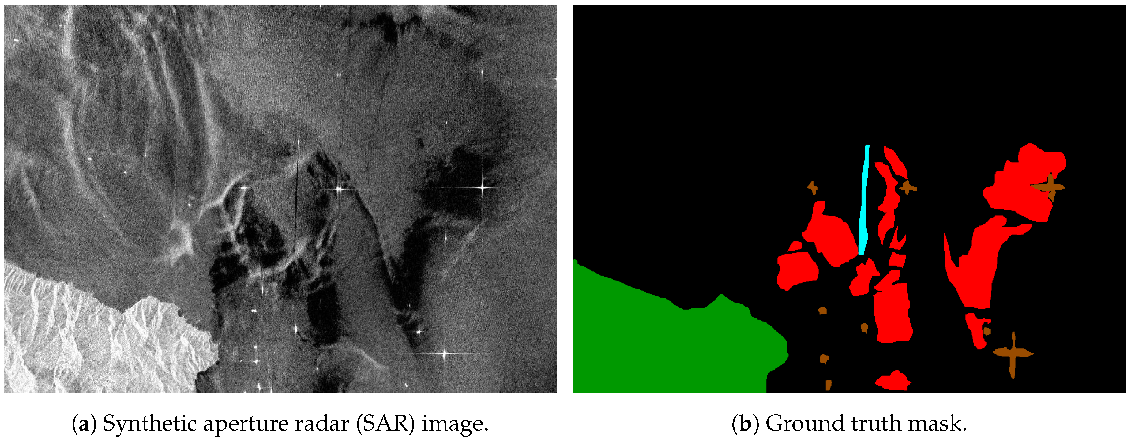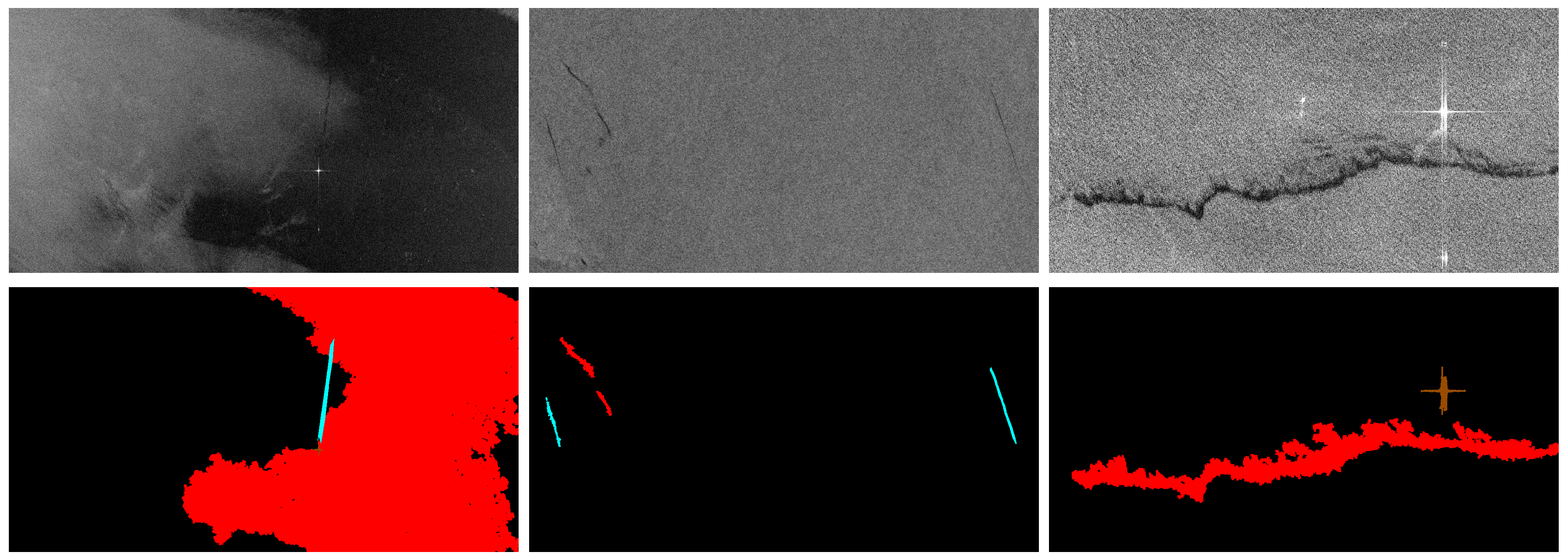The sensor is considered an ideal option due to the all-weather and varying illumination conditions effective operation, as well as its robustness to cloud occlusions [1,3,5]. One of the main aspects of oil spreading over sea surface is that it dampens the capillary waves and so, the backscatter radio waves are suppressed. As a result, oil spills are depicted as black spots, contrary to the brighter regions which are usually related with unspoiled polluted sea areas [2,4]. Moreover, the wide coverage that the sensor can provide is of high significance, since oil spills could cover kilometers, as well as further contextual information, such as close-coastal region or vessels, which can be enclosed in the acquired image. However, similar dark instances could be identified in SAR images that might correspond to potential oil spills. Oceanic natural phenomena such as low wind speed regions, weed beds and algae blooms, wave shadows behind land, grease ice, etc. [3,6,7,8] can also be depicted as dark spots. These dark regions are frequently categorized as look-alikes, rendering the oil spill detection problem even more challenging.

Several classification methods have been proposed to discriminate oil spills from look-alikes over SAR images. In most cases, one specific process is followed, consisting of three main steps: (a) automatic detection of dark spots in the processed SAR image, (b) feature extraction from the initially identified regions, (c) classification as oil slick or regions including look-alikes. During the first step, binary segmentation is usually applied to the input image representation in order to retrieve the depicted black spots. The second phase involves the extraction of statistical features from the aforementioned segmented areas that might include potential oil spills. For the last processing step, either the entire image or sections that contain the black regions of interest are categorized as oil spills or look-alikes. Solberg et al. [9] proposed an automated framework that relies on this three-phase process in order to classify SAR signatures between oil spills and look-alikes. Nonetheless, prior knowledge regarding the probability of oil spill existence must be provided to the classifier. Fiscella et al. [10] proposed a similar probabilistic approach where the processed images are compared in order to define templates and subsequently classify them as oil spill or look-alike. Authors in [11] presented a method to enhance the oil spill recognition system by involving wind history information and provided an estimation about their period of existence. Karantzalos and Argialas proposed in [12] a pre-processing step that improves the classifier’s performance by employing a level-set method for SAR image segmentation in contrast of previous approaches where thresholds or edge detection techniques are applied. Following the most common processing pipeline, a fuzzy logic classifier was presented in [13] to estimate the probability of a dark spot characterized as an oil spill. Although the classification process is automated, an extensive pre-processing phase is required in order to initially extract geographic features. A more object-oriented approach was initially introduced in [14], where a fuzzy classifier was used to label dark spots, while in [15] a decision tree module was used for detected dark spot objects classification. These methods exploited a multi-level segmentation scheme to reduce the false positives rate. Authors in [16] deployed a decision tree forest for efficient feature selection for oil spill classification. Focusing mostly on the detection rather than the recognition of oil spills, Mercier et al. in [17] inserted a semi-supervised detection method using wavelet decomposition on SAR images and a kernel-based abnormal detection scheme.

Considering their robustness in classification objectives, neural networks have also been reported as an efficient alternative in the oil spill detection research area. Neural networks were initially inserted in this research field in [18] where pre-determined features from SAR images were fed to the network in order to estimate relevant labels. In addition, De Souza et al. [19] utilized a neural network for the feature extraction phase towards enriching the internal representations of the input. Similar approaches [20,21] proposed to employ two subsequent neural networks. The first network was deployed to initially segment SAR images and to provide a more effective black spot detection framework while the second was utilized to distinguish oil spills from look-alikes. However, the whole pipeline was not an end-to-end trainable framework since pre-computed features must be provided to the second network for their classification. Authors in [22] employed hand-crafted features to train a wavelet neural network, which classifies black spots captured in SAR images to oil spills and unspoiled water regions. Similarly, Stathakis et al. [23] developed a shallow neural network in order to discriminate oil spills from look-alikes, focused on an optimal solution in terms of computational cost and detection accuracy. Towards this direction, genetic algorithms were used to identify the optimal subset of the extracted features and the optimal number of nodes in the network’s hidden layer. Finally, in [24], a set of image filters and low-level descriptors were used to extract texture information from depicted black spots, which eventually was fed to a neural network, aiming to recognize the spatial patterns of oil spills.

In most cases, a binary classification procedure is involved in the aforementioned methods where either the entire input SAR image or sections are single-labeled as oil spill and/or look-alike. Due to its capabilities in monitoring wide territories, SAR sensor can include further contextual information such as ships, coastal construction, platforms, land, etc. These instances can be semantically meaningful to the classification process, e.g., it is expected that a dark spot with linear formation close to a ship might correspond to an oil spill discharged from the vessel, rather than a look-alike. Moreover, information regarding the presence of nearby coastal territories or ships is important for an early warning system and a decision making module towards mitigating the overall danger. Thus, a different classification approach is required in order to identify properly multi-class instances enclosed in SAR imagery. Furthermore, oil dispersion over sea surfaces is a dynamically evolved phenomenon affected by wind speed, sea currents, etc. Hence, oil slicks present extreme diversity in terms of shape and size. To consider also the physical features of the oil slicks and their dispersion, deep learning techniques can be utilized so that geometrical characteristics like shape, size etc. could be evaluated and efficiently replace the handcrafted features. Taking this into consideration, among with the existence of multi-class instances, semantic segmentation models could be deployed as robust alternatives to extract the rich informative content from SAR images. To this end, Yu et al. [25] introduced adversarial learning of an f-divergence function in order to produce the segmentation mask of a processed SAR image. The authors deployed a deep convolutional neural network (DCNN), denoted as generator, to produce a segmented instance of the input image and a subsequent DCNN, marked as a regressor, to minimize the f-divergence between ground-truth and the generated segmentation result. Nonetheless, the approach is limited to one class (oil spill) segmentation without fully exploiting the pixel-wise classification that semantic segmentation methods can deliver. A convolutional autoencoder network was proposed in [26] to semantically segment scanlines from the Side-Looking Airborne Radar (SLAR) images depicting oil spills and other maritime classes. However, the framework is limited to applying parallel autoencoders for every class, while the robustness of DCNN segmentation models cannot be fully exploited due to the limited number of SLAR data. Authors in [27] presented a DCNN to semantically segment SAR images, yet the process was limited only to oil spill and look-alike identification. 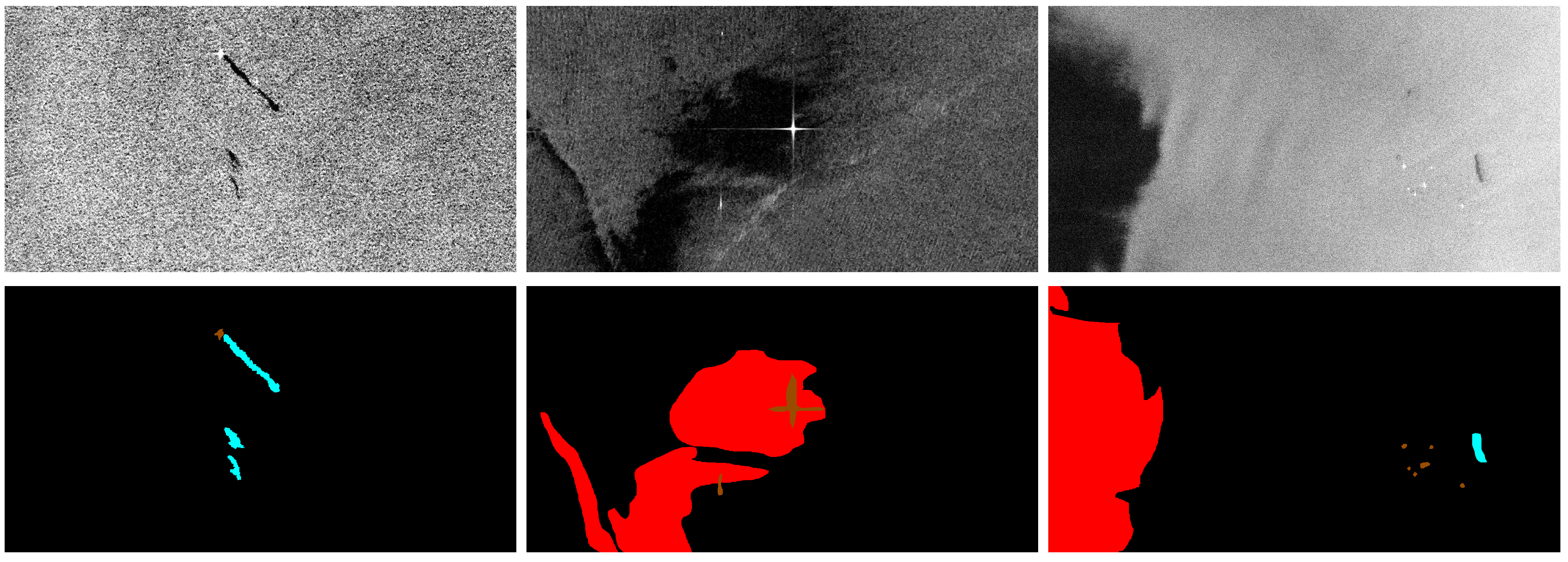An extension of the model was presented in [28] where oil spill, look-alike, land and ship instances were semantically segmented.

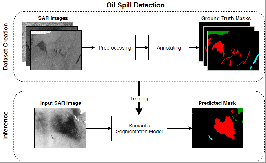
The aforementioned classification-based algorithms relied on abstract datasets for both training and testing and so a proper comparison between relevant approaches is irrelevant due to the lack of a common basis. Moreover, there is no compact formulation to evaluate the efficiency of each algorithm since inputs are manipulated differently following different evaluation techniques according to the corresponding algorithm. To overcome similar issues, we identified the need for a proper public dataset and deliver a common base for evaluating the results of relevant works. Thus, a new publicly available oil spill dataset is presented, aiming to establish a benchmark dataset for the evaluation of future oil spill detection algorithms. Current work relies on the early work of Krestenitis et al. [28] and aims at providing a thorough analysis of multiple semantic segmentation DCNN models deployed for oil spill detection. It should be highlighted that all the tested models were trained and evaluated on the introduced dataset. The main objective is to demonstrate and highlight the significance of DCNN architectures coping the identification problem of oil spills over sea surfaces while the importance of utilizing a common benchmark dataset is also outlined by providing the developed dataset to the relevant research community.

The rest of this paper is organized as follows. In Section 2 the building process of our oil spill dataset is presented and the employed DCNN models for semantic segmentation of SAR images are thoroughly described. The performance of each architecture is presented and compared in Section 3, followed by the relevant discussion. Finally, conclusions are drawn in Section 4.

2. Materials and Methods

2.1. Oil Spill Dataset

The absence of a common dataset for oil spill detection comprises a major limitation that the relevant research community has to address. Previous work [15,16,27] restricted their corresponding activities to customized datasets that were adapted based on the analysis of the approach. However, the presented results are non-comparable since every approach utilizes a different dataset and so, no common base of comparison is established. Considering this deficiency, one of our main objectives was to provide the relevant community a well established dataset properly developed for oil spill identification by processing SAR images. The dataset includes also semantically annotated masks in order for the researchers’ to evaluate their experimental results.

Current subsection includes a thorough analysis and a description of the aforementioned dataset. In brief, satellite SAR images containing oil polluted sea areas were collected via the European Space Agency (ESA) database, the Copernicus Open Access Hub (https://scihub.copernicus.eu/). Information regarding the geographic coordinates and timestamps of the pollution event were provided by the European Maritime Safety Agency (EMSA) through the CleanSeaNet service. Hence, the notation of dark spots depicted in the SAR images as oil spills is confirmed by the EMSA records resulting to a solid ground truth subset. The oil pollution records cover a period from 28 September 2015 up to 31 October 2017 while the SAR images were acquired from the Sentinel-1 European Satellite missions.

Satellites employed for the Sentinel-1 mission are equipped with a SAR system operating at C-band. The ground range coverage of SAR sensor is approximately 250 km with pixel spacing equal to $10\times 10$ m. These specifications indicate the capability of the SAR sensor to cover wide areas of interest and simultaneously the adversity to capture instances of relative small size, e.g., ships. The polarization of the radar image is dual, i.e., vertical polarization transmitted—vertical polarization received (VV) and vertical polarization transmitted—horizontal polarization received (VH). To build the SAR image dataset only the collected raw data from the VV band were processed, following a series of pre-processing steps in order to extract common visualizations. The pre-processing scheme included the following phases:

• Every confirmed oil spill was located according to EMSA records.
• A region containing oil spills and possibly other contextual information of interest was cropped from the raw SAR image. The cropped image was re-scaled to meet the resolution of $1250\times 650$ pixels.
• In order to project every $1250\times 650$ image into the same plane, radiometric calibration was applied.
• A speckle filter was used to suppress the sensor noise scattered in the entire image. Since speckle noise has granular texture, a $7\times 7$ median filter was employed for its suppression.
• A linear transformation was applied for dB to real luminosity values conversion.

Through this process, a set of 1112 images were extracted from the raw SAR data, that consist the main data to be exploited. The images contain instances from 5 classes of interest, namely oil spills, look-alikes, ships, land and sea surface where the latter is always considered as a background class. Every image is annotated combining the information provided by the EMSA records and human identification for maximum efficiency. Since the presented dataset is adapted to be utilized by semantic segmentation approaches, a distinct RGB color was associated to each one of the 5 classes. Hence, every instance of interest is colored according to the identified class, resulting in the ground truth masks that accompany the images of the dataset. The masks are mostly useful for the visualization of the semantic information however, for the training and the evaluation process, $1D$ target labels are required instead of RGB values. Thus, single-channel label masks are also provided by defining an integer value from 0 to 4 for each color class. In Figure 1, an extracted SAR image accompanied with the ground truth mask are presented.

Annotated dataset was split into a training ($90\%$) and a testing ($10\%$) subset, containing 1002 and 110 images, respectively. Due to the nature of oil spill detection problem over SAR images, there is a high imbalance between the instances of the different classes. More specifically, samples of sea surface or land class are expected to dominate across the dataset. On the other hand, oil spills and look-alikes are usually extended in smaller regions of SAR images. However, look-alikes can cover wider areas due to natural phenomena such as low wind speed and wave shadows close to land. Regarding the samples of the “ship” class, these are expected to enumerate significantly less instances since their presence is not guaranteed in an oil pollution scene. On the contrary, when they are depicted, the corresponding instances display a much smaller size compared to the other classes. To address this issue, we focused on creating a well-balanced dataset, by providing a large variety of instances from every class. Thus, our main goal was to have the contextual information of SAR images as equally as possible distributed among the five classes, yet without canceling the challenging and realistic nature of the dataset. To further demonstrate the samples’ imbalance among the classes, due to the nature of the oil spill detection problem, the number of pixels belonging to each class is reported in

Table 1. Number of pixels for each class.

Model	Pixels
Sea Surface	797.7M
Oil Spill	9.1M
Look-alike	50.4M
Ship	0.3M
Land	45.7M

.

As it was highlighted, oil slicks display extreme diversion in shape and size over the sea surface. Moreover, objects depicted in SAR imagery might vary in scale according to the operational altitude of the sensor. Towards developing a meaningful dataset that can be utilized for training purposes of some segmentation models robust to scale variability, we applied a multi-scale scheme for image extraction. Thus, contextual information depicted in SAR raw data is extracted in gradual zoom levels in order to capture instances of interest in various sizes and provide a dataset with high scale diversity. An example of multi-scale scheme for image extraction is presented in Figure 2.

To further illustrate the complexity of the oil spill detection problem, a number of SAR image samples from our dataset, accompanied with the corresponding ground truth mask are presented in Figure 3. These examples can be considered as worst-case scenarios in the detection procedure. It can be observed that the distinction of oil spills and look-alikes comprises a difficult task. Black spots covering large areas of SAR images are usually related to look-alikes contrary to the elongated dark spots of oil spills. However, this is not always the case since proportional SAR signatures can be produced by organic film, wind or sea currents, etc. The contrast of a depicted oil spill compared to the sea surface is crucial as low-level contrasts might lead to vague outlines. Additionally, the detection of an oil spill surrounded by a wider look-alike area consists of a significantly challenging situation since the shape of the oil slick is ambiguous. Considering that the first layers of a DCNN extract low-level features like detected edges, corners, texture, etc, objects with blurry boundaries cannot be identified accurately. On the contrary, a ship instance which was detected near a black spot enhances the probability of an oil spill existence due to an illegal oil discharge. Yet, vessel-generated waves leave similar traces, making the classification of dark spots even lesser accurate. Finally, due to their physical size, ship instances are marginally visible by a SAR sensor in high operational altitudes (upper left image in Figure 3) and when depicted, the corresponding objects cover a very limited area in the acquired image.

On the contrary, oil spill dataset samples provided in Figure 4 denote the simplest cases in comparison with the corresponding events of Figure 3. Captured oil spills are depicted in high contrast to the sea surface posing their boundaries explicitly. Wider look-alike areas can be distinguished accurately from the characteristic oil spill linear traces. Finally, ship instances can be clearly captured from an appropriate operational altitude since they can be efficiently identified by a DCNN segmentation model due to their apparent size.

The developed oil spill dataset aims to assist the research community to exploit a common evaluation base and for this objective, it is publicly available through our lab’s website (https://mklab.iti.gr/results/oil-spill-detection-dataset/). In addition, it is expected that its usage will enhance the research activity of the current field and will lead to robust oil spill detection models, despite its tremendous complexity and diversity. Although it is oriented for semantic segmentation approaches, our dataset can be utilized freely for other methods as well, such as image or object classification by applying minor modifications. Finally, the current version of the dataset can be utilized from researchers that are specialized in feature extraction from SAR images since ground truth masks are provided.

2.2. Semantic Segmentation Models

The following subsection describes all the semantic segmentation models that were deployed as solutions for identifying oil spills over sea surfaces. In general, their majority employs a common encoder-decoder scheme where the network is consisted of two basic components. The first module comprises the encoder block that aims at encoding the input image into a dense and compressed feature vector. Through this process, the spatial dimensions of the feature map are gradually diminishing resulting to a compact representation of the input, which, however, contains high discriminative power. For this step, several pre-trained DCNNs can be used as a backbone of the encoder. Consequently, the extracted representation has to be up-sampled in order to produce a segmented result that meets the dimensions of the original image. For this objective, the decoder block is commonly utilized aiming at progressively reconstructing the encoder’s output. Several techniques have been proposed to increase the spatial dimensions of the encoded vector, usually based on a bilinear interpolation approach and a transposed convolution, i.e., deconvolution. The analysis of this subsection includes the presentation of different semantic segmentation models focusing mostly on the details of the encoder-decoder architecture.

2.2.1. U-Net

The U-Net [29] architecture was initially proposed for segmenting semantically biomedical images however, its application is not limited [30,31]. U-Net can be considered as an extension of a fully convolution network (FCN) [32], consisted mainly of two parts: the contracting (encoder) and the expansive (decoder) path. The name “U”-Net derives from the symmetric architecture between the encoder and the decoder of the network. The contracting path follows an FCN-based architecture and aims at capturing the content of an image. On the contrary, the expansive path enables the precise localization, by upsampling the extracted feature map while decreasing its filters, resulting to a wider but more shallow representation.

More specifically, the contracting path consists of the alternating application of two $3\times 3$ convolutions and a $2\times 2$ max pooling operation with stride 2. Thus, the feature map is progressively down-sampled while increasing the number of feature channels. Correspondingly, the expansive branch increases gradually the spatial resolution by applying in every step an upsampling of the feature map followed be a $2\times 2$ convolution (“up-convolution”) that decreases the feature channels. Moreover, at every step of the decoder, the upsampled feature map is concatenated with high-resolution features from the corresponding step of the encoder to avoid information loss, followed by two consecutive $3\times 3$ convolutions that halve the feature map channel dimension. As the last step, a $1\times 1$ convolution is applied to the output of the decoder in order to map the feature vector of each pixel to the desired number of classes, producing a pixel-wise segmentation mask.

2.2.2. LinkNet

The main objective of the LinkNet [33] architecture is to provide information at every decoding step extracted from the corresponding encoding block. The aim of this procedure is to recover the spatial information more efficiently through the decoder which was diminished during the encoding procedure. Moreover, sharing learnt knowledge from every encoding to decoding layer, allows the decoder to operate with fewer parameters.

The encoder employs ResNet-18 [34] as a backbone that performs strided convolution in order to downsample the input. Initially, a $7\times 7$ convolution filter with a stride of 2 is applied in the original image, followed by a $3\times 3$ max-pooling operation with stride of 2. The rest of the encoder consists of four residual blocks that gradually downscale the extracted feature map. Correspondingly, the decoder is composed of four blocks, each of which consists of three layers, a $1\times 1$ convolution, a $3\times 3$ full-convolution [32] and an additional $1\times 1$ convolutional layer. The convolutional layers are exploited for progressively reducing the number of the filters, while the intermediate transposed convolutional layer (full-convolution) upsamples the spatial dimensions of the feature map with the application of deconvolution filters initialized with bilinear interpolation. The last block of the decoder consists of a $3\times 3$ transposed convolutional layer, followed by a subsequent convolutional layer of a $3\times 3$ kernel. A final $3\times 3$ transposed convolutional layer follows which restores the original spatial dimensions of the input image.

2.2.3. PSPNet

A Pyramid Scene Parsing Network (PSPNet) [35] was proposed to efficiently capture the global context representation of a scene by employing a pyramid pooling module between the encoding and the decoding blocks. First, the input image is forwarded to the encoder, which is based on a ResNet architecture and is enhanced with dilated convolutions for extracting a feature map. The output of the encoder is fed to the pyramid pooling module, consisted of four parallel branches. Each branch initially applies a pooling operation with bin sizes of $1\times 1$, $2\times 2$, $3\times 3$, $6\times 6$, respectively. The outcome of each pooling layer is fed to a convolutional layer with a $1\times 1$ kernel in order to reduce the filter dimension of every feature map to $1/N$ of the original size, where N is the level size of the pyramid scheme. Bilinear interpolation is applied to the low-dimension features maps in order to regain the spatial size of the initial feature map. Finally, the upsampled feature maps provided by the pyramid pooling module are concatenated with the initial feature map extracted from the encoder. The concatenated feature map is usually interpolated and provided to a convolution layer in order to extract the prediction map.

Aiming at an efficient supervision of the learning process, an auxiliary loss is applied at an earlier stage of the network, e.g., in case of a ResNet-101 architecture after the fourth stage of the model. This can be considered as a deeply supervised training strategy allowing us to train very deep architectures. Loss of both functions is back propagated to all preceding layers during training. However, a weighting factor is added to each loss, in order to guarantee that the main branch softmax loss is preponderant on the training process.

2.2.4. DeepLabv2

DeepLab is a well-known model for semantic segmentation, initially inspired from FCN [32]. The first extension of the initial approach [36], named DeepLabv2 [37] exploits atrous or dilated convolution combined with atrous spatial pyramid pooling (ASPP) in order to achieve a scale invariant encoder with large field-of-view filters, without increasing the number of parameters. The output $\mathbf{y}$ of atrous convolution of 1-D input signal $\mathbf{x}$ with a filter $\mathbf{w}$ of length K, is defined as follows:

$$y\left[i\right]=\sum _{k=1}^{K}x[i+r·k]w\left[k\right],$$

(1)

where i notates the i-th element of vector $\mathbf{y}$, r defines the rate parameter considered as the stride with which signal $\mathbf{x}$ is sampled, while for $r=1$ is a special case of (1) corresponding to the regular convolution. Employing atrous convolution enables us to enlarge the filters’ field-of-view in order to capture larger image context without further increasing the number of parameters or computation costs. Moreover atrous convolution allows us to control the resolution of the DCNN network’s responses. The aim of ASPP is to provide multi-scale information to the model. Towards this direction, the extracted feature map is fed into several branches of atrous convolutions with different dilation rates and finally fusing the result of every branch.

As a backbone, the ResNet-101 [34] is employed, where the output of the last convolutional layer is the feature map fed to a 4-branch ASPP, with rates $r=\{6,12,18,24\}$. The output of ASPP is bilinearly upsampled in order to regain the dimensions of the input image. Bilinear upsampling can be considered as a naive decoder however, it is considered sufficient due to the high resolution reserved by atrous convolution. The DeepLab v2 architecture was originally combined with conditional random fields (CRFs) in order to refine the segmentation results. Assuming that ${\mathbf{x}}_i$ is the label assignment of the pixel i, the employed energy function is:

$$E\left(\mathbf{x}\right)=\sum _i{\theta }_i\left(x_i\right)+\sum _{ij}{\theta }_{ij}(x_i,x_j),$$

(2)

where ${\theta }_i\left(x_i\right)$ is the unary potential equal to ${\theta }_i\left(x_i\right)=-logP\left(x_i\right)$ and $P\left(x_i\right)$ notes the predicted label probability of pixel i by the DCNN, while the pairwise potential ${\theta }_{ij}(x_i,x_j)$ is modeled as in [38]. However, CRF is used as a post-processing step to improve the segmentation mask and the detriment of consisting an end-to-end trainable framework. As applied in [27,28], the CRF step was excluded from the processing pipeline since no value is added in terms of accuracy. This selection was further evaluated and investigated in [28].

In order to confront with the high scale and shape variability of oil spill instances, previous approaches [28] employed a multi-scale process of model input. Three parallel branches of the network are utilized to extract score maps from the original image and two downscaled versions, specifically $50\%$ and $75\%$ of the initial dimensions. Predictions from the three branches are fused to evolve a fourth branch by stacking the score maps and applying a max operator at each position. DCNN branches share the same parameters and loss is calculated in respect to the overall output from the four parallel branches. This multi-scale approach is also examined referenced as “DeepLabv2(msc)”. It should be noted that comparison of DeepLabv2(msc) with the rest of the models is not completely straightforward, since the multi-scale scheme can be considered as an extension of the initial model. A more just comparison would include the application of a multi-scale approach to every model however, this it beyond the scope of the current work. Thus, model DeepLabv2(msc) was included in the presented analysis for compatibility reasons to previous works [28].

2.2.5. DeepLabv3+

The latest upgrade of the DeepLab architecture, named DeepLabv3+ [39] extended the previous versions by adding an effective, yet simple, decoder for refining the segmentation results, aiming at producing distinctive object boundaries. The encoder relies on the DeepLabv3 [40] framework, while a modified Aligned Xception [41,42] model was deployed as a backbone properly adapted to semantic segmentation. Currently, DeepLabv3+ model attains state-of-the-art performances on well-known and generic datasets, namely on PASCAL VOC 2012 [43] and Cityscapes [44].

Xception model is extended with more layers aiming at structuring a deeper network. Moreover, every max pooling operation is substituted by depthwise separable convolution with striding. Depthwise separable convolution is proposed as an efficient technique for calculating standard convolutions with less computational cost. To this end, the convolution operation is divided into two steps: (a) depthwise convolution and (b) pointwise convolution. Depthwise convolution is a spatial process over each channel of the input individually. On the contrary, pointwise convolution is simple convolution with kernel size of $1\times 1$ applied to the output of the depthwise convolution, to combine the spatial information over each channel. Atrous convolution is supported in case of depthwise convolution, leading to atrous separable convolution which can further reduce the computational complexity of the model and extract feature maps of arbitrary resolution. The last modification of the Xception model is to have every $3\times 3$ depthwise convolution followed by a batch normalization and a ReLU activation layer. The output of the encoder backbone is forwarded to an augmented version of ASPP. Apart from the four atrous convolution, ASPP consists of an additional branch which is to provide global context information by applying average pooling over the feature map of the encoder backbone. The outputs of ASPP are concatenated and pass through a convolutional layer with $1\times 1$ kernel, leading to the encoder’s final output.

The decoder module has two inputs: the outcome of the encoding main branch, bilinearly upsampled by a factor of 4 and the low-level feature map extracted from the encoder backbone, processed by an additional $1\times 1$ convolutional layer. This convolution is applied in order to balance the importance between the image low-level features of the backbone and the compressed semantic features of the encoder. Both inputs are concatenated in a feature map on which two consecutive $3\times 3$ convolutions are applied to refine the concatenated features. Finally, the output is bilinearly upsampled by a factor of four to restore the initial dimensions of the input image.

2.3. Experimental Setup

The training and the evaluation of each semantic segmentation model presented in Section 2.2 were conducted using the developed and provided to the community dataset. All models were implemented in Keras framework, apart from Deeplabv2 implementation which was built in Tensorflow. During the training phase, for each epoch, data were augmented by randomly resizing half of the images in a scale between $0.5$ and $1.5$ times of the original size. Moreover, random horizontal and/or vertical flip was applied on half of the images. Finally, a fixed size patch was cropped from the image whose position is randomly selected and aims at improving further the generalization ability of each model. According to the network’s architecture, the patch size may vary. However, in order to compare and evaluate the extracted results more efficiently, the patch size was defined to be nearly equal to $320\times 320$ pixels for every deployed model.

In addition, the learning rate of each model was tuned so that the convergence of the training process could be accomplished within a comparable number of epochs for all the models. However, for model DeepLabv2(msc), the training procedure was immensely computationally expensive due to the applied multi-scale scheme and thus, the model was trained for less epochs. Adam [45] optimization algorithm was selected for all the under-evaluation models while the optimization was in respect to the cross-entropy loss function. Assuming that $\mathbf{p}$ is the primary encoded label and $\mathbf{q}$ the predicted class probabilities vector, cross-entropy loss is defined as:

$$H(p,q)=\sum _n{p}_{i}log{q}_i$$

(3)

for every n class of the dataset.

In order to accurately evaluate the performance of each model, we utilized ResNet-101 as a common backbone architecture except for DeepLabv3+ architecture. For the latter, MobileNetV2 [46] was employed as an encoder backbone, instead of the Xception alternative, due to its correlation with much less parameters and thus, lower computational cost.

Table 2. Training details for each model.

Model	Backbone	Learning Rate
UNet	ResNet-101	5$\times {10}^{-5}$
LinkNet	ResNet-101	5$\times {10}^{-5}$
PSPNet	ResNet-101	1$\times {10}^{-4}$
DeepLabv2	ResNet-101	1.5$\times {10}^{-4}$
DeepLabv2(msc)	ResNet-101	1$\times {10}^{-5}$
DeepLabv3+	MobileNetV2	5$\times {10}^{-5}$

presents the training parameters that were applied for every investigated segmentation model.

For all the conducted experiments, a GeForce GTX 1070 Ti was utilized. Batch size was selected to be equal to 12 patches as the maximum value so that the DeepLabv3+ model could fit in the available GPU. Regarding the batch size of the DeepLabv2 model where the multi-scale scheme was employed, it was determined to be equal to 2 patches due to GPU memory limitations. In

Table 3. Patch size, memory requirements and trainable parameters for each model.

Model	Patch Size	MB Allocated	Parameters
UNet	$320\times 320$	10,789	51.5M
LinkNet	$320\times 320$	10,789	47.7M
PSPNet	$336\times 336$	5413	3.8M
DeepLabv2	$321\times 321$	5413	42.8M
DeepLabv2(msc)	$321\times 321$	6437	42.8M
DeepLabv3+	$321\times 321$	6743	2.1M

, the applied patch size among with the memory requirements and the trainable parameters are presented for each method. Since the UNet and the LinkNet prerequisites for memory allocation exceed the available resources, a GeForce RTX 2080 Ti was employed for both models to successfully evaluate their robustness.

3. Results and Discussion

The performance on the developed dataset for each DCNN segmentation model was evaluated in terms of accuracy and processing time. The evaluation results are presented and thoroughly analyzed in this section.

3.1. Accuracy Evaluation

During the evaluation process, no data augmentation was applied and every testing image was processed by the network displaying its original dimensions. The model performance is measured in terms of intersection-over-union (IoU) which is described as:

$$IoU={\displaystyle \frac{prediction\cap groundtruth}{prediction\cup groundtruth}}={\displaystyle \frac{TP}{FP+TP+FN}}$$

(4)

where TP, FP and FN define the number of true positive, false positive and false negative samples, respectively. IoU is measured for every class (in total 5) of the dataset resulting to the mean IoU (mIoU) as the average IoU measured over each class. In terms of mIoU,

Table 4. Comparison of segmentation models in terms of intersection-over-union (%).

Model	Sea Surface	Oil Spill	Look-alike	Ship	Land	mIoU
UNet	93.90	53.79	39.55	44.93	92.68	64.97
LinkNet	94.99	51.53	43.24	40.23	93.97	64.79
PSPNet	92.78	40.10	33.79	24.42	86.90	55.60
DeepLabv2	94.09	25.57	40.3	11.41	74.99	49.27
DeepLabv2(msc)	95.39	49.53	49.28	31.26	88.65	62.83
DeepLabv3+	96.43	53.38	55.40	27.63	92.44	65.06

reports the highest performances achieved for every segmentation model.

Results imply that DeepLabv3+ model displays the highest overall performance, since the highest mIoU, equal to $65.06\%$, was accomplished. Moreover, the model extracts the maximum accuracy for “look-alike” and “sea-surface” class. For the “oil spill” class considered as the class of the highest interest, the achieved accuracy ($53.38\%$) was negligibly lower than the maximum value reported by UNet architecture ($53.79\%$). The lowest performance in terms of mIoU was equal to $49.27\%$ and reported for the DeepLabv2 model. At this point, the impact of the multi-scale analysis scheme on the model’s performance has to be highlighted since the mean accuracy was increased to $62.83\%$. Regarding the UNet and the LinkNet architecture, the extracted results are promising in terms of mean IoU, despite of their naive architecture, considering that atrous convolution or a pyramid pooling module is not applied. However, the information from each encoder level to the corresponding decoder level is highly beneficial for the oil spill semantic segmentation objective. It should also be highlighted that UNet model displays the highest segmentation accuracy also in “ship” samples. However, the model has been fitted to the specific class at the expense of “sea surface” and “look-alike”, considering the relative low accuracy for both classes. Finally, PSPNet architecture presents higher performance in comparison with the DeepLabv2 model, since the outcome of the spatial pyramid pooling module is combined with local features from the encoder backbone. Despite the highest test accuracy of PSPNet in comparison with the LinkNet using the Cityscapes benchmark dataset, this advantage is not valid for the oil spill detection task. Results imply that the more naive decoder’s architecture of PSPNet compared to UNet and LinkNet, leads to lower test accuracy despite the utilization of the pyramid pooling module.

The diversity and the limitations of the semantic segmentation problem can be also confirmed by the results included in Table 4. It can be observed that there is a trade-off between oil spill and look-alike accuracy. More specifically, for the UNet, LinkNet and PSPNet architectures, the models provide a relatively high accuracy for “oil spill” class at the expense of the look-alike segmentation accuracy. The same phenomenon can be noticed for DeepLabv2 architecture nonetheless, the look-alike accuracy was improved at the cost of IoU for oil spill class. Thus, the DeepLabv3+ model and the DeepLabv2 multi-scale approach can be considered as the most efficient models since the performance for oil spill and look-alike segmentation is equally balanced between the two classes. For better understanding the accuracy trade-off between the segmentation classes, mIoU and IoU over each class are calculated every 50 epochs during the training procedure. Results for every architecture are presented in Figure 5 where IoU of each class is plotted in relation to the number of epochs. For presentation and comparison reasons, the range of x axis is fixed from 50 to 600 epochs. The maximum value of epochs range was selected based on the results of the DeepLabv3+ model which has scored the highest accuracy after 600 epochs of training, as presented in Table 4. As analyzed previously, the DeepLabv2(msc) model was excluded from this evaluation setup due to its high computational cost for the training procedure. Thus, the relative analysis in this case is presented for 200 epochs of training.

Observing the corresponding subfigures of Figure 5, it can be observed that oil spill and look-alike classes are somehow compete since pixels categorized as oil spill instances are miss-classified as look-alike and vise versa. This tendency verifies the complexity of the oil spill detection problem that the research community has to face. A similar behaviour can be observed between look-alike and ship classes, especially in case of the UNet, LinkNet and DeepLabv3+ models. This phenomenon can occur due to the expected imbalance of ship samples in respect to the other classes leading to additional inaccurate classification results.

Towards highlighting the difficulties to distinguish efficiently the required instances, the corresponding performance of the training procedure for the DeepLabv3+ model is provided in Figure 6. The model is not overfitted while it converges for most of the classes after 400 epochs, implying that the class instances of the training set cannot be totally separated. Specifically for the oil spill and the look-alike classes, it can be observed that the model cannot be overfitted over these two classes, since a number of oil spill pixels are miss-classified as look-alike and vise versa. Considering that oil spill and look-alike discrimination is a challenging task, the acquired results comprise a sufficient baseline. Thus, a balanced accuracy over these two classes involves a well trained model, opposite to the case of an overfitted model to one class at the expense of low performance to the other. Based on Figure 6, “Ship” class results present the limited identification of ship instances from SAR images with the exploitation of such approaches nonetheless, this deficiency was expected due to the few number of samples for the training process and the small size of the object to be identified.

3.2. Networks Analysis

In this subsection the appropriateness of the oil spill dataset to train the examined DCNNs is discussed. In Figure 7 the mean IoU, measured in training and testing set over a range of epochs, is presented for each model. Similarly to Figure 5, the analysis was performed for 600 epochs since DeepLabv3+ model resulted the highest accuracy for this number of epochs, apart from DeeLabv2(msc), where the maximum value of epochs range was 200. For PSPNet and DeepLab architectures, the primarily convergence of training and testing accuracy, among with the small gap between the two curves, indicate that the models were not under-fitted. Regarding UNet and LinkNet models, the training accuracy has not converged and a bigger gap between the two curves was reported. These results imply that these models have a tendency to overfitting, however, consideering the convergence of testing accuracy around 600 epochs, it follows that the models are not overfitted for this stage of training. Training of UNet and LinkNet can be considered a more challenging task as they comprise models with the most parameters according to Table 3. Nonetheless, the size of the oil spill dataset, combined with the aforementioned data augmentation approach, are adequate for training the presented models.

3.3. Qualitative Results

In Figure 8 and Figure 9 visual results from the evaluated segmentation models are compared. The DeepLabv3+ model presents adequate performance with sufficient segmented image regions, especially for look-alike and oil spills. On the contrary, the DeepLabv2 model displays the lowest performance regarding in oil spill instances identification. Moreover, the model fails to produce fine segmentations and capture the details of land instances. With the enrichment of the multi-scale analysis, the accuracy is significantly improved based on the visual results for DeepLabv2(msc) nonetheless, the model fails in some cases to accurately identify oil spills or look-alikes. PSPNet presents similarly low performance to DeepLabv2, while in addition, false positives of the oil spill class for the PSPNet model are reported. The visual results in combination with the IoU values presented in Table 4 imply that the model can identify oil spills, to some extent, at the cost of look-alike accuracy. Finally, the Unet and the LinkNet architectures appear to be more robust to ship and oil spill identification however, false positives of look-alike class are reported.

3.4. Inference Time Evaluation

In order to completely evaluate the performance of the deployed models, a comparison in terms of execution time and memory requirements for inference was also conducted.

Table 5. Comparison of segmentation models in terms of inference time.

Model	Inference Time (ms)	MB Allocated
UNet	195	4389
LinkNet	171	4389
PSPNet	89	3877
DeepLabv2	344	6689
DeepLabv2(msc)	623	5413
DeepLabv3+	117	4901

presents the average inference time per image, computed over the 110 images of the validation set and accompanied with the memory allocated for each model. Overall, PSPNet among with the DeepLabv3+ model present the best inference performance. More specifically, PSPNet has the fastest inference time, however, at the cost of accuracy as presented in Table 4. LinkNet and UNet models demonstrate higher inference time despite the fact that the GPU memory allocation is at lower levels compared to the DeepLabv3+ model. This is justifiable due to the consecutive upasampling and concatenation operations that LinkNet and UNet employ at the decoding stage. The DeepLabv2 architecture presents the highest memory allocation and displays the slowest performance, especially for the case of a multi-scale approach. In concluding, taking into consideration the trade-off between the inference time and the detection accuracy, the DeepLabv3+ model comprised the optimal solution for the under-investigation problem since it provides the highest performance with relatively high inference speed.

3.5. Comparison of DeepLab Architectures

As all DeepLab approaches rely on similar architectures, a distinct comparison between the DeepLab alternatives is provided for explicit comparison. In the first two rows of

Table 6. Comparison of DeepLab architectures.

Model	Batch Size	Sea Surface	Oil Spill	Look-Alike	Ship	Land	mIoU
DeepLabv2 [28]	16	93.6	21.0	35.80	11.50	72.0	46.8
DeepLabv2	16	94.28	26.63	39.30	10.14	75.36	49.14
DeepLabv2	12	94.09	25.57	40.3	11.41	74.99	49.27
DeepLabv3+	12	96.43	53.38	55.40	27.63	92.44	65.06

the performance of DeepLabv2 as implemented in [28] is compared with the DeepLabv2 implementation of the current work. The two models are differentiated due to the dataset used for their training process. The DeepLabv2 model deployed for the current work was trained on the presented oil spill dataset while the model in [28] was trained by exploiting a subset of 771 images. Concerning the testing set, in both cases, the same dataset was used in order to acquire results for which the required comparison would be feasible. In particular, apart from the accuracy of the “ship” class which slightly deteriorates, IoU of all classes is increased resulting to an improved mIoU from $46.8$ to $49.1$. Hence, results imply that the model can generalize better when trained efficiently with a larger dataset.

For a more consistent comparison, results provided in Table 4 for the DeepLab-based models are presented also in Table 6. The effect of the batch size for the DeepLabv2 model can be observed by comparing the second and the third row of the table. In the case of 12 patches as batch size, the model presents slightly higher mean-IoU due to the minor improvements in “look-alike” and “ship” classes. However, a larger batch size of 16 patches increases the reported accuracy in the rest classes and thus, improves the model’s generalization ability. On the other hand, DeepLabv3+ clearly outperforms the former versions, despite the smaller batch size used in the training process. It should be highlighted that the DeepLabv3+ model improved the testing accuracy of PASCAL VOC 2012 dataset to $89.0\%$ from the initial value of $79.7\%$, which was reported for the DeepLabv2 method. Although this is not valid in all dataset cases, the upgrades in DeepLab architecture were also beneficial for the oil spill segmentation in SAR images.

4. Conclusions

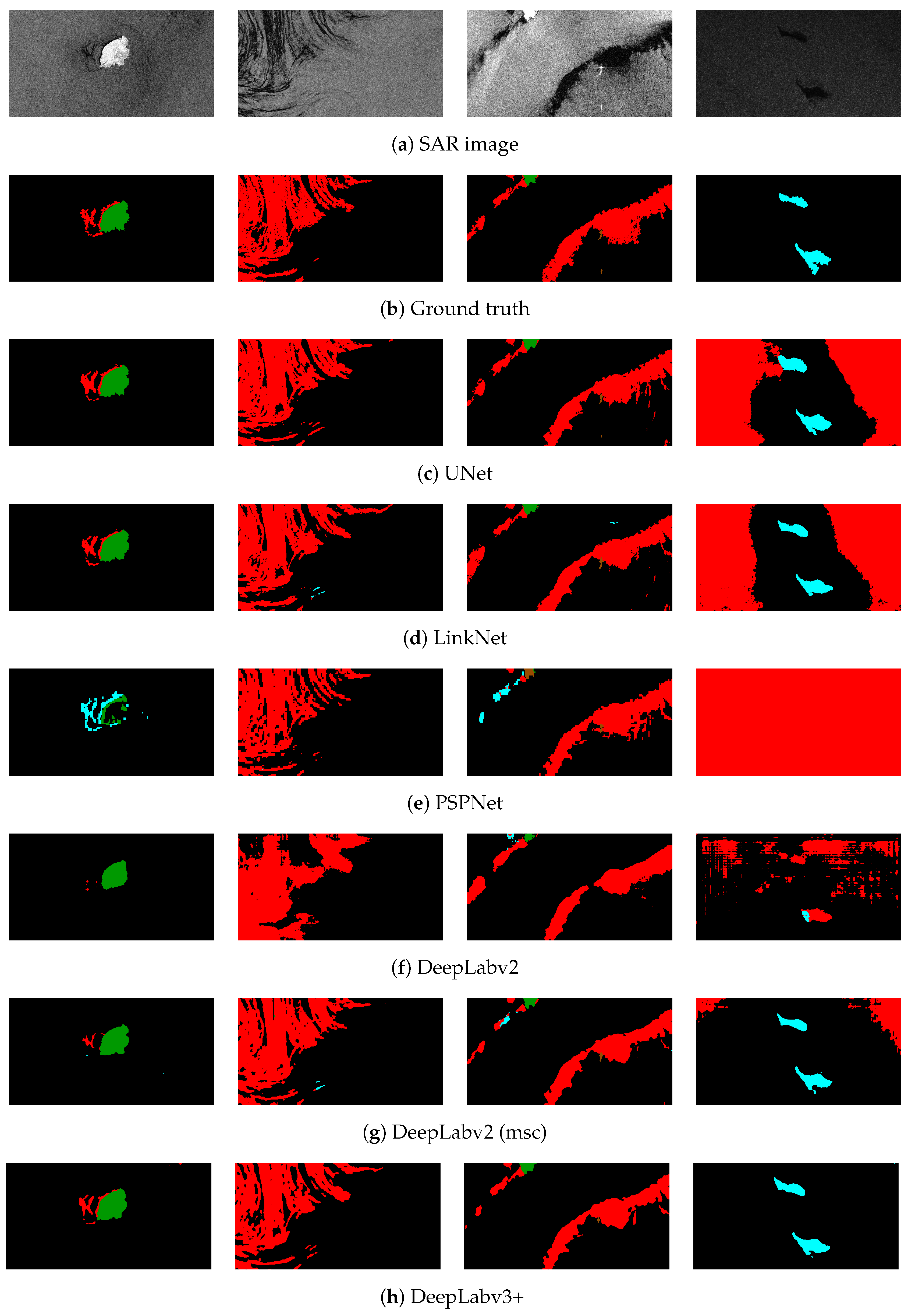
Oil spill comprises one of the major threats for the ocean and the coastal environment, hence, efficient monitoring and early warning is required to confront the danger and limit the environmental damage. Remote sensing via SAR sensors has a crucial role for this objective since they can provide high resolution images where possible oil spills might be captured. Various methods have been proposed in order to automatically process SAR images and distinguish depicted oil spills from look-alikes. As such, semantic segmentation by deploying DCNNs can be successfully applied in the oil spill detection field, since it can provide useful information regarding the depicted pollution scene. In addition, most methods utilize different datasets posing the provided results non-comparable. Based on these two aspects, the main contribution of the paper is twofold: analyze semantic segmentation algorithms and develop a common database consisted of SAR images.

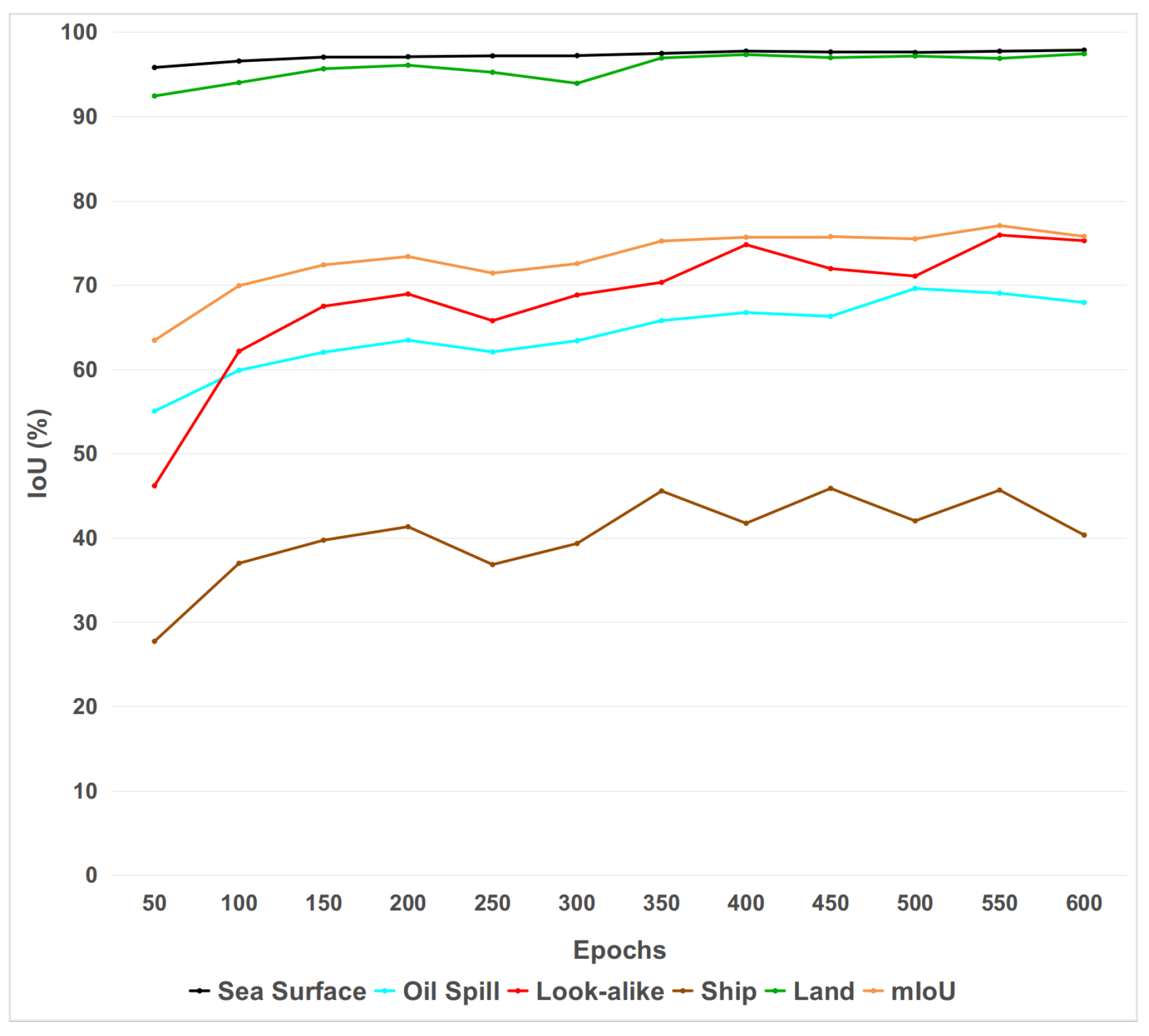
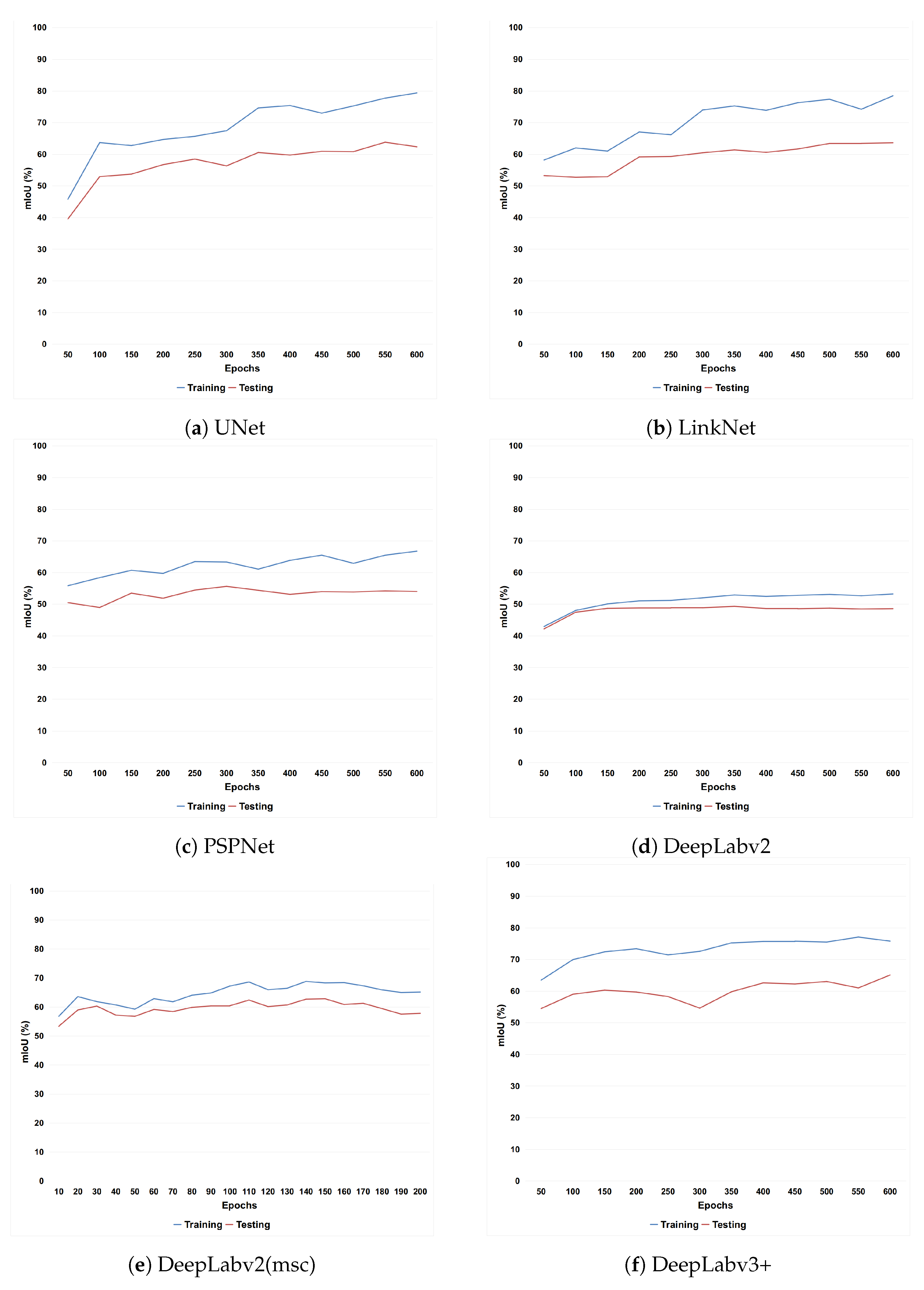
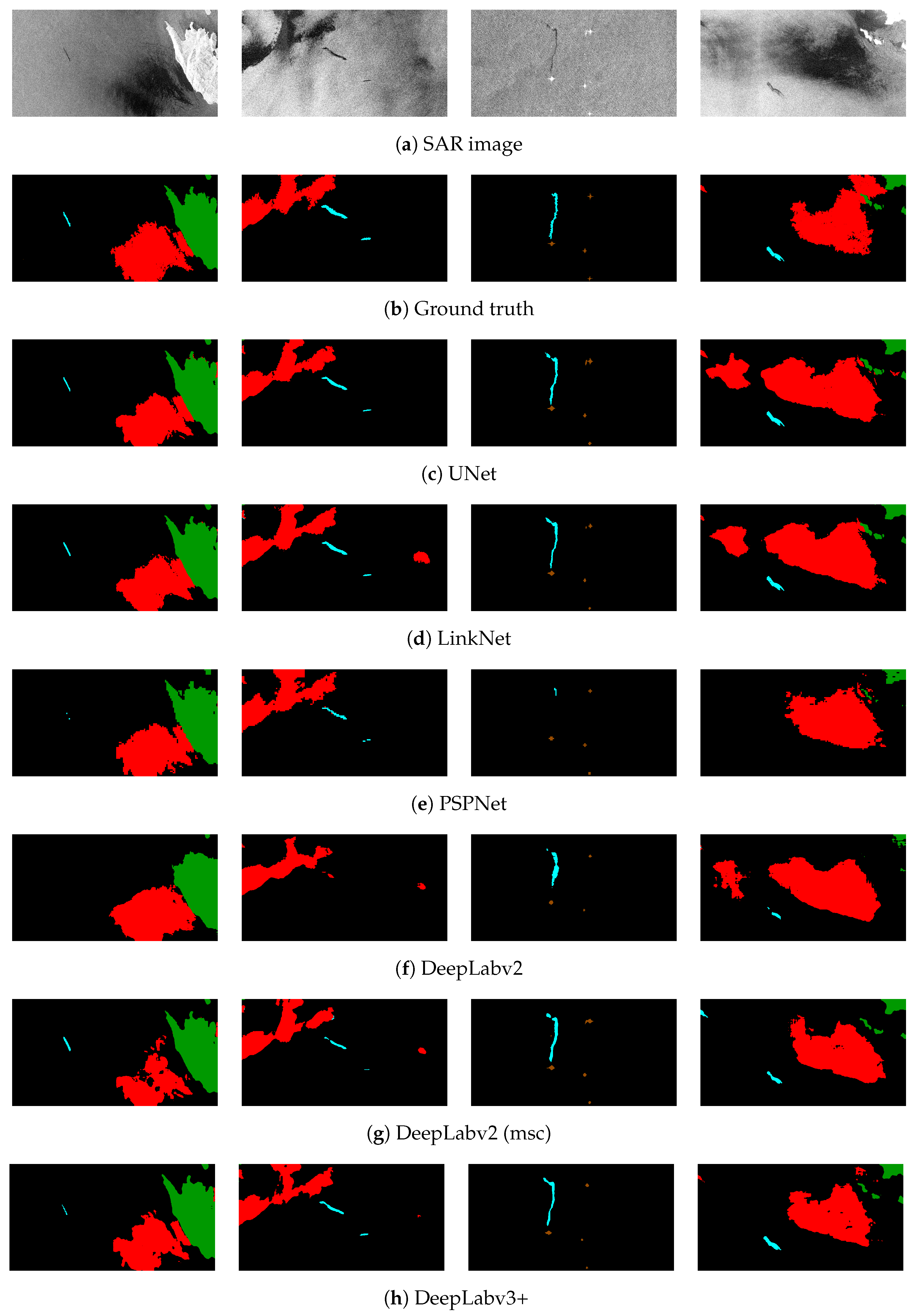
More specifically, extensive experiments were conducted and focused on the use of different DCNN architectures for oil spill detection through semantic segmentation. Every deployed model was trained and evaluated using a common base as a dataset. In general, the DeepLabv3+ model scored the best performance reporting the highest accuracy in terms of IoU and high inference time. The semantic segmentation of SAR images comprises a very challenging task due to the required in situ distinction between the oil spills and look-alikes. The complexity of the posed problem was extensively discussed and accompanied with the relative figures. Finally, a further comparison of different DeepLab architectures was provided confirming the superiority of the DeepLabv3+ model compared to previous approaches. Moreover, the insertion of an annotated dataset consisted of SAR images was provided aiming at being utilized as a benchmark for oil spill detection methods. The presented dataset was developed for training and testing of the segmentation models nonetheless, it can be exploited also in different approaches. Thus, it is expected to contribute significantly towards the efficient application of relevant oil spill detectors.

In the future, accurate models trained on the developed dataset can be encapsulated in a wider framework for oil spill identification and decision making modules. Finally, the semantic segmentation approaches can be extended to other research fields exploiting remote sensing, such as flood or fire detection, precision agriculture, etc. Towards this direction, oil spill dataset can be utilized additionally to train robust backbones of the employed DCNN segmentation models, on a case-by-case basis.

References

1. Brekke, C.; Solberg, A.H. Oil spill detection by satellite remote sensing. Remote Sens. Environ. 2005, 95, 1–13. [Google Scholar] [CrossRef]
2. Topouzelis, K. Oil spill detection by SAR images: Dark formation detection, feature extraction and classification algorithms. Sensors 2008, 8, 6642–6659. [Google Scholar] [CrossRef] [PubMed]
3. Solberg, A.H.S. Remote sensing of ocean oil-spill pollution. Proc. IEEE 2012, 100, 2931–2945. [Google Scholar] [CrossRef]
4. Solberg, A.H.; Brekke, C.; Husoy, P.O. Oil spill detection in Radarsat and Envisat SAR images. IEEE Trans. Geosci. Remote Sens. 2007, 45, 746–755. [Google Scholar] [CrossRef]
5. Fingas, M.; Brown, C. Review of oil spill remote sensing. Mar. Pollut. Bull. 2014, 83, 9–23. [Google Scholar] [CrossRef] [PubMed] [Green Version]
6. Fingas, M.F.; Brown, C.E. Review of oil spill remote sensing. Spill Sci. Technol. Bull. 1997, 4, 199–208. [Google Scholar] [CrossRef] [Green Version]
7. Espedal, H.; Johannessen, O. Cover: Detection of oil spills near offshore installations using synthetic aperture radar (SAR). Int. J. Remote Sens. 2000, 21, 2141–2144. [Google Scholar] [CrossRef]
8. Kapustin, I.A.; Shomina, O.V.; Ermoshkin, A.V.; Bogatov, N.A.; Kupaev, A.V.; Molkov, A.A.; Ermakov, S.A. On Capabilities of Tracking Marine Surface Currents Using Artificial Film Slicks. Remote Sens. 2019, 11, 840. [Google Scholar] [CrossRef]
9. Solberg, A.S.; Storvik, G.; Solberg, R.; Volden, E. Automatic detection of oil spills in ERS SAR images. IEEE Trans. Geosci. Remote Sens. 1999, 37, 1916–1924. [Google Scholar] [CrossRef] [Green Version]
10. Fiscella, B.; Giancaspro, A.; Nirchio, F.; Pavese, P.; Trivero, P. Oil spill detection using marine SAR images. Int. J. Remote Sens. 2000, 21, 3561–3566. [Google Scholar] [CrossRef]
11. Espedal, H. Satellite SAR oil spill detection using wind history information. Int. J. Remote Sens. 1999, 20, 49–65. [Google Scholar] [CrossRef]
12. Karantzalos, K.; Argialas, D. Automatic detection and tracking of oil spills in SAR imagery with level set segmentation. Int. J. Remote Sens. 2008, 29, 6281–6296. [Google Scholar] [CrossRef]
13. Keramitsoglou, I.; Cartalis, C.; Kiranoudis, C.T. Automatic identification of oil spills on satellite images. Environ. Model. Softw. 2006, 21, 640–652. [Google Scholar] [CrossRef]
14. Karathanassi, V.; Topouzelis, K.; Pavlakis, P.; Rokos, D. An object-oriented methodology to detect oil spills. Int. J. Remote Sens. 2006, 27, 5235–5251. [Google Scholar] [CrossRef]
15. Konik, M.; Bradtke, K. Object-oriented approach to oil spill detection using ENVISAT ASAR images. ISPRS J. Photogramm. Remote Sens. 2016, 118, 37–52. [Google Scholar] [CrossRef]
16. Topouzelis, K.; Psyllos, A. Oil spill feature selection and classification using decision tree forest on SAR image data. ISPRS J. Photogramm. Remote Sens. 2012, 68, 135–143. [Google Scholar] [CrossRef]
17. Mercier, G.; Girard-Ardhuin, F. Partially supervised oil-slick detection by SAR imagery using kernel expansion. IEEE Trans. Geosci. Remote Sens. 2006, 44, 2839–2846. [Google Scholar] [CrossRef]
18. Del Frate, F.; Petrocchi, A.; Lichtenegger, J.; Calabresi, G. Neural networks for oil spill detection using ERS-SAR data. IEEE Trans. Geosci. Remote Sens. 2000, 38, 2282–2287. [Google Scholar] [CrossRef] [Green Version]
19. de Souza, D.L.; Neto, A.D.; da Mata, W. Intelligent system for feature extraction of oil slick in sar images: Speckle filter analysis. In Proceedings of the International Conference on Neural Information Processing, Hong Kong, China, 3–6 October 2006; Springer: Berlin/Heidelberg, Germany, 2006; pp. 729–736. [Google Scholar]
20. Topouzelis, K.; Karathanassi, V.; Pavlakis, P.; Rokos, D. Detection and discrimination between oil spills and look-alike phenomena through neural networks. ISPRS J. Photogramm. Remote Sens. 2007, 62, 264–270. [Google Scholar] [CrossRef]
21. Singha, S.; Bellerby, T.J.; Trieschmann, O. Satellite oil spill detection using artificial neural networks. IEEE J. Sel. Top. Appl. Earth Obs. Remote Sens. 2013, 6, 2355–2363. [Google Scholar] [CrossRef]
22. Song, D.; Ding, Y.; Li, X.; Zhang, B.; Xu, M. Ocean oil spill classification with RADARSAT-2 SAR based on an optimized wavelet neural network. Remote Sens. 2017, 9, 799. [Google Scholar] [CrossRef]
23. Stathakis, D.; Topouzelis, K.; Karathanassi, V. Large-scale feature selection using evolved neural networks. In Image and Signal Processing for Remote Sensing XII, Proceedings of the International Society for Optics and Photonics, Stockholm, Sweden, 2006; SPIE: Bellingham, WA USA, 2006; Volume 6365, p. 636513. [Google Scholar]
24. Garcia-Pineda, O.; Zimmer, B.; Howard, M.; Pichel, W.; Li, X.; MacDonald, I.R. Using SAR images to delineate ocean oil slicks with a texture-classifying neural network algorithm (TCNNA). Can. J. Remote Sens. 2009, 35, 411–421. [Google Scholar] [CrossRef]
25. Yu, X.; Zhang, H.; Luo, C.; Qi, H.; Ren, P. Oil spill segmentation via adversarial f-divergence learning. IEEE Trans. Geosci. Remote Sens. 2018, 56, 4973–4988. [Google Scholar] [CrossRef]
26. Gallego, A.J.; Gil, P.; Pertusa, A.; Fisher, R.B. Semantic Segmentation of SLAR Imagery with Convolutional LSTM Selectional AutoEncoders. Remote Sens. 2019, 11, 1402. [Google Scholar] [CrossRef]
27. Orfanidis, G.; Ioannidis, K.; Avgerinakis, K.; Vrochidis, S.; Kompatsiaris, I. A deep neural network for oil spill semantic segmentation in SAR images. In Proceedings of the 2018 25th IEEE International Conference on Image Processing (ICIP), Athens, Greece, 7–10 October 2018; IEEE: Piscataway, NJ, USA, 2018; pp. 3773–3777. [Google Scholar]
28. Krestenitis, M.; Orfanidis, G.; Ioannidis, K.; Avgerinakis, K.; Vrochidis, S.; Kompatsiaris, I. Early Identification of Oil Spills in Satellite Images Using Deep CNNs. In Proceedings of the International Conference on Multimedia Modeling, Thessaloniki, Greece, 8–11 January 2019; Springer: Berlin/Heidelberg, Germany, 2019; pp. 424–435. [Google Scholar]
29. Ronneberger, O.; Fischer, P.; Brox, T. U-net: Convolutional networks for biomedical image segmentation. In International Conference on Medical Image Computing and Computer-Assisted Intervention; Springer: Berlin/Heidelberg, Germany, 2015; pp. 234–241. [Google Scholar]
30. Iglovikov, V.; Shvets, A. Ternausnet: U-net with vgg11 encoder pre-trained on imagenet for image segmentation. arXiv 2018, arXiv:1801.05746. [Google Scholar]
31. Iglovikov, V.; Mushinskiy, S.; Osin, V. Satellite imagery feature detection using deep convolutional neural network: A kaggle competition. arXiv 2017, arXiv:1706.06169. [Google Scholar]
32. Long, J.; Shelhamer, E.; Darrell, T. Fully convolutional networks for semantic segmentation. In Proceedings of the IEEE Conference on Computer Vision and Pattern Recognition, Boston, MA, USA, 7–12 June 2015; pp. 3431–3440. [Google Scholar]
33. Chaurasia, A.; Culurciello, E. Linknet: Exploiting encoder representations for efficient semantic segmentation. In Proceedings of the 2017 IEEE Visual Communications and Image Processing (VCIP), St. Petersburg, FL, USA, 10–13 December 2017; IEEE: Piscataway, NJ, USA, 2017; pp. 1–4. [Google Scholar]
34. He, K.; Zhang, X.; Ren, S.; Sun, J. Deep residual learning for image recognition. In Proceedings of the IEEE Conference on Computer Vision and Pattern Recognition, Las Vegas, NV, USA, 27–30 June 2016; pp. 770–778. [Google Scholar]
35. Zhao, H.; Shi, J.; Qi, X.; Wang, X.; Jia, J. Pyramid scene parsing network. In Proceedings of the IEEE Conference on Computer Vision and Pattern Recognition, Honolulu, HI, USA, 21–26 July 2017; pp. 2881–2890. [Google Scholar]
36. Chen, L.C.; Papandreou, G.; Kokkinos, I.; Murphy, K.; Yuille, A.L. Semantic image segmentation with deep convolutional nets and fully connected crfs. arXiv 2014, arXiv:1412.7062. [Google Scholar]
37. Chen, L.C.; Papandreou, G.; Kokkinos, I.; Murphy, K.; Yuille, A.L. Deeplab: Semantic image segmentation with deep convolutional nets, atrous convolution, and fully connected crfs. IEEE Trans. Pattern Anal. Mach. Intell. 2017, 40, 834–848. [Google Scholar] [CrossRef] [PubMed]
38. Krähenbühl, P.; Koltun, V. Efficient inference in fully connected crfs with gaussian edge potentials. In Advances in Neural Information Processing Systems; Curran Associates, Inc.: New York, NY, USA, 2011; pp. 109–117. [Google Scholar]
39. Chen, L.C.; Zhu, Y.; Papandreou, G.; Schroff, F.; Adam, H. Encoder-decoder with atrous separable convolution for semantic image segmentation. In Proceedings of the European Conference on Computer Vision (ECCV), Munich, Germany, 8–14 September 2018; pp. 801–818. [Google Scholar]
40. Chen, L.C.; Papandreou, G.; Schroff, F.; Adam, H. Rethinking atrous convolution for semantic image segmentation. arXiv 2017, arXiv:1706.05587. [Google Scholar]
41. Chollet, F. Xception: Deep learning with depthwise separable convolutions. In Proceedings of the IEEE Conference on Computer Vision and Pattern Recognition, Honolulu, HI, USA, 21–26 July 2017; pp. 1251–1258. [Google Scholar]
42. Dai, J.; Qi, H.; Xiong, Y.; Li, Y.; Zhang, G.; Hu, H.; Wei, Y. Deformable convolutional networks. In Proceedings of the IEEE International Conference on Computer Vision, Venice, Italy, 22–29 October 2017; pp. 764–773. [Google Scholar]
43. Everingham, M.; Van Gool, L.; Williams, C.K.I.; Winn, J.; Zisserman, A. The PASCAL Visual Object Classes Challenge 2012 (VOC2012) Results. Available online: http://www.pascal-network.org/challenges/VOC/voc2012/workshop/index.html (accessed on 28 March 2019).
44. Cordts, M.; Omran, M.; Ramos, S.; Rehfeld, T.; Enzweiler, M.; Benenson, R.; Franke, U.; Roth, S.; Schiele, B. The cityscapes dataset for semantic urban scene understanding. In Proceedings of the IEEE Conference on Computer Vision and Pattern Recognition, Las Vegas, NV, USA, 27–30 June 2016; pp. 3213–3223. [Google Scholar]
45. Kingma, D.P.; Ba, J. Adam: A method for stochastic optimization. arXiv 2014, arXiv:1412.6980. [Google Scholar]
46. Sandler, M.; Howard, A.; Zhu, M.; Zhmoginov, A.; Chen, L.C. Mobilenetv2: Inverted residuals and linear bottlenecks. In Proceedings of the IEEE Conference on Computer Vision and Pattern Recognition, Salt Lake City, UT, USA, 18–23 June 2018; pp. 4510–4520. [Google Scholar]
Figure 1. (a) Sample of a SAR image and (b) Corresponding annotated image. Cyan color corresponds to oil spills, red to look-alikes, brown to ships, green to land and black is for sea surface.
Remotesensing 11 01762 g001
Figure 2. Extracted images of the same scene for different zoom ratios.
Remotesensing 11 01762 g002
Figure 3. Sample SAR images (left) and corresponding ground truth masks (right) of oil spill dataset considered as worst-case scenarios.
Remotesensing 11 01762 g003
Figure 4. Sample SAR images and corresponding ground truth masks of oil spill dataset considered as plain cases.
Remotesensing 11 01762 g004
Figure 5. Comparison of different architectures in terms of IoU measured in testing set for each class, over a range of training epochs. Black corresponds to “sea surface”, cyan to “oil spill”, red to “look-alike”, brown to “ships” and green to “land” class, while orange is for the reported mean-IoU.
Remotesensing 11 01762 g005
Figure 6. DeepLabv3+: intersection-over-union (IoU) measured on training set for each class in respect to the number of training epochs.
Remotesensing 11 01762 g006
Figure 7. Accuracy in terms of mean-IoU measured in training and testing set for each model, over a range of epochs.
Remotesensing 11 01762 g007
Figure 8. Example 1 of qualitative results of the examined segmentation models on the presented oil spill dataset.
Remotesensing 11 01762 g008
Figure 9. Example 2 of qualitative results of the examined segmentation models on the presented oil spill dataset.
Remotesensing 11 01762 g009