An Integrated Land Cover Mapping Method Suitable for Low-Accuracy Areas in Global Land Cover Maps


1
Key Laboratory of Tibetan Environment Changes and Land Surface Processes, Institute of Tibetan Plateau Research, Chinese Academy of Sciences, Beijing 100101, China
2
CAS Center for Excellence in Tibetan Plateau Earth Sciences, Beijing 100101, China
3
College of Earth and Planetary Sciences, University of Chinese Academy of Sciences, Beijing 100049, China
4
Institute of Remote Sensing and Digital Earth, Chinese Academy of Sciences, Beijing 100101, China
5
Ministry of Education Key Laboratory for Earth System Modeling, Center for Earth System Science, Tsinghua University, Beijing 100084, China
*
Author to whom correspondence should be addressed.
Remote Sens. 2019, 11(15), 1777; https://0-doi-org.brum.beds.ac.uk/10.3390/rs11151777
Submission received: 2 June 2019
/
Revised: 22 July 2019
/
Accepted: 26 July 2019
/
Published: 29 July 2019
(This article belongs to the Special Issue Multi-Modality Data Classification: Algorithms and Applications)
Abstract
:In land cover mapping, an area with complex topography or heterogeneous land covers is usually poorly classified and therefore defined as a low-accuracy area. The low-accuracy areas are important because they restrict the overall accuracy (OA) of global land cover classification (LCC) data generated. In this paper, low-accuracy areas in China (extracted from the MODIS global LCC maps) were taken as examples, identified as the regions having lower accuracy than the average OA of China. An integrated land cover mapping method targeting low-accuracy regions was developed and tested in eight representative low-accuracy regions of China. The method optimized procedures of image choosing and sample selection based on an existent visually-interpreted regional LCC dataset with high accuracies. Five algorithms and 16 groups of classification features were compared to achieve the highest OA. The support vector machine (SVM) achieved the highest mean OA (81.5%) when only spectral bands were classified. Aspect tended to attenuate OA as a classification feature. The optimal classification features for different regions largely depends on the topographic feature of vegetation. The mean OA for eight low-accuracy regions was 84.4% by the proposed method in this study, which exceeded the mean OA of most precedent global land cover datasets. The new method can be applied worldwide to improve land cover mapping of low-accuracy areas in global land cover maps.
1. Introduction
Land cover data are indispensable for many studies and for practical applications such as global change assessment, sustainable development, hydrological modeling and land resource management [1,2,3,4,5,6]. Multiple global land cover datasets have been produced in the last two decades. Most of these datasets were assessed with accuracies of less than 80% by users or producers [7,8,9,10,11,12]. An important reason is that some areas always have relatively low accuracy.
According to an accuracy assessment for global land cover datasets based on 38,664 test samples, some regions located in highly heterogeneous areas have lower accuracies than others [13]. Areas with complex topography or varied land cover types tend to be characterized by high heterogeneity and low accuracy, so they can be included among the low-accuracy areas. In China, the agro-pastoral zone that is located in the semi-humid and semi-arid area of China, for example, is rich in land cover types and the topography of the southern hilly area is complex. Ran et al. and Zeng et al. have shown that the accuracies for these two areas are less than the average accuracy of the whole of China [14,15]. How to improve the accuracy of low-accuracy areas is essential for improving the overall accuracy of land cover mapping at large scale.
Land cover classification (LCC) is a comprehensive process. Every step in the classification process will affect the LCC accuracy including selection of image, training samples, classification algorithm and classification features. In terms of availability and data characteristics, Landsat and Sentinel-2 Imagery are more suitable for LCC of low-accuracy areas because of their fine spatial resolution and free availability [16,17,18]. Landsat is the only sensor that can go back to a historical period [19,20,21]. Sentinel-2 has higher spatial resolution as well as a higher revisit cycle after 2015 [22]. The accuracy of the Moderate Resolution Imaging Spectroradiometer Land Cover Type (MODIS LCT) product has been low. The limiting factor has been mixed land-cover type pixels that were caused by its coarse spatial resolution [15]. However, remote sensing data with high spatial resolution are usually very expensive and are more suitable for studies of small regions.
The classification algorithm is one of the most often studied factors in improving classification accuracy. Classification algorithms perform differently under the different conditions found in different regions. Some popular algorithms like support vector machine (SVM) and random forest (RF) have performed better than many other algorithms [9,23,24,25]. Logistic regression (LR) and logistic model tree (LMT) also produced good results in a comparison with 15 algorithms used to classify regions in southern China [26]. In the past, several different fusion methods have been developed that could combine a number of land-cover classifications. These methods produced a hybrid land-cover map which could not be achieved by any of the individual sources on their own [27,28,29]. The fusion methods are helpful when some of the individual classification data are of relatively better results. In low-accuracy areas where almost all the individual classification data are apt to be of weak performances, fusion of different LCC data is not enough to improve classification accuracy.
Spatial variability is an inherent trait of any terrestrial element, including land cover. The manifestation of spatial variability is that the same land cover type shows different spectral characteristics and topographical features in different regions because of differences of climate, human activity and physical conditions [30]. The high heterogeneity is one of the most important factors that are responsible for the low classification accuracy of low-accuracy area. However, most existing global land cover datasets could not gather large amounts of representative training samples due to lack of sufficient understanding on low-accuracy regions. [7,8,9,10,11,12]. The selection of training samples and features in different regions of low-accuracy areas can correctly identify phenomena such as the same object with different spectra (SODS) and different objects with the same spectrum (DOSS).
The existence of low-accuracy areas is one of the most important limitations in improving global land cover mapping. Few researches have focused on the low-accuracy area and the classification method that aims at this area has not been discussed technically as well. The primary objective of this study is therefore to design an LCC method to improve the land cover mapping accuracy of low-accuracy areas. The method developed in this study is an integrated LCC method as it optimizes the whole classification process including image choosing, training sample selection as well as classification algorithm and features. It improves the images choosing and sample selection based on an existent visually-interpreted LCC dataset. Five algorithms and 16 groups of classification features were compared to decide the optimal classification algorithm and features regionally. The Landsat OLI imagery is the image data source.
Section 2 describes the low-accuracy areas of China, the study sites and datasets that were the focus of this study. Section 3 explains the method. Section 4 provides a detailed description of the results, including the optimal algorithm, the impacts of classification features on accuracy, optimal classification on a region-by-region basis and comparisons of the classifications with existing datasets. Section 5 includes discussions and conclusions. Our goal is to prove that the proposed method is valid in improving classifications of low-accuracy areas.
2. Study Sites and Datasets
2.1. Low-Accuracy Area and Study Sites
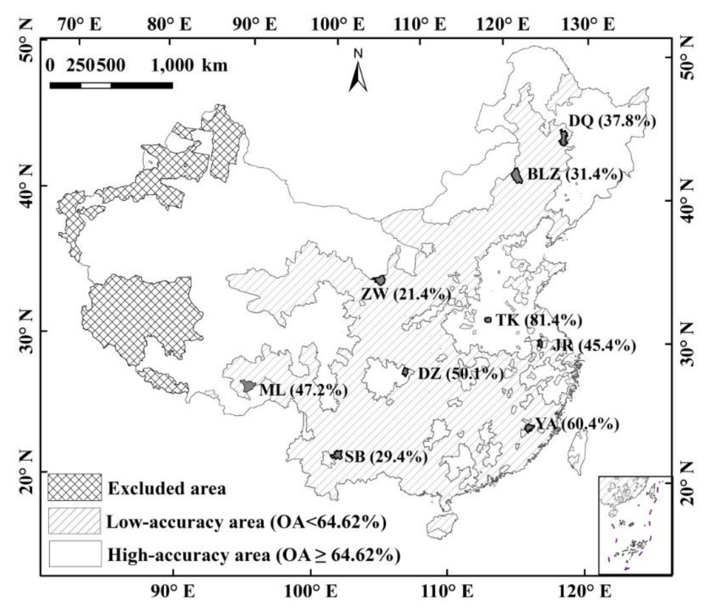
China was chosen as our study area to test the integrated method. Low-accuracy areas of China were defined by the accuracy assessment of MODIS LCT data. We choose MODIS LCT data as the classification data to calculate accuracy because mix pixels that are caused by spatial heterogeneity are the main error sources of MODIS LCT product [15]. Reference data used for accuracy assessment were the 1:10,000 National Land Use Data of China (NLUD-C) [30]. NLUD-C is a dataset totally acquired by visual interpretation of professors in land cover classification. The validation of NLUD-C has been completed by field investigations and the OA of NLUD-C is 96.67%. Because the OA of MODIS LCT over the whole of China is 64.62%, counties with overall accuracies <64.62% were assigned to the low-accuracy category (Figure 1). The low-accuracy areas of China are mainly located in the second-grade area where the terrain is complex and land cover types are various. The low accuracy areas in western parts of Xinjiang province and Tibetan province were excluded from the study (Figure 1) where the difference between MODIS LCT and NLUD-C is mainly caused by seasonal changes of grasslands [15]. The areal proportion of the low-accuracy area in China is 41% without the excluded area.
Nine counties were chosen as study sites for the land cover mapping of low-accuracy areas as follows: Ba Lin Zuo (BLZ), Da Qing (DQ), Da Zhu (DZ), Ju Rong (JR), Mi Lin (ML), Shuang Bai (SB), Tai Kang (TK), Yong An (YA) and Zhong Wei (ZW) (Figure 1). Of these nine counties, one (TK) was located in a plain, high-accuracy area and was used as a control to enable more comprehensive comparisons between algorithms. The other eight counties were located in low-accuracy areas, which were defined as counties with OAs less than the OA for the whole of China (Figure 1). All the study sites were located in different ecological regions of mainland China (Table 1) and three were in agro-pastoral zones (BLZ, DQ and ZW), four were in southern mountainous or hilly regions (DZ, ML, SB and YA) and two were in agricultural areas (TK and JR).
2.2. Datasets
Table 2 lists the datasets used in this study. The data used for classification included Landsat 8 operational land imager (OLI) image data (from Band 1 to Band 7) and topographical data (digital elevation model [DEM], slope and orientation of slope [aspect]). Nine OLI images for the nine study sites used for classification were selected from images that were acquired in 2013 and 2014. The DEM data came from the ASTER Global Digital Elevation Map version 2 (GDEM v2). The slope and aspect data were derived from the DEM data.
The 2013 MODIS 250-m, 16-day enhanced vegetation index (EVI) data (MOD13Q1) were used to decide the time (i.e., day) associated with the images that were finally used in classifications (Table 1). The method is presented in Section 2.2 (Figure S1).
Two existing land-cover datasets were compared with our data to verify the advantage of the provided method. The two datasets are FROM-GLC (Finer Resolution Observation and Monitoring-Global Land cover) and MODIS LCT (MCD12Q1). FROM-GLC is a global land cover dataset produced using Landsat images acquired around 2010 [9] and version 2017 was available for this study. Its self-evaluated accuracy is 64.9%. MCD12Q1 is an annually updated global land cover dataset [8] and version 6.0 was available for this study.
3. Method
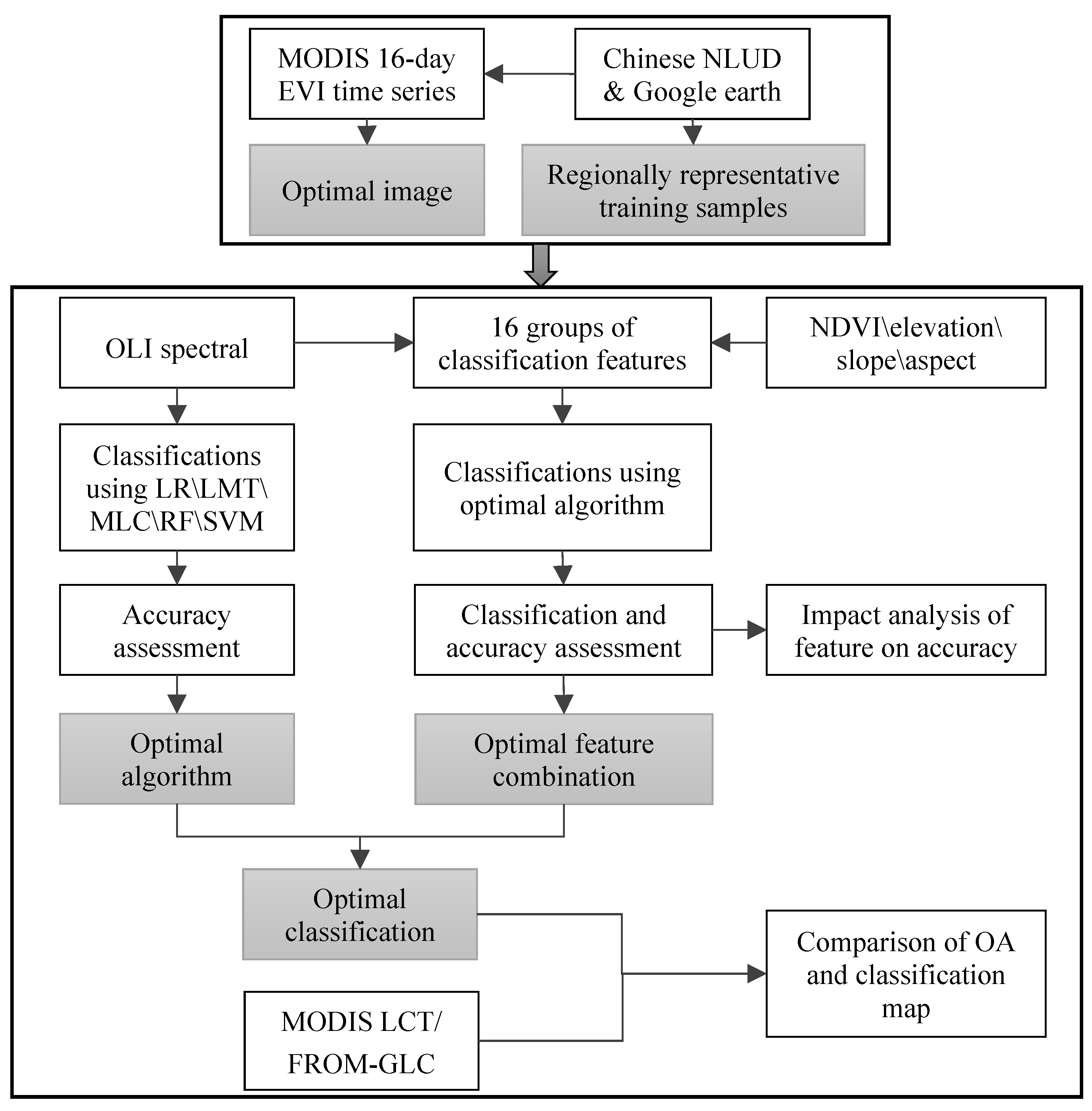
The integrated land cover mapping method is improving the accuracy by optimizing four procedures including choosing images that could better separating vegetation types, selecting training samples with representativeness, as well as producing the optimal classification by using the suitable algorithm and features on a regional basis (Figure 2). The optimization processes of the four procedures are elaborated below.
3.1. Image Selection
Image selection is essential to find the image that can best discriminate between different land cover types, especially vegetation types. The image selection method that we used was based on vegetation phenology and image quality [31] and was carried out in two steps.
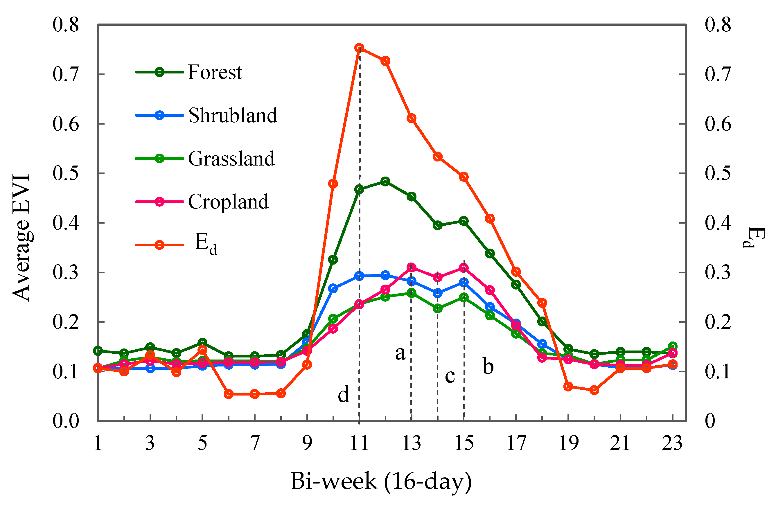
First, an optimal timeframe was determined based on time-series of 16-day EVI and Ed (EVI difference, see Equation (1) of the major land cover types (Figure 3). Time-series of 16-day EVI came from the 2013 MOD13Q1. The Ed quantifies the difference of EVI among all major land cover types. The EVI and Ed for each land cover type were derived by averaging the EVI data for all pixels of that land cover type derived from existing land-cover data (NLUD-C) [30]. The optimal timeframe included two-week periods with peak EVI values of major land cover types or the maximum Ed value. Images in the optimal timeframe facilitated distinguishing between different vegetation types.
where Ei and Ej. are the EVI values of land cover types i and j, respectively, and n is the number of major land cover types.
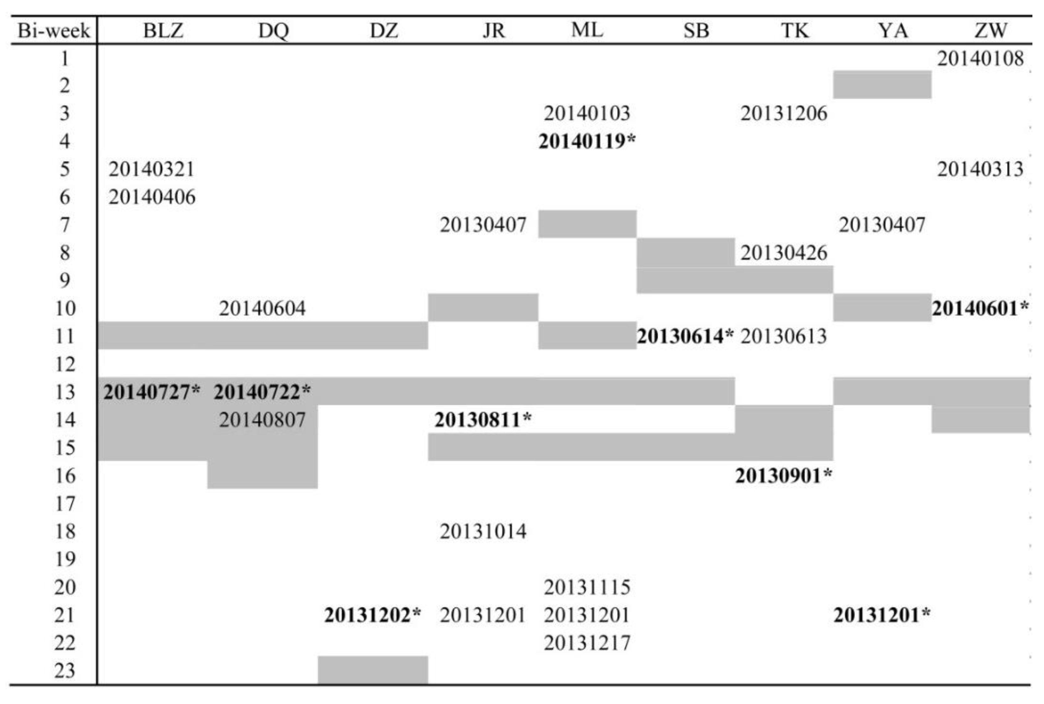
The second step is to pick out the optimal image from the images in 2013 and 2014. Images with cloud cover higher than 30% were removed. Next, the one within the optimal timeframe was picked as the optimal image. When more than two images were available in the optimal timeframe, the one with the larger Ed was chosen. If there was no available image in the optimal timeframe, then the image at the nearest time was selected. Figure A1 presents the results of the selection process.
3.2. Land-Cover Classification System
The land cover classification system used in this study was composed of 10 basic land cover types (Table 3) and was consistent with the classification system used in the FROM-GLC [9]. The classes in the classification system served as the basis for subtly thematic classification, such as a second-level LCC. The conversion from the International Geosphere–Biosphere Program classification system applied to the MODIS LCT dataset to our classification system was completed by aggregating classes at the second level into classes at the first level, as presented by Zeng et al. [15].
3.3. Training and Testing
Training samples were obtained by a sorted selection process. A sub-region for each land-cover type was extracted from the existing land-cover data (NLUD-C) and the same amount of samples was randomly selected for each type. The suggested number of training pixels for each class was required to be 10–30 times the number of feature bands [32,33]. Two hundred fifty pixels were chosen as training samples for each land-cover type in each study site. To verify the classification results, a total of 500 pixels were initially selected randomly as test samples in each study site. Because of this random selection, dominant cover types occupied a majority of the initial samples, whereas some minority or fragmented cover types occupied a small proportion. To circumvent this problem, additional pixels were selected to ensure that at least 30 samples were selected for each of the minority types. The total number of testing pixels for each study region was therefore larger than 500. Training and testing samples were compared and adjusted to avoid using the same sample class as training and testing samples. The numbers of samples are listed in Table 4. The attributes of both training and testing samples were decided by experts who had produced NLUD-C and the attributes were affirmed by using high-resolution images on Google Earth. The interpretation marks were listed in Figure A2 (Figure S2).
3.4. Classification Algorithms and Features
Five algorithms were used in the classification to choose the optimal algorithm, including SVM (Support Vector Machine), LR (Logistic Regression), LMT (Logistic Model Tree), RF (Random Forest) and MLC (Maximum Likelihood Classification). Most of them are chosen because of good performance and popularity. Among the five classification algorithms used for comparison, the MLC, a parametric algorithm, is the most often used statistics-based algorithm and is often taken as a standard for comparison [24,25,34]. Details about the explanation and use of the five algorithms have been explained previously [35,36,37,38,39]. Table 5 lists the values of the parameters for different algorithms. The parameters with multiple values are listed in Table 5 and the parameters need to be adjusted during use to get the best performance in an algorithm. The prior probability value for MLC was set to the same value for all land cover types. Classification features used in the comparison included spectral bands of OLI images (from Band 1 to Band 7), NDVI (Normalized Difference Vegetation Index), elevation, aspect and slope.
3.5. Comparison Analysis
In the comparison, the confusion matrix and OA were the main evaluation indexes. When the algorithms were compared, the first seven bands of OLI images were classification inputs and the algorithm with the highest OA was chosen as the optimal algorithm. Spectral bands plus a single non-spectral band feature (NDVI, elevation, slope or aspect) were classified using the optimal algorithm and the result was compared with the results from only spectral bands as input to assess the impact of non-spectral band features on accuracy. The OAs for the 16 groups of classification features were then compared to determine the optimal combination of classification features on a region-by-region basis. The classification from the optimal algorithm and classification features is the classification result of the integrated land cover mapping method in the study. Finally, our classification data and the FROM-GLC and MODIS LCT data were evaluated with the same testing samples. The overall accuracy and classification results were presented.
4. Results
4.1. Optimal Algorithm
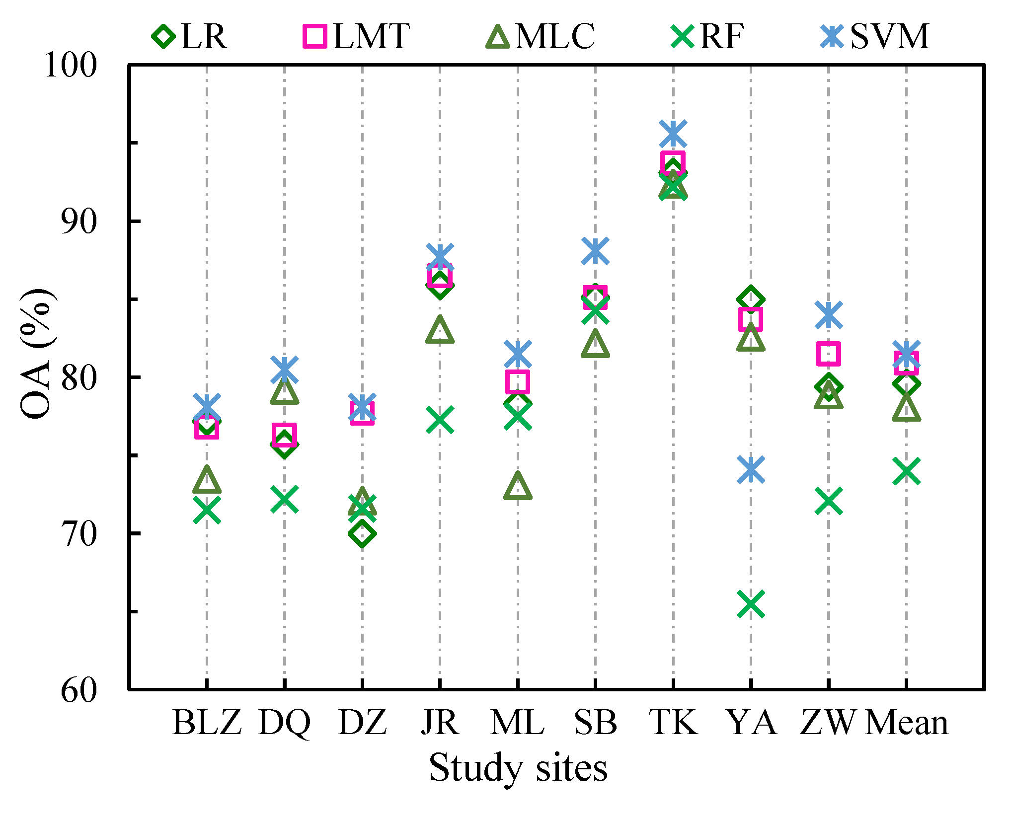
Comparative analysis of overall accuracies identified the SVM as the best algorithm for most study sites when the classification inputs were the spectral bands of OLI images (Figure 4). The accuracy comparison identified LR as the optimal algorithm for YA County. The mean accuracy of study sites in the low-accuracy areas was also the highest for SVM (81.5%) among the five algorithms. The lowest mean accuracies for low-accuracy areas were achieved by RF. The difference between the highest and lowest mean accuracies was 7.5%. The best and worst accuracies achieved in TK County, the high-accuracy region, were also obtained by SVM and RF, respectively and the difference between the high and low accuracy was 3.4%. The superiority of SVM over the other algorithms was therefore more obvious in low-accuracy areas.
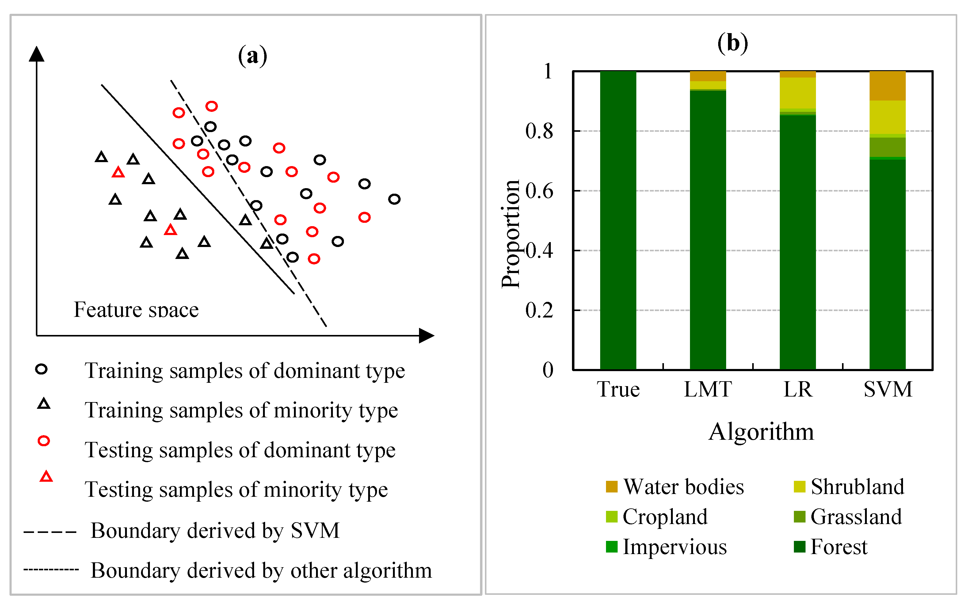
The superiority of the SVM over the other algorithms could be attributed to the fact that it gave more weight to the training samples that lay at the edge of the class distributions in feature space [40]. This advantage was especially valuable when training samples were hard to obtain. It was likely to lead to over-fitting, however, when the area accounted for by the dominant class greatly exceeded the area accounted for by the minority classes and the number of training samples for the different classes was the same. The reason is that the representativeness of training samples among minority class pixels is better than the representativeness of training samples among dominant class pixels (Figure 5a).
The exception that SVM performed worse than other algorithms in YA County could be attributed to over-fitting by SVM. The land-cover types (minority class) other than forest (dominant class) occupied a small proportion of study sites but the fact that the training samples for all cover types included 250 pixels increased the probability of edge pixels for the minority class in training samples. The boundary determined by edge pixels could therefore be trained to include dominant type pixels into minority-type pixels more easily. Many dominant types (forest) pixels were classified incorrectly as minority types (grassland, shrubland and bodies of water) pixels (Figure 5b).
4.2. Impact of Class Features on Accuracy
In addition to classification algorithms, input data are among the factors that can be controlled by analysts to improve accuracy. We chose four classification features as added input data to determine the impact of the added single feature on accuracy, including NDVI, elevation, aspect and slope. The SVM was used in feature-added classifications of eight of the nine sites. LR was used in YA County where LR was the optimal algorithm in the algorithm comparison (Figure 5).
A comparison of the OA with spectral bands as classification input versus spectral bands augmented with NDVI as input (Figure 6) revealed that NDVI caused small differences in accuracy. The slightly positive effect of NDVI can be explained by the fact that NDVI is derived from spectral bands and part of its information has been included in the spectral bands. However, the utility of NDVI in classification is unequivocal, because the impact of NDVI on accuracy is positive under most conditions.
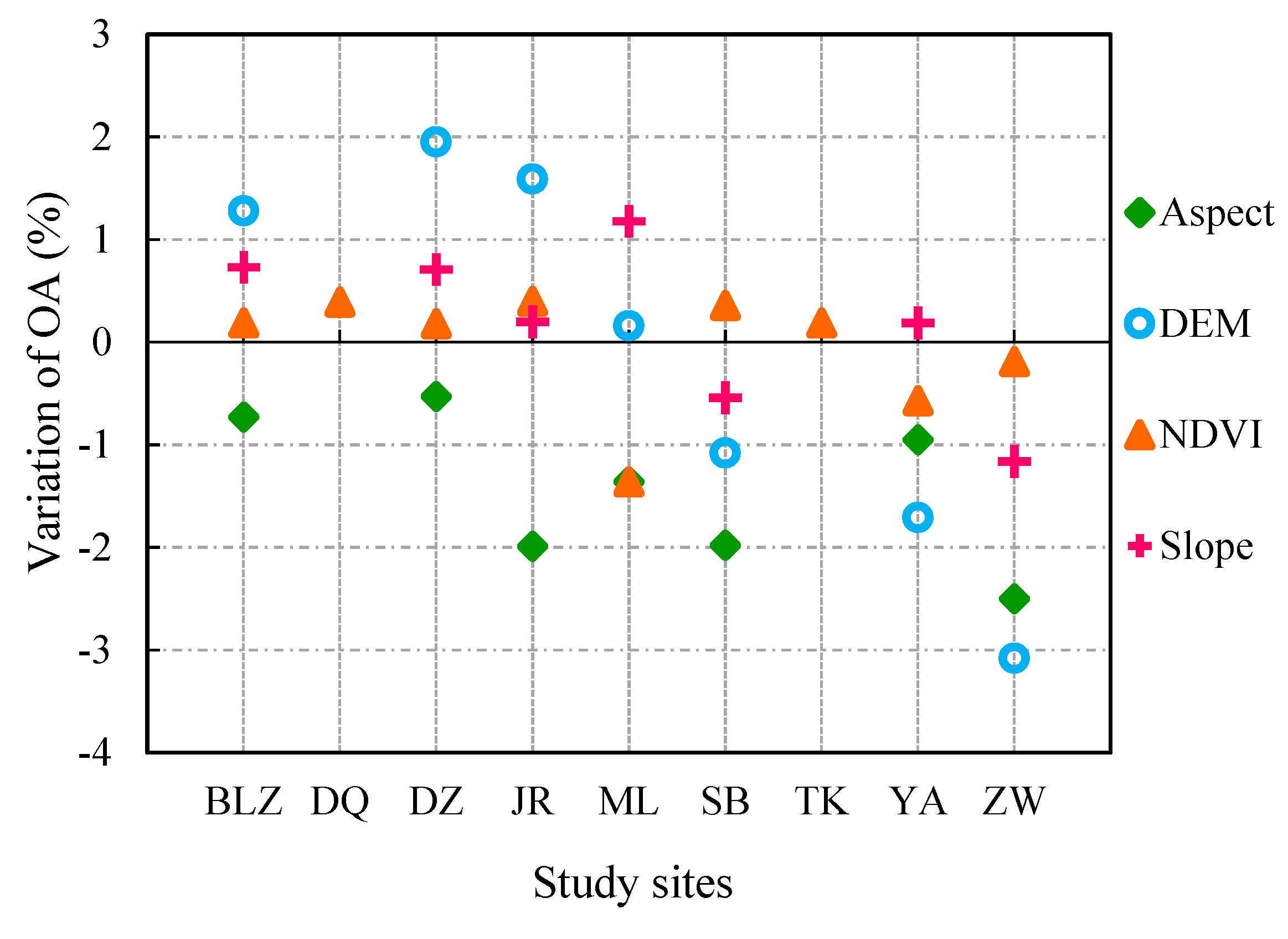
In the case of topographical information, we assessed the impact on OA induced by every terrain feature (elevation, slope and aspect). Figure 6 shows the results of that analysis. We discovered that aspect decreased accuracy at all study sites, whereas the impacts of elevation on accuracy were opposite in mountainous areas and in areas that were combinations of hilly and flat regions, which is the same with slope. These differences were related to the distribution and types of cropland. The amplitudes of the variations were larger when they were induced by elevation than by slope.
The negative effect of aspect reflected the fact that there was an overlap in the distributions of the aspect values of different land cover types. The elevation effect was usually positive in areas where plain regions and hilly regions were both present (such as BLZ, DZ and JR) because either trees or shrubs may grow in hilly regions but croplands are located in plain regions. The negative effects of elevation and slope were caused by the distribution of terraced fields (i.e., cropland) on hills in regions like the Southeast Hilly Area (YA) and Yunnan and Guizhou Plateau (SB). The fact that elevation had a greater effect on accuracy than slope was due to the fact that natural vegetation is affected more by elevation than by slope.
4.3. Optimal Combination of Class Features and Classification Results
To determine the optimal combination of class features for each region, 16 groups of class features were classified using SVM. Table 6 lists the OAs. The combination of class features corresponding to the highest accuracy still indicated that NDVI was necessary and aspect was not needed in most regions. This conclusion affirms the results of the impact analysis of single features.
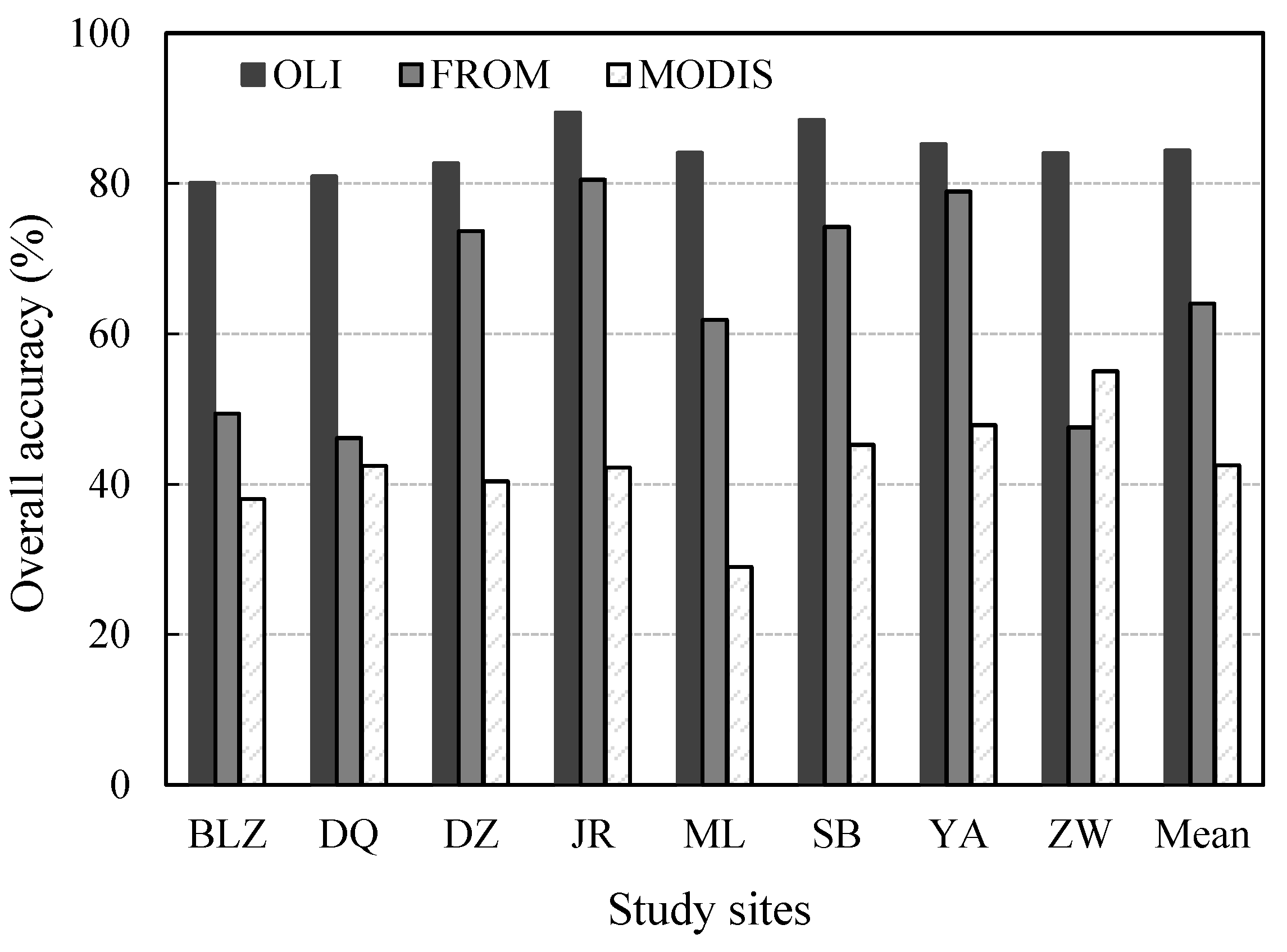
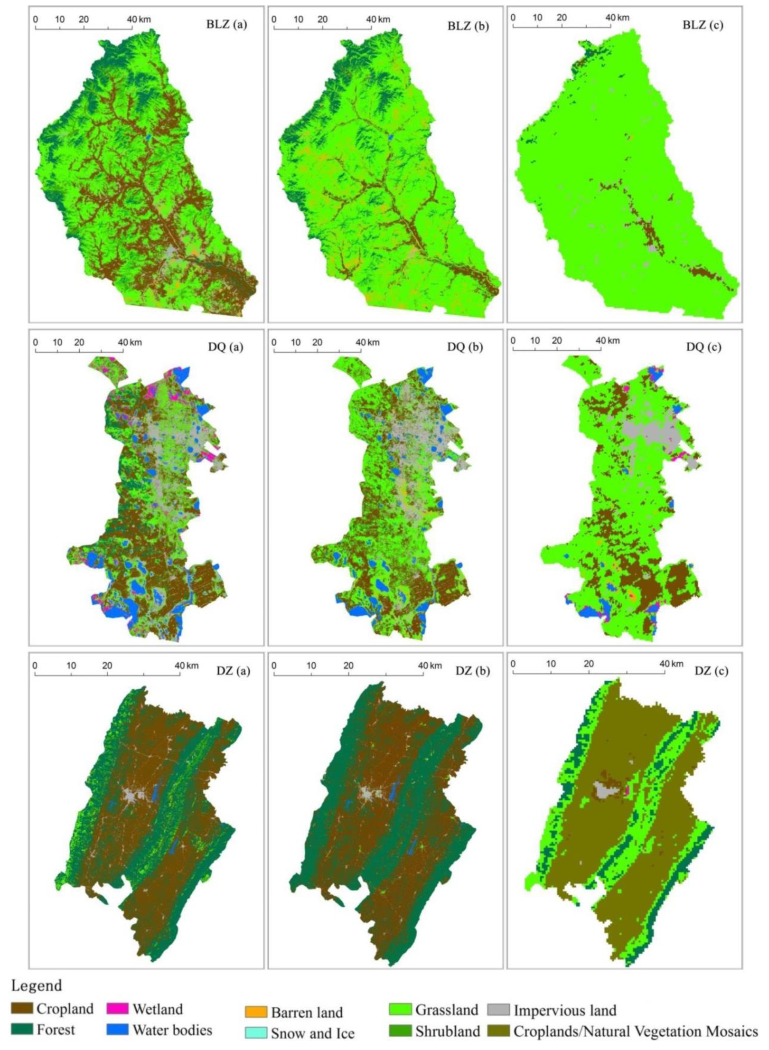
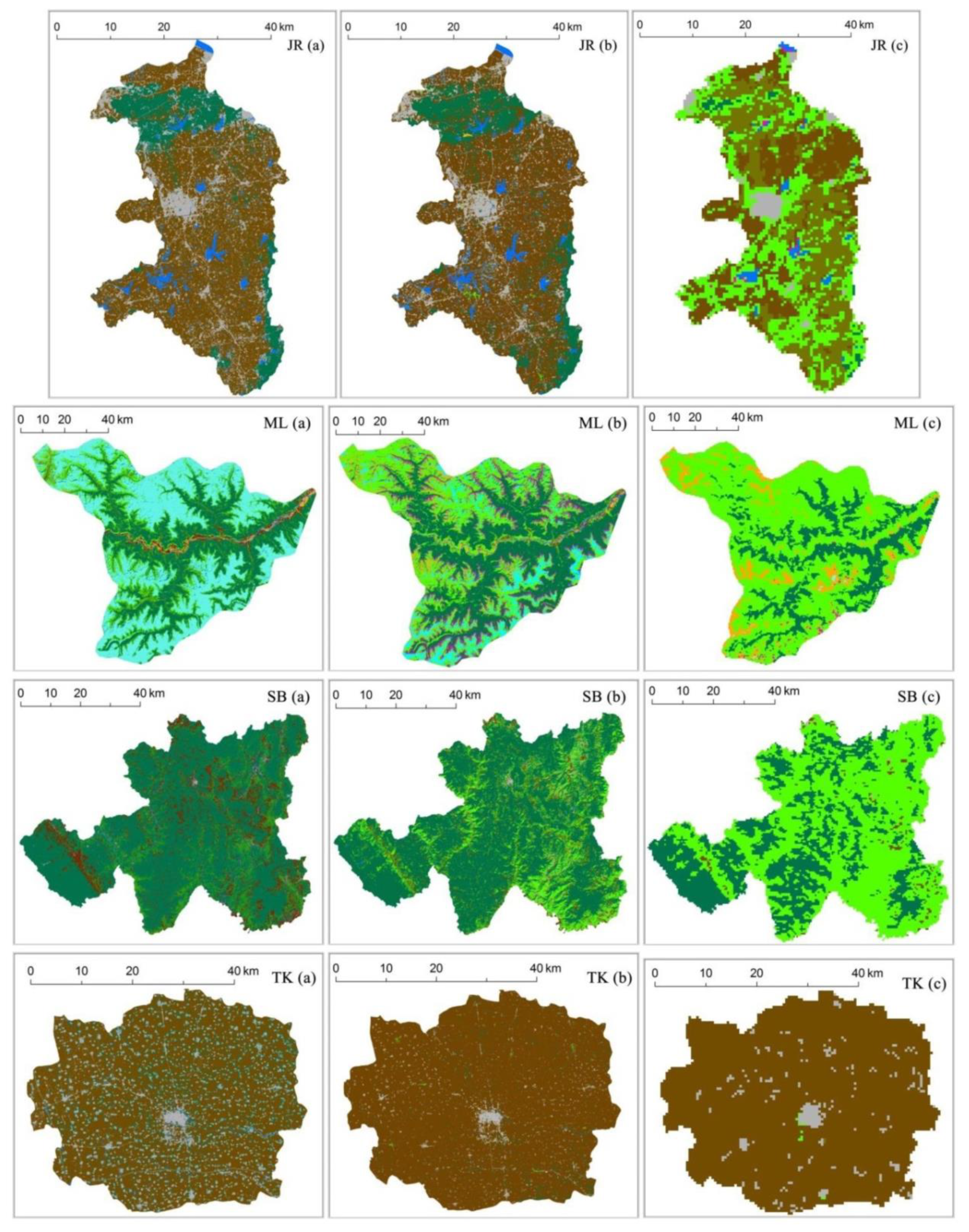
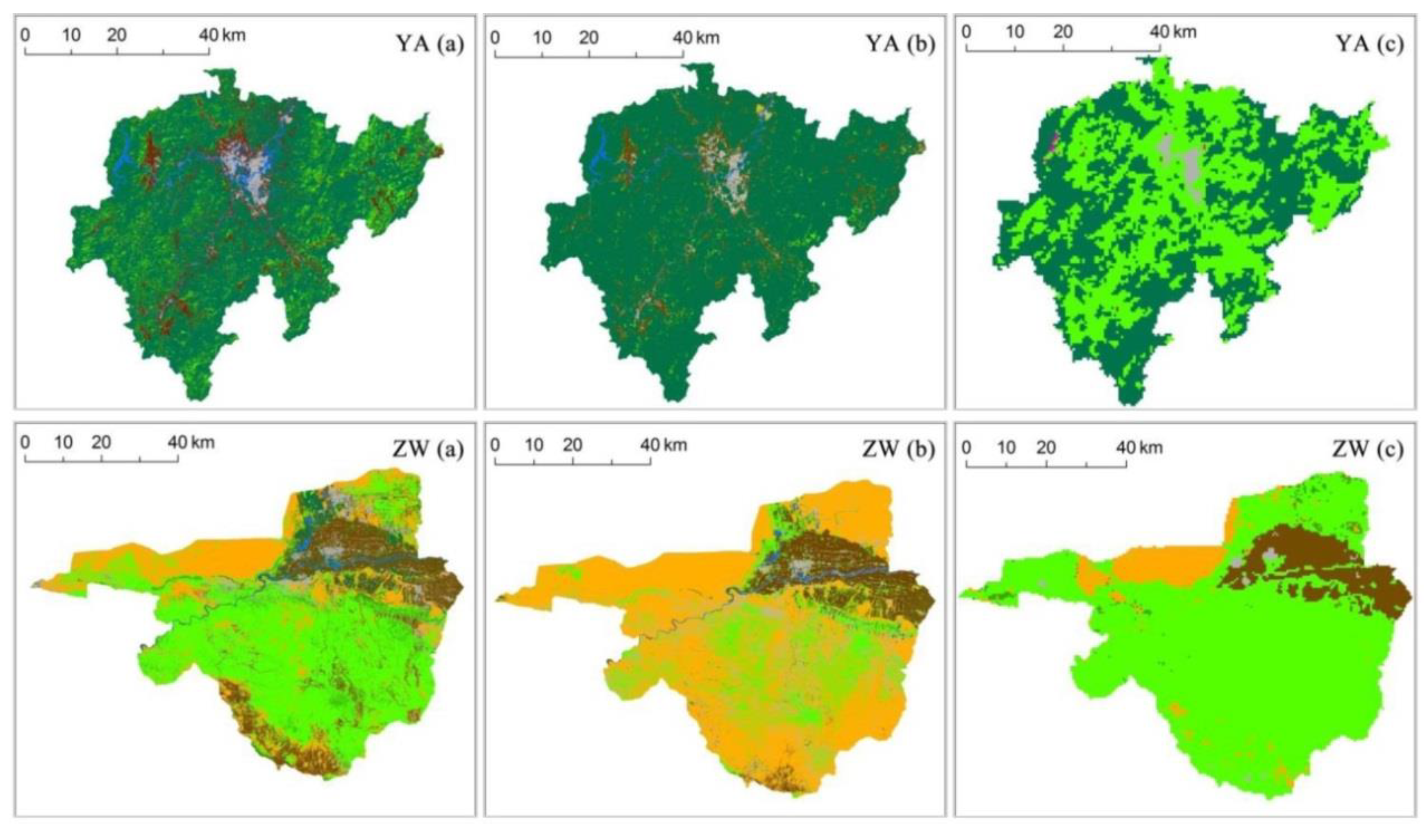
Figure 7 and Figure 8 compare the accuracy and results, respectively, of the optimal classifications with the existing land datasets, including FROM-GLC and MODIS LCT. Figure 7 shows that the newly produced data were more accurate than the FROM-GLC and MODIS LCT datasets in all regions. The mean accuracy for the area of our study, 84.4%, exceeded the accuracies of FROM-GLC and MODIS LCT, 64.0% and 42.5%, respectively. The error of FROM-GLC data was partly because the data were produced using images from around 2010 while the testing samples were based on images acquired in 2013. However, the difference of 20% was caused mainly by the different methods by comparing the Landsat OLI images from the two years.
On the whole, our data were similar to FROM-GLC data. The difference between FROM data and our data was its misclassification between natural vegetation and cropland in typical agro-pastoral regions like BLZ County and in southern hilly regions like SB County, where there were terraced fields. The MODIS LCT lost many land cover details because of its coarse spatial resolution compared with the classification data from our study (Figure 8). Misclassification between grass and forest was obvious in southern hilly areas such as parts of SB County and YA County in the MODIS LCT dataset.
5. Discussion
5.1. The Trait and Identification of Low-Accuracy Areas
The existence of low-accuracy areas is due to complex topography and/or heterogeneous land covers, so the locations of low-accuracy areas are relatively fixed. The low-accuracy areas are also similar for the LCC datasets derived from satellite images in different spatial resolutions. The spatial heterogeneity has caused many mixed pixels, which are the main error source for low spatial resolution classification data. Spatial heterogeneity is also the main reason for the SODS (the same object with different spectra) and DOSS (different objects with the same spectrum), which are two of the most important causes for low accuracy when the mid- and high-spatial resolution images are classified. Therefore, the low-accuracy areas extracted by this research can be used in other studies and land cover classifications.
In this paper, low-accuracy areas of China was extracted based on the accuracy assessment of 2010 MODIS LCT data. The reference data is a visually-interpreted regional land cover datasets with high accuracy. The MODIS global LCT data is one of the most popular LCC datasets and updated annually. The date of MODIS LCT data can match well with the date of the reference data. The reference data should have high accuracy, so visually-interpreted LCC maps are preferable, for example, the NLUD of China, the CORINE land cover of the Europe [30,41]. Datasets that are recognized by visual interpreting are also acceptable, such as the MRLC (now NLCD) of the USA [42]. Other high-accuracy datasets are also acceptable as long as its date is the same with the MODIS LCT data.
5.2. The Contribution of Existent Visually-Interpreted LCC Data in Classification Process
In the study, the MODIS 16-day EVI time series were used to decide the date of the applied image since it can find the optimal image that makes it easy to discriminate different vegetation types. In the process, the existent high-accuracy LCC data derived by visual interpretation (NLUD-C) provided a distribution of different vegetation types. This provides a basis for computing the regional average EVI of each vegetation type. The time range for the optimal image derived by the above method can be commonly used, as in a specific region the phenology for vegetation types is relatively stable.
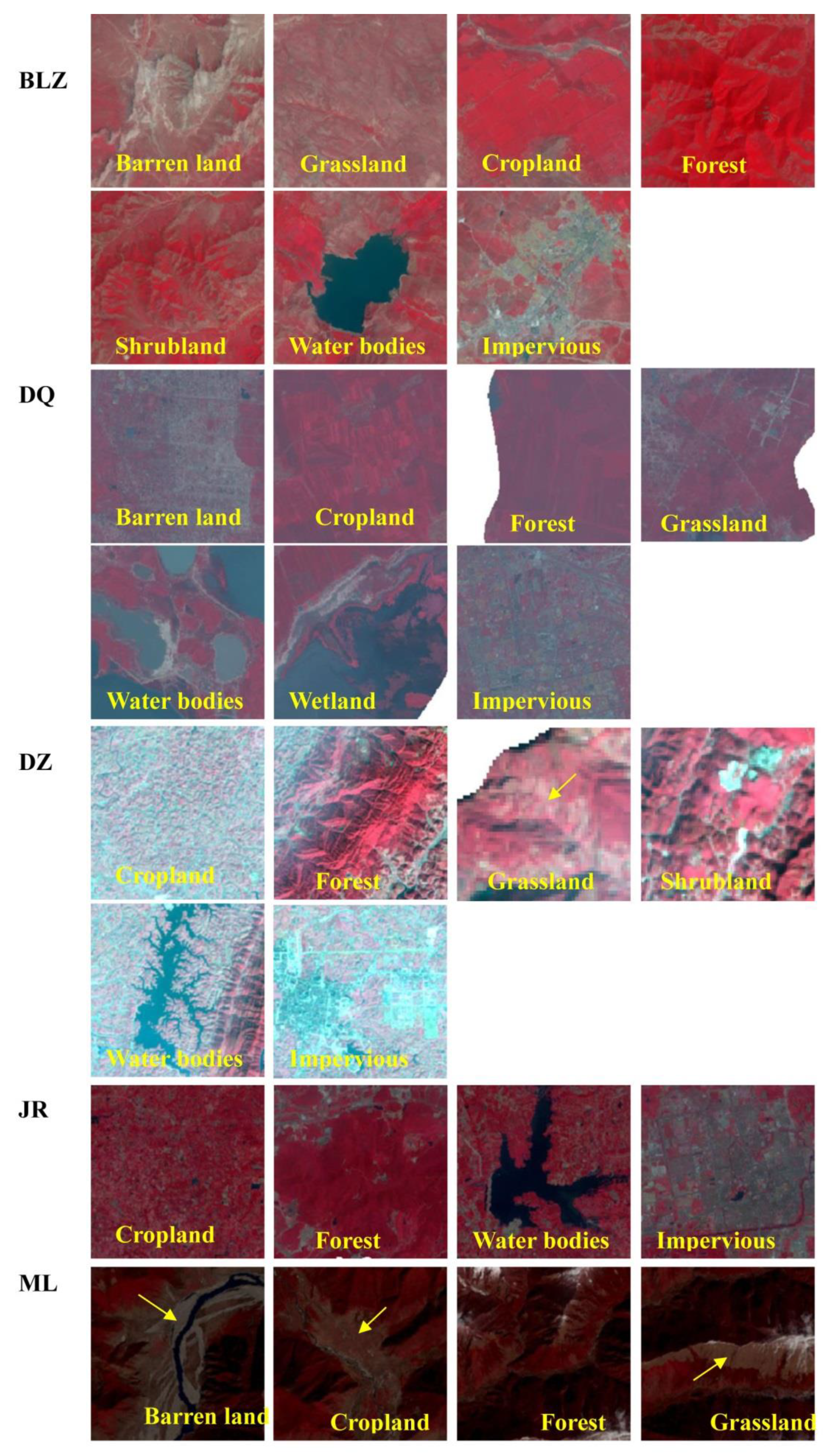
The representativeness of training samples is the most important factor that affects the LCC accuracy as the classifier is trained based on the selected training samples. Simply random selection cannot assure the representativeness of the training samples as the distribution of the land cover types is not even in a region. A divisional selection of training samples is extremely necessary in low-accuracy areas, since the spectral and topographical features for the same land cover type at different low-accuracy regions are very different (Figure A2). The existent high-accuracy land cover data (reference data) provided the divisions of different land cover types. The random selection of samples based on the divisions of different land cover types applied in the study improved the representativeness of training samples. The attributes (land cover type) of the training samples can be decided by visual interpretation and Google Earth.
5.3. Classification Algorithm and Features for the Low-accuRacy Areas in China
The SVM was found to be the first choice among the five algorithms for land cover mapping of low-accuracy areas, since it produced the highest accuracies in most regions. The good performance of SVM in land cover classification has been frequently noted in the past [9,25,42] but the over-fitting of SVM has rarely been discussed. We discovered that the dominant classes were easily misclassified as minority classes when the areal proportions of dominant classes exceeded greatly over the minority classes. For example, in YA where forest was the dominant class, the accuracy of SVM was decreased by the misclassification of forest. Over-fitting can be avoided as long as the training samples selected for dominant classes should include more pixels near the boundary.
In the study, it was implied that the impact of NDVI on accuracy was small and usually positive. Based on a meta-analysis, Khatami et al. [43] have also concluded that index creation of spectral bands like NDVI produces small improvements in accuracy. The three terrain features have usually been combined when they have been used as input data, whereas we separated them into single added features and discovered the negative effect of aspect on accuracy. Aspect should therefore not be used in LCC of low-accuracy areas. We suggest, however, that elevation and slope be used for areas where there are both plain regions and hilly regions. The reason is that crops are usually planted on plain regions because the water resources are plentiful, and the soils are fertile. However, elevation and slope tend to reduce accuracy in hilly areas where there are terraced fields, as the terraced fields are also cultivated on hillsides by farmers to augment food supplies. The remarkable effect of topographical information in classification makes it important to determine the terrain characteristics of different land cover types and choose suitable features before classification.
5.4. The Applicability and Limitation of the Integrated LCC Method
Several global LCC maps have been produced hitherto. Some of them have suggested the existence of low-accuracy regions in validation with testing samples, yet few of them has located the low-accuracy areas and studied them. This study provides a way for locating low-accuracy areas and an integrated method for the land cover mapping of low-accuracy areas. Different from most of the methods used in the global LCC maps, the integrated method optimizes all four procedures including image choosing, training sample selection as well as LCC algorithms and features, instead of one or two of them. This method is supposed to be used for global or large area land cover mapping when the low-accuracy areas are a significant factor leading to low-accuracy. The integrated method has improved the accuracy of low-accuracy regions so that it has exceeded a lot over the global LCC datasets derived from the same image source. Although the gaps between accuracies acquired by our method and by the visually-interpreted method still exists, our method has provided a valuable solution to narrow the gaps. The accurate visually-interpreted LCC data is necessary for locating low-accuracy areas and for the optimization of image choosing and training sample selection. If there was not any accurate LCC data are available, our method would not be suitable.
6. Conclusions
In the study, an integrated LCC method targeting low-accuracy regions in global LCC maps was developed. The low-accuracy regions were identified by an accuracy assessment of the MODIS LCT data. The integrated method ascertained the date of the optimal image, improved the representativeness of the training samples, by taking the advantage (high-accuracy) of visually-interpreted regional LCC datasets. It also selected the optimal classification algorithm and features for different regions in the low-accuracy areas by comparing the results from different algorithms and features.
We evaluated the integrated method in land-cover mapping of low-accuracy areas by using Landsat OLI imagery and topographical information as data source. China was taken as the study area and eight representative low-accuracy regions were examined. A classification result for each region was produced by the provided mapping method and outperforms the two precedent global land cover datasets (MODIS LCT and FROM-GLC). As the FROM-GLC also used the Landsat OLI imagery as data source, it implies that our method can improve the land cover mapping of low-accuracy areas.
Because of the existence of low-accuracy areas, it is critical to improve the quality of global land cover data. Much attention should be paid to the low-accuracy areas when mapping global land cover. In future studies, the methodology proposed in this study can be applied to global land cover mapping for improved accuracies.
Supplementary Materials
The following are available online at https://0-www-mdpi-com.brum.beds.ac.uk/2072-4292/11/15/1777/s1, Figure S1: MODIS EVI 16-day time series for all study sites, Figure S2: Location of randomly selected testing samples for validation for each study site.
Author Contributions
T.Z. conceived and designed this research and most of the analysis was done by T.Z. L.W. has participated in the writing and reviewing. Z.Z., Q.W. and X.W. have contributed to the data collection. L.Y. has given many good suggestions for modifying this article.
Funding
This work was funded by the “Strategic Priority Research Program” of the Chinese Academy of Sciences (XDA19070301) and the National Natural Science Foundation of China (Grant 91747201, 41571033). It was also supported by the International Partnership Program of the Chinese Academy of Sciences (131C11KYSB20160061) and the Top-Notch Young Talents Program of China.
Acknowledgments
We gratefully acknowledge the assistance of the Renewable Resource Division of Remote Sensing and Digital Earth, Chinese Academy of Sciences, for providing 2010 National Land Use Data of China. The manuscript has been edited carefully by two native-English-speaking professional editors from ELSS, Inc. ([email protected], https://www.elss.co.jp/en).
Conflicts of Interest
The authors declare no conflict of interest.
Appendix A
Figure A1.
The selected images (with “*”) for classification based on MODIS EVI time series. The grey grids stand for the time frame.
Figure A1.
The selected images (with “*”) for classification based on MODIS EVI time series. The grey grids stand for the time frame.

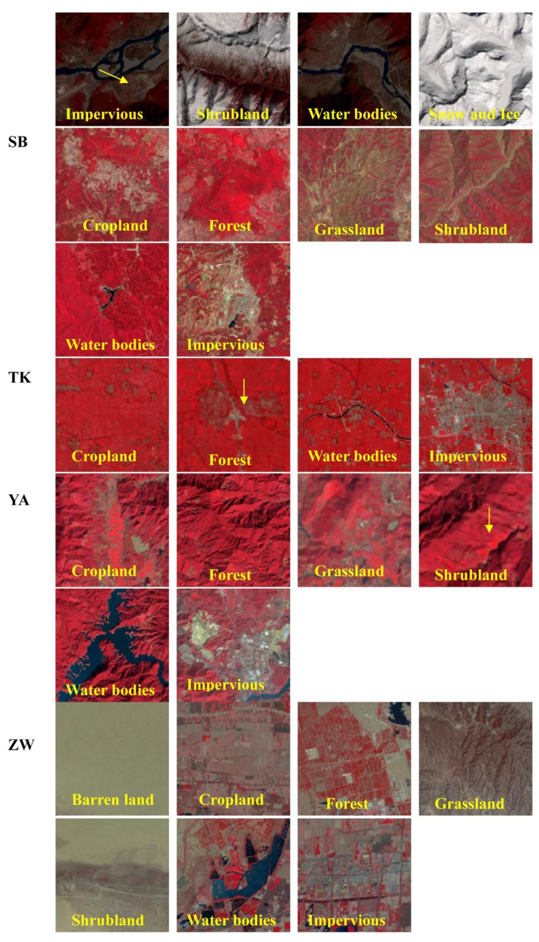
Figure A2.
Training samples that extracted from precedent high-accuracy land-cover map (CLUD) for all land cover types in the nine regions.
Figure A2.
Training samples that extracted from precedent high-accuracy land-cover map (CLUD) for all land cover types in the nine regions.


References
- Blaschke, T. Object based image analysis for remote sensing. ISPRS J. Photogramm. Remote Sens. 2010, 65, 2–16. [Google Scholar] [CrossRef] [Green Version]
- Foley, J.A.; Defries, R.; Asner, G.P.; Barford, C.; Bonan, G.; Carpenter, S.R.; Chapin, F.S.; Coe, M.T.; Daily, G.C.; Gibbs, H.K. Global Consequences of Land Use. Science 2005, 309, 570–574. [Google Scholar] [CrossRef] [PubMed] [Green Version]
- Grimm, N.B.; Faeth, S.H.; Golubiewski, N.E.; Redman, C.L.; Wu, J.; Bai, X.; Briggs, J.M. Global change and the ecology of cities. Science 2008, 319, 756–760. [Google Scholar] [CrossRef] [PubMed]
- Tian, J.; Zhang, B.Q.; He, C.S.; Yang, L.X. Variability in soil hydraulic conductivity and soil hydrological response under different land covers in the mountainous area of the Heihe River Watershed, Northwest China. Land Degrad. Dev. 2017, 28, 1437–1449. [Google Scholar] [CrossRef]
- Sellers, P.J.; Meeson, B.W.; Hall, F.G.; Asrar, G.; Murphy, R.E.; Schiffer, R.A.; Bretherton, F.P.; Dickinson, R.E.; Ellingson, R.G.; Field, C.B. Remote sensing of the land surface for studies of global change: Models–algorithms–experiments. Remote Sens. Environ. 1995, 39, 3–26. [Google Scholar] [CrossRef]
- Zhang, Z.X.; Chang, J.; Xu, C.Y.; Zhou, Y.; Wu, Y.H.; Chen, X.; Jiang, S.S.; Duan, Z. The response of lake area and vegetation cover variations to climate change over the Qinghai-Tibetan Plateau during the past 30 years. Sci. Total Environ. 2018, 635, 443–451. [Google Scholar] [CrossRef] [PubMed]
- Bontemps, S.; Defourny, P.; Bogaert, E.; Arino, O.; Kalogirou, V.; Perez, J. GLOBCOVER 2009—Products Description and Validation Report. Available online: http://due.esrin.esa.int/globcover/LandCover2009/GLOBCOVER2009_Validation_Report_2.2.pdf (accessed on 5 June 2016).
- Friedl, M.A.; Sulla-Menashe, D.; Tan, B.; Schneider, A.; Ramankutty, N.; Sibley, A.; Huang, X. MODIS Collection 5 global land cover: Algorithm refinements and characterization of new datasets. Remote Sens. Environ. 2010, 114, 168–182. [Google Scholar] [CrossRef]
- Gong, P.; Wang, J.; Yu, L.; Zhao, Y.C.; Zhao, Y.Y.; Liang, L.; Niu, Z.G.; Huang, X.M.; Fu, H.H.; Liu, S.; et al. Finer resolution observation and monitoring of global land cover: First mapping results with Landsat TM and ETM+ data. Int. J. Remote Sens. 2013, 34, 2607–2654. [Google Scholar] [CrossRef]
- Hansen, M.C.; Defries, R.S.; Townshend, J.R.G.; Sohlberg, R. Global land cover classification at 1 km spatial resolution using a classification tree approach. Int. J. Remote Sens. 2000, 21, 1331–1364. [Google Scholar] [CrossRef]
- Loveland, T.R.; Reed, B.C.; Brown, J.F.; Ohlen, D.O.; Zhu, Z.; Yang, L.; Merchant, J.W.; Defries, R.S.; Belward, A.S. Development of a global land cover characteristics database and IGBP DISCover from 1 km AVHRR data. Int. J. Remote Sens. 1999, 21, 1303–1330. [Google Scholar] [CrossRef]
- Tateishi, R. Production of global land cover data—GLCNMO. Int. J. Digit. Earth 2011, 4, 22–49. [Google Scholar] [CrossRef]
- Yu, L.; Wang, J.; Li, X.; Li, C.; Zhao, Y.; Gong, P. A multi-resolution global land cover dataset through multisource data aggregation. Sci. China Earth Sci. 2014, 57, 2317–2329. [Google Scholar] [CrossRef]
- Ran, Y.; Li, X.; Lu, L. Evaluation of four remote sensing based land cover products over China. J. Glaciol. Geocryol. 2010, 31, 391–401. [Google Scholar] [CrossRef]
- Zeng, T.; Zhang, Z.; Zhao, X.; Wang, X.; Zuo, L. Evaluation of the 2010 MODIS Collection 5.1 Land Cover Type Product over China. Remote Sens. 2015, 7, 1981–2006. [Google Scholar] [CrossRef] [Green Version]
- Townshend, J.R.G.; Justice, C.O. Towards operational monitoring of terrestrial systems by moderate-resolution remote sensing. Remote Sens. Environ. 2002, 83, 351–359. [Google Scholar] [CrossRef]
- Wulder, M.A.; White, J.C.; Goward, S.N.; Masek, J.G.; Irons, J.R.; Herold, M.; Cohen, W.B.; Loveland, T.R.; Woodcock, C.E. Landsat continuity: Issues and opportunities for land cover monitoring. Remote Sens. Environ. 2008, 112, 955–969. [Google Scholar] [CrossRef]
- Gomez, C.; White, J.C.; Wulder, M.A. Optical remotely sensed time series data for land cover classification: A review. ISPRS J. Photogramm. Remote Sens. 2016, 116, 55–72. [Google Scholar] [CrossRef] [Green Version]
- Giri, C.; Pengra, B.; Long, J.; Loveland, T.R. Next generation of global land cover characterization, mapping, and monitoring. Int. J. Appl. Earth Obs. Geoinf. 2013, 25, 30–37. [Google Scholar] [CrossRef]
- Hansen, M.C.; Loveland, T.R. A review of large area monitoring of land cover change using Landsat data. Remote Sens. Environ. 2012, 122, 66–74. [Google Scholar] [CrossRef]
- Irons, J.R.; Dwyer, J.L.; Barsi, J.A. The next Landsat satellite: The Landsat Data Continuity Mission. Remote Sens. Environ. 2012, 122, 11–21. [Google Scholar] [CrossRef] [Green Version]
- Drusch, M.; Del Bello, U.; Carlier, S.; Colin, O.; Fernandez, V.; Gascon, F.; Hoersch, B.; Isola, C.; Laberinti, P.; Martimort, P.; et al. Sentinel-2: ESA’s Optical High-Resolution Mission for GMES Operational Services. Remote Sens. Environ. 2012, 120, 25–36. [Google Scholar] [CrossRef]
- Lawrence, R.L.; Moran, C.J. The AmericaView classification methods accuracy comparison project: A rigorous approach for model selection. Remote Sens. Environ. 2015, 170, 115–120. [Google Scholar] [CrossRef]
- Pal, M.; Mather, P.M. Assessment of the effectiveness of support vector machines for hyper-spectral data. Future Gener. Comput. Syst. 2004, 20, 1215–1225. [Google Scholar] [CrossRef]
- Yu, L.; Liang, L.; Wang, J.; Zhao, Y.; Cheng, Q.; Hu, L.; Liu, S.; Yu, L.; Wang, X.; Zhu, P. Meta-discoveries from a synthesis of satellite-based land-cover mapping research. Int. J. Remote Sens. 2014, 35, 4573–4588. [Google Scholar] [CrossRef]
- Li, C.; Wang, J.; Wang, L.; Hu, L.; Peng, G. Comparison of Classification Algorithms and Training Sample Sizes in Urban Land Classification with Landsat Thematic Mapper Imagery. Remote Sens. 2014, 6, 964–983. [Google Scholar] [CrossRef] [Green Version]
- Clinton, N.; Yu, L.; Gong, P. Geographic stacking: Decision fusion to increase global land cover map accuracy. ISPRS J. Photogramm. Remote Sens. 2015, 103, 57–65. [Google Scholar] [CrossRef]
- Lesiv, M.; Moltchanova, E.; Schepaschenko, D.; See, L.; Shvidenko, A.; Comber, A.; Fritz, S. Comparison of Data Fusion Methods Using Crowdsourced Data in Creating a Hybrid Forest Cover Map. Remote Sens. 2016, 8, 17. [Google Scholar] [CrossRef]
- Perez-Hoyos, A.; Garcia-Haro, F.J.; San-Miguel-Ayanz, J. A methodology to generate a synergetic land-cover map by fusion of different land-cover products. Int. J. Appl. Earth Obs. Geoinf. 2012, 19, 72–87. [Google Scholar] [CrossRef]
- Zhang, Z.; Wang, X.; Zhao, X.; Liu, B.; Yi, L.; Zuo, L.; Wen, Q.; Liu, F.; Xu, J.; Hu, S. A 2010 update of National Land Use/Cover Database of China at 1:100000 scale using medium spatial resolution satellite images. Remote Sens. Environ. 2014, 149, 142–154. [Google Scholar] [CrossRef]
- Yang, L.; Homer, C.; Hegge, K.; Huang, C.; Wylie, B.; Reed, B. A Landsat 7 scene selection strategy for a national land cover database. In Proceedings of the IEEE 2001 International Geoscience and Remote Sensing Symposium, Sydney, Australia, 9–13 July 2001; Volume 1, pp. 1123–1125. [Google Scholar] [CrossRef]
- Piper, J. Variability and bias in experimentally measured classifier error rates. Pattern Recognit. Lett. 1992, 13, 685–692. [Google Scholar] [CrossRef]
- Van Niel, T.G.; McVicar, T.R.; Datt, B. On the relationship between training sample size and data dimensionality: Monte Carlo analysis of broadband multi-temporal classification. Remote Sens. Environ. 2005, 98, 468–480. [Google Scholar] [CrossRef]
- Shackelford, A.K.; Davis, C.H. A hierarchical fuzzy classification approach for high-resolution multispectral data over urban areas. IEEE Trans. Geosci. Remote Sens. 2003, 41, 1920–1932. [Google Scholar] [CrossRef] [Green Version]
- Breiman, L. Random Forest. Mach. Learn. 2001, 45, 5–32. [Google Scholar] [CrossRef]
- Cessie, S.L.; Houwelingen, J.C.V. Ridge Estimators in Logistic Regression. Journal of the Royal Statistical Society. Ser. C Appl. Stat. 1992, 41, 191–201. [Google Scholar] [CrossRef]
- Hsu, C.W. A Practical Guide to Support Vector Classification. Available online: https://www.researchgate.net/publication/288023219_A_Practical_Guide_to_Support_Vector_Classification (accessed on 5 June 2016).
- Landwehr, N.; Hall, M.; Frank, E. Logistic Model Trees. Mach. Learn. 2005, 59, 161–205. [Google Scholar] [CrossRef] [Green Version]
- Richards, J.A. Remote Sensing Digital Image Analysis, 5th ed.; Springer-Verlag: Berlin/Heidelberg, Germany, 2013; pp. 247–318. ISBN 13: 9783642300615. [Google Scholar]
- Mathur, A.; Foody, G.M. Multiclass and Binary SVM Classification: Implications for Training and Classification Users. IEEE Geosci. Remote Sens. Lett. 2008, 5, 241–245. [Google Scholar] [CrossRef]
- CORINE L and Cover. Available online: https://www.eea.europa.eu/publications/COR0-landcover#tab-related-publications (accessed on 1 July 2019).
- Vogelmann, J.E.; Sohl, T.L.; Campbell, P.V.; Shaw, D.M. Regional Land Cover Characterization Using Landsat Thematic Mapper Data and Ancillary Data Sources. Environ. Monit. Assess. 1998, 51, 415–428. [Google Scholar] [CrossRef]
- Khatami, R.; Mountrakis, G.; Stehman, S.V. A meta-analysis of remote sensing research on supervised pixel-based land-cover image classification processes: General guidelines for practitioners and future research. Remote Sens. Environ. 2016, 177, 89–100. [Google Scholar] [CrossRef] [Green Version]
Figure 1.
Distribution of nine study sites in China. The OA (overall accuracy) is the overall accuracy of every county in the accuracy assessment of MODIS LCT data. The OA of China averaged 64.62%. All counties in China were divided into two categories depending on whether their accuracies exceeded or were less than 64.62%. The counties with OAs <64.62% were classified as low-accuracy areas. The accuracies of study sites were listed in the brackets. TK was located in a high-accuracy area, whereas the other eight study sites (BLZ, DQ, DZ, JR, ML, SB, YA and ZW) were located in low-accuracy areas. The nine study sites were located in different eco-regions of China (Table 1).

Figure 2.
Flowchart of the optimization processes.

Figure 3.
Time-series of 16-day enhanced vegetation index (EVI) and Ed for the major land cover types in BLZ during 2013. Ed indicates the difference of EVIs between the main land cover classes (Equation (1)). The four dotted lines indicate the optimal times for image classification. Line “a” and line “b” indicate the peak values of the EVI for cropland, which was the dominant land cover type in BLZ. Line “c” is the EVI value that exceeded the peak EVI value minus 0.02. Line “d” indicates the peak value of Ed.

Figure 4.
Comparison among OAs of the five algorithms across the nine study sites with spectral bands as the only class features. “Mean” stands for the mean accuracy of all study sites in low-accuracy areas, with the exclusion of TK.
Figure 4.
Comparison among OAs of the five algorithms across the nine study sites with spectral bands as the only class features. “Mean” stands for the mean accuracy of all study sites in low-accuracy areas, with the exclusion of TK.

Figure 5.
Over-fitting caused by SVM (Support Vector Machine) at YA (Yong An City). Over-fitting that was caused by using SVM (a) and misclassification of forest at YA with spectral bands as classification features and SVM as classification algorithm (b). In panel (b), the first bar represents forest in the validation data. Different colors (other than green) in one bar indicate the percent of forest pixels that were misclassified as another land-cover type.

Figure 6.
Accuracy variations caused by adding new features to classification input on the basis of spectral bands. Variation is equal to classification accuracy of spectral bands and new features minus the accuracy of only spectral bands.
Figure 6.
Accuracy variations caused by adding new features to classification input on the basis of spectral bands. Variation is equal to classification accuracy of spectral bands and new features minus the accuracy of only spectral bands.

Figure 7.
Accuracy comparison between the classification of this study (OLI) and existing datasets (FROM-GLC and MODIS LCT). AVE is the mean accuracy of study sites in low-accuracy areas.
Figure 7.
Accuracy comparison between the classification of this study (OLI) and existing datasets (FROM-GLC and MODIS LCT). AVE is the mean accuracy of study sites in low-accuracy areas.

Figure 8.
Classifications results from different datasets. Classification of this study (a), classification data from FROM-GLC (b) and classifications from MODIS LCT (c).
Figure 8.
Classifications results from different datasets. Classification of this study (a), classification data from FROM-GLC (b) and classifications from MODIS LCT (c).


Table 1.
Characteristics of the selected study sites in low-accuracy areas of China.
| Study Site | Location | Area (km2) | Image (Path/Row) | Image Time |
|---|---|---|---|---|
| BLZ | Agro-pastoral zone | 6418 | 122/29 | 20140727 |
| DQ | Northeast Plain | 5065 | 119/28 | 20140722 |
| DZ | Sichuan Basin | 2083 | 127/39 | 20131202 |
| JR | Middle and Lower Yangtze Valley Plain | 1390 | 120/38 | 20130811 |
| ML | Southeast of Tibetan Plateau | 9045 | 136/40 | 20140119 |
| SB | Yunnan and Guizhou Plateau | 4114 | 130/43 | 20130614 |
| TK | North Plain | 1766 | 123/36 | 20130901 |
| YA | Southeast Hilly Area | 2944 | 120/42 | 20131201 |
| ZW | Inner Mongolia Plateau | 4529 | 130/34 | 20140601 |
Table 2.
Datasets used in this study.
| Dataset | Use for | Spatial Resolution (m) | Data Source |
|---|---|---|---|
| Landsat OLI | classification | 30 | www.glovis.usgs.gov/ |
| GDEM v2 | classification | 30 | www.reverb.echo.nasa.gov/ |
| MOD13Q1 | Image selection | 250 | https://ladsweb.modaps.eosdis.nasa.gov/search/ |
| FROM-GLC | Accuracy comparison | 30 | http://0-data-ess-tsinghua-edu-cn.brum.beds.ac.uk/ |
| MODIS LCT | Accuracy comparison | 500 | https://ladsweb.modaps.eosdis.nasa.gov/search/ |
Table 3.
Land cover classification system used in this study.
| Code | Name | Definition |
|---|---|---|
| 1 | Cropland | Land with cultivated crops growing on it in growing season |
| 2 | Forest | Natural or planted forests |
| 3 | Grassland | Natural or planted Grassland |
| 4 | Shrubland | Shrub cover identifiable in the image, having a texture finer than tree canopies but coarser than Grassland. |
| 5 | Wetland | Perennial or seasonal inundated land with hygrophytes growing on it. |
| 6 | Water bodies | All inland water bodies. |
| 7 | Tundra | Located at high mountains above tree line and high latitude regions with low height vegetation. |
| 8 | Impervious land | Primarily based on artificial cover such as asphalts, concrete, sand and stone, bricks, glasses and other cover materials. |
| 9 | Barren land | Vegetation is hardly observable, while dominated by exposed soil, sand, gravel and rock backgrounds. |
| 10 | Snow and ice | Distributed in the polar areas and high mountains. |
Table 4.
Numbers of testing samples for each land cover class.
| Study Site | BLZ | DQ | DZ | JR | ML | SB | TK | YA | ZW |
|---|---|---|---|---|---|---|---|---|---|
| The number of classes | 7 | 7 | 6 | 4 | 8 | 6 | 4 | 6 | 7 |
| Cropland | 141 | 173 | 311 | 282 | 40 | 91 | 340 | 69 | 82 |
| Forest | 90 | 30 | 135 | 105 | 205 | 296 | 30 | 339 | 30 |
| Grassland | 189 | 102 | 30 | 0 | 53 | 78 | 0 | 30 | 212 |
| Shrubland | 37 | 0 | 30 | 0 | 36 | 30 | 0 | 30 | 30 |
| Wetland | 0 | 30 | 0 | 0 | 0 | 0 | 0 | 0 | 0 |
| Water bodies | 30 | 48 | 30 | 30 | 56 | 30 | 30 | 30 | 30 |
| Impervious | 30 | 49 | 30 | 85 | 48 | 30 | 124 | 30 | 30 |
| Barren land | 30 | 82 | 0 | 0 | 33 | 0 | 0 | 0 | 106 |
| Snow and ice | 0 | 0 | 0 | 0 | 123 | 0 | 0 | 0 | 0 |
| Total | 547 | 514 | 566 | 502 | 590 | 555 | 524 | 528 | 520 |
Table 5.
Algorithm parameter values and source of codes.
| Algorithm | Abbreviation | Parameter Type | Values of Parameter | SOURCE |
|---|---|---|---|---|
| Maximum-likelihood classification | MLC | prior probability | The same for all classes. | ENVI |
| Logistic regression | LR | Log likelihood edge value | 0, 10-10, …,10-1, 1 | Weka |
| Logistic model tree | LMT | Minimal instances for splitting | 5, 10, 15, 20, 25, 30 | Weka |
| Weight trimming | 0, 0.01, …, 0.34, 0.35 | |||
| Support vector machine | SVM | Penalty factor C | 1, 10, 20, …, 300 | Libsvm |
| Kernel function Parameter | 0.1, 0.2, …,0.9, 1, 2, 3, …, 39, 40 | |||
| Random forest | RF | numFeature | From 1 to the number of features | Weka |
| numTrees | 20, 40, 60, 80, 100 |
Table 6.
Accuracy comparison among classifications from different combinations of class features. Spectral bands were used in every classification. Below the second row, the capital letter stands for a newly added class feature as input: N is NDVI, E is elevation, S is slope and A is aspect. The underlined values are the highest accuracies for all study sites.
| Classification Input | Classification Accuracy (%) | ||||||||
|---|---|---|---|---|---|---|---|---|---|
| BLZ | DQ | DZ | JR | ML | SB | TK | YA | ZW | |
| Spectral bands | 78.8 | 80.5 | 78.1 | 87.7 | 81.5 | 88.1 | 95.6 | 85.0 | 84.0 |
| N | 79.0 | 80.9 | 78.3 | 88.1 | 80.2 | 88.5 | 95.8 | 84.5 | 83.9 |
| E | 80.1 | 80.0 | 89.2 | 81.7 | 87.0 | 83.3 | 81.0 | ||
| S | 79.5 | 78.8 | 87.9 | 82.7 | 87.6 | 85.2 | 82.9 | ||
| A | 78.1 | 77.6 | 85.7 | 80.2 | 86.1 | 84.1 | 81.5 | ||
| NE | 79.2 | 82.7 | 89.4 | 83.2 | 87.8 | 82.8 | 81.2 | ||
| NS | 79.0 | 78.8 | 87.7 | 82.4 | 84.5 | ||||
| NA | 78.1 | 77.0 | 85.5 | 82.7 | 85.2 | 83.7 | 81.5 | ||
| ES | 79.5 | 80.2 | 89.4 | 81.7 | 86.0 | 82.2 | 80.4 | ||
| EA | 78.8 | 79.2 | 89.2 | 81.5 | 85.2 | 82.6 | 79.8 | ||
| SA | 78.1 | 77.9 | 87.1 | 82.0 | 85.8 | 84.5 | 81.7 | ||
| NES | 79.3 | 82.7 | 89.2 | 82.9 | 86.7 | 81.6 | 80.6 | ||
| NEA | 78.8 | 79.2 | 89.0 | 82.7 | 85.2 | 81.3 | 79.6 | ||
| NSA | 78.2 | 78.1 | 86.1 | 83.4 | 85.6 | 81.8 | 81.5 | ||
| ESA | 78.8 | 79.3 | 88.7 | 83.4 | 84.5 | 81.8 | 79.8 | ||
| NESA | 79.2 | 80.4 | 89.2 | 84.1 | 84.3 | 81.1 | 80.2 | ||
© 2019 by the authors. Licensee MDPI, Basel, Switzerland. This article is an open access article distributed under the terms and conditions of the Creative Commons Attribution (CC BY) license (http://creativecommons.org/licenses/by/4.0/).
Share and Cite
MDPI and ACS Style
Zeng, T.; Wang, L.; Zhang, Z.; Wen, Q.; Wang, X.; Yu, L. An Integrated Land Cover Mapping Method Suitable for Low-Accuracy Areas in Global Land Cover Maps. Remote Sens. 2019, 11, 1777. https://0-doi-org.brum.beds.ac.uk/10.3390/rs11151777
AMA Style
Zeng T, Wang L, Zhang Z, Wen Q, Wang X, Yu L. An Integrated Land Cover Mapping Method Suitable for Low-Accuracy Areas in Global Land Cover Maps. Remote Sensing. 2019; 11(15):1777. https://0-doi-org.brum.beds.ac.uk/10.3390/rs11151777
Chicago/Turabian StyleZeng, Tian, Lei Wang, Zengxiang Zhang, Qingke Wen, Xiao Wang, and Le Yu. 2019. "An Integrated Land Cover Mapping Method Suitable for Low-Accuracy Areas in Global Land Cover Maps" Remote Sensing 11, no. 15: 1777. https://0-doi-org.brum.beds.ac.uk/10.3390/rs11151777
Note that from the first issue of 2016, this journal uses article numbers instead of page numbers. See further details here.