Do Urban Functional Zones Affect Land Surface Temperature Differently? A Case Study of Beijing, China


1
Institute of Remote Sensing and GIS, Peking University, Beijing 100871, China
2
School of Geographical Sciences and Urban Planning, Arizona State University, Tempe AZ 85287, USA
*
Author to whom correspondence should be addressed.
Remote Sens. 2019, 11(15), 1802; https://0-doi-org.brum.beds.ac.uk/10.3390/rs11151802
Submission received: 6 July 2019
/
Revised: 17 July 2019
/
Accepted: 30 July 2019
/
Published: 1 August 2019
(This article belongs to the Special Issue Urban Heat Island Remote Sensing)
Abstract
:The non-uniformity of the relationships between urban temperature and landscape has attracted board attention. The non-uniformity in urban areas is reflected in the spatial landscape’s heterogeneity and the difference of socio-economic functions. The former is shown as the spatial differentiation of land-cover, land-use, landscape composition, and configuration, while the latter leads to the difference of the intensity of human activities and population density, which are closely related with anthropogenic heat emission. Therefore, this study introduces urban functional zones (UFZs) to express urban spatial heterogeneity. This study also attempts to comprehend urban heat island (UHI) effects and discloses the variability of urban surface temperature (LST)–landscape relationships in different kinds of UFZs. There are two main technical difficulties—how to characterize the spatial heterogeneity of UFZs and how to quantify non-uniform LST effects. A three-level variable system is established from their attributes, inner structures, and interrelationships to characterize UFZs and their LST effects hierarchically. Considering the multi-collinearity among high-dimensional variables, the Elastic Net regression method is selected for quantitative analysis. The experimental results reveal the deficiency of uniform LST analysis for heterogeneous urban areas and verify the variable relationships of LST-landscaped with different kinds of UFZs.
1. Introduction
Urban heat island (UHI) [1] refers to the atmospheric warmth of a city compared to its countryside. The UHI effect is closely related to population growth and climate change, which are two of the most serious environmental issues of the 20th century [2]. The causes, patterns, and intensities of the UHI effect are widely discussed for all urban areas [3]. Affected and modified by human activities, the urban land cover has been changed significantly and irreversibly, from natural soil and vegetation to man-made objects, like buildings, roads, and impervious surfaces [4]. Additionally, more heat and moisture are released from human and human activities in urban areas. These changes affect the material circulation and energy flow, especially the heat and water balance, making urban areas relatively warmer [5].
The conventional method of UHI studies is to simply compare the air temperature in urban and rural areas by observation sites. These sites are classified into urban and rural categories, but these classifications have some problems in practice. On the one hand, the urban–rural division is artificial. Urban and rural areas are essentially a continuum [6]. Therefore, we cannot compare the intensity of the UHI effect based on simple categorical labels. On the other hands, the city is not a homogeneous area, but a highly heterogeneous region. The spatial distribution of air temperature within the city is uneven. Therefore, UHI studies should focus on the temperature difference among different zones, not only the “urban-rural” temperature difference. There are already many discussions on zone-based classification.
Chandler [7] was the first to develop a climate-based landscape classification and divided Greater London into four local regions. Then, according to the vegetation and building characteristics, Auer [8] proposed a landscape classification with 12 meteorologically significant land uses. Ellefsen [9] derived 17 urban terrain zones (UTZs) from the geometry, street configuration, and construction materials to present city structures and materials, and Stewart [10] developed a logical landscape classification, called local climate zone (LCZ), to provide context for air temperature measurements. LCZs are homogenous units with uniform land-covers, structures, materials, and human activities, defined by the height/packing of rough objects or the dominant cover.
However, the non-uniformity in urban areas is reflected not only in the spatial landscape heterogeneity, but also in the difference of socio-economic functions, which can lead to differences in the intensity of human activities and population density, and then cause an unbalanced distribution of anthropogenic heat emission in urban areas. Social sensing is a new approach to understanding our socio-economic environments [11]. We can describe urban activities and classify the distribution of different socio-economic developments based on mobile phone-based sensor data [12], point of interest (POI) data [13], GPS trajectory data [14], and social media data [15]. The spatial differentiations of anthropogenic heat emission in different urban areas can be reflected by the socio-economic activities and their heterogeneity. In this study, we integrated both landscape information and socio-economic information (such as POIs) to divide the urban surface into six kinds of urban functional zones (UFZs)—commercial zones, residential districts, industrial zones, campuses, parks, and shanty towns [16,17]. UFZs represent the complexity of diverse land-cover objects with similar spatial landscape structures and socio-economic activities [18]. For the same types of UFZs, both spatial landscape structures and socio-economic activities are greatly uniform, but for different types of UFZs, they are not uniform. Figure 1 shows the samples of different kinds of UFZs with diverse landscape compositions and configurations. In the residential district (Figure 1b), the industrial zone (Figure 1c), and the park (Figure 1e), three vegetation patches with similar sizes, spectral features, and textures marked in the red boxes are surrounded by differentiated local environments, which would lead them respond differently to temperature change. Therefore, the focus of this study is to disclose how the non-uniformity of spatial landscape structures and socio-economic activities across different types of UFZs affect urban surface temperature (LST).
To disclose the variability of LST–landscape relationships in different types of UFZs, we have set the following objectives. The first objective is to give a complete and comprehensive climate-related description of UFZs based on a threefold understanding: a) As a highly-heterogeneous collection of ground objects, its landscape composition and configuration is differentiated; b) as an individual unit, it has some global properties; and c) as a part of the city, there are interactions among UFZs. Landscape composition refers to the variety and abundance of patch types, typically quantified using the proportions of land-cover types [19,20]. Different underlying surfaces, with their own radiation, thermal, and moisture properties, affect the local thermal environments differently and cause spatial variation of urban temperatures [5]. Landscape configuration refers to the spatial properties, arrangements, positions, or geometric complexity of entities within UFZs [21]. These configurations influence surface energy fluxes and result in the spatial differentiation of urban temperature [22,23]. They should be considered in this study but defined on the UFZ level. Meanwhile, we should be concerned about the configuration (i.e., building patterns) of buildings, which are the characteristic features in urban areas. The pattern of rough objects like buildings will change urban morphology and affect the air movement and wind field over the city [24], as well as the air temperature [25,26]. The importance of building patterns to the urban thermal environment was overlooked in previous studies [25,27,28,29,30] The attributes of UFZs and their interrelationships with other UFZs reflect the urban spatial heterogeneity at larger scales by regarding UFZs as a whole.
Second, the definition of the UFZ variable system uses an abundant set of surface climate properties to fully depict urban spatial heterogeneity, which introduces multi-collinearity among the variables. The conventional approaches in existing studies, like the correlation coefficient [31], ordinary least square (OLS) regression [32,33], and principal component analysis (PCA) [34], are no longer applicable. An approach to overcome multi-collinearity is required.
Third, UHI studies, without distinguishing non-uniformity of spatial landscape structures and socio-economic activities across the urban areas, may lead to doubtful results since these studies cannot accurately disclose the variations in LST–landscape relationships caused by urban spatial heterogeneity. To verify this assumption, this study attempts to model the relationship between LST and landscape separately based on the UFZ category. The factors affecting urban temperature vary based on the type of UFZ, and even the same variable would have different influences on urban temperature for different kinds of UFZs. Then, after being compared to the case that does not distinguish the differences between different UFZ categories, there might be some new discoveries in LST–landscape relationships.
Fourth, insight into the variations in LST–landscape relationships at the UFZ level can improve existing urban patterns and guide urban planning to cope with UHI effects and build an environment-friendly city.
In summary, three contributions are made in this research: (1) UFZs are introduced to UHI studies, considering the LST effects of both spatial landscape heterogeneity and the differences of socio-economic functions; (2) UFZs and their LST effects are characterized hierarchically by a three-level variable system, and the effects of buildings on LST are emphasized; (3) the experiment results reveal the deficiency of uniform LST analysis for heterogeneous urban areas and demonstrate the variability of LST–landscape relationships in different kinds of UFZs. These contributions are novel and crucial to UHI studies and can offer some references in urban planning and management.
2. Study Area and Data Preprocessing
2.1. Study Area
The study area is located in Beijing, China (116°15′40″E to 116°21′25″E, 39°56′15″N to 40°0′40″N) (Figure 2). The annual average temperature in the urban areas ranges from 11 ℃ to 13 ℃. The weather is dominated by prevailing southeasterly winds in summer and prevailing northwesterly wind in the winter. The wind conditions are also affected by the local micro-landform.
As the capital city of China, Beijing is highly-urbanized. The study area covers large urban regions (67.1 km2) and involves many typical ground objects in the urban ecosystem, including natural waterbodies with large areas, vegetation, farmland and harvested farmland, impervious surfaces (e.g., roads, parking lots, sidewalks), as well as various buildings whose size, height, and roof materials are completely different. As a mega-city in a mature period, the city has already been divided into distinct sub-regions by social functions. In this region, there are parks dominated by natural objects, campuses, commercial zones with skyscrapers, residential zones with plenty of regular buildings, industrial zones, and shanty towns. Different social functions determine the different landscape compositions and configurations. Highly differentiated urban functions intensify urban spatial heterogeneity and complicate LST–landscape relationships. Therefore, the hypothesis of this study can be fully verified in this strongly heterogeneous region.
2.2. Land Surface Temperature
For the urban thermal environment, air temperature data obtained from fixed observation sites are accurate but lack continuity, while remotely sensed thermal imagery can provide a time-synchronized dense grid of temperature data over a whole city. Therefore, satellite-derived LSTs are widely applied in studies of UHI effects and verified to closely correspond with UHIs [3].
In this study, LSTs were generated from the thermal infrared band (the spatial resolution is 60 m) of Landsat 7 Enhanced Thematic Mapper Plus (ETM+) imagery, which was acquired on the 4 November 2010 through the radiative transfer equation. The data were acquired in the daytime, during autumn, under cloud-free conditions. The original data were preprocessed using the Environment for Visualizing Images (ENVI) software, including radiometric calibration, atmospheric correction, cutting, and splicing. The striped noises of the imagery caused by the scan line corrector (SLC)-off were eliminated by the Gap-fill tool in ENVI.
To retrieve LST, land surface emissivity (ε) is computed by setting the research area into three main land surface features (water surface, town surface, and natural surface). Water surface only consist of waterbodies, and the town surface includes buildings and roads. The natural surface consists of vegetation and bare soil. The normalized difference vegetation index (NDVI) and vegetation fractional cover index (FC) are calculated to divide the study areas and estimate ε:
where b4 and b3 are the DN value of band 4 and band 3 of the Landsat 7 ETM+ image. The NDVI value between vegetation and bare soil indicate that the pixel is mixed with both vegetation and soil. Thus, we can describe the vegetation fractional cover of each pixel using the following formula:
where and are the NDVI value of the vegetation and the soil, respectively. According to the empirical formula of previous studies [35], we set the ε of the water surface pixel as 0.995. The ε of the town and natural surface are calculated by the following formulas:
where is the ε of the natural surface and is the ε of the town surface.
The radiance received by the satellite sensor with brightness temperature T, is composed of three parts—the ground radiance after atmospheric absorption, the downwelling path radiance reflected by the ground, and the upwelling path radiance:
where is the surface emissivity, is the ground radiance, is atmospheric transmittance, is downwelling path radiance, and is upwelling path radiance [36]. Then, can be expressed as
, and can be obtained from the NASA website (https://atmcorr.gsfc.nasa.gov/) according to the time and position of image acquisition [37].
2.3. Land Cover Data
Land cover data were produced via Worldview-II image with eight bands whose spatial resolutions for the panchromatic and multispectral bands are 0.5 m and 2 m, respectively. These data were acquired on 8 November 2010, the same time phase as the LST data. An object-based image analysis method with adaptive scale estimation [40] was employed to recognize the six classes: water, vegetation (VEG), buildings (BLD), bare soil, roads, and shadows. To guarantee the accuracy of the following experiments, land cover map should be visually verified and manually corrected by ground survey data.
2.4. Urban Functional Zones
Based on urban spatial heterogeneity, the multi-level aggregation method was proposed to aggregate land-cover objects spatially into UFZs, based on the visual features of land-cover objects (spectral, geometrical, and textual features) and their spatial distribution patterns (neighboring and disjoint relations) [16]. We then classified the UFZs into six classes by incorporating socio-economic information (e.g. educational institutes, commercial points, residential buildings, parks, companies, and public services) with the hierarchical semantic cognition method [17]. Finally, based on the land cover map, we divided the study area into six classes of UFZs: commercial zones (CZ), residential districts (RD), industrial zones (IZ), campuses, parks, and shanty towns (ST). In order to ensure the validity of the experimental conclusions, the UFZ map was carefully verified by visual interpretation and field trips. The misclassification of UFZs should be manually corrected. The LSTs of UFZs are derived from the UFZ map and LST data. For each UFZ, its LST was estimated by the average temperature of the pixels within the UFZ.
Moreover, due to the inconsistency in resolution and the image extent between the LST map and UFZ map, some UFZs with extremely small areas, or those near the boundary of the whole image, have inaccurate data or no temperature data. These are regarded as "invalid zones" and excluded from the subsequent analysis.
3. Methodology
The general process includes data acquisition, data preprocessing, modeling, and analysis (Figure 3). First, generate thematic maps (LST map, land cover map, UFZ map, and building pattern map) from original images. Second, derive the dependent and independent variables. The LST map and UFZ map combine to produce the LST for each UFZ as the dependent variable. The independent variables are organized into a three-level variable system derived from the land cover map, UFZ map, and building data. Third, Elastic Net regression [41] is used to model the LST–landscape relationships. To evaluate the influence of UFZs on LST, seven models were built, out of which six single models consider each type of UFZ separately, and the seventh mixed model considers all kinds of UFZs together. The selected models are compared and evaluated to answer two questions: do different kinds of UFZs have different LST effects? How does one quantify the differences caused by different kinds of UFZs?
3.1. Definitions of Explanatory Variables
As an expression of urban spatial heterogeneity, UFZs help to express the geographic differentiations in LST–landscape relationships. The landscape’s composition and configuration within UFZs dominate urban spatial heterogeneity and are the originators of the geographic differentiation of LST–landscape relationships. The LST effects of building patterns also cannot be ignored because of their major influence on local air movement, which can change the local LST field. From a global perspective, LST has strong spatial dependence, and no UFZ interacts with the LST separately in space. The LST of one UFZ would be affected by its neighboring UFZs. In summary, LST variable systems were extended to three levels in this study: the structure of UFZs (i.e., landscape composition and configuration within UFZs), the attributes of UFZs, and the interrelationship between UFZs (Figure 4). The specific definitions of the select variables at each level are as follows.
The variables at the first level are intended to describe the landscape composition and configuration in UFZs. Thus, they are computed based on the polygons of UFZs and include two parts. The first part refers to landscape characteristics, which describe the categories, abundance, and spatial distribution of every ground object type inside the UFZs. Four composition and configuration variables potentially relevant to LST [42] are selected (Table 1). It should be noted that although these variables are the same as those in previous studies, they are defined based on different spatial units. Traditionally, landscape composition and configuration variables are defined based on a moving window centered at each pixel. However, the variables of neighboring pixels are strongly correlated because the moving windows of the neighboring pixels have large overlapping areas. The correlation of the variables in this situation may lead to a misunderstanding of LST-landscape relationships. In this study, these variables are computed for every ground object type using the polygons of UFZs instead of pixels. There are six land-cover classes. Thus, the four variables can be expressed by a vector with a dimension of 4 × 6. Since the distribution of ground objects in every UFZ type is unbalanced, the variables of rare classes should be excluded for each UFZ type. For example, there is no waterbody in most shanty towns, so it is unnecessary to put the variables for water into the variable system of shanty towns. There are still some variables that play a limited role in explaining LST effects, so further variable selection is still needed.
The second part of the variables at the first level is for building patterns. As the unique ground object type in urban areas, building patterns related to the spatial distribution of buildings are also an important part of the UFZ structure. Building patterns can affect the LST by changing the local air movement and wind field. Buildings in rows tend to form wind corridors that can accelerate the air flow and cool the urban surface, while buildings in scattered distribution can make the air flow stick and may engender a high local LST. To incorporate the influences of building patterns, a set of variables is designed to measure building patterns (Table 2). The number of buildings is considered to embody the density of buildings in UFZs and measure to what extent buildings affect the LST in UFZs. Other four variables describe whether buildings are in regular distribution, which is a precondition of the wind-corridor effect. The regular distribution is measured in two aspects: the similarity of the shapes and the regularity of the arrangement. The former aspect is measured by the area standard deviation of buildings. To quantify the latter aspect, the conception of a building chain is introduced. A building chain refers to the collinear pattern of buildings formed by buildings with a similar proximity, continuity, and spatial directionality. This approach [43] is employed to extract building chains (Figure 5b) from the building vector data (Figure 5a). The number and length of building chains give a quantitative description of the wind-corridor effect, while the ratio of buildings in chains to the total number of buildings measures whether the distribution of buildings in UFZs is regular.
Three UFZs are taken as examples to illustrate how the five variables (Table 2) describe building patterns (Figure 5c–e). In Figure 5c, there is obviously only one kind of building with the same size and shape. Buildings are arranged orderly, forming a grid. In Figure 5d, the building pattern is quite different from that in Figure 5c. There are two kinds of buildings in Figure 5d, one with similar shapes and a regular arrangement, and the other with a complex shape and very high. Moreover, buildings in Figure 5e have no clear distribution pattern but are densely clustered. These buildings all have different sizes and roof materials.
It should be noted that number of buildings in Figure 5c,d is far less than those in Figure 5e. Since the three UFZs in Figure 5c–e have the same area, the number of buildings can directly reflect the crowdedness of the buildings. The similarity of buildings in the region can be measured by their size, shape, and distribution. Among them, the area similarity is the most direct measurement. A small area standard deviation of buildings (BLD-AREA-SD) value means small variation in building areas, while a large BLD-AREA-SD value means large variation. Based on the measurement of the shape similarity, the buildings in a chain/network distribution can be extracted. There are seven horizontal and vertical building chains in Figure 5c, forming a regular grid structure. Two vertical building chains can be extracted from Figure 5d, while no buildings are lined up and no building chains can be extracted in Figure 5e. The number and length of building chains can quantitatively reflect how many buildings are regularly distributed in a UFZ. However, the numbers of buildings in different UFZs are different. The regularity of buildings in a UFZ should be measured by the relative number of orderly arranged buildings and all buildings, that is, the variable for the ratio of buildings in chains to the total (RB). The higher the value of RB, the higher the proportion of buildings in regular layout is.
The variables at the second level are related to attributes of UFZs (Table 3). At this level, each heterogeneous UFZ unit is regarded as a whole. Compared with variables at the first level trying to explain the LST differentiation within a UFZ, the variables at the second level tend to determine the LST differences among UFZs. Basic attributes like area, perimeter, and shape index are selected to describe the UFZs themselves. Heterogeneity among UFZs is characterized by aggregated and diverse properties. The Contagion Index (CONTAG) measures the aggregated properties of the entire UFZ without differencing the separated patches inside it. Shannon’s Diversity Index (SHDI) and Simpson’s Diversity Index (SIDI) are used to measure diversity in a UFZ. They have different application conditions, and further selection should refer to the specific circumstance.
The variables at the third level aim at describing the interrelationships between spatially neighboring UFZs. First-order adjacency is a simple and direct expression of neighboring relations. Neighboring UFZs are defined as UFZs with overlapping edges. The proportion of the overlapping edge between a UFZ and its neighboring UFZs are summarized for every UFZ type to embody the influence of every UFZ type on the target UFZ (Table 4).
The variables of building patterns and the variables describing the relationship between neighboring UFZs are calculated using a software package developed by our research team, while others are calculated by the Fragstats software [44].
3.2. Modelling for Different Kinds of UFZs Using Elatic Net Regression
Urban spatial heterogeneity produces remarkable differences among UFZs. It is crucial to find the unique effects on the LST for UFZs with totally different structures, functions, and spatial contexts. The same type of UFZs often have similar attributes, inner structures, and interrelationships. Thus, the heterogeneity among the same type of UFZs is much smaller, such that they might share similar effects on the LST. However, the various kinds of UFZs significantly differ in their attributes, inner structures, and interrelationships. Thus, the heterogeneity among different kinds of UFZs is large, such that they have different effects on the LST.
To evaluate the spatially non-uniform LST–landscape relationships, this study designs seven models (Table 5). Model-CZ, Model-RD, Model-IZ, Model-C, Model-P, and Model-ST, which are referred to as single models in this study. These models are designed to analyze the LST–landscape relationship for each UFZ type, while Model-A, which is referred to as a mixed model in this study, considers all UFZs equally and does not differentiate the effects of different kinds of UFZs on the LST. A comparison of the mixed model with six single models can correctly explain the spatially non-uniform LST–landscape relationships.
Due to the multi-collinearity problems among independent variables, widely-used linear models [32,33] are not functional here. To solve this issue, regression shrinkage methods are introduced in this study by imposing a penalty on the size of coefficients. We use Elastic Net Regression [41] as the fitting method, a combination of Ridge Regression (Tikhonov regularization) [45] and LASSO (Least Absolute Shrinkage and Selection Operator) [46]. The loss function of Elastic Net Regression is
The penalty constraint term combines L1 regularization and L2 regularization. Therefore, Elastic Net combines the advantages of both Ridge and LASSO. First, it inherits the stability of Ridge and has no requirement for the sample size and dimensions of the variable system. Second, it can deal with multi-collinearity. Due to L2 regularization, collinear variables that contribute to the model can all be reserved in the variable selection process and automatically assigned a reasonable weight. Third, it can automatically achieve variable selection like LASSO. These superior characteristics made Elastic Net match the research requirements and be chosen as the regression method in this study. The parameters of regression, Alpha and L1_Ratio, are determined by K-fold cross-validation.
All the variables need to be standardized with zero mean and unit variance before the regression. Standardized model coefficients benefit both comparing the coefficients of different variables in the same model and comparing the coefficients of the same variables in different models. It can also provide insights into the different effects of different variables in the same type of UFZs and the different effects of the same variable in different kinds of UFZs. Moreover, due to the universal relationships between the LST and the independent variables in the seven models, the variables affecting the LST should be different. As a result, the dependent variables explaining LST–landscape relationships should be further selected for the seven models separately (Figure 3c).
For all the variables defined in Section 3.1, we calculate their correlation coefficients with LST for each model separately. The interactions among variables are not considered at this moment. The only concern is the significance of the relationship between each variable and LST. The variables significantly correlated with LST (Pc < 0.05) are chosen as the explanatory variables. The Elastic Net model can perform the variable selection during model fitting. That is, the regression coefficients of the variables that have limited effects on LST will be set as zero. The remaining variables that have significant effects on LST will be kept. To compare with existing studies without considering the landscape heterogeneity of UFZs, the same selection is conducted for the mixed model (Model-A) to verify whether there is a spatially uniform LST–landscape relationship in urban areas.
3.3. Model Evaluation
Elastic Net is not a statistical regression method but a type of machine learning algorithm. Therefore, both variable selection and regression fitting are different from the statistical regression methods judged by the significance test. The variables with significant influences are selected directly during fitting of the ridge trace. Therefore, this section will no longer discuss the significance of variables and models but evaluate the models in terms of the goodness of fit and spatial autocorrelation of the model residual.
1. The goodness of fit evaluation. The coefficient of determination, denoted by R2, is a statistic that will provide some information about the goodness of fit of a model. Its general definition is
where SSR means the sum of squares of the residuals, while SST means the total sum of squares. In regression, R2 is a statistical measure of how well the model approximates the real data points. R2 ranges from 0.0 to 1.0. An R2 of 1.0 indicates that the model perfectly fits the data. The larger the R2, the better the model.
2. Spatial autocorrelation evaluation of model residuals. The model residuals reflect the difference between the model predicted and the real values. Spatial autocorrelation refers to the potential interdependence among the values of neighboring objects led by the effects of spatial interaction and spatial diffusion and measured by Moran’s I (Index). Moran’s I ranges from -1.0 to 1.0.
The model residuals with no spatial autocorrelation will follow random spatial distribution, indicating that the model is well fitted. Positive spatial autocorrelation implies that similar values cluster together, while negative spatial autocorrelation suggests that dissimilar values cluster together. Two evaluation methods both show that the model lacks interpretive ability. Thus, more variables should be included, or the model itself needs to be modified.
4. Results
4.1. Data Preprocessing Results
The study area is classified into the six land cover types: water, vegetation, buildings, bare soil, roads, and shadows (Figure 6a). The accuracies of land cover for the individual types range from 85.6% to 95.0%, and the overall accuracy is 92.4%. Based on the land cover map, we divided the study area into six classes of UFZs (Figure 6b), with an accuracy of 89.3%. After visual verification and manual correction, we estimate LST for each UFZ. The results of LST retrieval show that LSTs in the whole study area range from 5.11 ℃ to 25.62 ℃, and the average LST is 16.20 ℃ (Figure 6c). For each UFZ, the LST ranges from 11.55 ℃ to 19.55 ℃ (Figure 6d). Finally, there are 374 valid UFZs, and their detailed information is as follows (Table 6).
4.2. Model Fitting and Performances
Due to the heterogeneity of UFZs, the results of model fitting vary hugely. For each model, the model parameters (Alpha and L1_Ratio) are set by K-fold cross-validation to achieve the best model fitting (Table 7). After modeling, an evaluation of the models’ results is conducted to check if these models are reliable and worth investigating in the future. In this study, the models are evaluated by the goodness of fit and spatial autocorrelation of the model residual.
The goodness of fit of the seven models is listed in Table 8. The values of of all the seven models are above 0.4, while the goodness of fit is low in some models for two reasons. One is caused by the heterogeneity among UFZs, and the other is that the penalty constraint term of the regression shrinkage methods that reduce the goodness of fit to keep the model stable. Model-A and Model-CZ have a low goodness of fit, since they are based on highly heterogeneous units. In contrast to parks with a unified style and residential zones with regular building patterns, commercial zones lack both unified styles and spatial patterns, not to mention the more complex UFZs in Model-A, which includes different kinds of UFZs. As for the relatively homogeneous models, like Model-IZ and Model-ST, their performances are much better, as they have large values of (0.94 and 0.75, respectively). This validates the necessity of modeling the LST–landscape relationships for each UFZ category.
Before modeling, a spatial autocorrelation analysis of the LST is first conducted. For LST, the Z-value of Moran’s I is 5.66 and the P-value is 0.00, indicating that the LST has a strong spatial autocorrelation and has a significantly clustered distribution. If the model can accurately explain the LST–landscape relationship, the model residuals should no longer show spatial autocorrelation but random distribution. The autocorrelation indices of the seven models are shown in Table 9.
The Z-value (3.43) of Model-A indicates that the residuals are still significantly auto-correlated. As a result, the mixed model (Model-A) is weak and inappropriate to explain the LST–landscape relationship. In contrast, the spatial autocorrelations of the residuals are weakened to varying degrees in six single models. The model residuals of industrial zones, campuses, parks, and shanty towns are not auto-correlated, indicating that these models perform well. The model residuals for commercial zones and residential districts show a tendency toward aggregation, but their aggregation degree is much weaker than the LST itself, owing to the good model fittings. In conclusion, in terms of the spatial autocorrelation of the residuals, the six single models for each UFZ type explain the LST–landscape relationship to varying degrees, and the coefficients of explanatory variables can be trusted. The performance of the mixed model (Model-A) is poor, but it still partly reflects the general laws in the urban areas and reveals that different UFZ kinds may have different LST effects and need to be modelled and analyzed separately.
4.3. Modeling Results
There are 41 variables at the three levels defined in Section 3.1. that might have potential associations with LST. After two rounds of variable selections, the final independent variables of the seven models vary greatly in both numbers (Table 10) and categories of variables (Table 11). Model-CZ has only eight independent variables that affect LST significantly. These variables are small in number due to the complicated and inexplicable LST effects caused by high spatial heterogeneity in commercial zones, leading to the poor performance of Model-CZ. The mixed model and other five single models have more variables, ranging from 14 to 20, but the categories of the variables and their coefficients vary greatly. The values in Table 11 are the coefficients of the chosen variables in the corresponding model.
4.4. Result Analysis of the UFZ Level
The variables of UFZs describe the basic attributes of the UFZs, landscape composition, and configuration within UFZs, as well as the interrelationships between neighboring UFZs. First, as the basic attributes of UFZs, area, perimeter, and SI are only included in Model-A and Model-P, but not in the other five single models. In Model-A, the coefficient of area (−0.04) suggests that the areas of UFZs are negatively related to the LST, while perimeter and SI are regarded to have minimal effects on LST, as their coefficients are set as 0.0. In Model-P, the coefficients of area (−0.16), perimeter (−0.02), and SI (−0.02) indicate that a large area, large perimeter, and complex shape could reduce the LST in parks.
Second, CONTAG embodies the distribution of patches within UFZs. A greater CONTAG value, which signifies more clustered patches, will lead to a lower LST in residential districts and parks, with the negative coefficients (−0.10 and −0.12) in Model-RD and Model-P respectively. However, in shanty towns, a greater CONTAG value indicates a stronger heating effect, with the positive coefficient (0.07) in Model-ST. In addition, the LSTs in commercial zones, industrial zones, and campuses are not affected by CONTAG.
Third, the diversity of the patches in the UFZs is measured mainly by SIHI and SDHI. The coefficients of SIHI in Model-CZ, Model-IZ, and Model-ST are −0.04, −0.05, and −0.03, respectively. The coefficients of SDHI in Model-CZ and Model-ST are −0.06 and −0.06, respectively. Moreover, these two variables are not significant in Model-A, Model-RD, Model-C, and Model-P. The negative coefficients show the patch diversity in the three UFZ types (i.e., commercial zones, industrial zones, and shanty towns) is negatively related to the LST, which can alleviate the increasing of LST.
Lastly, the results indeed show that the LST of a UFZ is greatly affected by its neighbors. UFZs might have heating or cooling effects on the neighboring UFZs, depending on the adjoined UFZ types. Like parks, the coefficient of Adjacency-P in Model-RD (−0.09) shows that the LST will decrease in residential districts adjoined to parks, while the coefficient of Adjacency-P in Model-C (0.03) indicates that the LST will increase in campuses adjoined to parks. Among these UFZ types, shanty towns have the most significant impact on the LST of adjoined UFZs. Table 11 shows that adjoining to shanty towns is not a good thing for almost all UFZ types. The positive coefficients of Adjacency-ST in the models, except for Model-C, reflect the positive relationships between the adjacency and the LST. However, neighboring campuses and shanty towns can reduce the LST for each other, embodied by the negative coefficients of Adjacency-ST in Model-P (−0.04) and Adjacency-P in Model-ST (−0.08). Moreover, in the interrelationship analysis (adjacent to its own type of UFZs) no longer reflects the adjacency relationship but the effect of size. Two adjacent UFZs can be regarded as a larger one. For residential districts, campuses, and parks, the adjacency variables of their own type are all negative (−0.03, −0.01, and −0.09), showing the cooling effects in different degrees. On the other hand, two adjoining shanty towns will both increase their LSTs, as revealed by the coefficient of Adjacency-ST in Model-ST (0.08).
4.5. Result Analysis of Land-Cover Level
The land-cover types contained in each UFZ are similar, but due to the differences in landscape composition, configuration, and human activities, the same land-cover type may have different LST effects and intensities on different kinds of UFZs. Next, we will show the different roles of six land-cover types in different models.
1. The variables of buildings. Four basic variables (i.e., BLD-ED, BLD-IJI, BLD-PD, and BLD-PLAND) depict the attributes of buildings the same as the attributes of other ground objects. Five more variables are added to characterize their spatial patterns, including the area standard deviation of buildings (BLD-AREA_SD), the number of buildings (NB), the number of building chains (NC), the length sum of all the chains (LC), and the ratio of buildings in chains to the total (RB).
From the results of each model, the LST effects of buildings are complex and diverse. The effects of buildings are most significant in the residential zones. There are five building variables significantly related to the LST, while commercial areas and parks have only one related variable.
In Model-A, the BLD-AREA_SD and BLD-PD tend to increase LST. For commercial zones, the LST is only increased by BLD-AREA_SD. For industrial zones, BLD-ED, BLD-PLAND, and NB are all positively related with the LST. Conversely, variables about buildings in Model-C and Model-P play a part in cooling the LST. The result of Model-C shows that BLD-AREA_SD and BLD-PLAND have a negative association with the LST in campuses, and the result of Model-P shows that NB is the only significant variable of the LST that shows parks with more buildings to be cooler.
In Model-ST, the impact of buildings on LST mainly emerges from three aspects: BLD-AREA_SD, BLD-PLAND, and BLD-IJI, with coefficients 0.05, 0.01, and −0.01, respectively. The former two are positively related with the LST, and the last one is negatively related with the LST. On the other hand, the absolute value of the coefficients of the last two (0.01 for BLD-PLAND and −0.01 for BLD-IJI) are very small, indicating the weakness of their influence.
The results of Model-RD show that the LST of residential districts is greatly influenced by the variables of buildings. The coefficients of BLD-AREA_SD (−0.04) and BLD-PLAND (−0.04) reflect their cooling effects while the coefficients of NB (0.13), NC (0.04), and RB (0.01) show that these variables have heating effects on LST.
2. The variables of vegetation. In most models, VEG-IJI has a negative relationship with LST and embodies the dispersion of vegetation. In Model-A, Model-CZ, Model-RD, Model-IZ, and Model-ST, cooling effects occur in different degrees. VEG-ED and VEG-PD also have cooling effects on shanty towns. On the other hand, VEG-ED in parks has heating effects on the LST.
3. The variables of roads. For all the models, Road-PLAND is positively related to the LST, suggesting that increasing road area could cause the LST to rise. In Model-A and Model-P, a greater Road-PD value could reduce the LST. In Model-IZ, the increasing Road-ED value could result in a large LST. As for Road-IJI, it affects LST differently in different kinds of UFZs. A greater Road-IJI value means a higher LST in residential districts, campuses and parks, and a lower LST in industrial zones and shanty towns, but nothing in commercial zones or the whole urban area.
4. The variables of shadows. The modeling results show that shadows are the most effective among all land cover types in terms of lowering the LST by the negative coefficients of Shadow-PLAND (−0.26, −0.20, −0.22, 0, −0.14, −0.13, and −0.03). For all the models, most variables of shadows are negatively related with the LST, indicating the strong cooling effects of shadows, except for Shadow-IJI in Model-RD, with a positive coefficient (0.16). This phenomenon may result from the mixed effects of the building warming LST and shadow lowering LST, which will be further discussed in Section 5.3.
5. The variables of bare soil. For all the models, most variables of bare soil are positively related with the LST, especially Bare Soil-PLAND, showing significant heating effects on the LST in every type of UFZ. However, Bare Soil-IJI in Model-ST and Bare Soil-ED in Model-RD have negative relationships with the LST.
6. The variables of the waterbody. Model-A, Water-ED, Water-IJI, Water-PD, and Water-PLAND show cooling effects on the LST. However, a waterbody is not a common ground object type in UFZs except parks. Many UFZs do not have a waterbody, not to mention the influence of waterbodies on the LST. Therefore, the variables related with the waterbody are only discussed for parks. For parks, Water-ED and Water-PLAND are negatively related with the LST. Notably, Water-PLAND has a coefficient with a great absolute value (−0.18), showing that the Water-PLAND in parks has a strong cooling effect on LST.
5. Discussion
Since all the variables have already been standardized before the regression, the coefficients of the same variable from different models, or the different variables from the same model, are comparable. Comparing the models, the heterogeneity in UFZs does lead to differentiated LST–landscape relationships. In addition, some novel findings and insights will be further analyzed in this section.
5.1. Do UFZs Affect Land Surface Temperaures Differently?
The effect of urban spatial heterogeneity on the LST can be demonstrated by the variations in interceptions, variables, and their coefficients among models.
The interceptions of the models refer to the average LSTs of the involved UFZs. Different interceptions between the single models show that there is a great difference among average LST in each UFZ type. The average LST of the whole area is 16.33 ℃. The average LST of commercial zones is the lowest (15.94 ℃), while the average LST of shantytowns is the highest (17.51 ℃). The heat distribution is unbalanced and obviously aggregated in some specific kinds of UFZs. The interceptions quantitatively reflect the spatial differentiation of the LST at a large scale.
The variables at the three levels in the models interpret LST differences at fine scales, focusing on different units in the same UFZ type. Although all the UFZs are heterogeneous, the same type of UFZs may obey similar LST effects. The six single models quantify the LST effects of each UFZ type separately. The results with the significant differences, both in the selected variables and the coefficients of the same variables, show the differentiated LST effects of heterogeneous UFZ types. The mixed model tries to determine the general LST effects without considering the differences of all UFZs in the landscape composition and configuration within the UFZs, the attributes of UFZs, or the interrelationships between UFZs. Thus, the goodness of fit of Model-A is only 0.48, which is inferior most of the single models. The residuals of Model-A still follow a clustered distribution, that is, Model-A cannot properly disclose the variations in LST–landscape relationships caused by the landscape heterogeneity of UFZs. Both of the above evaluations demonstrate the poor performance and inappropriateness of Model-A.
5.2. The Heat Source and the Heat Sink
Source and sink are two important concepts in the ecological process. A source is the origin of a process while a sink refers to the disappearance of the process [47]. The two concepts are commonly applied in studies on air pollution [48], the carbon cycle [49], and the thermal environment [50]. For the thermal environment, a heat source can contribute heat to the adjacent environment and generally increase UHI. Conversely, a heat sink with cooling effects on the adjacent environment is beneficial for mitigating UHI. By comparative analysis of the LST effects in different models, heat sources and sinks in urban areas can be identified, thereby providing practical guidelines for urban designing. In addition, identification of the heat source and the heat sink depend on the scale of the analysis. The following conclusions emerge from the ground object scale and UFZ scale.
1. The heat sources and heat sinks at the ground object scale. The heat sources and heat sinks at the ground object scale depend on their own physical properties, especially thermal inertia. Thermal inertia is the degree of slowness with which the temperature of a body approaches that of its surroundings, and which is dependent upon its absorptivity, its specific heat, its thermal conductivity, its dimensions, and other factors. Although the thermal inertia of the ground object is partly affected by environmental factors, it mainly reflects the characteristics of its own properties. Ground objects with a relatively high thermal inertia are regarded as heat sources while those with low thermal inertia correspond to heat sinks. Combined with the model results, ground objects with positive variable coefficients can heat the land surface, so they will be regarded as the heat source. Conversely, ground objects with negative variable coefficient have cooling effects on LST, so they will be regarded as the heat sink.
According to the description, roads and bare soil are two strong heat sources. Most of coefficients describing these two types of ground objects are positive in every model, especially Road-PLAND and Bare Soil-PLAND, indicating they are closely related to the increasing the LST. However, their influences on LST vary in different kinds of UFZs. The LST in residential zones are most affected by the road area with a coefficient of Road-PLAND (0.15) in Model-CZ. For bare soil, the largest coefficient of Bare Soil-PLAND in seven models is Model-P (0.18), showing that the LST in parks is significantly affected by bare soil area. Such specific conclusions cannot be simply drawn from the mixed model without differentiating the non-uniform effects of different kinds of UFZs. This is the reason that why we modeled the LST–landscape relationships separately.
For the heat sink, the negative coefficients of the waterbody in Model-P show that a waterbody can cool the LST, but the distributions of waterbodies are unbalanced for UFZs. Most of them are located in parks, so waterbodies are only significant and meaningful in parks. Shadows can also reduce LST greatly, but they are not real ground objects. Shadows only express the information of other entities in the images, so shadows cannot be considered heat sinks. The issue of shadows will be further discussed with buildings in Section 5.3.
2. The heat sources and heat sinks at the UFZ level. The interceptions of the single models show that the average LST of each type of UFZ ranges from 15.94 ℃ to 17.51 ℃. The heat sources and heat sinks at the UFZ level can be roughly distinguished. Comparing the coefficients of one adjacency variable in a different model or different adjacency variables in one model can demonstrate the interrelationship between these UFZs. The adjacency variable x with the largest coefficient value in one model implies that the types of UFZs referred to by the variable x have greater influence on the LST. For example, in Table 11, there are three variables in Model-IZ that have significant effects on the LST—Adjacency-CZ (0.01), Adjacency-RD (−0.14), and Adjacency-ST (0.07). Among them, Adjacency-RD (with the largest coefficient value) implies that residential districts have a greater influence on the LST in industrial zones. Similarly, for an adjacency variable x, the single model with the largest coefficient value means that the type of UFZ referred to by the model is more affected by the type referred to by the variable x. For example, Adjacency-ST plays different roles in different models. Comparing its coefficients in seven models (shown as Table 11), Adjacency-ST has the largest coefficient (0.12) in Model-P, showing shanty towns to have the greatest LST effects on parks.
Shanty towns and industrial zones with higher average LSTs (17.51 ℃ and 16.90 ℃) are regarded as heat sources. Their heat gathering effects are probably caused by their large area proportion of heat source objects, like roads and bare soil. The heat accumulating in the heat source UFZs causes local heat islands. Therefore, heat resource UFZs are keys to improving the thermal environment in urban areas, taking Model-ST as an example to analyze the problems and solutions in shanty towns. In Model-ST, the variable IJI of all classes of ground objects is negatively related to the LST, suggesting that the disperse distribution of ground objects is beneficial to a cool LST. It is deduced that the disperse distribution of objects, especially roads and bare soil (which are the main composition of shanty towns), will reduce heat accumulation. Meanwhile, the LST in Model-ST has a negative relationship with VEG-ED (the coefficient is −0.06), which describes the edge complexity of vegetation patches. As a heat sink, the complex edges of vegetation enlarge their contact with other objects and facilitate heat diffusion. Therefore, dispersing heat source objects with heat sink objects is a good mechanism to reduce local heat islands in shanty towns. Considering its neighboring relationship with other UFZs, it is worth noting that Adjacency-ST has a positive relationship with the LST in Model-ST (the coefficient is 0.08), which means that two adjoining shanty towns will increase the LST in both of them. Two adjacent regions with high LSTs cannot form efficient heat exchange in a horizontal direction, resulting in local heat accumulation and a rise in LST. This phenomenon also shows the significance of good urban structure to build a healthy urban thermal environment.
Commercial zones, residential districts and parks have a relatively low average LST (15.94 ℃, 16.06 ℃, and 16.37 ℃), but the models reveal that they have different roles in regulating urban thermal environments. The cooling effects caused by nearby cool areas are called cooling island effects (which are, at present, widely discussed), such as park cool islands (PCIs) [51,52], green space cool islands (GCI) [53], and water cool islands (WCIs) [54,55]. Cool island effects are mainly caused by the unbalanced distribution of heat in urban areas. Cool island effects embody the differences in LSTs and air temperatures between the cooler areas and their warmer surroundings. Through advection caused by the temperature gradient, cooling effects can extend the cool areas by their own widths, or even improve the conditions of local micro climate [51,54]. In Model-P, Adjacent-P is negatively related with LST (the coefficient is −0.09), showing that neighboring parks are good for cooling down, which reflects the same information as the negative coefficients of Area (−0.16) and Perimeter (−0.02). This means that a large park or two neighboring parks lead to a lower LST. In other words, the scale of a park determines the cooling effects of the park. The larger a park is, the smaller the human intervention is, and the stronger the LST regulation capability is. To sum up, parks are strong heat sinks. Thus, building more parks in urban areas is beneficial to improve the urban thermal environment.
Commercial zones and residential districts do not act as so-called heat sinks. Despite the low LSTs in commercial zones, these zones have no cooling effects on the surrounding UFZs, as shown in Table 11. On the contrary, they heat neighboring residential districts and industrial zones. Therefore, commercial zones do not belong to the heat sink category, and the LST effects of commercial zones will be analyzed in detail in Section 5.3. The influence of residential districts is mainly reflected in the performance of the Adjacent-RD in each model. Adjacent-RD is significant in Model-IZ and Model-C. Combined with Adjacent-IZ and Adjacent-C in Model-RD, residential districts and industrial zones have cooling effects on each other, represented by the negative coefficients of Adjacency-RD in Model-IZ (−0.14) and Adjacency-IZ in Model-RD (−0.03). Conversely, residential districts and campuses have a heating effecting on each other, with the positive coefficients of Adjacency-C in Model-RD (0.06) and Adjacency-RD in Model-C (0.03). Considering the large population concentration in residential zones, other socio-economic factors may be involved and can be further researched in the further works.
5.3. The Effects of Buildings on LST
Buildings are a kind of carrier of human activities, partly depicting the anthropogenic heat distribution. As unique ground objects in urban areas, the LST effects of buildings cannot be ignored. The distribution of buildings is uneven in the underlying heterogeneous urban surface. The effect of buildings in high density areas is relatively more significant. Therefore, this section will examine two functional zones with high building densities, commercial zones, and residential zones to analyze the LST effects of buildings.
1. Building numbers and LST. Building density (that is, the PLAND of the buildings in this study) reflects the intensity of human activities per unit area, while building number reflects the number of people and the scale of human activities. On the other hand, as man-made objects, buildings cannot regulate LST like natural objects. More buildings mean higher urbanization and weaker LST regulation ability, usually causing local heat gathering and an increase in LST.
Taking residential districts as an example, the result of Model-RD is consistent with this viewpoint. Building numbers are reflected by the NB directly and Shadow-IJI indirectly. A greater value of Shadow-IJI means the disperse distribution of shadows, indicating a large amount of shadows. Shadows are mainly related to buildings, so shadows essentially reflect building information. Both NB and Shadow-IJI are positively related with LST in the Model-RD, confirming the heating effects of buildings.
2. Buildings and their shadows. Tall buildings usually have large shadows. Thus, the effect of shadows in the built-up areas should be discussed with buildings. Buildings and other paved areas have a stronger impact on LST while shadows could lower the LST because they are not exposed to direct sunlight. As for construction zones, LST effects combine the warming effects of buildings and the cooling effects of shadows. The performance of the final effects depends on which effect is stronger.
Commercial buildings are big and tall. Thus, shadows in commercial zones are longer and bigger. Shadows cover everywhere in downtown commercial zones regardless of the position and angle of the sun (that is, anytime throughout the day). Thus, commercial zones are cooler. However, shadows do not have the ability to regulate the LST or balance the heat. This further shows that despite the low average LST, commercial zones cannot cool other surrounding UFZs. As for residential zones, Shadow-IJI in Model-RD with the positive coefficient (0.16) suggests that more disperse shadows in the residential zones will lead to a warmer LST. This result is probably due to the following facts. More shadows in residential zones imply more buildings. Hence, more buildings will increase the warming effect. However, since most residential buildings are low-rise, their shadows are correspondingly small, and their impact on lowering LST is also exceptionally small. These results are consistent with an earlier study that showed residential buildings to increase urban warming and commercial buildings to lower LST, regardless of whether it was winter or summer in Phoenix [56].
Additionally, the surface information covered by shadows is often missing, which means that in high shaded areas (like commercial zones in the study area), more information is missed. This could potentially create more LST effects and might be one of the reasons for the poor performance of Model-CZ. However, this problem can be fixed by introducing more data sources with fewer shadows, which we can do in future work.
5.4. Pros and Cons of this Study
Studies on urban the thermal environment have developed from a binary classification, i.e., urban and rural areas [57], to multi-class classification and zone-based classification [7,8,9,10]. This is an inevitable trend of urban studies on highly urban spatial heterogeneity and reveals the non-uniformity of spatial landscape structures and socio-economic activities in urban areas.
The development of satellite-based remote sensing technology provides land surface information with high precision and full coverage. However, pixel-based analysis misses the spatial structures and interactions among ground objects. With the introduction of object-based analysis, the radiation, thermal, and moisture properties of ground objects [5], and the effects of their spatial arrangement on the urban thermal environment [22,23], have been widely studied. Furthermore, as a typical artificial ecosystem, urban areas are also affected by human activities. The distribution of different human activities would lead to the spatial differentiations of anthropogenic heat emission in different urban areas. This kind of heterogeneity cannot yet be quantified accurately, but it is strongly reflected by socio-economic activities and their heterogeneity. Pervious zone-based studies have described the spatial landscape heterogeneity from many perspectives, but expressions of socio-economic functions are relatively weak. LCZ has tried to identify specific buildings, like towers, tanks, and stacks, to extract heavy industrial zones, but these methods are less effective than introducing socio-economic information directly. Moreover, not all the information on socio-economic activities can be obtained from imageries, and additional information is essential. Therefore, the integration of land-cover information and socio-economic functions has become a new research topic [13,17]. The information and knowledge hidden in these data can now be further mined and applied.
This study was based on the object-based land cover data obtained from the Worldview-II imagery. Then, complete and detailed features of ground objects and their spatial relationships were observed, and the spatial landscape’s heterogeneity was adequately measured. Finally, the study areas were classified into six kinds of UFZs, considering both the land-cover information and the socio-economic functions. By modeling with different kinds of UFZs, we studied the spatial non-uniformity of urban thermal environments and revealed the variability of LST–landscape relationships in different kinds of UFZs, which is meaningful for urban planning guidance.
However, this study still presents some limitations. We focused on the non-uniformity on the land surface and tried to find the varying LST–landscape relationships, thereby missing the factors and effects in the vertical dimension. Nevertheless, the non-uniformity of the urban thermal environment also exists in the vertical direction. Existing studies have noted that the height/packing of rough objects (such as buildings) would modify urban micro-morphology and affect the air temperature by changing the wind field and air movement [10,58,59]. Moreover, more urban canopy information, like the material of building surfaces, is required to build an urban 3D model and simulate high-resolution urban thermal radiation. We expect to consider more urban canopy information and expand the model dimensions from the two-dimensional planar model to a three-dimensional spatial model in future works.
6. Conclusions
Urban spatial heterogeneity could lead to unbalanced heat distribution in urban areas and differences of LST effects. First, the poor outcomes of Model-A verify the hypothesis that excessive heterogeneity in urban areas makes it difficult to exactly model the spatial non-uniform LST–landscape relationship using only one simple uniform model. Varying LST–landscape relationships need diverse measures that are adaptive to local environments to cope with complicated urban issues. This difficulty has been ignored in previous studies, which did not fully consider urban spatial heterogeneity from both landscape and socio-economic perspectives. Second, the concept of UFZ is introduced into this study. Social functions help to express anthropogenic heat emission, while landscape and climate factors can be measured in UFZs. Models with different UFZs verify the variability of LST–landscape relationships in different kinds of UFZs. Different kinds of UFZs are affected by different variables, while the same variable plays different roles in different kind of UFZs. Differentiated LST effects of heterogeneous UFZ types provide us with a targeted approach to deal with UHI effects. Third, UFZs and their LST effects are characterized hierarchically by a three-level variable system, where the effects of buildings on LST are also emphasized. The experimental results help us to understand LST–landscape relationships at different levels, as well as the attributes, structures, and interrelationships of UFZs. The results provide guidance for urban development from different operational levels, from land surface changing to urban zoning. Finally, heat sources and sinks are identified at the ground object level and UFZ level, which suggests more specific requirements for urban management and planning, not only to improve the internal layout of UFZs but also to optimize the spatial configuration of UFZs.
In future work, more experiments should be conducted using multi-temporal and multi-regional data to reveal the general laws. On the other hand, more experiments on multi-scale data are necessary. The spatial effects and autocorrelations are scale sensitive, so LST effects might vary with different spatial scales. In addition, it is interesting and meaningful to discuss the impact of social factors on LST. How to characterize and quantify these social factors is a question worth thinking about.
Author Contributions
Conceptualization, Y.F., S.D. and S.W.M.; Data curation, Y.F. and M.S.; Formal analysis, Y.F.; Funding acquisition, S.D.; Investigation, Y.F.; Methodology, Y.F.; Project administration, S.D.; Resources, S.D.; Software, Y.F. and M.S.; Supervision, S.D.; Validation, Y.F.; Visualization, Y.F. and M.S.; Writing – original draft, Y.F.; Writing – review & editing, Y.F., S.D. and S.W.M.
Funding
This work is funded by the National Natural Science Foundation of China, grant number 41871372.
Acknowledgments
The comments from editors and anonymous reviewers are greatly appreciated. We are also grateful to Xiuyuan Zhang and Siye Liu for their helpful suggestions and supports.
Conflicts of Interest
The authors declare no conflict of interest.
References
- Balchin, W.G.V.; Pye, N. A micro-climatological investigation of bath and the surrounding district. Q. J. Roy. Meteorol. Soc. 1947, 73, 297–323. [Google Scholar] [CrossRef]
- Stewart, I.D.; Oke, T.R. Local Climate Zones for Urban Temperature Studies. Bull. Am. Meteorol. Soc. 2012, 93, 1879–1900. [Google Scholar] [CrossRef]
- Weng, Q.; Quattrochi, D.A. Thermal remote sensing of urban areas: An introduction to the special issue. Remote Sens. Environ 2006, 104, 119–122. [Google Scholar] [CrossRef]
- Seto, K.C.; Fragkias, M.; Güneralp, B.; Reilly, M.K. A meta-analysis of global urban land expansion. PLoS ONE 2011, 6, 1–9. [Google Scholar] [CrossRef] [PubMed]
- Oke, T.R. The energetic basis of the urban heat island. Q. J. R. Meteorol. Soc. 1982, 108, 1–24. [Google Scholar] [CrossRef]
- Gugler, J. The Urban Transformation of the Developing World; Oxford University Press: Oxford, UK, 1996; p. 327. [Google Scholar]
- Chandler, T.J. The Climate of London; Hutchinson: London, UK, 1965; p. 292. [Google Scholar]
- Auer, A.H. Correlation of land use and cover with meteorological anomalies. J. Appl. Meteor. 1978, 17, 636–643. [Google Scholar] [CrossRef]
- Ellefsen, R. Mapping and measuring buildings in the canopy boundary layer in ten U.S. cities. Energy Build. 1991, 16, 1025–1049. [Google Scholar] [CrossRef]
- Stewart, I.D. Redefining the urban heat island. Ph.D. Thesis, Department of Geography, University of British Columbia, Vancouver, BC, Canada, 2011; p. 352. [Google Scholar]
- Liu, Y.; Liu, X.; Gao, S.; Gong, L.; Kang, C.; Zhi, Y.; Chi, G.; Shi, L. Social Sensing: A New Approach to Understanding Our Socioeconomic Environments. Ann. Assoc. Am. Geogr. 2015, 105, 512–530. [Google Scholar] [CrossRef]
- Ahas, R.; Aasa, A.; Yuan, Y.; Raubal, M.; Smoreda, Z.; Liu, Y.; Ziemlicki, C.; Tiru, M.; Zook, M. Everyday space–time geographies: using mobile phone-based sensor data to monitor urban activity in Harbin, Paris, and Tallinn. Int. J. Geogr. Inf. Sci. 2015, 29, 2017–2039. [Google Scholar] [CrossRef]
- Yao, Y.; Li, X.; Liu, X.; Liu, P.; Liang, Z.; Zhang, J.; Mai, K. Sensing spatial distribution of urban land use by integrating points-of-interest and Google Word2Vec model. Int. J. Geogr. Inf. Sci. 2016, 31, 1–24. [Google Scholar] [CrossRef]
- Yuan, N.J.; Zheng, Y.; Xie, X.; Wang, Y.; Zheng, K.; Xiong, H. Discovering Urban Functional Zones Using Latent Activity Trajectories. Knowl. Data Eng. IEEE Trans. 2015, 27, 712–725. [Google Scholar] [CrossRef]
- Liu, X.; He, J.; Yao, Y.; Zhang, J.; Liang, H.; Wang, H.; Hong, Y. Classifying urban land use by integrating remote sensing and social media data. Int. J. Geogr. Inf. Sci. 2017, 31, 1675–1696. [Google Scholar] [CrossRef]
- Zhang, X.; Du, S.; Wang, Q.; Zhou, W. Multiscale geoscene segmentation for extracting urban functional zones from VHR satellite images. Remote Sens. 2018, 10, 281. [Google Scholar] [CrossRef]
- Zhang, X.; Du, S.; Wang, Q. Hierarchical semantic cognition for urban functional zones with vhr satellite images and poi data. ISPRS J. Photogramm. Remote Sens. 2017, 132, 170–184. [Google Scholar] [CrossRef]
- Zhang, X.; Du, S. A linear dirichlet mixture model for decomposing scenes: application to analyzing urban functional zonings. Remote Sens. Environ. 2015, 169, 37–49. [Google Scholar] [CrossRef]
- Gustafson, E.J. Quantifying landscape spatial pattern: What is the state of the art? Ecosystems 1998, 12, 143–156. [Google Scholar] [CrossRef]
- Li, H.; Reynolds, J.F. On definition and quantification of heterogeneity. Oikos 1995, 280–284. [Google Scholar] [CrossRef]
- Turner, M.G. Landscape ecology: What is the state of the science? Annu. Rev. Ecol. Evol. Syst. 2005, 36, 319–344. [Google Scholar] [CrossRef]
- Forman, R.T.T. Land Mosaics: The Ecology of Landscapes and Regions; Cambridge University Press: Cambridge, UK, 1995. [Google Scholar]
- Zheng, B.; Myint, S.W.; Fan, C. Spatial configuration of anthropogenic land cover impacts on urban warming. Landsc. Urban. Plan. 2014, 130, 104–111. [Google Scholar] [CrossRef]
- Edussuriya, P.; Chan, A.; Ye, A. Urban morphology and air quality in dense residential environments in hong kong. part i: District-level analysis. Atmos. Environ. 2011, 45, 4789–4803. [Google Scholar] [CrossRef]
- Memon, R.A.; Leung, D.Y.C.; Liu, C.H. Effects of building aspect ratio and wind speed on air temperatures in urban-like street canyons. Build. Environ. 2010, 45, 176–188. [Google Scholar] [CrossRef]
- Tokairin, T.; Kondo, H.; Yoshikado, H.; Genchi, Y.; Ihara, T.; Kikegawa, Y.; Hirano, Y.; Asahi, K. Numerical study on the effect of buildings on temperature variation in urban and suburban areas in tokyo. J. Hydrol. Eng. 2006, 84, 921–937. [Google Scholar] [CrossRef]
- Guo, G.; Zhou, X.; Wu, Z.; Xiao, R.; Chen, Y. Characterizing the impact of urban morphology heterogeneity on land surface temperature in guangzhou, china. Environ. Model. Softw. 2016, 84, 427–439. [Google Scholar] [CrossRef]
- Liu, W.Y.; Gong, A.D.; Zhou, J.; Zhan, W.F. Investigation on relationships between urban building materials and land surface temperature through a multi-resource remote sensing approach. Remote Sens. Inf. 2011, 31, 46–53. [Google Scholar]
- Yang, X.; Li, Y. The impact of building density and building height heterogeneity on average urban albedo and street surface temperature. Build. Environ. 2015, 90, 146–156. [Google Scholar] [CrossRef]
- Zhan, Q.; Meng, F.; Xiao, Y. Exploring the relationships of between land surface temperature, ground coverage ratio and building volume density in an urbanized environment. ISPRS Int. Arch. Photogramm. Remote Sens. Spat. Inf. Sci. 2015, 40, 255. [Google Scholar] [CrossRef]
- Zhang, X.; Zhong, T.; Feng, X.; Wang, K. Estimation of the relationship between vegetation patches and urban land surface temperature with remote sensing. Int. J. Remote Sens. 2009, 30, 2105–2118. [Google Scholar] [CrossRef]
- Connors, J.P.; Galletti, C.S.; Chow, W.T.L. Landscape configuration and urban heat island effects: Assessing the relationship between landscape characteristics and land surface temperature in Phoenix, Arizona. Landsc. Ecol. 2013, 28, 271–283. [Google Scholar] [CrossRef]
- Li, J.; Song, C.; Cao, L.; Zhu, F.; Meng, X.; Wu, J. Impacts of landscape structure on surface urban heat islands: A case study of Shanghai, China. Remote Sens. Environ. 2011, 115, 3249–3263. [Google Scholar] [CrossRef]
- Xiao, R.; Weng, Q.; Ouyang, Z.; Li, W.; Schienke, E.W.; Zhang, Z. Land surface temperature variation and major factors in Beijing, China. Photogramm. Eng. Remote Sens. 2008, 74, 451–461. [Google Scholar] [CrossRef]
- Chen, Y.; Han, W.; Chen, S.; Tong, L. Estimating ground-level PM2.5 concentration using Landsat 8 In Chengdu, China. Remote Sens. Atmos. Clouds Precip. 2014, 9295, 925917. [Google Scholar]
- Yu, X.; Guo, X.; Wu, Z. Land Surface Temperature Retrieval from Landsat 8 TIRS—Comparison between Radiative Transfer Equation-Based Method, Split Window Algorithm and Single Channel Method. Remote Sens. 2014, 6, 9829–9852. [Google Scholar] [CrossRef]
- Barsi, J.A.; Barker, J.L.; Schott, J.R. An Atmospheric Correction Parameter Calculator for a Single Thermal Band Earth-Sensing Instrument. In Proceedings of the IGARSS03, Centre de Congres Pierre Baudis, Toulouse, France, 21–25 July 2003. [Google Scholar]
- Callejas, I.; Júlio, A. Relationship between land use/cover and surface temperatures in the urban agglomeration of Cuiabá-Várzea Grande, Central Brazil. J. Appl. Remote Sens. 2011, 5, 053569. [Google Scholar] [CrossRef]
- Chen, X.L.; Zhao, H.M.; Li, P.X.; Yin, Z.Y. Remote sensing image-based analysis of the relationship between urban heat island and land use/cover changes. Remote Sens. Environ. 2006, 104, 133–146. [Google Scholar] [CrossRef]
- Zhang, X.; Du, S. Learning selfhood scales for urban land cover mapping with very-high-resolution satellite images. Remote Sens. Environ. 2016, 178, 172–190. [Google Scholar] [CrossRef]
- Zou, H.; Hastie, T. Regression shrinkage and selection via the elastic net, with applications to microarrays. J. R. Stat. Soc. 2003, 67, 301–320. [Google Scholar] [CrossRef]
- Du, S.; Xiong, Z.; Wang, Y.C.; Guo, L. Quantifying the multilevel effects of landscape composition and configuration on land surface temperature. Remote Sens. Environ. 2016, 178, 84–92. [Google Scholar] [CrossRef]
- Du, S.; Luo, L.; Cao, K.; Shu, M. Extracting building patterns with multilevel graph partition and building grouping. ISPRS J. Photogramm. Remote Sens. 2016, 122, 81–96. [Google Scholar] [CrossRef]
- Mcgarigal, K.S.; Cushman, S.A.; Neel, M.C.; Ene, E. Spatial Pattern Analysis Program for Categorical Maps; Fragstats: Amherst, MA, USA, 2002. [Google Scholar]
- Kidwell, J.S.; Brown, L.H. Ridge regression as a technique for analyzing models with multicollinearity. J. Marriage Fam. 1982, 44, 287–299. [Google Scholar] [CrossRef]
- Tibshirani, R.J. Regression shrinkage and selection via the lasso. J. R. Stat. Soc. 1996, 58, 267–288. [Google Scholar] [CrossRef]
- Chen, L.; Fu, B.; Zhao, W. Source-sink landscape theory and its ecological significance. Front. Biol. China 2008, 3, 131–136. [Google Scholar] [CrossRef]
- Lal, S.; Sheel, V. A study of the atmospheric photochemical loss of n2o based on trace gas measurements. Chemosphere Glob. Chang. Sci. 2000, 2, 455–463. [Google Scholar] [CrossRef]
- Canadell, J.G.; Kirschbaum, M.U.F.; Kurz, W.A.; Sanz, M.; Schlamadinger, B.; Yamagata, Y. Factoring out natural and indirect human effects on terrestrial carbon sources and sinks. Environ. Sci. Policy 2007, 10, 370–384. [Google Scholar] [CrossRef]
- Li, W.; Cao, Q.; Lang, K.; Wu, J. Linking potential heat source and sink to urban heat island: Heterogeneous effects of landscape pattern on land surface temperature. Sci. Total Environ. 2017, 586, 457. [Google Scholar] [CrossRef] [PubMed]
- Cao, X.; Onishi, A.; Imura, H. Quantifying the cool island intensity of urban parks using ASTER and IKONOS data. Landsc. Urban. Plan. 2010, 96, 224–231. [Google Scholar] [CrossRef]
- Chang, C.; Li, M.; Chang, S. A preliminary study on the local cool-island intensity of Taipei city parks. Landsc. Urban. Plan. 2007, 80, 386–395. [Google Scholar] [CrossRef]
- Du, H.; Cai, W.; Xu, Y.; Wang, Z.; Wang, Y.; Cai, Y. Quantifying the cool island effects of urban green spaces using remote sensing Data. Urban For. Urban Green. 2017, 27, 24–31. [Google Scholar] [CrossRef]
- Du, H.; Song, X.; Jiang, H.; Kan, Z.; Wang, Z.; Cai, Y. Research on the cooling island effects of water body: A case study of Shanghai, China. Ecol. Indic. 2016, 67, 31–38. [Google Scholar] [CrossRef]
- Sun, R.; Chen, A.; Chen, L.; Yihe, L. Cooling effects of wetlands in an urban region: The case of Beijing. Ecol. Indic. 2012, 20, 0–64. [Google Scholar] [CrossRef]
- Myint, S.W.; Wentz, E.A.; Brazel, A.J.; Quattrochi, D.A. The impact of distinct anthropogenic and vegetation features on urban warming. Landsc. Ecol. 2013, 28, 959–978. [Google Scholar] [CrossRef] [Green Version]
- Lowry, W.P. Empirical Estimation of Urban Effects on Climate: A Problem Analysis. J. Appl. Meteorol. 1977, 16, 129–135. [Google Scholar] [CrossRef] [Green Version]
- Golany, G.S. Urban design morphology and thermal performance. Atmos. Environ. 1996, 30, 455–465. [Google Scholar] [CrossRef]
- Cionco, R.M.; Ellefsen, R. High resolution urban morphology data for urban wind flow modeling. Atmos. Environ. 1998, 32, 7–17. [Google Scholar] [CrossRef]
Figure 1.
Examples of urban functional zones (UFZs): (a) a commercial zone, (b) a residential district, (c) an industrial zone, (d) a campus, (e) a park, and (f) a shanty town. The three vegetation patches enclosed by the three red rectangles are similar in size, landscape composition, and configurations. Worldview-II images are used.

Figure 2.
The study area in Beijing, China.

Figure 3.
General process. LST, urban surface temperature.

Figure 4.
Schematic structure of the three-level variable system.

Figure 5.
Based on the building polygon vectors (a), building patterns (b) can be extracted where buildings are shown as the yellow dots and building chains are connected by the red lines. The sub-images (c–e) show three representative patches for different building patterns. To better display the distribution of buildings, high-resolution satellite images are used as base images of (c–e).

Figure 6.
Results: (a) Land cover map [40]; (b) UFZ Map [17]; (c) the LST in November 2010; and (d) the LST of UFZs for November 2010.


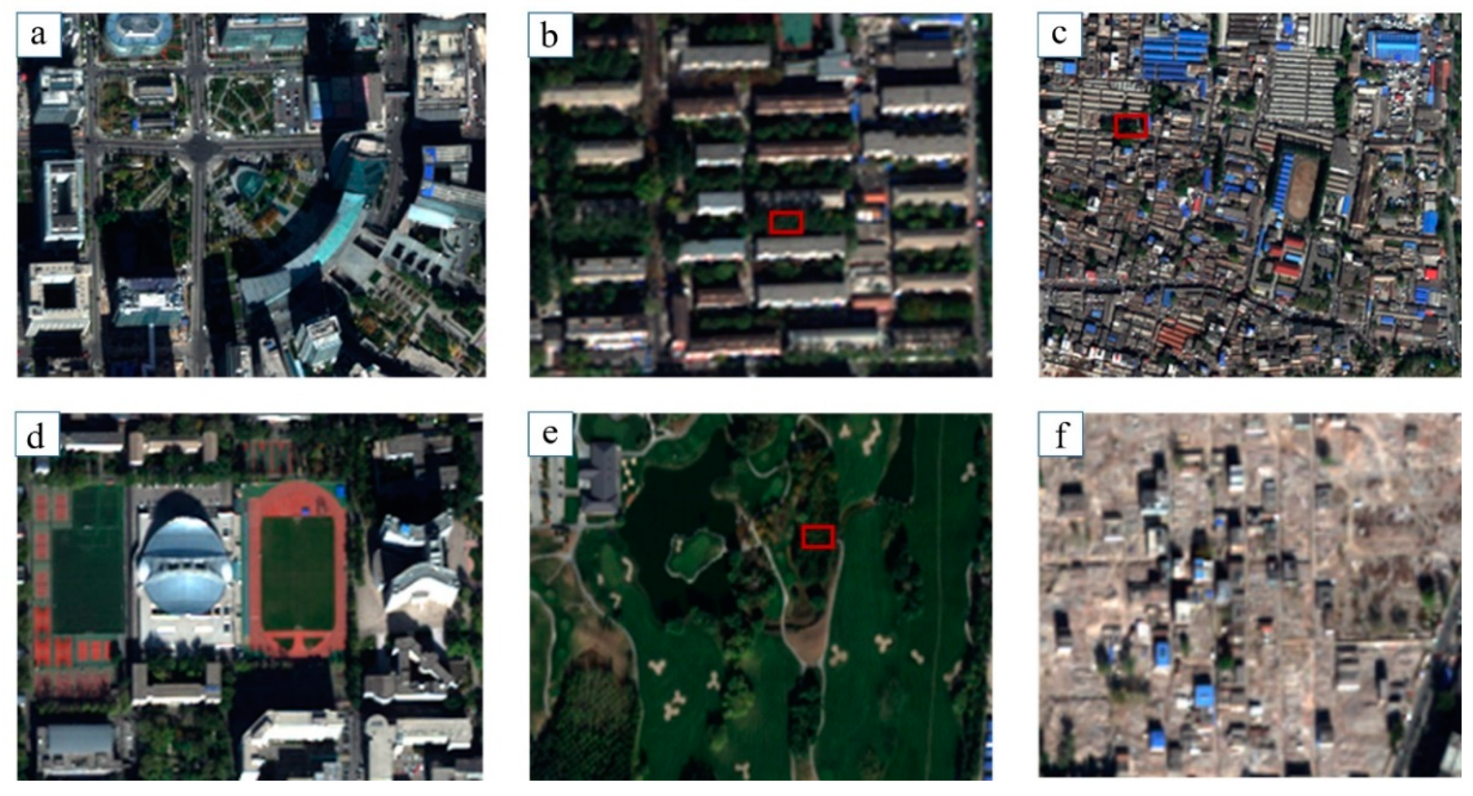
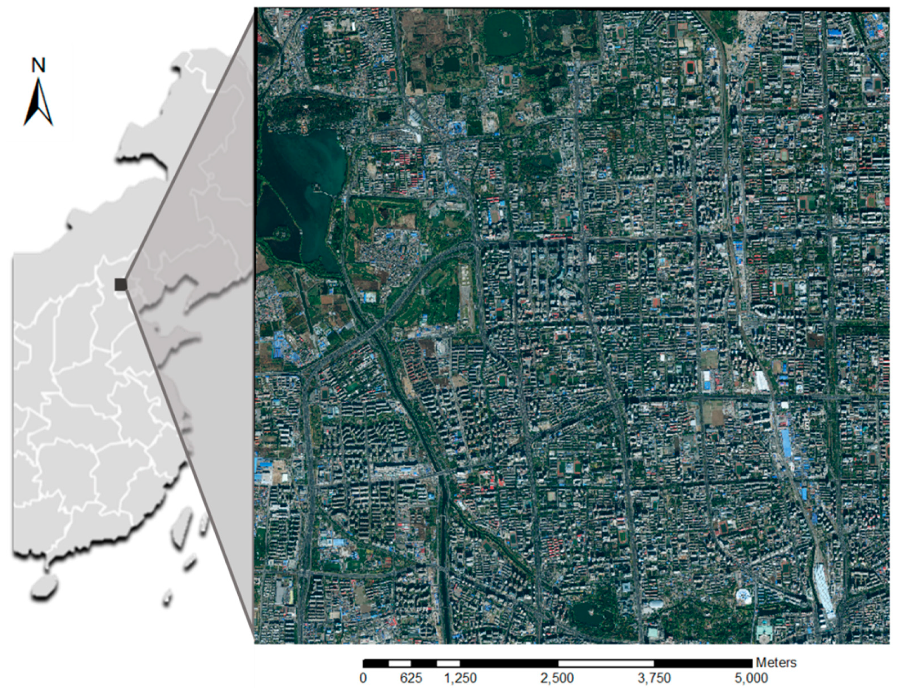
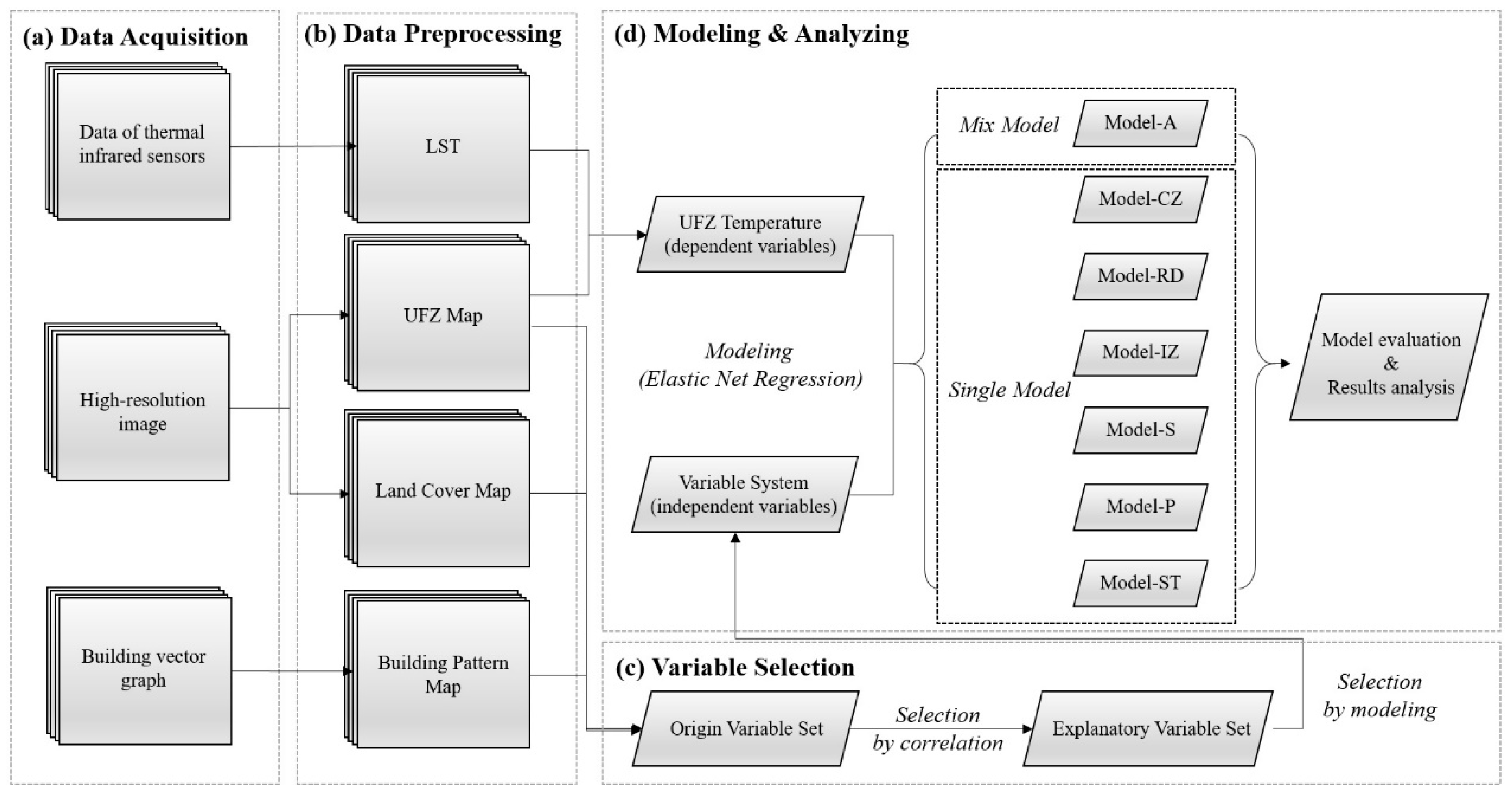
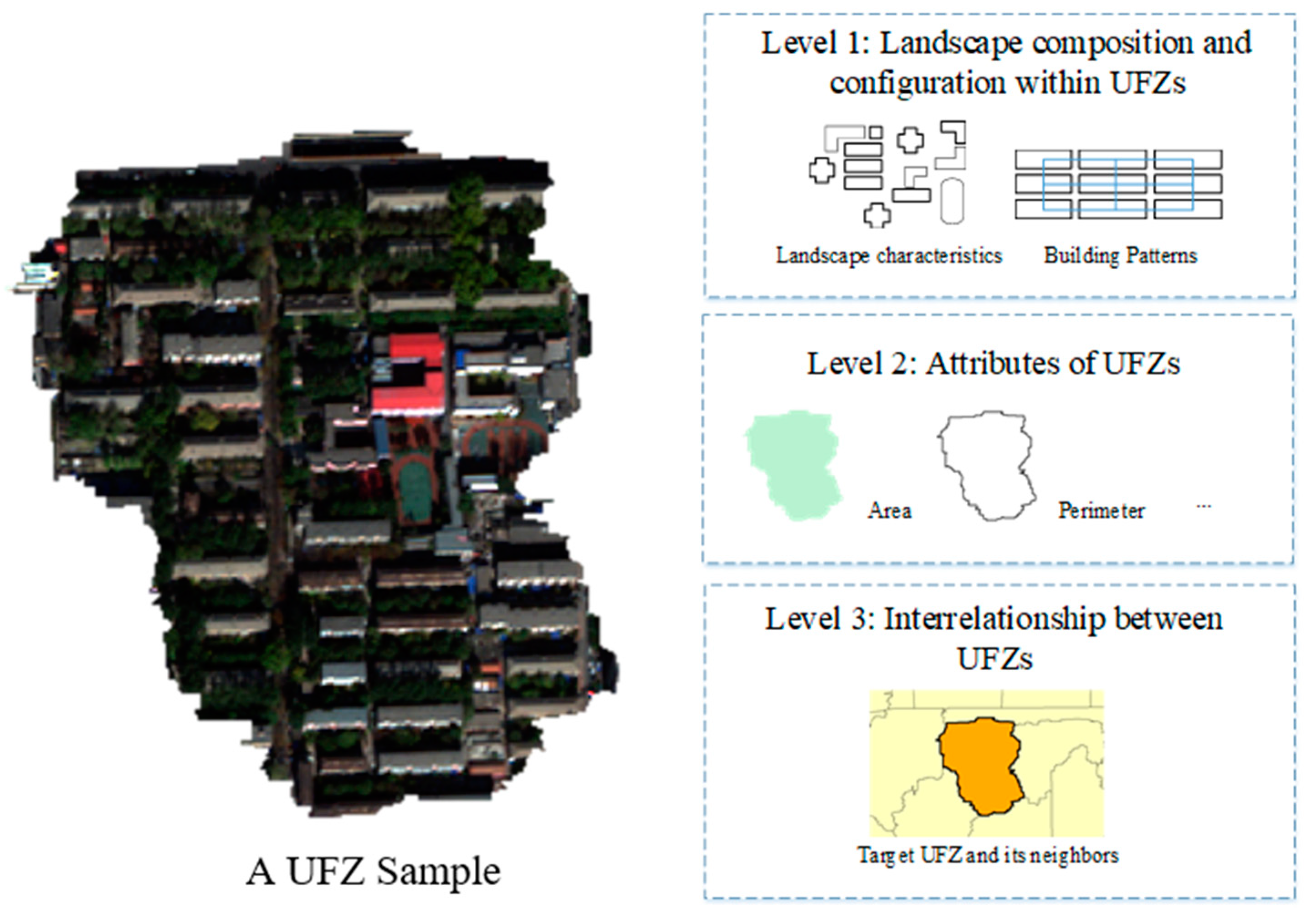
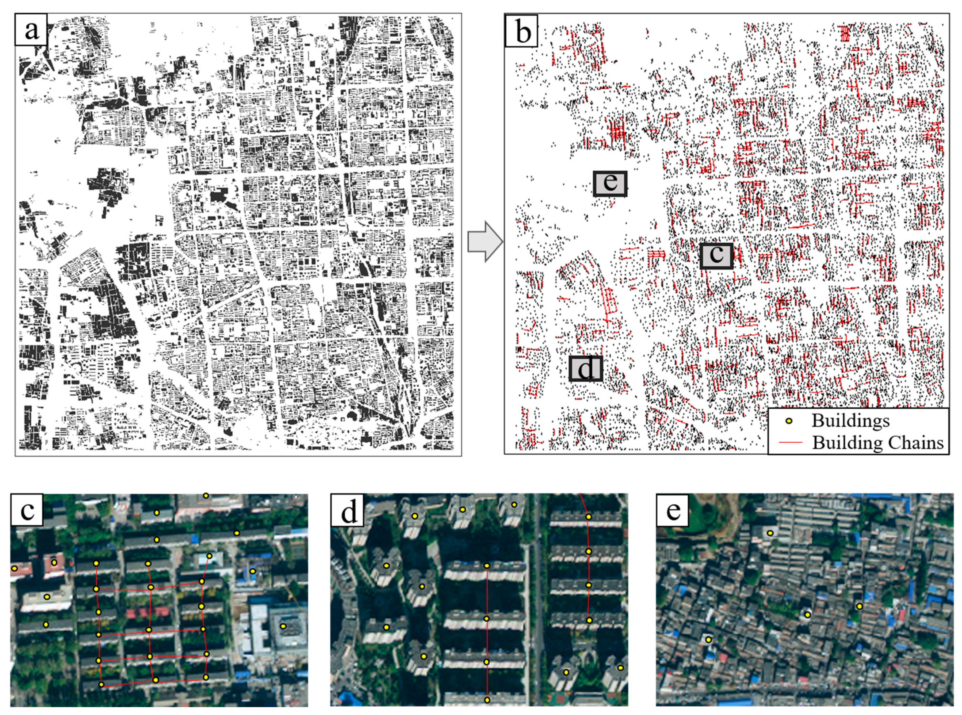
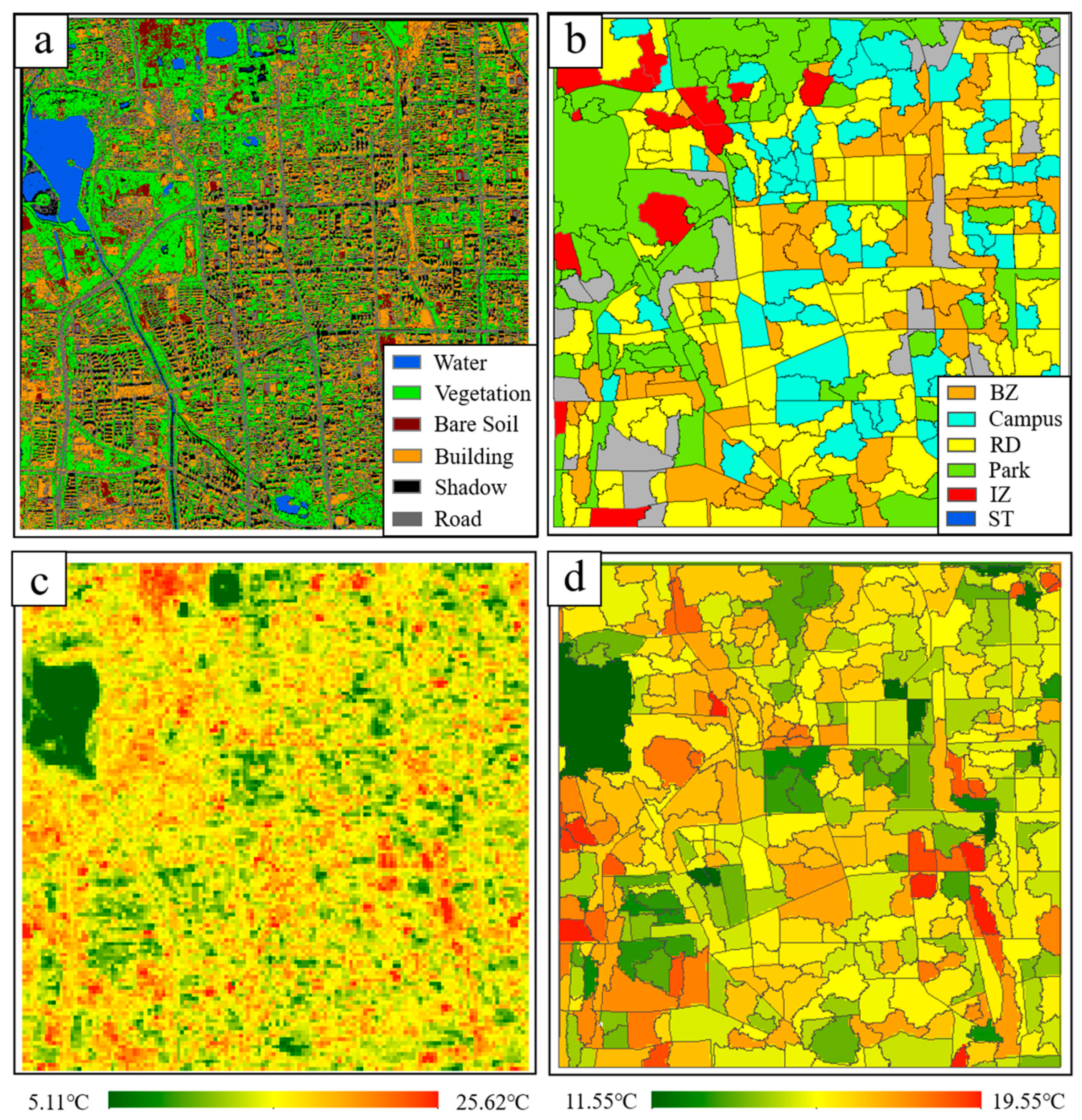
Table 1.
The variables for landscape composition and configuration (Level 1).
| Variables | Definitions |
|---|---|
| PD | The ratio of the number of this feature type of patches to the total; |
| ED | The ratio of the perimeter sum to the area sum of this feature type of patches; |
| IJI | The Interspersion Juxtaposition Index—the observed interspersion over the maximum possible interspersion for the given number of patch types, embodying whether the spatial distribution of adjacencies among unique patch types is even. |
Table 2.
The variables for building patterns (Level 1).
| Variables | Definitions |
|---|---|
| BLD-AREA_SD | The area standard deviation of buildings; |
| NB | The number of buildings; |
| NC | The number of building chains, including the horizontal and vertical direction; |
| LC | The length sum of all the chains |
| RB | The ratio of buildings in chains to the total number of buildings. |
Table 3.
The variables for UFZs at the second level.
| Variables | Definitions |
|---|---|
| Area | The area of the UFZ; |
| Perimeter | The perimeter of the UFZ; |
| SI | Shape Index, the ratio of a UFZ area to the square root of the UFZ perimeter, embodying the complexity of a UFZ’s shape; |
| CONTAG | Contagion Index, embodying the patch types are aggregated or disaggregated; |
| SHDI | Shannon’s Diversity Index, measuring diversity in a UFZ, which is more sensitive to rare patch types than Simpson’s Diversity Index; |
| SIDI | Simpson’s Diversity Index, measuring diversity in a UFZ, which is less sensitive to the presence of rare types. |
Table 4.
The variables for the interrelationship between UFZs at the third level.
| Variables | Definitions |
|---|---|
| Adjacency-CZ | The proportion of the overlapping edge of a UFZ and its neighboring commercial zones; |
| Adjacency-RD | The proportion of the overlapping edge of a UFZ and its neighboring residential districts; |
| Adjacency-IZ | The proportion of the overlapping edge of a UFZ and its neighboring industrial zones; |
| Adjacency-C | The proportion of the overlapping edge of a UFZ and its neighboring campuses; |
| Adjacency-P | The proportion of the overlapping edge of a UFZ and its neighboring parks; |
| Adjacency-ST | The proportion of the overlapping edge of a UFZ and its neighboring shanty towns. |
Table 5.
Definitions of the seven models.
| Model Type | Model Name | Definition |
|---|---|---|
| Single model | Model-CZ | Only commercial zones’ data are used to fit the model aiming to determine the LST–landscape relationships in commercial zones. |
| Model-RD | Only residential zones’ data are used to fit the model aiming to determine the LST–landscape relationships in residential districts. | |
| Model-IZ | Only industrial zones’ data are used to fit the model aiming to determine the LST–landscape relationships in industrial zones. | |
| Model-C | Only campuses’ data are used to fit the model aiming to determine the LST–landscape relationships in campuses. | |
| Model-P | Only parks’ data are used to fit the model aiming to determine the LST–landscape relationships in parks. | |
| Model-ST | Only shanty towns’ data are used to fit the model aiming to determine the LST–landscape relationships in shanty towns. | |
| Mixed model | Model-A | All kinds of UFZs are used to fit the model aiming to determine the uniform LST–landscape relationships in urban areas and to compare them with the other six models. |
Table 6.
The basic information about the valid zones.
| UFZ category | The Num. of zones | Average Area/m2 | The Area Sum/m2 | Average Temperature/℃ |
|---|---|---|---|---|
| Commercial zones | 76 | 154316 | 11728018 | 15.86 |
| Residential Districts | 123 | 179776 | 22112434 | 16.12 |
| Industrial Zones | 13 | 230701 | 2999108 | 17.04 |
| Campuses | 60 | 174149 | 10448926 | 16.64 |
| Parks | 77 | 196955 | 15165552 | 15.70 |
| Shanty Towns | 25 | 182222 | 4555560 | 17.50 |
| Sum | 374 | 179170 | 67009598 | —— |
Table 7.
Model Parameters.
| Model-A | Model-CZ | Model-RD | Model-IZ | Model-C | Model-P | Model-ST | |
|---|---|---|---|---|---|---|---|
| Alpha | 0.2 | 0.9 | 0.1 | 0.2 | 0.4 | 0.3 | 0.4 |
| L1_Ratio | 0.1 | 0.1 | 0.1 | 0.1 | 0.1 | 0.1 | 0.1 |
Table 8.
The goodness of fit of the seven models.
| Model-A | Model-CZ | Model-RD | Model-IZ | Model-C | Model-P | Model-ST | |
|---|---|---|---|---|---|---|---|
| 0.48 | 0.41 | 0.63 | 0.94 | 0.55 | 0.67 | 0.75 |
Table 9.
Spatial autocorrelation of the model residuals.
| Model-A | Model-CZ | Model-RD | Model-IZ | Model-C | Model-P | Model-ST | |
|---|---|---|---|---|---|---|---|
| Moran’s I | 0.11 | 0.24 | 0.11 | −0.04 | 0.00 | 0.23 | −0.13 |
| Z-Value | 3.43 | 2.56 | 2.06 | 0.33 | 0.25 | 1.65 | −0.48 |
| P-Value | 0.01 | 0.01 | 0.04 | 0.74 | 0.80 | 0.10 | 0.63 |
| Model residuals | Clustered | Clustered | Clustered | Random | Random | Random | Random |
Table 10.
The Numbers of influential variables.
| Model-A | Model-CZ | Model-RD | Model-IZ | Model-C | Model-P | Model-ST | |
|---|---|---|---|---|---|---|---|
| Number | 15 | 8 | 20 | 14 | 15 | 17 | 19 |
Table 11.
Model Coefficients 1.
| Model-A | Model-CZ | Model-RD | Model-IZ | Model-C | Model-P | Model-ST | |
|---|---|---|---|---|---|---|---|
| Area | −0.04 | —— | —— | —— | —— | −0.16 | —— |
| Perimeter | 0 | —— | —— | —— | —— | −0.02 | —— |
| SI | 0 | —— | —— | —— | —— | −0.02 | —— |
| CONTAG | 0 | 0 | −0.10 | —— | —— | −0.12 | 0.07 |
| SHDI | —— | −0.04 | —— | −0.05 | —— | —— | −0.03 |
| SIDI | —— | −0.06 | —— | 0 | —— | —— | −0.06 |
| Adjacency-CZ | 0 | 0 | 0.05 | 0.01 | 0 | 0 | 0 |
| Adjacency-RD | 0 | 0 | −0.04 | −0.14 | 0.03 | 0 | 0 |
| Adjacency-IZ | 0 | 0 | −0.03 | 0 | 0.02 | 0.06 | 0.08 |
| Adjacency-C | 0.03 | 0 | 0.06 | 0 | −0.01 | 0 | −0.08 |
| Adjacency-P | 0 | 0 | −0.09 | 0 | 0.03 | −0.09 | 0 |
| Adjacency-ST | 0.04 | 0 | 0.01 | 0.07 | −0.04 | 0.12 | 0.08 |
| Building | |||||||
| BLD-AREA_SD | 0.07 | 0.04 | −0.04 | —— | −0.07 | —— | 0.05 |
| BLD-ED | —— | —— | —— | 0.05 | —— | —— | 0 |
| BLD-IJI | —— | —— | —— | —— | —— | —— | −0.01 |
| BLD-PD | 0.03 | —— | —— | —— | —— | —— | —— |
| BLD-PLAND | 0 | 0 | −0.04 | 0.02 | −0.05 | 0 | 0.01 |
| NB | —— | —— | 0.13 | 0.08 | —— | −0.08 | —— |
| NC | —— | —— | 0.04 | —— | —— | —— | —— |
| LC | —— | —— | 0 | —— | —— | —— | —— |
| RB | —— | —— | 0.01 | —— | —— | —— | —— |
| Vegetation | |||||||
| VEG-ED | —— | —— | 0 | 0 | —— | 0.10 | −0.06 |
| VEG-IJI | −0.07 | −0.04 | −0.15 | −0.03 | —— | —— | −0.1 |
| VEG-PD | —— | —— | —— | —— | —— | 0 | −0.01 |
| VEG-PLAND | 0 | 0 | 0 | 0 | 0 | 0 | 0 |
| Road | |||||||
| Road-ED | —— | 0 | —— | 0.16 | —— | —— | —— |
| Road-IJI | —— | —— | 0.11 | −0.04 | 0.12 | 0.02 | −0.08 |
| Road -PD | −0.03 | —— | —— | —— | −0.06 | —— | —— |
| Road -PLAND | 0.06 | 0 | 0.15 | 0 | 0.07 | 0.04 | 0 |
| Shadow | |||||||
| Shadow-ED | −0.23 | −0.14 | −0.10 | 0 | −0.05 | −0.21 | −0.13 |
| Shadow-IJI | —— | —— | 0.16 | −0.05 | —— | —— | −0.03 |
| Shadow-PD | 0 | −0.03 | —— | −0.07 | 0 | −0.08 | −0.03 |
| Shadow-PLAND | −0.26 | −0.20 | −0.22 | 0 | −0.14 | −0.13 | −0.03 |
| Bare Soil | |||||||
| Bare Soil-ED | 0 | —— | −0.04 | —— | 0.02 | 0 | —— |
| Bare Soil-IJI | —— | —— | 0.05 | —— | 0.07 | —— | −0.03 |
| Bare Soil-PD | 0 | —— | —— | 0.05 | —— | 0 | —— |
| Bare Soil-PLAND | 0.13 | 0.05 | 0 | 0.05 | 0.04 | 0.18 | 0.10 |
| Water | |||||||
| Water-ED | −0.01 | —— | —— | —— | −0.06 | —— | |
| Water-IJI | −0.06 | —— | —— | —— | —— | —— | —— |
| Water-PD | −0.02 | —— | —— | —— | —— | 0 | —— |
| Water-PLAND | −0.15 | —— | —— | —— | —— | −0.18 | —— |
| Interception | 16.33 | 15.94 | 16.06 | 16.95 | 16.70 | 16.37 | 17.51 |
1 Symbol “——” means that the corresponding variable was already excluded in the first round of the variable selection and does not take part in the model fitting. The zero value means the variable plays a limited role in the model and has little effect on the results of modeling. The positive and negative values correspond to the heating and cooling effects on LST, and the magnitude of the value indicates how strong the LST effects the corresponding variable in that model. The interceptions are also provided in Table 11, reflecting the average value of the units in the model, namely the average LST of the involved UFZs.
© 2019 by the authors. Licensee MDPI, Basel, Switzerland. This article is an open access article distributed under the terms and conditions of the Creative Commons Attribution (CC BY) license (http://creativecommons.org/licenses/by/4.0/).
Share and Cite
MDPI and ACS Style
Feng, Y.; Du, S.; Myint, S.W.; Shu, M. Do Urban Functional Zones Affect Land Surface Temperature Differently? A Case Study of Beijing, China. Remote Sens. 2019, 11, 1802. https://0-doi-org.brum.beds.ac.uk/10.3390/rs11151802
AMA Style
Feng Y, Du S, Myint SW, Shu M. Do Urban Functional Zones Affect Land Surface Temperature Differently? A Case Study of Beijing, China. Remote Sensing. 2019; 11(15):1802. https://0-doi-org.brum.beds.ac.uk/10.3390/rs11151802
Chicago/Turabian StyleFeng, Yuning, Shihong Du, Soe W. Myint, and Mi Shu. 2019. "Do Urban Functional Zones Affect Land Surface Temperature Differently? A Case Study of Beijing, China" Remote Sensing 11, no. 15: 1802. https://0-doi-org.brum.beds.ac.uk/10.3390/rs11151802
Note that from the first issue of 2016, this journal uses article numbers instead of page numbers. See further details here.