Detection of Soil Pipes Using Ground Penetrating Radar


1
Institute of Geography and Spatial Management, Faculty of Geography and Geology, Jagiellonian University, ul. Gronostajowa 7, 30-387 Kraków, Poland
2
Department of Applied Geology, Faculty of Earth Sciences, University of Silesia, ul. Będzińska 60, 41-200 Sosnowiec, Poland
*
Author to whom correspondence should be addressed.
Remote Sens. 2019, 11(16), 1864; https://0-doi-org.brum.beds.ac.uk/10.3390/rs11161864
Submission received: 20 June 2019
/
Revised: 22 July 2019
/
Accepted: 2 August 2019
/
Published: 9 August 2019
(This article belongs to the Special Issue Recent Progress in Ground Penetrating Radar Remote Sensing)
Abstract
:Soil piping leads to land degradation in almost all morphoclimatic regions. However, the detection of soil pipes is still a methodological challenge. Therefore, this study aims at testing ground penetrating radar (GPR) to identify soil pipes and to present the complexity of soil pipe networks. The GPR surveys were conducted at three sites in the Bieszczady Mountains (SE Poland), where pipes develop in Cambisols. In total, 36 GPR profiles longitudinal and transverse to piping systems were made and used to provide spatial visualization of pipe networks. Soil pipes were identified as reflection hyperbolas on radargrams, which were verified with the surface indicators of piping, i.e., sagging of the ground and the occurrence of pipe roof collapses. Antennas of 500 MHz and 800 MHz were tested, which made possible the penetration of the subsurface up to 3.2 m and 2 m, respectively. Concerning ground properties, antenna frequencies and processing techniques, there was a potential possibility to detect pipes with a minimum diameter of 3.5 cm (using the antenna of lower frequency), and 2.2 cm (with the antenna of higher frequency). The results have proved that soil pipes meander horizontally and vertically and their networks become more complicated and extensive down the slope. GPR is a useful method to detect soil pipes, although it requires field verification and the proper selection of antenna frequency.
1. Introduction
Soil piping is a widespread land degradation process [1,2] that occurs in different soil types under various climatic and land use conditions [3]. This process leads to the formation of linear tunnels (pipes) by concentrated flowing water in soils [4]. The subsurface network of pipes creates paths for water and sediments affecting slope-channel coupling. Despite its role in sediment and hydrological connectivity, there is still a lack of basic information on the morphological characteristics of pipes and pipe networks and there is a high need to develop methods to detect soil pipes [3].
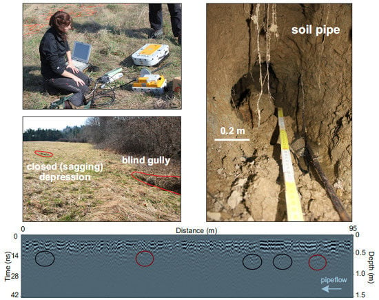
Although soil piping is a subsurface process, it is often investigated through surface indicators, mainly by mapping pipe roof collapses (PCs) [3,5,6] (Figure 1). However, this method cannot provide complete information on the subsurface pipe network, its extension, lateral and vertical changes of a pipe size, length, and tortuosity. The mapping of PCs may lead to the underestimation of network density up to 50%, which was already reported in blanket peats in the Pennine Hills, UK [7] and in mid-altitude mountains in the Carpathians, Poland [8]. So far, research on soil pipes has presented only limited information on their morphometry and morphology, most often providing only a pipe diameter [5,6,9,10], although Terajima et al. [11] found that the morphology of soil pipes can change rapidly over very short distances. Until now, there have been limited detailed studies on soil pipe morphology, and they have mainly focused on forms up to 1 m long in forested hillslopes [11,12]. There has been no such research in grassland and pastures, where soil pipes may reach several meters long, e.g., in loess-covered hills or mountainous regions.
Geophysical methods seem to be a promising tool to provide new, more detailed information on subsurface pipes. In natural environments, the following methods have already been tested in soil piping research: electrical resistivity tomography (ERT) [8,13,14,15], seismic refraction tomography (SRT) [16], self-potential (SP) [17], and ground penetrating radar (GPR) [7,8,18,19,20,21,22]. Under laboratory conditions, active and passive acoustic techniques have been tested to study pipe flow and internal erosion [23]. Among these methods, GPR has received the most attention, even though it seems that the potential of this method has not yet been fully exploited. Most reports have presented the preliminary results of GPR application in the detection of soil pipes [7,8,20], including only short conference abstracts [18,19]. On one occasion GPR was used to establish hydrological connectivity between pipes through the use of a tracer solution [21] and to estimate the pipe length [8]. Antennas of different frequencies were used, e.g., in the northern Pennine Hills (UK)—100 and 200 MHz [7,21], in the Bieszczady Mountains (Poland)—500 MHz, and in the loess belt in Belgium (Sippenaeken and Kluisbergen)—200 and 400 MHz [18,19].
The main aim of this study is to detect soil pipes using GPR in order to better understand the complexity of a pipe network. The detailed objectives are:
- to identify the lateral and vertical changes of soil pipes,
- to present spatial visualization of GPR profiles, which provides possible distribution and characteristics of soil pipe networks,
- to assess the suitability of GPR application for soil pipe detection.
The study is based on the examples found in a mountainous area under a temperate climate, where soil pipes develop in Cambisols. The study sites (the Cisowiec and Bereźnica catchments) have been already identified as piping-prone areas [5]. Moreover, the study sites in the Bereźnica catchment have been already explored [8] using GPR and ERT in order to assess the usefulness of these geophysical methods in silty-clayey materials which occur there. As this preliminary study [8] proved that GPR can be used in soil pipe detection, the present study aims to provide more detailed information on the complexity of a pipe network. The novelty of the present study lies in the spatial visualization of soil pipe networks that expands knowledge on the lateral and vertical changes of soil pipes. Additionally, the new site in the Cisowiec catchment has been studied using different antenna frequency, which enables discussion on the methodological aspect of the use of GPR in soil pipe detection. The results of study have revealed the complex morphology of soil pipe networks underlying the fact that one main pipe is often associated with smaller pipes, as well as the fact that all the pipes meander in two dimensions—horizontally and vertically. Moreover, this study has emphasized the critical key in GPR surveys of soil piping, i.e., the selection of antennas with appropriate frequency which allowing the identification of pipes of different sizes and depths of development. Knowledge of the soil pipe network is crucial for a better understanding of hillslope hydrology, and soil erosion by piping.
2. Materials and Methods
2.1. Study Area
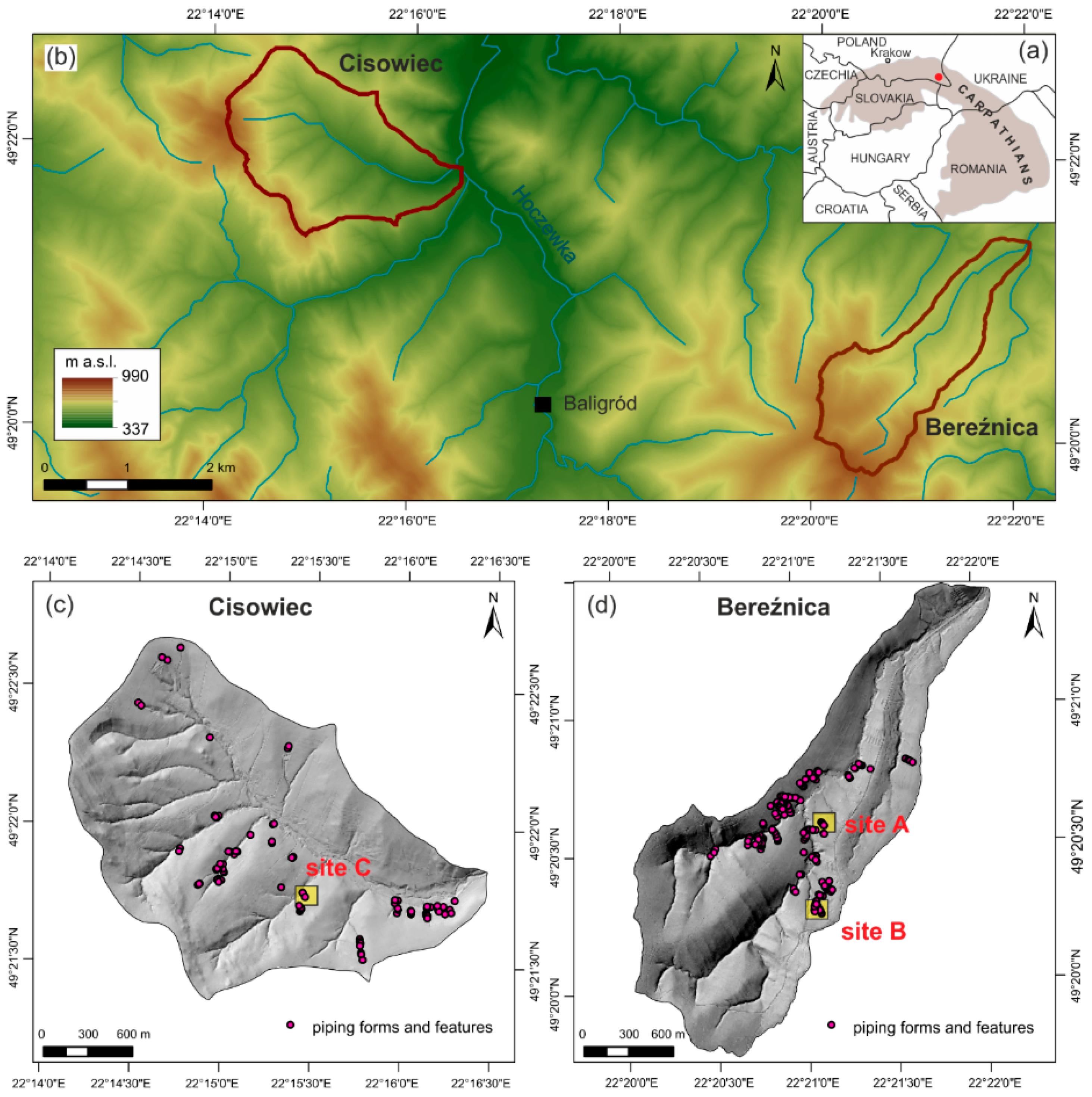
The study was conducted in two catchments: (1) the Bereźnica (305 ha) and (2) the Cisowiec catchment (388 ha), where three sites were selected for the detailed geophysical survey (Figure 2). The catchments are located in the south-eastern part of Poland in the Bieszczady Mountains, which are part of the Outer Eastern Carpathians. They represent mid-altitude mountains with altitudes ranging from 502 to 748 m above sea level (a.s.l.) in Bereźnica, and from 400 to 742 m a.s.l. in Cisowiec. The lithology consists of folded Tertiary flysch facies, i.e., thick-bedded sandstones alternating with shales and mudstones. The parallel ridges oriented northwest to southeast are developed on resistant sandstones (the Krosno and Cisna Formations), whereas the valleys are carved into less resistant shales and mudstones [24]. The mean slope gradient is 12° in Bereźnica and 15° in Cisowiec. The parent material for soils is slope deposits derived from the weathering of flysch rocks with an aeolian admixture [25]. In the study area, mainly Cambisols occur [26], and in places with high soil moisture content, Gleysols developed.
Both catchments are covered by grasslands and the south and south-western part of them are covered by mixed coniferous forests with a predominance of beech, and occasionally associated with spruce. The climate is humid continental (according to the Köppen–Geiger climate classification) with a mean annual temperature of 7.0 °C and a mean annual precipitation of 900 mm (according to data obtained from the Institute of Meteorology and Water Management—State Research Institute, IMGW-PIB, in Poland for the years 1960–2015 recorded at the Baligród–Mchawa and Terka weather stations).
The Bieszczady Mountains were already reported as a piping-prone region [5]. It has been stated that the combination of biological activity and soil properties (silty texture, well-developed soil structure, low bulk density, and high porosity) favour pipe development [26]. Soil pipes develop at the soil-bedrock interface [26]. In the study areas, the mean depth of pipe development is 0.8 m with a maximum of 1.6 m.
2.2. Field Data Collection
2.2.1. Geomorphological Mapping
In order to explore soil piping in the study areas and to choose the study sites with piping systems for geophysical survey (Figure 2), detailed geomorphological mapping was performed. The surface indicators of piping erosion were identified based on the classification presented by Bernatek-Jakiel and Poesen [3]. The following piping-related forms were mapped: closed (sagging) depressions, sinkholes, and blind gullies (Figure 1). All the forms were recorded using a hand-held global positioning system (GPS) receiver with accuracy <3 m (Garmin GPSMap 62s), as well as their dimensions (length, width and depth) were measured using a measuring tape.
The digital elevation model (DEM) of the catchments is based on aerial LiDAR (Light Detection and Ranging) scanning performed with an accuracy of 4 points per 1 m2 obtained from the Head Office of Geodesy and Cartography in Poland (GUGiK). The detailed DEM of the study sites (sites A and B) in the Bereźnica catchment selected to the geophysical research is based on the manual geodetic measurements using an electronic total station (Topcon Hiper II) with an accuracy of 0.2 m, whereas the detailed DEM of the study site (site C) in the Cisowiec catchment is based on SfM (Structure-from-Motion) photogrammetry. An unmanned aerial vehicle (UAV), DJI Phantom-4 equipped with a 1’ camera was used to acquire aerial photographs. In order to achieve high resolution, the flying height was set at 10–15 m above the ground and 684 photos were taken. The flight survey was conducted in spring (March 2019) at noon in a good weather in order to reduce shadow effects. The orthoimage mosaic and DEM of 0.5 cm/pixel resolution were generated through the SfM photogrammetry using Agisoft Photoscan software.
2.2.2. Ground-Penetrating Radar Survey
GPR is a non-destructive and non-invasive method based on high-frequency (usually from 1 MHz to 1000 MHz) electromagnetic wave propagation [27]. It detects electrical discontinuities in a shallow subsurface. The GPR system consists of transmitter and receiver antennas. The transmitter antenna propagates electromagnetic pulses through the subsurface, which are then reflected depending on the electromagnetic properties of the ground. The penetration depth and resolution of radargrams depend on the electromagnetic properties of the materials, and on the frequency of the antenna being used. The details of theory that underlies the GPR method is already presented in the literature [28,29].
GPR measurements were carried out at three study sites (Figure 2). In total, 36 GPR profiles were performed (Figure 3), including 8 profiles longitudinal and 27 transverse to the piping systems (Table 1). In site C, one additional GPR profile that followed surface indicators of a piping system was performed. In sites A and B, profiles were obtained mainly transversely to the piping systems, whereas in site C more longitudinal profiles were done as the piping system runs more diagonally on a hillslope.
The RAMAC GPR system (Malå GeoScience) with 500 MHz and 800 MHz shielded antennas with a GPS receiver (Leica) was used in the study. The use of antennas of different frequencies was motivated by the need to compare their usefulness in soil pipe detection. RAMAC GroundVision software (Malå GeoScience) was used for operating the radar and the initial processing of the data: data acquisition, filtering, and marking the pipes visible on the surface. The time windows of data collection were selected as 61 ns and 100 ns, respectively for Bereźnica and Cisowiec. Sampling frequency was set as 10 times the antenna frequency and the number of samples was set to the value of 500 for both catchments, which made possible the best performance of the measurements. Obtained radargrams were processed and interpreted in the RadExplorer software (DECO Geophysical Ltd.). Basic processing steps were applied to the raw data and included trace editing, filtering, and data correction. Data editing involved reorganization of the data, i.e., some of the traces needed to be reversed or omitted to obtain a good standard of the interpretation. Direct current removal was used to subtract each trace and remove the offset. The time for the first arrival was set to be zero using Zero Time Adjustment function. Background removal and amplitude correction were used to make smaller structures more visible. Bandpass filtering was also used letting through frequencies either side of the peak frequency of the transmitted signal. After signal processing, the velocity models were based on a dielectric constant and electromagnetic wave propagation velocity of ε = 18 and v = 7.1 cm ns−1, respectively. These values are characteristic for clayey soils with high concentration of water and an electrical conductivity of 500 mS m−1 [30]. The selection of ε and v values was based on the known depth of the detected pipes in the field, allowing time to depth conversion. The obtained depth recognition is presented in Table 1.
The soil pipes were filled with air, and in the bottom the increased soil moisture and water were present. These subsurface tunnels are reflected on radargrams as reflection hyperbolas when they are crossed transversely, as singular strong reflections [18], or as an anomaly in the reflections [8]. All reflections that might potentially suggest pipe occurrence were interpreted in their relation to others within a profile, or between two consecutive profiles and they were related to the surface indicators of piping (i.e., sagging of the ground or pipe roof collapses). Once the processing was completed, reflections and hyperbolas were detected manually.
3. Results
3.1. The Bereźnica Catchment
In the Bereźnica catchment, 179 piping forms were mapped (Figure 2d), including 61 closed (sagging) depressions, 96 sinkholes, and 22 blind (discontinuous) gullies. Additionally, 32 piping-related features (2 pipe inlets and 30 pipe outlets) were identified. All these forms are grouped in 38 piping systems (B1 to B38). The closed (sagging) depressions are characterized by a mean length of 3.3 m, a mean width of 1.3 m, and a mean depth of 0.4 m. The sinkholes have a mean length of 0.7 m, a mean width of 0.6 m, and a mean depth of 0.8 m, whereas the blind (discontinuous) gullies are on average 5.1 m long, 1.8 m wide, and 0.9 m deep. More details have already been published [8].
3.1.1. Site A
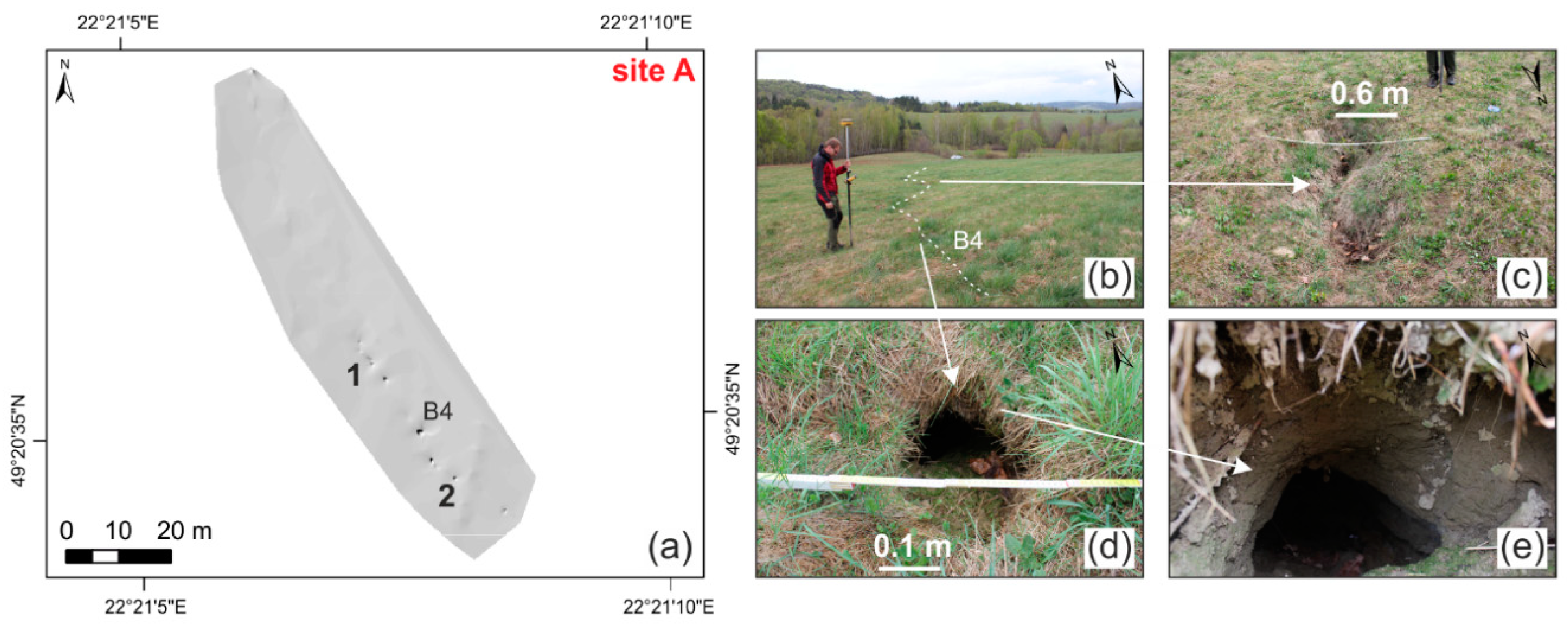
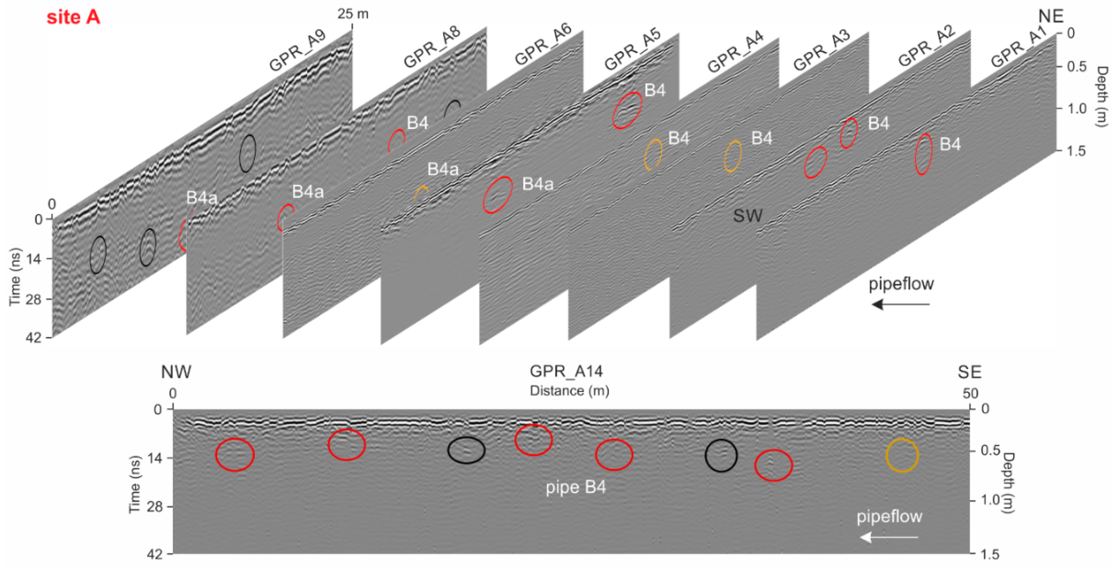
Site A is located in the central part of the Bereźnica catchment (Figure 2d) on a hillslope covered by grasslands. The hillslope is exposed to the NW and the slope gradient is 8–10°. Piping system B4 consists of three closed (sagging) depressions and six sinkholes. The mean depth of a pipe development is between 0.7 m and 0.8 m. The length of this system is 44.4 m (measured from the most upslope, through the next, to the lowermost piping form). Figure 4 presents the surface indicators of soil piping in site A.
Soil pipes are reflected on radargrams as hyperbolas (Figure 5), when they are scanned transversely, otherwise pipes may be marked as just an anomaly in reflection (e.g., GPR_A14, Figure 5). The main pipe B4, which is visible at the surface through several pipe collapses (Figure 4), is reflected relatively well on radargrams. Near this pipe, there is potentially a pipe B4a which may constitute a new separate pipe or a pipe that connects with the main pipe B4. This pipe is quite well reflected on radargrams, but the surface in this area is just slightly sagging, without any clear pipe collapse which would exhibit the subsurface pipe. Reflections of pipes on radargrams are noted at different depths (see GPR_A14, Figure 5) and their horizontal course is not straightforward along slope inclination. This indicates that pipes meander both vertically and horizontally.
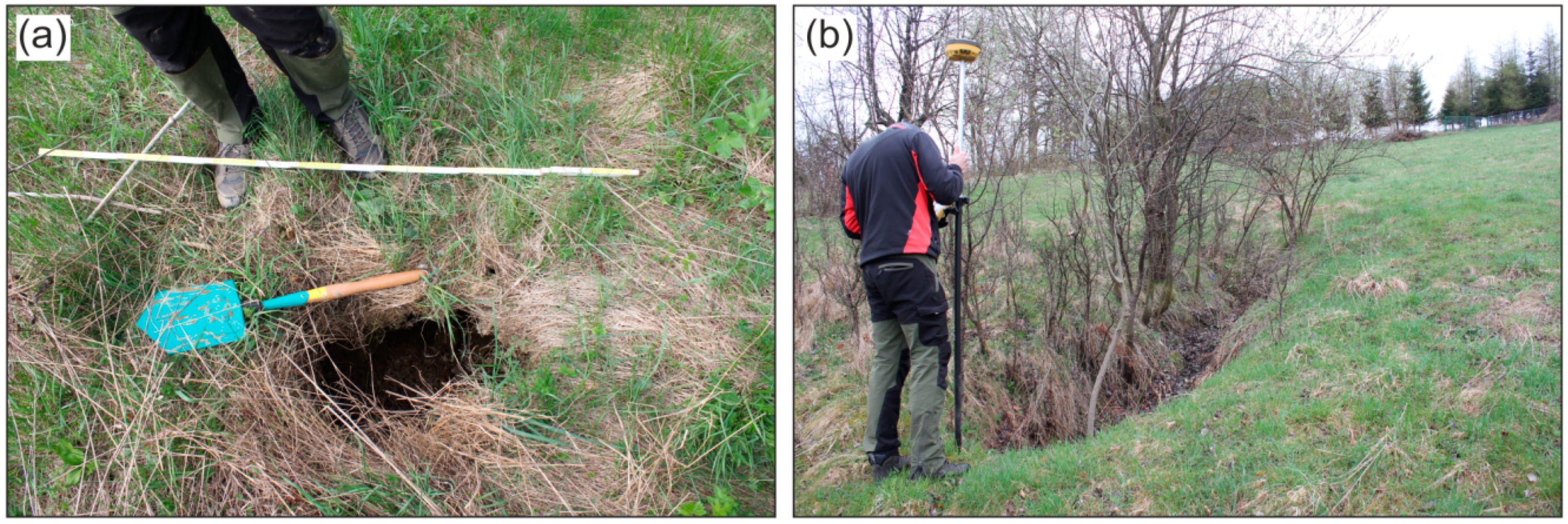
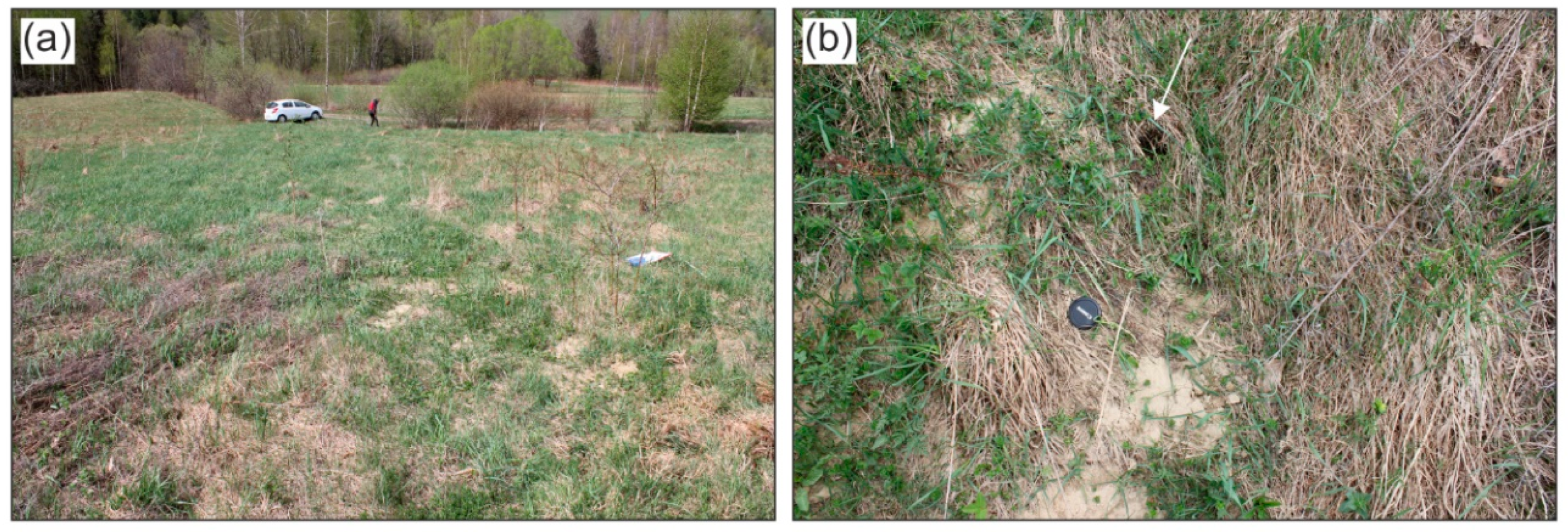
Moreover, there are very clear reflections on radargrams below the piping systems B4 and B4a that suggest the existence of pipes, but there are no clear surface indicators. These may indicate the end of these pipes (B4 and B4a) which may be clogged (there are no reflections on consecutive lower-situated radargrams GPR_A11-GPR_A13, see Figure 3). Interestingly, there is a zone with very fine-grained materials that lie on the surface. This may be the materials washed out from the pipes (Figure 6). However, just one possible pipe outlet was seen in the field (Figure 6b), others were probably clogged and obscured with materials and vegetation.
3.1.2. Site B
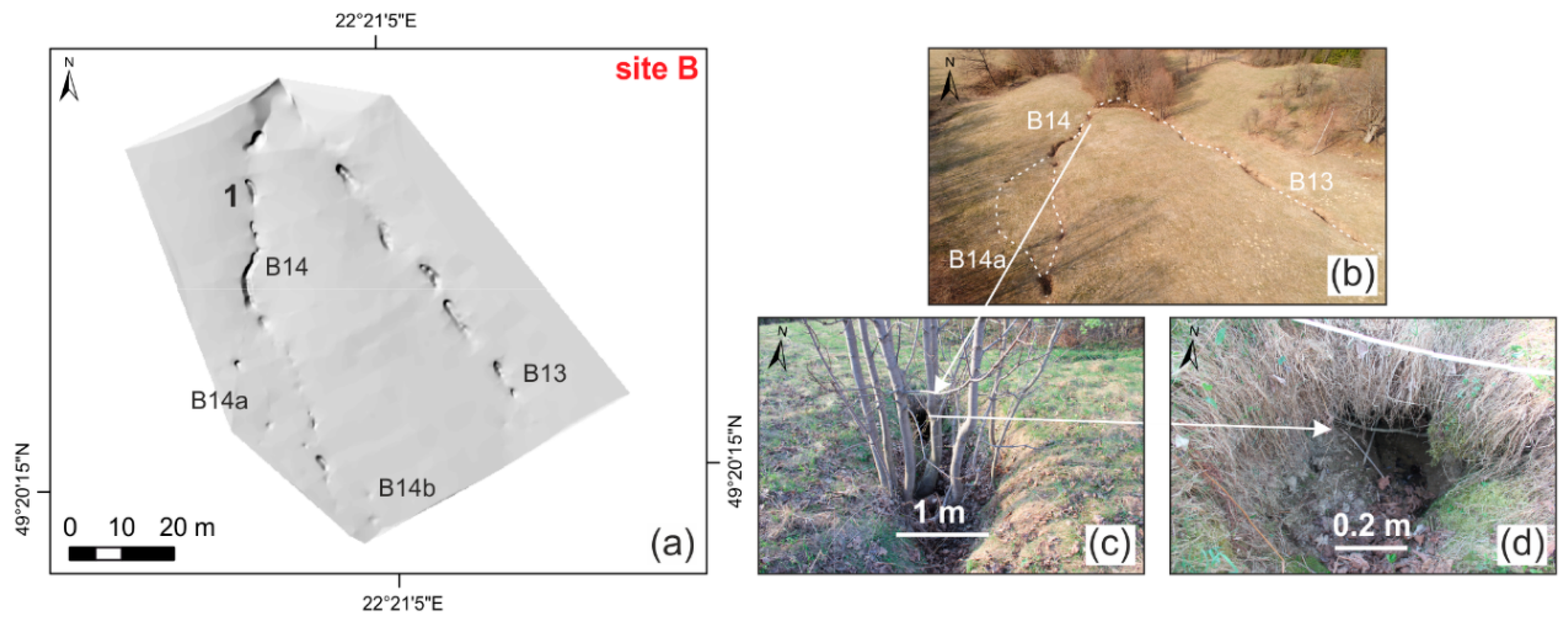
Site B is located in the central part of the Bereźnica catchment (Figure 2d) on a hillslope exposed to the NW, and with a slope gradient of 10–15°. Piping systems B13 and B14 are located in grassland and they end at pipe outlets in the gully head covered by the forest. System B13 consists of four closed (sagging) depressions, three sinkholes, and two blind (discontinuous) gullies. The length of system B13 is 74.7 m (measured from most upslope, through the next, to the outlet), and the pipe develops at a depth of 0.7–1.55 m. System B14 consists of eight closed (sagging) depressions, seven sinkholes, and three blind gullies. The depths of the pipes ranges from 0.65–1.60 m. Previous studies revealed that system B14 consists of one main pipe (B14) and probably two shorter pipes (B14a and B14b) combined with the main one [8]. The whole length of this system is 140.7 m (measured from the most upslope, through the next, to the outlet). Figure 7 presents the surface indicators of soil piping in site B.
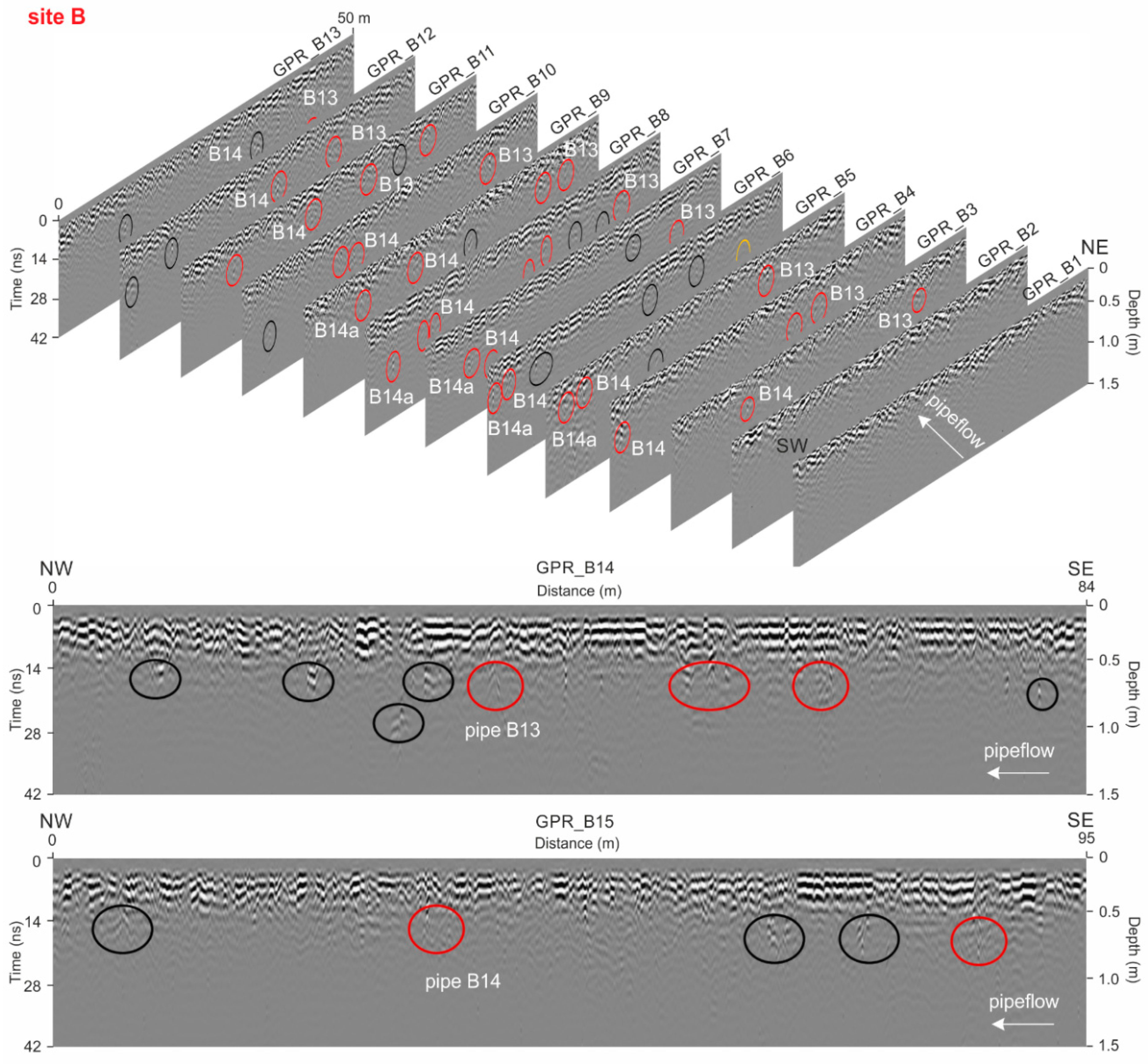
The soil pipes in site B are reflected on radargrams as hyperbolas. In some places, only anomalies in reflection indicate the potential occurrence of soil pipes (Figure 8). This happens when the pipes are not scanned ideally transversely by GPR. The main pipes B13 an B14, which are visible at the surface through several pipe collapses (Figure 7), are well visible on radargrams (Figure 8). Interestingly, just near them other pipes can be noted. In fact, in the field we can sometimes observe two or more pipes that are close to each other and possibly interconnect further in the ground (Figure 9a); in the gully head we also observe several pipe outlets in the place where the main pipe B13 ends (Figure 9b). This is also clearly visible on longitudinal profiles GPR_B14 and GPR_B15 (Figure 8). This suggests that the piping system consists of one main pipe and additional smaller pipes that interconnect with each other. Moreover, as in site A, reflections of pipes on radargrams are noted at different depths (Figure 8) and their horizontal course is not straightforward along the slope inclination, which is also confirmed by the pipe collapses (Figure 7a,b). This means that pipes meander both vertically and horizontally.
There are some places (marked by black circles) where are clear reflections on radargrams, but there are no surface indicators (Figure 8). These reflections occur at profiles GPR_B5 up to GPR_B13. This suggests that downslope potentially new soil pipes are developing, but they are not yet sufficiently large to cause collapses.
3.2. The Cisowiec Catchment
In the Cisowiec catchment, 86 piping forms were mapped (Figure 2c), including 19 closed (sagging) depressions, 51 sinkholes, and 16 blind (discontinuous) gullies. Additionally, 34 piping-related features (3 pipe inlets, 31 pipe outlets) were identified. All these forms are grouped in 34 piping systems (C1 to C34). The closed (sagging) depressions are characterized by a mean length of 2.5 m, a mean width of 1.3 m, and a mean depth of 0.4 m. The sinkholes have a mean length of 0.6 m, a mean width of 0.5 m, and a mean depth of 0.7 m, whereas the blind (discontinuous) gullies are on average 4 m long, 1.5 m wide, and 0.8 m deep.
3.2.1. Site C
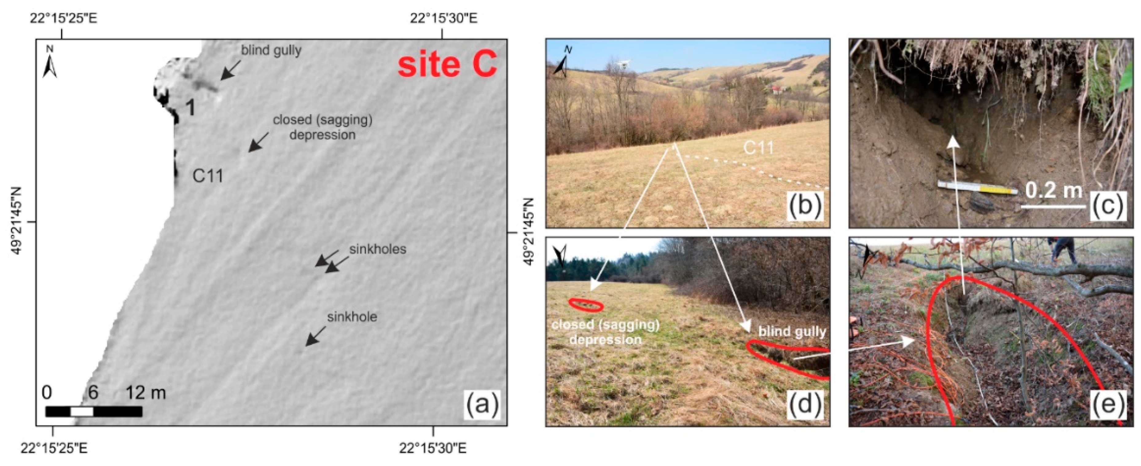
Site C is located in the SEE part of the catchment (Figure 2c) on a hillslope exposed to NW and slope gradient is 9–11°. Piping system C11 is located in grassland and it ends at a pipe outlet in the forest. It consists of two closed (sagging) depressions, three sinkholes, and one blind gully. The length of this system is 44 m (measured from the most upslope, through the next, to the outlet). The pipe develops at a depth of 0.7–0.8 m. Figure 10 presents the surface indicators of soil piping in site C and Video S1 presents the pipe outlet seen in the blind gully (Figure 10c).
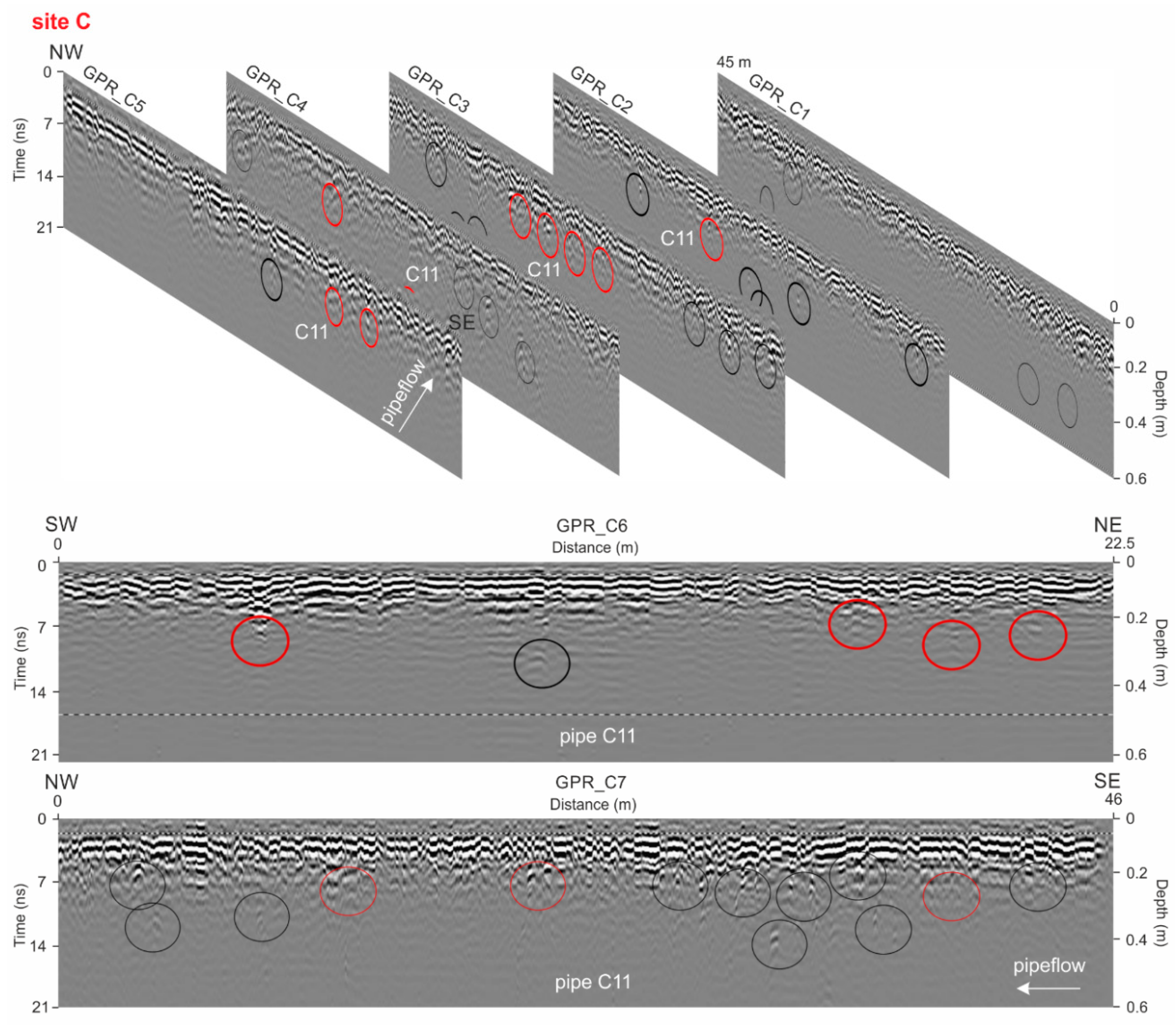
As opposed to sites A and B, the spatial visualization of soil pipe network of site C is based on longitudinal radargrams (Figure 11). The course of pipe C11 is diagonal in relation to the contours, so we had expected better reflections on longitudinal radargrams. Indeed, the hyperbolas are well reflected on radargrams indicating main pipe C11 and additional smaller pipes in the surroundings. The reflection on radargram GPR_C5 indicates clearly the main pipe C11 which is the biggest in this system. Moreover, as at sites A and B, the reflections of the pipes on radargrams are noted at different depths (Figure 11) and their horizontal course, confirmed by the pipe collapses (Figure 10a), is not straightforward. This means that pipes meander both vertically and horizontally.
4. Discussion
4.1. Complexity of the Soil Pipe Network
The detection of PCs does not enable the identification and characterization of a complete underground pipe network. However, the geomorphological role of this subsurface soil erosion process is mainly studied through the surface indicators, i.e., PCs [3,6,8]. For instance, the soil loss is estimated based on the volume of PCs [2,31]. Sometimes the volume of pipes is added to these estimations, but with the assumption that the cross-section of pipes may vary along the longitudinal profile [32] as well as it changes over time because of the dynamics of internal erosion inside the pipe [31,33]. However, the complexity of a pipe network in a vertical and horizontal plan is usually overlooked [1] This indicates that calculations made so far are probably underestimated. This study at three sites (A, B, and C) has confirmed that soil pipes create complex systems that are not fully visible on the surface (Figure 5, Figure 8 and Figure 11). This is especially important in the context of climate change. There is no study on the impact of climate change on piping, although it may be assumed that it can work similarly to gully erosion as these two processes are interrelated [34,35]. Soil loss due to gully erosion is highly sensitive to climate change, and gully head retreat rates, as projected, may increase with 27 to 300% when the precipitation intensities increase [36,37]. This implies that soil loss and gully head retreat due to piping may also increase when the precipitation intensity increases and the scale of this loss may be even larger than we expect.
In 2000, Terajima et al. [11], through the use of a fiberscope, found that pipe morphologies can change rapidly over very short distances. Their results revealed that pipes are almost straight and they run parallel with the slope inclination. However, they studied short pipes generally up to 1 m long on steep forested slopes on Hokkaido, Japan. In this study, pipes from 40 m to more than 140 m long on moderate slopes covered by grasslands were analysed. This study concentrated on the horizontal and vertical changes in pipe position. The horizontal tortuosity has been already proved in the Bieszczady Mountains [8] and it is also confirmed by this study. This is clearly visible not only by the location of PCs which developed, not along a straight line in accordance to the slope inclination (Figure 4a,b, Figure 7a,b and Figure 10a,b), but also on spatial visualizations of the subsurface made by GPR (Figure 5, Figure 8 and Figure 11). The reflection hyperbolas are noted in different positions along the slope. Similarly, the vertical complexity of pipes is indicated both by surface indicators and by the reflection hyperbolas on radargrams. The former is confirmed by the different depths of sinkholes at all sites (A—0.7 m to 0.8 m, B—system B13 from 0.7 m to 1.55 m and B14 from 0.65 m to 1.2 m, C—from 0.7 m to 0.8 m). The latter is confirmed by the reflection hyperbolas which are seen at different depths on radargrams (Figure 5, Figure 8 and Figure 11). This is in contrast to the study of short pipes presented by Terajima et al. [11], which can be attributed to the length and size of pipes, i.e., the longer and the larger pipes, the greater the diversity and complexity. Moreover, the radargrams have confirmed that one main pipe is often associated with two or more pipes that are close to each other and which are possibly interconnected. Sometimes such a situation is visible in the field (Figure 9). This additionally underlines the complexity of soil pipe networks.
The spatial visualizations of soil pipes based on radargrams have revealed that soil pipe networks become more complicated and complex down the slope. This is especially well visible in site B (Figure 8), where more pipes are reflected on radargrams downslope. There are more forms and they are bigger. This is also visible in site C, when we compare profiles GPR_C5 and GPR_C3 (Figure 11). It suggests that energy concentrates down the slope. As it was recently proved [1,34], piping systems in the Bieszczady Mountains develop mainly by elongation up the slope, i.e., PCs firstly occurred in the lower part of the slope, where pipes are bigger, and afterwards, new pipe roof collapses develop up the slope. An interesting situation occurs in site A (Figure 4 and Figure 5), where pipes are probably clogged and the transported materials are washed out on the surface (Figure 6). This may happen owing to the local changes in soil structure and the arrangements of soil horizons (the impermeable layer may be oriented opposite to the slope surface forcing the pipe flow upwards) or just because of the conditions of pipe flow and the characteristics of transported material (e.g., the content of coarse fractions).
4.2. Suitability of GPR Application for Soil Pipe Detection
This study in a complex way has confirmed that GPR can be used to detect soil pipes: this is in accordance with previous reports [7,18,19,20,21]. The reflections on radargrams that indicate soil pipes are well visible because there are significant differences in radar-wave response given by pipes filled with air and with water at the bottom (Figure 4e, Figure 7d and Figure 10c), and with the surrounding soil. Soil pipes are well reflected both on transverse (Figure 5 and Figure 8) and longitudinal (Figure 11) profiles. They meander, so it is almost impossible to scan them always perpendicularly. It seems that the decision on the way of scanning (transversely or longitudinally) is not the most important one. Interestingly, soil pipes are also well reflected when they are scanned along their length, i.e., when the GPR track follows surface indicators of a piping system (profile GPR_C7, Figure 11).
It seems that one of the most crucial things in GPR surveys of soil pipes is the selection of antenna frequencies. Antennas of lower frequencies give deeper penetration, but result in a decrease in resolution; conversely antennas of higher frequencies give higher resolution, but lower depth penetration [38]. In the case of pipes, antennas of high frequencies allow the detailed exploration of pipes which are often characterized by complex morphology (see Section 4.1). On the assumption that the required spatial resolution is approximately 25% of the target depth, suitable frequencies for different exploration depths were proposed [27]. The target depth for pipes is 0.7–0.8 m (with the maximum of 1.6 m) in the Bieszczady Mountains (Poland), so it was proposed to use antennas of 500 to 1000 MHz, and such antennas were used in this study. Moreover, this study was preceded by the detailed geomorphological mapping of PCs in both catchments, as well as by soil studies. Earlier recognition of the areas supported by a theoretical basis was necessary for proper selection of GPR antennas (i.e., their frequencies). The antenna of 500 MHz made it possible to penetrate the subsurface to a greater depth (3.2 m in Bereźnica) in comparison to the antenna of 800 MHz, which achieved a depth of 2 m in Cisowiec (Table 1).
The compromise in the selection of antenna frequencies lies not only in the penetration depth, but also in the resolution. A higher frequency antenna makes it possible to recognize smaller forms as its resolution is better. High electrical conductivity of clayey soils (the content of clay in the soils in Bereźnica is 20–45% and in Cisowiec—15–40%) and high water content (from 30% to almost 60%) cause high attenuation of waves resulting in lower penetration depth, but the resolution may be satisfactory. This happens because wave velocity (v) and wavelength (λ) are lower in materials with high conductivity, leading to an increase in resolution [39]. Radar signal wavelength is a function of antenna frequency (f) and the wave velocity of the signal [40], and as such it was calculated using an equation:
λ = v/f
The resolution was assumed to be one quarter of the GPR wavelength [29,39] and was calculated for the soils which are prone to soil piping. The possible resolution in GPR surveys using antennas of frequencies 100–800 MHz is presented in Table 2. The values of the theoretical resolution can be useful in planning and preparing GPR surveys in different environments. In the Bereźnica catchment, the smallest diameter of a pipe that could be potentially detected using GPR was 3.5 cm, whereas in the Cisowiec catchment it was potentially 2.2 cm (assuming wet clayey soils), considering the frequency of antennas and processing technique used in the study.
The spatial visualization of soil pipe network based on radargrams allowed us to present the horizontal and vertical complexity of pipes (see Section 4.1, Figure 5, Figure 8 and Figure 11). The reflection hyperbolas on radargrams were correlated with surface topography and the occurrence of PCs. However, in some places only the hyperbolas were seen and there was no sagging of the ground above, e.g., no ground sagging above pipe B4 on profile GPR_A9 (Figure 5), the same above pipe B14 on profile GPR_B13 (Figure 8). This indicates that the ground has not subsided yet. This also suggests that the interpretation of radargrams should be always done in relation to the consecutive profiles, but mainly to the surface topography or with trenching [41]. It is only the physical-based proof (here the exposure of soil pipes to the surface as PCs) that may confirm the interpretation of radargrams.
It also happens that the ground is sagging, but there is no reflection on radargrams, e.g., pipe B4 is not seen on profiles GPR_A3, GPR_A4 and is seen in only one place on profile GPR_A14 (Figure 5). On the one hand, it may be the effect of filling-in the pipe or caused by the small size of a pipe. Subsurface variations caused by the occurrence of a pipe (which influence electromagnetic waves) can be beyond the resolution of GPR. It is possible that the radar-wave response of individual wave trains across pipes is finer than the resolution of the GPR waves, especially when the low frequency antenna is used (in this study 500 MHz).
Another factor which can improve the detection and characterization of soil pipes is the appropriate choice of processing algorithms [30]. The nature and order of GPR processing are dependent upon the site characteristics, aim of the study, and the radar system and software used [39]. However, it must be noticed that the overprocessing of the GPR data can introduce bias and artifacts [29,30] and the poor quality of the collected data cannot be compensated by processing routines [29]. In the present study, the processing routines made it possible to characterize the soil pipes quite clearly. However, in the case of more complex geological conditions (high diversification of dielectrical properties), the radargrams can be quite difficult to interpret and the use of advanced processing techniques can be crucial. Recent advances in the development of inverse scattering procedures for GPR imaging are revised and discussed in the literature. This enhances imaging capabilities of GPR method [42,43].
The interpretation of radargrams is not straightforward and obvious. It usually produces some ambiguity. The anomalies on radargrams are often manually selected [18], which may produce uncertainty in data interpretation [44] and this is highly dependent on the experience of an interpreter. Moreover, there is no possibility of gaining a full continuous model of a pipe network using GPR profiles. There will always be a finite number of measuring profiles as it is a profile-limited method. The selection of the interval in which the GPR profiles are performed is an important step in research planning. It should be preceded by the detailed recognition of the terrain.
Soil pipes may not always be visible on radargrams as their size changes along the profile and in some points they can be finer than the resolution of GPR antenna. Filling of the pipe may also hinder the reflections, as it may happen that in some places a pipe may be clogged [45] as happened in site A (Figure 6). Therefore, the key issue in GPR studies of soil pipes is the selection of appropriate antenna frequencies taking into account the possible size of pipes and the depth of their development. Future research should be concentrated on the testing of antennas of different frequencies in various environments where soil pipes of variable size develop in soils characterized by given properties. Moreover, there is a need to validate the soil pipe network directly in the field by excavating a trench, although it is also a profile-limited method. Future work should combine not only geomorphological mapping of PCs, but also excavating a trench as it is done in studies of karst sinkholes [41].
5. Conclusions
This study investigated four piping systems at three sites in the Bieszczady Mountains, SE Poland. The complexity of soil pipe networks that develop on grassland hillslopes has been presented. The main pipes are associated with several small pipes and all these forms meander in two dimensions—horizontally and vertically. This indicates that the significance of soil piping may be greater than is supposed. The knowledge of soil pipe network complexity is important especially when the estimations of soil loss due to piping are made, also in the light of climate change.
The use of GPR in the study of soil pipes has been evaluated. It seems that GPR as a non-destructive and non-invasive geophysical method can provide valuable information of a soil piping network. GPR scanning conducted transversely and longitudinally on piping systems gives clear reflections of hyperbolas on radargrams that can be interpreted as soil pipes. The crucial thing is the selection of the appropriate frequency of antenna which impacts the depth penetration and resolution, i.e., the possibility of detecting soil pipes of different sizes at different depths. In this study, antennas of 500 MHz and 800 MHz were tested. They made it possible to detect soil pipes which develop at an average depth of 0.7–0.8 m, with a maximum of 1.6 m. The main pipes are characterized by a diameter of 0.3–0.4 m and they are associated with smaller pipes of a few centimetres. The interpretation of radargrams should be done with caution and it is proposed to validate this with geomorphological mapping of surface indicators of soil piping and/or with trenching.
Supplementary Materials
The following are available online at https://0-www-mdpi-com.brum.beds.ac.uk/2072-4292/11/16/1864/s1, Video S1: The pipe outlet in site C (the Cisowiec catchment, Bieszczady Mountains, Poland).
Author Contributions
Conceptualization, A.B.-J. and M.K.; Data curation, A.B.-J. and M.K.; Formal analysis, A.B.-J. and M.K.; Funding acquisition, A.B.-J. and M.K.; Investigation, A.B.-J. and M.K.; Methodology, A.B.-J. and M.K.; Project administration, A.B.-J.; Visualization, A.B.-J. and M.K.; Writing—original draft, A.B.-J.; Writing—review & editing, A.B.-J. and M.K.
Funding
This research was funded by the National Science Centre, Poland, grant number 2017/24/C/ST10/00114 and the University of Silesia, Faculty of Earth Sciences (Poland). The publication has been partially financed from the funds of the Leading National Research Centre (KNOW) received by the Centre for Polar Studies of the University of Silesia, Poland.
Acknowledgments
Authors acknowledge Michał Jakiel, who supported all fieldwork, Mirosław Szumny, who participated in the GPR survey in the Bereźnica catchment, and Maciej Liro for making the UAV flights and preparing the DEM of the Cisowiec catchment.
Conflicts of Interest
The authors declare no conflict of interest.
References
- Bernatek-Jakiel, A.; Jakiel, M.; Krzemień, K. Piping dynamics in mid-altitude mountains under a temperate climate: Bieszczady Mts., Eastern Carpathians. Earth Surf. Process. Landf. 2017, 42, 1419–1433. [Google Scholar] [CrossRef]
- Verachtert, E.; Maetens, W.; van den Eeckhaut, M.; Poesen, J.; Deckers, J. Soil loss rates due to piping erosion. Earth Surf. Process. Landf. 2011, 36, 1715–1725. [Google Scholar] [CrossRef]
- Bernatek-Jakiel, A.; Poesen, J. Subsurface erosion by soil piping: Significance and research needs. Earth Sci. Rev. 2018, 185, 1107–1128. [Google Scholar] [CrossRef]
- Jones, J.A.A. Pipe and piping. In Encyclopedia of Geomorphology; Goudie, A.S., Ed.; Routledge: London, UK, 2004; pp. 784–788. [Google Scholar]
- Bernatek, A. The influence of piping on mid-mountain relief: A case study from the Polish Bieszczady Mts. (Eastern Carpathians). Carpathian J. Earth Environ. Sci. 2015, 10, 107–120. [Google Scholar]
- Verachtert, E.; van den Eeckhaut, M.; Poesen, J.; Deckers, J. Factors controlling the spatial distribution of soil piping erosion on loess-derived soils: A case study from central Belgium. Geomorphology 2010, 118, 339–348. [Google Scholar] [CrossRef] [Green Version]
- Holden, J.; Burt, T.P.; Vilas, M. Application of ground-penetrating radar for the identification of subsurface piping in blanket peat. Earth Surf. Process. Landf. 2002, 27, 235–249. [Google Scholar] [CrossRef]
- Bernatek-Jakiel, A.; Kondracka, M. Combining geomorphological mapping and near surface geophysics (GPR and ERT) to study piping systems. Geomorphology 2016, 274, 193–209. [Google Scholar] [CrossRef]
- Jones, J.A.A. Soil piping and its hydrogeomorphic function. Cuaternario y Geomorfolgia 1994, 8, 77–102. [Google Scholar]
- Zhu, T.X. Gully and tunnel erosion in the hilly Loess Plateau region, China. Geomorphology 2012, 153, 144–155. [Google Scholar] [CrossRef]
- Terajima, T.; Sakamoto, T.; Shirai, T. Morphology, structure and flow phases in soil pipes developing in forested hillslopes underlain by a Quaternary sand-gravel formation, Hokkaido, northern main island in Japan. Hydrol. Process. 2000, 14, 713–726. [Google Scholar] [CrossRef]
- Uchida, T.; Tromp-van Meerveld, I.; McDonnell, J.J. The role of lateral pipe flow in hillslope runoff response: An intercomparison of non-linear hillslope response. J. Hydrol. 2005, 311, 117–133. [Google Scholar] [CrossRef]
- Ahmed, S.; Carpenter, P.J. Geophysical response of filled sinkholes, soil pipes, and associated bedrock fractures in thinly mantled karst, east-central Illinois. Environ. Geol. 2003, 44, 705–716. [Google Scholar] [CrossRef]
- Leslie, I.N.; Heinse, R. Characterizing soil–pipe networks with pseudo-three-dimensional resistivity tomography on forested hillslopes with restrictive horizons. Vadose Zo. J. 2013, 12. [Google Scholar] [CrossRef]
- Giampaolo, V.; Capozzoli, L.; Grimaldi, S.; Rizzo, E. Sinkhole risk assessment by ERT: The case study of Sirino Lake (Basilicata, Italy). Geomorphology 2016, 253, 1–9. [Google Scholar] [CrossRef]
- Grellier, S.; Kemp, J.; Janeau, J.L.; Florsch, N.; Ward, D.; Barot, S.; Podwojewski, P.; Lorentz, S.; Valentin, C. The indirect impact of encroaching trees on gully extension: A 64 year study in a sub-humid grassland of South Africa. Catena 2012, 98, 110–119. [Google Scholar] [CrossRef]
- Cardarelli, E.; Cercato, M.; de Donno, G.; di Filippo, G. Detection and imaging of piping sinkholes by integrated geophysical methods. Near Surf. Geophys. 2014, 12, 439–450. [Google Scholar] [CrossRef]
- Got, J.B.; André, P.; Mertens, L.; Bielders, C.; Lambot, S. Soil piping: Networks characterization using ground-penetrating radar. In Proceedings of the 15th International Conference on Ground Penetrating Radar GPR, Brussels, Belgium, 30 June–4 July 2014; pp. 144–148. [Google Scholar]
- Got, J.B.; Bielders, C.; Lambot, S. Characterizing soil piping networks in loess-derived soils using ground-penetrating radar. In Geophysical Research Abstracts; EGU General Assembly: Vienna, Austria, 2019; p. 7038. [Google Scholar]
- Botschek, J.; Maimann, B.; Skowronek, A. Stofftransporte und reliefformung durch tunnelerosion im Bergischen land (Material transport and relief forming by tunnel erosion in Bergisches Land). Zeitschrift für Geomorphologie Supplement Band 2000, 121, 45–61. (In German) [Google Scholar]
- Holden, J. Hydrological connectivity of soil pipes determined by ground-penetrating radar tracer detection. Earth Surf. Process. Landf. 2004, 29, 437–442. [Google Scholar] [CrossRef]
- Holden, J. Sediment and particulate carbon removal by pipe erosion increase over time in blanket peatlands as a consequence of land drainage. J. Geophys. Res. Earth. Surf. 2006, 111, 1–6. [Google Scholar] [CrossRef]
- Lu, Z.; Wilson, G.V. Acoustic measurements of soil pipe flow and internal erosion. Soil Sci. Soc. Am. J. 2012, 76, 853–866. [Google Scholar] [CrossRef]
- Haczewski, G.; Kukulak, J.; Bąk, K. Budowa Geologiczna i Rzeźba Bieszczadzkiego Parku Narodowego (Geology and Geomorphology of Bieszczady National Park); Wydawnictwo Naukowe Uniwersytetu Pedagogicznego: Krakow, Poland, 2007; pp. 1–160. (In Polish) [Google Scholar]
- Kacprzak, A.; Szymański, W.; Wójcik-Tabol, P. The role of flysch sandstones in forming the properties of cover deposits and soils—Examples from the Carpathians. Zeitschrift für Geomorphologie 2015, 59 (Suppl. 1), 227–245. [Google Scholar] [CrossRef]
- Bernatek-Jakiel, A.; Kacprzak, A.; Stolarczyk, M. Impact of soil characteristics on piping activity in a mountainous area under a temperate climate (Bieszczady Mts., Eastern Carpathians). Catena 2016, 141, 117–129. [Google Scholar] [CrossRef]
- Annan, A.P. Ground Penetrating Radar. Principles, Procedures & Applications; Sensors & Software Inc.: Mississauga, ON, Canada, 2003; pp. 1–278. [Google Scholar]
- Doolittle, J.A.; Collins, M.E. Use of soil information to determine application of ground penetrating radar. J. Appl. Geophys. 1995, 33, 101–108. [Google Scholar] [CrossRef]
- Jol, H.M. Ground Penetrating Radar: Theory and Applications, 1st ed.; Elsevier, B.V.: Amsterdam, The Netherlands, 2009; pp. 1–509. [Google Scholar]
- Robinson, M.; Bristow, C.; McKinley, J.; Ruffell, A. Ground penetrating radar. In Geomorphological Techniques; Cook, S.J., Clarke, L.E., Nield, J.M., Eds.; British Society for Geomorphology: London, UK, 2013; Part 1, Section 5.5; pp. 1–26. [Google Scholar]
- Zhang, T.; Wilson, G.V. Spatial distribution of pipe collapses in Goodwin Creek Watershed, Mississippi. Hydrol. Process. 2013, 27, 2032–2040. [Google Scholar] [CrossRef]
- Zhu, T.X. Tunnel development over a 12 year period in a semi-arid catchment of the Loess Plateau, China. Earth Surf. Process. Landf. 2003, 28, 507–525. [Google Scholar] [CrossRef]
- Jones, J.A.A. Soil piping and catchment response. Hydrol. Process. 2010, 24, 1548–1566. [Google Scholar] [CrossRef]
- Bernatek-Jakiel, A.; Wrońska-Wałach, D. Impact of piping on gully development in mid-altitude mountains under a temperate climate: A dendrogeomorphological approach. Catena 2018, 165, 320–332. [Google Scholar] [CrossRef]
- Nichols, M.H.; Nearing, M.A.; Hernandez, M.; Polyakov, V.O. Monitoring channel head erosion processes in response to an artificially induced abrupt base level change using time-lapse photography. Geomorphology 2016, 265, 107–116. [Google Scholar] [CrossRef]
- Vanmaercke, M.; Poesen, J.; van Mele, B.; Demuzere, M.; Bruynseels, A.; Golosov, V.; Bezerra, J.F.R.; Bolysov, S.; Dvinskih, A.; Frankl, A. How fast do gully headcuts retreat? Earth Sci. Rev. 2016, 154, 336–355. [Google Scholar] [CrossRef]
- Li, Z.; Fang, H. Impacts of climate change on water erosion: A review. Earth Sci. Rev. 2016, 163, 94–117. [Google Scholar] [CrossRef]
- Davis, J.L.; Annan, A.P. Ground-penetrating radar for high-resolution mapping of soil and rock stratigraphy. Geophys. Prospect. 1989, 37, 531–551. [Google Scholar] [CrossRef]
- Van Dam, R.L. Causes of Ground-Penetrating Radar Reflections in Sediment. Ph.D. Thesis, Vrije Universiteit, Amsterdam, The Netherlands, 2001. [Google Scholar]
- Bristow, C.S. Ground penetrating radar in aeolian dune sands. In Ground Penetrating Radar: Theory and Applications; Jol, H.M., Ed.; Elsevier Science: Amsterdam, The Netherlands, 2009; pp. 273–297. [Google Scholar]
- Sevil, J.; Gutiérrez, F.; Zarroca, M.; Desir, G.; Carbonel, D.; Guerrero, J.; Linares, R.; Roqué, C.; Fabregat, I. Sinkhole investigation in an urban area by trenching in combination with GPR, ERT and high-precision leveling. Mantled evaporite karst of Zaragoza city, NE Spain. Eng. Geol. 2017, 231, 9–20. [Google Scholar] [CrossRef]
- Fedeli, A.; Pastorino, M.; Randazzo, A. Advanced inversion techniques for ground penetrating radar. J. Telecommun. Inf. Technol. 2017, 3, 37–42. [Google Scholar] [CrossRef]
- Persico, R. Introduction to Ground Penetrating Radar: Inverse Scattering and Data Processing; Wiley: Hoboken, NJ, USA, 2014. [Google Scholar]
- Gou, L.; Chen, J.; Lin, H. Subsurface lateral preferential flow network revealed by time-lapse ground-penetrating radar in a hillslope. Water Resour. Res. 2014, 50, 9127–9147. [Google Scholar] [CrossRef]
- Wilson, G.V. Mechanisms of ephemeral gully erosion caused by constant flow through a continuous soil-pipe. Earth Surf. Process. Landf. 2009, 34, 1858–1866. [Google Scholar] [CrossRef]
Figure 1.
Surface indicators of soil piping: (a) Sinkhole; (b) Blind gully.

Figure 2.
Location of the study areas: (a) The Carpathians; (b) Regional overview; (c) The Cisowiec catchment with site C (hillshade); (d) The Bereźnica catchment with sites A and B (hillshade).
Figure 2.
Location of the study areas: (a) The Carpathians; (b) Regional overview; (c) The Cisowiec catchment with site C (hillshade); (d) The Bereźnica catchment with sites A and B (hillshade).

Figure 3.
Location of GPR profiles at sites A, B and C.

Figure 4.
Surface indicators of soil piping in site A: (a) The detailed DEM of site A; (b) The overview of site A (white dotted line indicates the potential subsurface pipe); (c) Closed (sagging) depression; (d) Sinkhole; (e) Soil pipe inlet. Numbers 1 and 2 (a) indicate the closed (sagging) depression and the sinkhole presented on the photos (c,d), respectively, whereas the signature B4 indicates a pipe on (a,b).

Figure 5.
Spatial visualization of soil pipe networks of site A based on transverse radargrams GPR_A1 to GPR_A9 with longitudinal radargram GPR_A14 in the bottom (to check the location of radargrams see Figure 3). Black signatures GPR_A1 to GPR_A14 refer to profile numbers (Figure 3), whereas white refer to pipe number (B4 and B4a). Red circles indicate places where a pipe is visible both on surface (i.e., sagging of ground or collapse) and on radargrams (i.e., reflected as hyperbolas), orange circles indicate places where the ground is sagging, but the reflection on radargrams is hardly visible, and black circles indicate places where is clear reflection on radargrams, but there are no surface indicators.

Figure 6.
Fine-grained material accumulated on the surface below piping system B4 in site A: (a) Overview of the accumulation zone; (b) Zoomed part of this zone presenting fine material and presumably a pipe outlet (marked by white arrow).
Figure 6.
Fine-grained material accumulated on the surface below piping system B4 in site A: (a) Overview of the accumulation zone; (b) Zoomed part of this zone presenting fine material and presumably a pipe outlet (marked by white arrow).

Figure 7.
Surface indicators of soil piping in site B: (a) The detailed DEM of site B; (b) The overview of site B (white dotted lines indicate the potential subsurface pipes; photo taken by UAV); (c) Sinkhole; (d) Soil pipe inlet. Number 1 (a) indicates the sinkhole presented on the photo (c,d). The signatures B13, B14, B14a and B14b indicate pipes on (a,b).

Figure 8.
Spatial visualization of soil pipe networks of site B based on transverse radargrams GPR_B1 to GPR_B13 with longitudinal radargrams GPR_B14 and GPR_B15 in the bottom (to check the location of radargrams see Figure 3). Black signatures GPR_B1 to GPR_B15 refer to profile numbers (Figure 3), whereas white refer to pipe numbers (B13, B14 and B14a). Red circles indicate places where a pipe is visible both on the surface (i.e., sagging of ground or collapse) and on radargrams (i.e., reflected as hyperbolas). Orange circles indicate places where the ground is sagging, but the reflection on radargrams is hardly visible, and black circles indicate places where there is a clear reflection on radargrams, but there are no surface indicators.

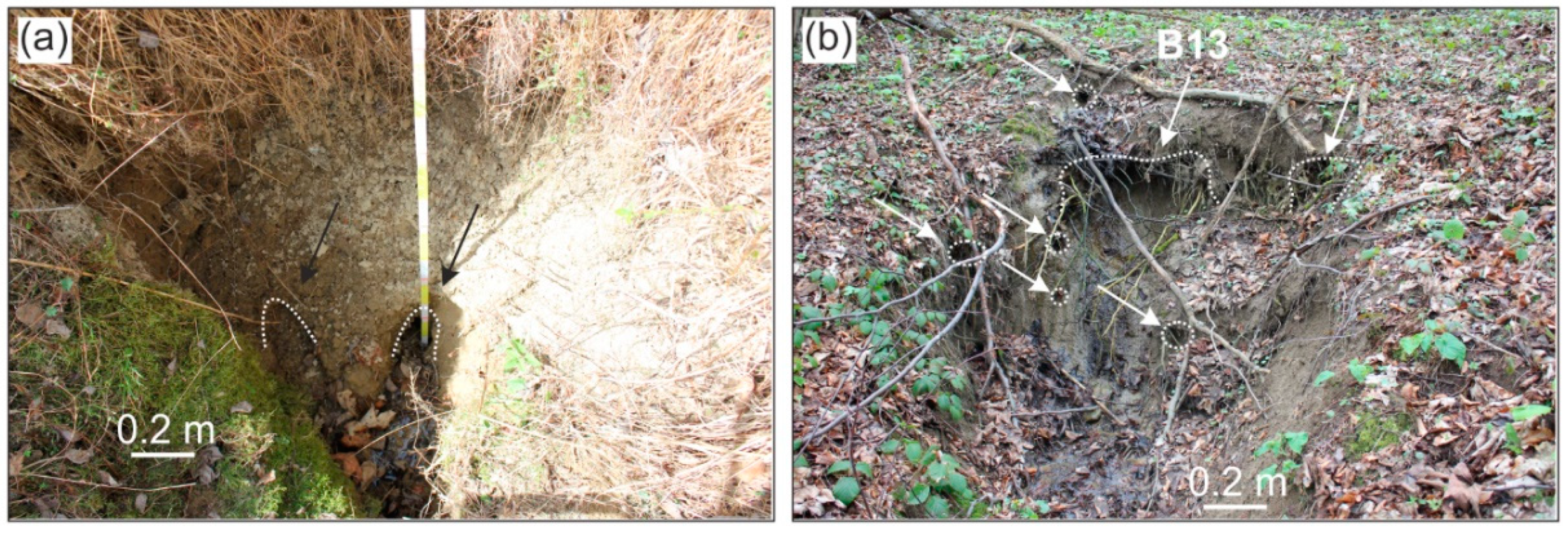
Figure 9.
The complex pipe network of system B13 in site B: (a) The pipe inlets (marked by black arrows) in a sinkhole; (b) The overview of the gully head in site B, where piping system B13 ends (white arrows indicate the pipe outlets; B13 marks the main pipe outlet).
Figure 9.
The complex pipe network of system B13 in site B: (a) The pipe inlets (marked by black arrows) in a sinkhole; (b) The overview of the gully head in site B, where piping system B13 ends (white arrows indicate the pipe outlets; B13 marks the main pipe outlet).

Figure 10.
Surface indicators of soil piping in site C: (a) The detailed DEM of site C; (b) The overview of site C with piping system C11 (white dotted line indicates the potential subsurface pipe); (c) Soil pipe outlet (Video S1); (d) The lower part of site C with closed (sagging) depression and blind gully; (e) Blind gully. Number 1 (a) indicates the blind gully presented in the photo (d,e). Signature C11 indicates a pipe on (a,b).

Figure 11.
Spatial visualization of soil pipe network of site C based on longitudinal radargrams GPR_C1 to GPR_C5 with transverse radargram GPR_C6 in the bottom and radargram GPR_C7 that followed surface indicators of piping system C11 (to check the location of radargrams see Figure 3). Black signatures GPR_C1 to GPR_C7 refer to profile numbers (Figure 3), whereas white numbers refer to the pipe number (C11). Red circles indicate places where a pipe is both visible on the surface (i.e., sagging of ground or collapse) and on radargrams (i.e., reflected as hyperbolas), and black circles indicate places where is clear reflection on radargrams, but there are no surface indicators.


Table 1.
Basic information on GPR surveys at the study sites.
| Catchment | Study Site | Area of Study Site (m2) | GPR Antennas | Depth of Radargrams (m) | Number and Length of Radargrams | |
|---|---|---|---|---|---|---|
| Longitudinal | Transverse | |||||
| Bereźnica | A | 1900 | 500 MHz | 3.2 | 1 (57 m) | 13 (22–30 m) |
| Bereźnica | B | 5800 | 500 MHz | 3.2 | 2 (84–95 m) | 13 (45–60 m) |
| Cisowiec | C | 850 | 800 MHz | 2.0 | 5 (45 m) | 1 (22.5 m) |
Table 2.
Possible resolution in soil pipe detection achieved in different types of soils while using GPR antennas of different frequencies. The wave velocity and dielectric constant are based on Robinson et al. [30].
Table 2.
Possible resolution in soil pipe detection achieved in different types of soils while using GPR antennas of different frequencies. The wave velocity and dielectric constant are based on Robinson et al. [30].
| Parameters | Dry Clayey Soils | Wet Clayey Soils | Unsaturated Silt | Saturated Silt | ||||
|---|---|---|---|---|---|---|---|---|
| Wave velocity (m ns−1) | 0.1897 | 0.0707 | 0.105 | 0.06 | ||||
| Dielectric constant ε | 2.5 | 18 | 3.8 | 26 | ||||
| Frequency (MHz) | λ (m) | R (m) | λ (m) | R (m) | λ (m) | R (m) | λ (m) | R (m) |
| 100 | 1.90 | 0.47 | 0.71 | 0.18 | 1.05 | 0.26 | 0.60 | 0.15 |
| 250 | 0.76 | 0.19 | 0.28 | 0.07 | 0.42 | 0.11 | 0.24 | 0.06 |
| 500 | 0.38 | 0.095 | 0.14 | 0.035 | 0.21 | 0.053 | 0.12 | 0.030 |
| 800 | 0.24 | 0.059 | 0.09 | 0.022 | 0.13 | 0.033 | 0.08 | 0.019 |
λ—wavelength; R—resolution.
© 2019 by the authors. Licensee MDPI, Basel, Switzerland. This article is an open access article distributed under the terms and conditions of the Creative Commons Attribution (CC BY) license (http://creativecommons.org/licenses/by/4.0/).
Share and Cite
MDPI and ACS Style
Bernatek-Jakiel, A.; Kondracka, M. Detection of Soil Pipes Using Ground Penetrating Radar. Remote Sens. 2019, 11, 1864. https://0-doi-org.brum.beds.ac.uk/10.3390/rs11161864
AMA Style
Bernatek-Jakiel A, Kondracka M. Detection of Soil Pipes Using Ground Penetrating Radar. Remote Sensing. 2019; 11(16):1864. https://0-doi-org.brum.beds.ac.uk/10.3390/rs11161864
Chicago/Turabian StyleBernatek-Jakiel, Anita, and Marta Kondracka. 2019. "Detection of Soil Pipes Using Ground Penetrating Radar" Remote Sensing 11, no. 16: 1864. https://0-doi-org.brum.beds.ac.uk/10.3390/rs11161864
Note that from the first issue of 2016, this journal uses article numbers instead of page numbers. See further details here.