ℓ_p-ICP Coastline Inflection Method for Geolocation Error Estimation in FY-3 MWRI Data

Abstract

Known as input in the Numerical Weather Prediction (NWP) models, Microwave Radiation Imager (MWRI) data have been widely distributed to the user community. With the development of remote sensing technology, improving the geolocation accuracy of MWRI data are required and the first step is to estimate the geolocation error accurately. However, the traditional method, such as the coastline inflection method (CIM), usually has the disadvantages of low accuracy and poor anti-noise ability. To overcome these limitations, this paper proposes a novel ${\ell }_p$ iterative closest point coastline inflection method (${\ell }_p$-ICP CIM). It assumes that the field of views (FOVs) across the coastline can degenerate into a step function and employs an ${\ell }_p(0\le p<1)$ sparse regularization optimization model to solve the coastline point. After estimating the coastline points, the ICP algorithm is employed to estimate the corresponding relationship between the estimated coastline points and the real coastline. Finally, the geolocation error can be defined as the distance between the estimated coastline point and the corresponding point on the true coastline. Experimental results on simulated and real data sets show the effectiveness of our method over CIM. The accuracy of the geolocation error estimated by ${\ell }_p$-ICP CIM is up to $0.1$ pixel, in more than $90\%$ of cases. We also show that the distribution of brightness temperature near the coastline is more consistent with the real coastline and the average geolocation error is reduced by $63\%$ after geolocation error correction.

1. Introduction

FY-3 satellites are the second generation of Chinese polar orbital series meteorological satellites. Up to now, four satellites of the FY-3 series, i.e., FY-3A, FY-3B, FY-3C and FY-3D have been launched, where the last three satellites are still in orbit [1]. FY-3 series satellites are equipped with various instruments in the visible, infrared and microwave bands, which provide abundant information for global climate prediction and weather prediction. The Microwave Radiation Imager (MWRI) is an important remote sensor onboard the FY-3 meteorological satellite, including 10 channels in five frequency bands: 10.65, 18.7, 23.8, 36.5 and 89.0 GHz V/H. The MWRI radiometer weighs 175 kg and consumes 125 W of power. It consists of an offset parabolic main reflector of size 977.4 mm × 897.0 mm and four independent feed horns. The MWRI calibration system is designed as an end-to-end all-optical calibration system. Two quasi-optical mirrors with a diameter of 860 mm and 1300 mm installed in the heat source and cold air observation positions are used to obtain cold/thermal calibration observation data. MWRI acquired six cold/heat source observations and 254 observations from Earth scenes within 1.8 s of each scan cycle. The MWRI frequencies, polarization, ground resolution, bandwidth, beamwidth, and noise-equivalent temperature sensitivity $\left(NE\mathsf{\Delta }T\right)$ are provided in

Table 1. FY-3C MWRI instrument characteristics.

Frequency (GHz)	10.65	18.7	23.8	36.5	89
Polarization	V/H	V/H	V/H	V/H	V/H
Bandwidth (MHz)	180	200	400	400	3000
Sensitivity (K)	0.5	0.5	0.5	0.5	0.8
Samples/scan	254
Beam Width	${2.3}^{\circ }$	${1.35}^{\circ }$	${1.22}^{\circ }$	${0.81}^{\circ }$	${0.41}^{\circ }$
Ground Resolution (km)	$51\times 85$	$30\times 50$	$27\times 45$	$18\times 30$	$9\times 15$
Scan Mode	Conical scanning
Orbit Width	1400 km
Viewing Angle (${}^{\circ }$)	45
Integration time (ms)	15.0	10.0	7.5	5.0	2.5
Sampling Interval	2.08 ms
Sampling angle	${0.4111}^{\circ }$
Scan period	1.8s

. The main task of MWRI is to provide multi-purpose imagery with emphasis on precipitation. According to the characteristics of MWRI, a variety of engineering functions have been developed, including precipitation intensity at surface (liquid or solid), sea-ice cover, wind speed over the surface (horizontal), sea surface temperature, cloud liquid water (CLW) total column, snow cover and so on [2,3].

The MWRI data can be used in quantitative remote sensing applications, such as disastrous weather detection and numerical weather prediction. In these quantitative applications, high-precision geolocation and radiometric calibration are the primary conditions. However, due to the instability of satellite attitude, the observation position of satellite in orbit will be inconsistent with the actual position. It is called geolocation error, which is one of the most important factors affecting the quantitative application of satellite remote sensing data [4,5,6,7,8].

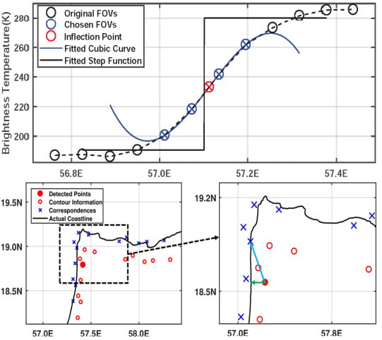
Up to now, several methods have been proposed for the geolocation error estimation of MWRI, such as coastline inflection point method (CIM) [9,10,11,12] and node differential method (NDM) [13,14,15,16]. The NDM estimates satellite attitude angle error and corrects geolocation error by minimizing the brightness temperature difference between ascending and descending orbit data in the same region. The CIM assumes that the brightness temperature of four continuous field of views (FOVs) across the coastline satisfy the cubic curve equation, and the inflection point of the cubic curve is set as the coastline point. As shown in Figure 1a, four FOVs (blue circles) are first selected and then used to fit a cubic polynomial curve (blue line). The inflection point of the fitted cubic curve is set as the coastline point denoted as a red circle. When the coastline point is estimated, the vertical distance between the estimated coastline point and the real coastline is taken as the geolocation error [14], which is shown as a green arrow in the right enlarged image of Figure 1b.

Due to the simplicity and efficiency, the CIM has attracted considerable attention and been widely applied on many satellites. For example, it has been applied to the Earth Radiation Budget Experiment (ERBE) scanner on the Earth Radiation Budget Satellite (ERBS) and the NOAA-9 spacecraft [14], the Clouds and the Earth’s Radiant Energy System (CERES) scanner [9], the Atmospheric Infrared Sounder (AIRS) on Aqua [10], and the Cloud-Aerosol Lidar Infrared Pathfinder Satellite Observations (CALIPSO) [17]. Recently, Tang applied the CIM to estimate the geolocation error and adjusted the attitude angle of FY-3C according to the geolocation error on FY-3C MWRI data [11].

Despite great success in practical applications, CIM still has some problems to solve. First, the cubic curve cannot show the sudden change of brightness temperature near the coastline well and is also prone to being affected by noise, as shown in Figure 1a. Second, the vertical distance between the coastline point and the real coastline cannot depict the geolocation error accurately. When the coastline is not completely straight, taking the vertical distance from the detected coastline point to the real coastline as geolocation error will lead to wrong results. These two problems are the main factors limiting the accuracy of CIM.

Presently, some advanced algorithms have been proposed to improve the accuracy of CIM. For example, Li et al. [18] proposed an ${\ell }_0$ sparse approximation model for geolocation error estimation. They use the jump point of the step function to estimate the true coastline point. Although it improves the geolocation accuracy, it does not solve the problems mentioned above. Therefore, the ${\ell }_p$-ICP CIM algorithm was proposed in order to further improve the accuracy. To solve the first problem, we increase the number of FOVs used in solving the coastline point to alleviate the effect of noise, and propose a novel ${\ell }_p(0\le p<1)$ sparse regularization optimization model to estimate the original brightness temperature curve. Considering that the temperature on both sides of the coastline point should have a step change, the original ideal brightness temperature curve is modeled as a step function (black line in Figure 1a). By assuming that the observed brightness temperature curve is the convolution of the original ideal brightness temperature curve (i.e., a step function) with an unknown kernel function, the step function can be solved according to an ${\ell }_p(0\le p<1)$ sparse regularization optimization model [18,19,20,21,22], and the step point of the step function is considered the coastline point.

To solve the second problem, we consider the neighborhood information or contour information of the estimated coastline point (neighboring points are shown as red hollow points in Figure 1b), and assume that there is a rigid transformation [23] between the real coastline and the estimated coastline. Here, the Iterative Closest Point (ICP) algorithm [24,25] is used to estimate the rigid transformation. When the rigid transformation is estimated, the corresponding points of neighboring coastline points can be obtained, as shown in blue forks in Figure 1b). For the detected coastline point (red solid point), we can find the corresponding point by the ICP algorithm. Note that the corresponding point does not necessarily coincide with the real coastline. Thus, we find a point on the real coastline that is closest to the corresponding point, which is denoted as the corresponding point on the real coastline. Finally, the distance between the detected coastline point and the corresponding point on the real coastline is defined as geolocation error, which is shown as a light blue arrow in the right enlarged image of Figure 1b.

The main contributions of this paper are as follows:

• According to the characteristics of FY-3 MWRI data, we model the observed brightness temperature curve as the convolution of a step function with an unknown kernel function and propose a novel ${\ell }_p$ sparse regularization optimization model to solve the step function and locate the coastline point. In addition, we provide a fast solution based on the fast Fourier transform (FFT).
• We propose a new definition of geolocation error by introducing the contour information of the coastline and employing the ICP algorithm to estimate the rigid transformation between the real coastline and the estimated coastline points.

This paper is organized as follows: Section 2 introduces the method proposed in this paper in detail. Section 3 provides the experimental results and analysis, while Section 4 provides a discussion. The summary and conclusions are given in Section 5.

2. Proposed Method

The proposed method includes the following two parts: (1) locating the coastline point by the ${\ell }_p$ sparse regularization optimization model; and (2) finding the corresponding points between the coastline point and the real coastline and calculating the geolocation error.

To accurately describe the variation of brightness temperature near the coastline, we increase the number of FOVs per group from 4 to 12. These FOVs should satisfy the following conditions [14]:

(1)

No unusual terrain features, such as lakes and mountains, next to the coastline.

(2)

Probable high thermal contrast between land and water, and the maximum temperature difference is obtained between the 6th and 7th FOV.

(3)

Interesting coastline. A coastline with regular curves, peninsulas, and bays is most useful.

(4)

Cloudless disturbance.

2.1. Data Interpolation

In order to improve the accuracy, it is necessary to interpolate the 12 selected FOVs before calculating the coastline point. In this paper, an interpolation scheme is designed according to the characteristics of MWRI data. The latitude, longitude and brightness temperature of 12 selected FOVs are recorded as $La{t}_0$, $Ln{g}_0$, $g_0$. According to the required interpolation accuracy, the original longitude and latitude are interpolated linearly, and recorded as $La{t}_1$, $Ln{g}_1$. The brightness temperature is interpolated by 0 and reshaped to a column vector as $g_1$. Let g be the brightness temperature value to be interpolated with the same dimension as $g_1$. The following optimization model is established:

$$arg\underset{g}{min}\parallel Ag-g_1{\parallel }_2^2+\mu {\parallel Kg\parallel }_2^2,$$

(1)

where A is a sparse matrix formed by zeroing the position on the diagonal line of the unit matrix corresponding to the position, where $g_1$ is zero. ${\parallel ·\parallel }_2$ represents 2 norm. K is a sparse matrix with the same dimension as A: $K=[1,-2,1,0,\dots ,0;0,1,-2,1,0,\dots ,0;\dots ]$. $\mu$ is a regularization parameter for balance [26]. The first term in Equation (1) is the data fidelity term, which ensures the similarity between g and the original observed data [20,27]. The second part is the smoothing term. When the resolution of g is improved, it guarantees the smoothness of g (non-smoothness means low resolution). The solution of model (1) is given by the following equation:

$$g={[A^{T}A+\mu K^{T}K]}^{-1}{A}^T{g}_1.$$

(2)

Given 12 FOVs, we can use the interpolation method to generate many points. It should be noted that 12 selected FOVs refer to the brightness temperature values across the coastline rather than the point on the coastline. The temperature variation curve around the coastline can be considered as a smooth curve.

2.2. ${\ell }_p$ Sparse Regularization Optimization Model

In this paper, we assume that the observed brightness temperature signal is convoluted by a step function and an unknown Equation (convolution kernel). The step point (where the value of step function mutates) of the step function is considered to be the coastline point. The ${\ell }_p$ sparse regularization optimized model is used to restore the step function. The previous interpolation results are brought into this model to solve the coastline point.

Let the observed signal (interpolation fitting curve) be g, the original signal be f, and the convolution kernel be h. The subscript n represents the n-th sample. Because the derivative of f is highly sparse, we use ${\ell }_p(0\le p<1)$ norm to restrict its sparsity. Based on the above assumptions, the ${\ell }_p$ sparse regularization model was proposed:

$$\underset{f,h}{min}\left\{\sum _n{\left({(f\otimes h)}_n-g_n\right)}^2+{\phi \parallel \partial h\parallel }_2^2+\lambda {\parallel \partial f\parallel }_p^p\right\},$$

(3)

where ⊗ represents convolution operator, ∂ represents gradient operator, and ${\parallel ·\parallel }_p$ represents p norm. The first part of Equation (3) guarantees the structural similarity between $f\otimes h$ and g. The second part guarantees the smoothness of h, and $\phi$ is the regularization parameter. The third part restricts the sparsity of the gradient of f, and $\lambda$ is a regularization parameter [28].

Since the original h and f are both unknown, we use the iterative blind deconvolution (IBD) algorithm [29,30,31] to solve the regularization model. The optimization problem involves two variables, f and h, which can be solved by alternating optimization the following two equations:

$$h^j=\underset{h}{min}\left\{\sum _n{\left({(f^j\otimes h)}_n-g_n\right)}^2+\phi {\parallel \partial h\parallel }_2^2\right\}$$

(4)

and

$$f^{j+1}=\underset{f}{min}\left\{\sum _n{\left({(f\otimes h^j)}_n-g_n\right)}^2+\lambda {\parallel \partial f\parallel }_p^p\right\},$$

(5)

where j denotes the number of iterations. To speed up the convergence speed, $\lambda$ is set as a variable parameter. Initially, $\lambda$ is set to a small value ${\lambda }_0$. Given a step size ${\kappa }_1$, and $\lambda$ is updated after each iteration: ${\lambda }^{j+1}={\lambda }^j\times {\kappa }_1$. When step size ${\kappa }_1>1$, $\lambda$ will increase with iterations. Given a threshold ${\lambda }_{max}$, the iteration stops until $\lambda >{\lambda }_{max}$. In our experiment, ${\lambda }_0$, ${\lambda }_{max}$, ${\kappa }_1$, $\phi$ are set to $0.09$, 100, $1.5$, 5, respectively. This method has been proved to be effective in accelerating convergence [31,32,33,34]. In the following, we focus on solving models (4) and (5).

2.2.1. Minimizing Model (4)

Because the model (4) is convex, it has a global optimal solution. Considering the existence of gradient operator and convolution operator in model (4), the computational process can be accelerated through the FFT [28]. Fixed $f^j$, $h^j$ can be solved by:

$$h^j={\mathcal{F}}^{-1}\left(\frac{\mathcal{F}\left(g\right)\circ {\mathcal{F}}^{*}\left(f^j\right)+\phi \mathcal{F}(\partial )\circ {\mathcal{F}}^{*}(\partial )}{\mathcal{F}\left(f^j\right)\circ {\mathcal{F}}^{*}\left(f^j\right)+\phi \mathcal{F}(\partial )\circ {\mathcal{F}}^{*}(\partial )}\right),$$

(6)

where $\mathcal{F}$, ${\mathcal{F}}^{-1}$, * and ∘ denote the FFT operator, the inverse FFT operator, the complex conjugate and the componentwise multiplication, respectively. Note that the addition and division in Equation (6) are also component-wise operators; the calculation speed is much faster than that in the original space.

2.2.2. Minimizing Model (5)

It should be noted that model (5) is non-convex [30] and is difficult to be optimized directly. To date, a number of algorithms have been proposed for solving this problem [33,35,36,37,38,39,40,41]. In this paper, we apply the Generalized Iterated Shrinkage algorithm (GISA) [35] to solve model (5). For this purpose, a new variable $d=\partial f$ is introduced and the model (5) is rewritten as:

$$\underset{f,d}{min}\left\{\sum _n{\left({(f\otimes h^j)}_n-g_n\right)}^2+\frac{\eta \lambda }{2}{\parallel \partial f-d\parallel }_2^2+\lambda {\parallel \partial f\parallel }_p^p\right\},$$

(7)

where $\eta$ is a variable parameter. When $\eta \to \infty$, model (7) is equivalent to model (5). Note that model (7) contains two variables f and d, an alternating optimization of f and d is introduced as follows:

Step 1: 

fixed${\mathit{f}}^{\mathit{j},\mathit{i}}$, solving${\mathit{d}}^{\mathit{i}}$.

Fixing $f^{j,i}$, and denoting $d^{ref}=\partial f$, $d^i$ can be solved by the following sub-problem:

$$\underset{d}{min}\left\{\frac{\eta }{2}\parallel d-d^{ref}{\parallel }_2^2+{\parallel d\parallel }_p^p\right\}.$$

(8)

The generalized soft-thresholding (GST) function can be used to solve the sub-problem (8), and the corresponding solution $d^i$ is:

$$d^i=T_p^{GST}\left(d_i^{ref};\frac{1}{\eta }\right),$$

(9)

where $T_p^{GST}$ is a soft threshold function:

$$T_p^{GST}(y;\lambda )=\left\{\begin{array}{c}\hfill 0,if\left|y\right|\le {\tau }_p^{GST}\left(\lambda \right),\\ \hfill sgn\left(y\right)S_p^{GST}\left(\right|y|;\lambda ),if\left|y\right|>{\tau }_p^{GST}\left(\lambda \right),\end{array}\right.$$

(10)

where ${\tau }_p^{GST}\left(\lambda \right)$ is defined by:

$${\tau }_p^{GST}\left(\lambda \right)={\left(2\lambda (1-p)\right)}^{\frac{1}{2-p}}+\lambda p{\left(2\lambda (1-p)\right)}^{\frac{p-1}{2-p}}$$

(11)

and $S_p^{GST}$ can be solved by:

$$S_p^{GST}(y;\lambda )-y+\lambda p{\left(S_p^{GST}(y;\lambda )\right)}^{p-1}=0.$$

(12)

Like the soft-thresholding   function [42], the GST function also involves a thresholding rule $T_p^{GST}(y;\lambda )=0$ when $\left|y\right|\le {\tau }_p^{GST}\left(\lambda \right)$ and a shrinkage   rule $T_p^{GST}(y;\lambda )=sgn\left(y\right)S_p^{GST}\left(\right|y|;\lambda )$, when $\left|y\right|>{\tau }_p^{GST}\left(\lambda \right)$.   Compared with the thresholding function in [33], the GST function adopted a different thresholding value ${\tau }_p^{GST}\left(\lambda \right)$ and can always find the correct solution to the simple ${\ell }_p$-minimization problem. Thus, GST can be regarded as a better generalization of soft-thresholding   for ${\ell }_p$-minimization.

Step 2: 

fixed${\mathit{d}}^{\mathit{i}}$, solving${\mathit{f}}^{\mathit{j},\mathit{i}}$.

For each fixed $d^i$, $f^{j,i}$ can be solved by the following sub-problem:

$$\underset{f}{min}\left\{\sum _n{\left({(f\otimes h^j)}_n-g_n\right)}^2+\frac{\eta \lambda }{2}{\parallel \partial f-d^i\parallel }_2^2\right\}.$$

(13)

Similar to model (4), the solving process of model (13) can be transformed into the Fourier domain. With fixed $d^i$, $f^{j,i}$ can be solved by:

$$f^{j,i}={\mathcal{F}}^{-1}\left(\frac{\mathcal{F}(\eta \frac{\lambda }{2}\partial d)+{\mathcal{F}}^{*}\left(h\right)\circ \mathcal{F}\left(g\right)}{\eta \frac{\lambda }{2}\mathcal{F}({\partial }^T\partial )+{\mathcal{F}}^{*}\left(h\right)\circ \mathcal{F}\left(h\right)}\right).$$

(14)

Step 3: 

back to step 1 until convergence.

The solution of model (7) can be obtained by alternatively updating f and d. Similar to the parameter setting of $\lambda$, $\eta$ is also set as a variable parameter to accelerate convergence. Let ${\eta }_0$, ${\eta }_{max}$, ${\kappa }_2$ be the initial value, threshold and step size, respectively. In the experiment, ${\eta }_0$, ${\eta }_{max}$, ${\kappa }_2$ are set as $1.4$, $2^{18}$, $1.1$, respectively.

Algorithm 1 gives an overview of the proposed ${\ell }_p$ sparse regularization optimization model. It will output a step function which can be considered as an ideal brightness temperature signal and the step point of step function is taken as the coastline point.

Algorithm 1${\ell }_p$ Sparse Regularization Optimization Model

Input: 12 FOVs data, parameters $\phi$, ${\lambda }_0$, ${\lambda }_{max}$, ${\eta }_0$, ${\eta }_{max}$, and rates ${\kappa }_1$, ${\kappa }_2$. Output: Step function f. 1: Fit interpolation curve g by Equation (2); 2: Initialization:$f^1\leftarrow f^0$, $\lambda \leftarrow {\lambda }_0$, $j\leftarrow 1$; 3: repeat 4:  With $f^j$, solve $h^j$ by Equation (6); 5:  Initialization: $f^{j,1}\leftarrow f^j$, $\beta \leftarrow {\beta }_0$, $i\leftarrow 1$; 6:  repeat 7:   With $f^{j,i}$, solve for $d^i$ in Equation (9); 8:   With $d^i$, solve for $f^{j,i+1}$ in Equation (14); 9:   Set $\eta \leftarrow {\kappa }_2\times \eta$, $i\leftarrow i+1$; 10:  until $\eta \ge {\eta }_{max}$ 11:  Set $f^{j+1}\leftarrow f^{j,i}$, $\lambda \leftarrow {\kappa }_1\times \lambda$, $j\leftarrow j+1$; 12: until$\lambda >{\lambda }_{max}$

2.3. Correspondence Point Estimation and Error Calculation

The purpose of this subsection is to find the corresponding points of the detected coastline points on the real coastline. The neighborhood information of detected coastline point is considered in the calculation process. We assume that there are only rotation and displacement transformations (rigid transformations) [23] between the real coastline and the estimated coastline. Thus, the key is to estimate the rigid transformation.

In fact, the real coastline and estimated coastline are composed of two point sets. Let the real coastline be the target point set $Q_m$, the estimated coastline be the source point set $P_n$ (m, n are not necessarily equal) and there is a transformation H between the two point sets. Since we assume that there is only a rigid transformation between them, H can be expressed by the following formula:

$$H=\left[\begin{array}{cc}{R}_{2\times 2}& T_{2\times 1}\\ 0_{1\times 2}& 1\end{array}\right],$$

(15)

where the rotation matrix $R_{2\times 2}$ and translation matrix $T_{2\times 1}$ can be expressed by the following formulas:

$$R_{2\times 2}=\left[\begin{array}{cc}cos\theta & -sin\theta \\ sin\theta & cos\theta \end{array}\right],$$

(16)

$$T_{2\times 1}={\left[\begin{array}{cc}{t}_x& t_y\end{array}\right]}^T,$$

(17)

where $\theta$ denote the rotation angle. $t_x$, $t_y$ represent displacements along x- and y-axes, respectively. The coordinate transformation of $P_i$ and $Q_i$ in two different coordinate systems can be achieved by the following formulas:

$$P_i=R_{2\times 2}\times Q_i+T_{2\times 1},$$

(18)

where $P_i={[x_i,y_i]}^T$, $Q_i={[x_i^{\prime },y_i^{\prime }]}^T$. Submit $P_i$ and $Q_i$ into Equation (18):

$$\left[\begin{array}{c}{x}_i^{\prime }\\ y_i^{\prime }\end{array}\right]=\left[\begin{array}{cc}cos\theta & -sin\theta \\ sin\theta & cos\theta \end{array}\right]\left[\begin{array}{c}{x}_i\\ y_i\end{array}\right]+\left[\begin{array}{c}{t}_x\\ t_y\end{array}\right]$$

(19)

In this paper, the ICP algorithm is used to estimate the rigid transformation due to its simplicity and low computational complexity [24,43,44,45]. The ICP algorithm is an optimal matching method based on a least square method essentially [46,47]. It repeats the process of “determining the set of corresponding points—calculating the optimal rigid body transformation” until a convergence criterion representing the correct matching is satisfied. The purpose of the ICP algorithm is to find the rotation $\left(R_{2\times 2}\right)$ and translation $\left(T_{2\times 1}\right)$ transformation between the target point set and the source point set, so as to minimize the error function E:

$$E(R,T)=\frac{1}{n}\sum _{i=1}^n{\parallel Q_i-(R\times P_i+T)\parallel }^2,$$

(20)

where n is the number of nearest point pairs, $Q_i$ is a point in the target point set Q, $P_i$ is the nearest point corresponding to $Q_i$ in the source point set P, R is the rotation matrix, and T is the translation vector. The specific steps of ICP algorithm are as follows:

(1)

Calculate the corresponding nearest points of each point in P in the point set Q.

(2)

The rigid transformation that minimizes the average distance between the corresponding points mentioned above is obtained, and the translation and rotation parameters are obtained.

(3)

For P, the translation and rotation parameters obtained in the previous step are used to obtain a new set of transformation points.

(4)

If the average distance between the new transformation point set and the reference point set is less than a given threshold, the iteration will be stopped, otherwise the new transformation point set will continue to iterate as a new P until it meets the requirements of the objective function.

In the experiment, we use Global Self-consistent, Hierarchical, High-resolution Shoreline (GSHHS) fine-resolution database (∼40 m resolution) [48] to define the truth coastline. Note that the x-axis and y-axis coordinates of two point sets $P,Q$ are determined by their geographical location. When the rigid transformation is estimated, the corresponding point of the detected coastline point on the GSHHS can be found, and then the geolocation error can be obtained by the distance between them. The detailed process is as follows:

(1)

Denote an estimated coastline point as a, define a neighborhood near a and compute the extreme points of the brightness temperature gradient within the neighborhood, record the extreme points as A. Find the true coastline points corresponding to the neighborhood from the GSHHS and denote them as B. Here, A and B are the estimated and real coastlines, respectively.

(2)

Estimate the rigid transform T from A to B by the ICP algorithm.

(3)

Let A be transformed into C by T, and c is the corresponding point of a in C. Let $d\in B$ be the point with the closest distance to c, and the distance between a and d is taken as the geolocation error.

(4)

Repeat until geolocation error for all points are calculated.

3. Experiments and Results

In this section, we first analyze the causes of geolocation errors, then give the experimental results, and finally show the results of geolocation error correction.

3.1. Geolocation Error Analysis

The geolocation error of MWRI is closely related to the uncertainty of basic measurement data used in the calculation. Satellite position deviation, satellite attitude angles (e.g., pitch, roll, and raw) deviation and instrument installation error are the main sources of geolocation errors. In general, the geolocation error can be classified into dynamic and static errors. Dynamic error sources include thermal deformation and structural deformation of instruments, thermal deformation and structural deformation of satellites, attitude angles and position measurement deviation of satellites. These dynamic errors vary all the time and are difficult to simulate. Static error sources include antenna scanning angle deviation, installation deviation of detector, antenna and instrument, and systematic error of star tracker (stellar position deviation). These static errors are invariable and can be reduced or eliminated by the processing of ground application systems [49,50].

In order to measure geolocation errors, two basic performance indicators (i.e., cross-track error and along-track error) are adopted in this paper [14]. The conversion equation from latitude and longitude coordinates to cross-track and along-track coordinates is:

$$\left(\begin{array}{c}{\epsilon }_c\\ {\epsilon }_a\end{array}\right)=\left(\begin{array}{cc}\pm sin\eta & cos\eta \\ -cos\eta & \pm sin\eta \end{array}\right)\left(\begin{array}{c}{\epsilon }_{\mathsf{\Lambda }}\\ {\epsilon }_{\mathsf{\Phi }}\end{array}\right),$$

(21)

where $\eta$, ${\epsilon }_c$, ${\epsilon }_a$, ${\epsilon }_{\mathsf{\Lambda }}$, ${\epsilon }_{\mathsf{\Phi }}$ represent the spacecraft heading angle, cross-track error, along-track error, longitude error and latitude error, respectively. The upper sign ‘+’ in Equation (21) is used when the scan direction is left to right; otherwise, the lower sign ‘−’ is used. The transformation from latitude and longitude coordinates to cross-track and along-track coordinates is also shown in Figure 2.

3.2. Experimental Results

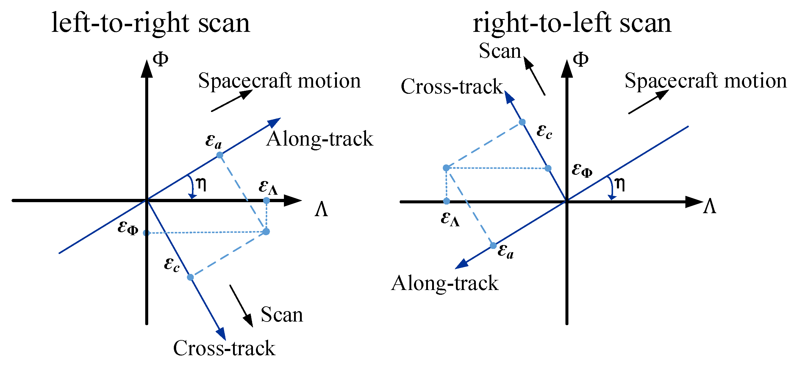
In experiment, the FY-3C MWRI data covering four geographical regions with unique coastline orientations are selected to produce a database of crossing errors, including Libya, South America, Australia and Arabian peninsula as shown in

Table 2. Coordinated Universal Time (UTC) times of FY-3C MWRI data used in the experiment.

Region	Libya	South America	Australia	Arabian Peninsula
Date and UTC Time	201601052022	201601040346	201601061458	201601051840
	201601121950	201601110314	201601081420	201601101847
	201601152034	201601210326	201601121445	201601121808
	201601272008	201601260332	201601221458	201601171814
	201602112026	201602060325	201601221458	201602111845
			201602081438	201602131807
				201602171832
				201602181813
				201602191754

. Their geographical location is shown in Figure 3. These four regions are selected for the following reasons:

• There are obvious temperature differences between ocean and land. For example, in summer, the temperature on land at night is lower than that on water surface, while in the daytime it is just the opposite.
• The selected area should always be in a clear sky because the long-wave radiation value of land and water surface will be very small under the influence of clouds, which should be excluded in the calculation.
• The coastline of the selected area should be regularly distributed, diversified and representative, and the land surface should be uniform. The cloud-free FOV at MWRI 89 GHz data was defined by FY-3C Medium Resolution Spectrum Imager (MERSI) data [11].

Firstly, in order to give the results of geolocation qualitatively, we retrieve the types of land and water according to the results of geolocation calculation in the land and water template database, then superimpose the water-land boundary on the MWRI image, and judge the accuracy of geolocation by the coincidence between the calculated water-land boundary and the actual MWRI image. The overlay maps of the water-land boundary and MWRI images in the Arabian Peninsula at 6:13 p.m. UTC 18 February 2016 and the western coast of Australia at 2:31 p.m. UTC 19 February 2016 are shown in Figure 4. The red points in Figure 4 represent the land-sea boundary. It can be found that the geolocation accuracy of FY-3 MWRI is about one pixel, but there are still geolocation errors at the sub-pixel level.

By using the proposed method, the geolocation errors expressed by latitude and longitude are detected. Note that each geolocation error can only represent the coastline point used to solve the geolocation error rather than the geolocation error of 12 FOVs used to solve the coastline point. Then, the cross- and along-track errors can be calculated by the Equation (21) easily. We compare CIM with our method in terms of mean and standard deviation of geolocation error.

Firstly, the mean and standard deviation of the cross- and along-track errors of each data are calculated, and then the results belonging to the same region are averaged to get the mean and standard deviation of the geolocation errors in each region. Note that there are geolocation errors for each FOV of MWRI data. On average, each MWRI data will get dozens of geolocation errors after applying ${\ell }_p$-ICP CIM. The mean and standard deviation of geolocation errors in four geographical regions are given in

Table 3. Mean and standard deviations of along- and cross-track errors on four geographical regions.

Region		Libya		South America
Error Direction		Cross-Track	Along-Track	Cross-Track	Along-Track
CIM	Mean error	0.0130	0.0258	0.0011	0.0635
	Standard deviation	0.0342	0.0344	0.0315	0.0288
${\ell }_p$-ICP CIM	Mean error	0.0180	0.0916	−0.0033	0.1025
	Standard deviation	0.0268	0.0338	0.0259	0.0239
Region		Australia		Arabian Peninsula
Error Direction		Cross-Track	Along-Track	Cross-Track	Along-Track
CIM	Mean error	0.0030	0.0357	0.0452	0.0516
	Standard deviation	0.0362	0.0370	0.0330	0.0282
${\ell }_p$-ICP CIM	Mean error	0.0022	0.0732	0.0236	0.0981
	Standard deviation	0.0241	0.0408	0.0229	0.0263

. It can be seen that the geolocation errors in both directions of along-track and cross-track estimated by the two methods are approximately the same. They are greater than zero, except for the cross-track errors estimated by our method at the South America data. At the same time, the along-track errors are greater than the cross-track errors. It shows that both methods can reflect the real geolocation error roughly. However, the value of the geolocation error obtained by the two methods are quite different. In the along-track direction, the geolocation errors estimated by ${\ell }_p$-ICP CIM are much larger than those estimated by the CIM, while, in the cross-track direction, the geolocation errors of our method are less than the errors of CIM. Overall, the estimated geolocation errors of ${\ell }_p$-ICP CIM are greater than those of CIM: an averaged increase of $60\%$ for each region. This is mainly due to the fact that the CIM uses the vertical distance between the estimated coastline point and GSHHS as the geolocation error. It is conservative and often causes the underestimation of the geolocation error [5]. In ${\ell }_p$-ICP CIM, we consider the neighborhood information of the coastline point when calculating the geolocation error, and measure the geolocation error by the ICP algorithm. Although the mean value of geolocation errors estimated by ${\ell }_p$-ICP CIM are relatively larger than CIM, they are true geolocation errors.

Figure 5 shows the standard deviations of the cross- and along-track errors of 25 selected MWRI data (as shown in Table 2), respectively. In Figure 5, the circle represents the standard deviation of the geolocation error estimated by ${\ell }_p$-ICP CIM, and the fork represents the standard deviation of the geolocation error estimated by CIM. It is clear that the standard deviation of the geolocation errors obtained by ${\ell }_p$-ICP CIM is much lower than that of CIM: an average reduction of $28\%$. It demonstrates that ${\ell }_p$-ICP CIM is much more stable than CIM. The reasons are:

• Compared with the CIM, ${\ell }_p$ sparse regularization optimization algorithm utilizes more pixel information in solving coastline point, which improves the robustness of the method in estimating the real coastline point when the coastline has irregular distribution and is corrupted by random noise.
• We use the ICP algorithm to measure the geolocation error, which makes it possible to estimate the geolocation error stably and accurately when the coastline is indented.

Furthermore, since the true geolocation error of the operational MWRI data are unknown, it is difficult to measure the accuracy of the estimated geolocation error directly. In this paper, a method is used to evaluate the accuracy of ${\ell }_p$-ICP CIM: we give the operational geolocation results (latitude and longitude) a fixed offset artificially, and then use ${\ell }_p$-ICP CIM and CIM to estimate the geolocation error, respectively. The original geolocation of MWRI can be understood as follows:

original geolocation = correct geolocation + original geolocation error.

After giving an offset, the original geolocation results change:

original geolocation + offset = correct geolocation + original geolocation error + offset.

Therefore,

original geolocation error = geolocation error − offset.

If the estimated geolocation error is accurate, it should be close to the geolocation error. Therefore, the difference between the estimated geolocation error and offset should be close to the original geolocation error, i.e.,

estimated geolocation error - offset ≈ original geolocation error.

Based on the above equation, the computed difference between the estimated geolocation error and offset should be equal to the original geolocation error. This means that, for different offsets, the corresponding differences should be ideally equal.

The FY-3C MWRI data over the coastal region of the Arabian Peninsula at 6:13 p.m. UTC 18 February 2016 is used in this experiment. As shown in

Table 4. The mean error measured by the CIM and ${\ell }_p$-ICP CIM when there are different offsets in the longitude and latitude directions.

	Lng	−0.1	−0.05	0	0.05	0.1
Lat
−0.1		(0.0429, −0.0349)	(0.0197, −0.0458)	(0.0124, −0.0272)	(0.0429, −0.0349)	(0.0090, 0.0147)
−0.05		(0.0660, −0.0413)	(0.0533, −0.0502)	(0.0353, −0.0410)	(0.0176, −0.0161)	(0.0060, 0.0033)
0		(0.0852, −0.0380)	(0.0636, −0.0525)	(0.0551, −0.0510)	(0.0373, −0.0307)	(0.0271, −0.0088)
0.05		(0.0336, −0.0857)	(0.0478, −0.0686)	(0.0556, −0.0586)	(0.0585, −0.0406)	(0.0493, −0.0249)
0.1		(−0.0041, −0.1178)	(−0.0023, −0.0864)	(0.0261, −0.0579)	(0.0491, −0.0471)	(0.0453, −0.0341)
	Lng	−0.1	−0.05	0	0.05	0.1
Lat
−0.1		(−0.0586, −0.1864)	(−0.0596, −0.1376)	(−0.0591, −0.0875)	(−0.0599, −0.0361)	(−0.0588, 0.0105)
−0.05		(−0.0096, −0.1884)	(−0.0096, −0.1381)	(−0.0096, −0.0884)	(−0.0109, −0.0363)	(−0.0109, 0.0115)
0		(0.0351, −0.1840)	(0.0404, −0.1384)	(0.0404, −0.0881)	0.0391, −0.0363)	(0.0391, 0.0119)
0.05		(0.0766, −0.1801)	(0.0904, −0.1381)	(0.0876, −0.0879)	(0.0891, −0.0363)	(0.0891, 0.0119)
0.1		(0.1163, −0.1666)	(0.1290, −0.1326)	(0.1376, −0.0879)	(0.1391, −0.0363)	(0.1391, 0.0119)

* The upper and lower tables represent the mean of geolocation error estimated by CIM and ${\ell }_p$-ICP CIM, respectively.

, we give offsets of −0.1, −0.5, 0, 0.5 and $0.1$ degrees in the longitude and latitude directions and show the mean geolocation errors measured by the CIM and ${\ell }_p$-ICP CIM, respectively. Note that the estimated geolocation error cannot be compared with the given offsets directly, due to the existence of the geolocation error at original MWRI data. Fixing the longitude (latitude) offset and changing the latitude (longitude) offset, the geolocation errors estimated by ${\ell }_p$-ICP CIM can remain stable in the longitude (latitude) direction and change accurately in the latitude (longitude) direction. However, the geolocation errors estimated by the CIM are inconsistent with the real changes of latitude and longitude. The CIM wrongly estimates the direction of the geolocation error.

Figure 6 shows the differences between the estimated geolocation error and the given offsets intuitively. In principle, the difference between the estimated geolocation error and the given offset should be equal to the original geolocation error of the MWRI data, if the estimated geolocation error is accurate. As shown in Figure 6, for the ${\ell }_p$-ICP CIM, the differences between estimated geolocation errors and the given offsets always remain near the original geolocation error (about ${0.045}^{\circ }$ in latitude, ${-0.085}^{\circ }$ in longitude). However, for the CIM, the differences fluctuate dramatically. This is because CIM does not accurately respond to the change of geolocation when the offset is given on the original geolocation. From the mechanism of CIM, the estimated geolocation error is defined as the nearest distance between the estimated coastline point and the real coastline point. The nearest distance is an overoptimistic metric as shown in Figure 1 and it can easily be affected by noise. Because the estimated geolocation error is inaccurate, the difference between the estimated geolocation error of CIM and offset varies.

It should be noted that Figure 6 shows the difference between the estimated geolocation error and the given offset. Table 4 shows the estimated geolocation error (latitude error, longitude error) when the offset in the longitude or latitude direction changes. Intuitively, when fixing the longitude offset and changing the latitude offset, the estimated longitude error should be unchanged and the latitude error will change. From the lower part of Table 4, for our ${\ell }_p$-ICP CIM algorithm, for each row (latitude offset fixed), the estimated latitude errors are almost unchanged when the longitude offset changes. Meanwhile, we can see that the estimated longitude errors decrease as the decrease of longitude offset and the difference between the estimated longitude error and offset keeps stable at value ${-0.085}^{\circ }$. Similarly, for each column (longitude offset fixed), the estimated longitude errors are almost unchanged when the latitude offset changes, and the difference between the estimated latitude error and offset keeps stable at value ${0.045}^{\circ }$. The longitude error ${-0.085}^{\circ }$ and the latitude error ${0.045}^{\circ }$ can be considered as the original geolocation error in the MWRI data. However, for the CIM, both the estimated latitude and longitude errors do not show these characteristics. The CIM misestimates the value of the geolocation error in both latitude and longitude directions.

3.3. Geolocation Error Correction

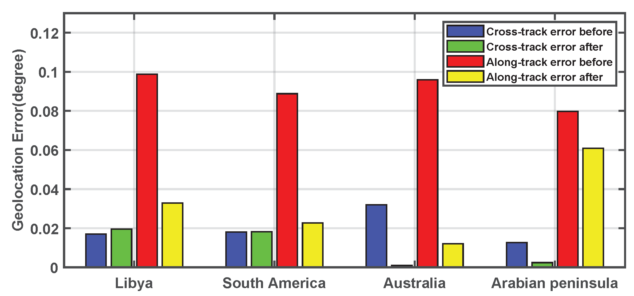
This subsection shows the results of geolocation error correction. Moradi [15] proposed that the geolocation errors of satellite data caused by various factors can be corrected by adjusting the satellite attitude angle. When the geolocation error is obtained, it needs to be converted into a satellite attitude angle error. This process involves the transformation between several coordinate systems. The specific information can be referred to [2]. After adjusting the satellite attitude angle, the MWRI data are relocated. The relocation algorithm provided by the National Satellite Meteorological Center, China Meteorological Administration is used in the process of geolocation error correction. In order to analyze the effect of geolocation error correction comprehensively, the qualitative and quantitative results are given in Figure 7 and Figure 8. The brightness temperature distribution of FY-3C MWRI 89 GHz corresponding to four regions are given in Figure 7 and the black curves represent real coastlines. In detail, Figure 7a shows the brightness temperature distribution over the coastal region of the Libyan at 8:22 p.m. UTC 5 January 2016. Figure 7b shows the brightness temperature distribution over the coastal region of the South American at 3:07 a.m. UTC 22 January 2016. Figure 7c shows the brightness temperature distribution over the coastal region of Australia at 2:26 p.m. UTC 29 January 2016. Figure 7d shows the brightness temperature distributions over the coastal region of the Arabian Peninsula at 6:13 p.m. UTC 18 February 2016. It can be seen from Figure 7 before geolocation errors’ correction that there is a geolocation error towards the southwest in each region. At the same time, the geolocation error in the north–south direction is greater than that in the east–west direction. It is consistent with our previous experimental results. After applying the geolocation error correction to the FY-3C MWRI, the brightness temperature transition is much more natural, with the sharpest gradient occurring at the coastline. It indicates that the geolocation accuracy of MWRI data has been improved.

The quantitative results on the mean geolocation errors before and after correction are given in Figure 8. Blue and red bars denote the cross-track error and along-track error before the correction of geolocation errors, while green and yellow bars denote the cross-track error and along-track error after the correction, respectively. As shown, the geolocation errors are mainly concentrated in the along-track direction: the along-track errors of the four regions are between ${0.08}^{\circ }$ and ${0.11}^{\circ }$, and the cross-track errors are about ${0.02}^{\circ }$. After correction, the geolocation errors have been greatly reduced: in the along-track direction, the geolocation errors of Libya, South America and Australia have been significantly reduced, while that of the Arabian Peninsula is relatively small; in the cross-track direction, the geolocation errors of Australia and the Arabian Peninsula have been significantly reduced. Overall, the average geolocation error of each region was reduced by $63\%$ after correction. It demonstrates the superiority of ${\ell }_p$-ICP CIM from a quantitative point of view.

4. Discussion

This paper improves the original CIM and applies it to estimate the geolocation error of FY-3C MWRI. The CIM used four FOVs crossing the coastline to solve the coastline points. However, the information of four FOVs could not describe the variation of brightness temperature near the coastline very well. It will have a greater impact on the final results, if any FOV data fluctuates due to cloud interference, topographic change or random noise. At the same time, CIM regards the nearest distance from the estimated coastline point to the real coastline as geolocation error, which will lead to underestimation of geolocation error. Therefore, when the coastline is not completely straight and noise exists (which is almost inevitable), the geolocation error estimated by CIM will be less than the real error and the variance is larger. We greatly improve the accuracy of geolocation error estimation through the following two ways: (1) Increasing the number of FOVs per group from 4 to 12 and using an ${\ell }_p(0\le p<1)$ sparse regularization optimization model to improve the stability of an estimated geolocation error; (2) Using an ICP algorithm to determine the ‘corresponding point’ instead of the ‘nearest point’ of the estimated coastline point on the real coastline.

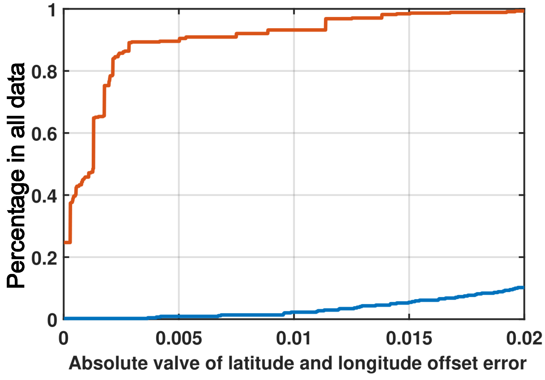
However, the estimated geolocation error’s accuracy is uncertain as the real geolocation error is usually unknown. In Section 3, we compare ${\ell }_p$-ICP CIM with CIM using the strategy of artificially setting offsets on the original location data. In this section, we will continue to use this method to verify the accuracy of our algorithm. The error between the given and estimated latitude and longitude offsets is taken as the criterion to measure the accuracy of the algorithm. The small differences between them indicate a higher accuracy of $\ell p$-ICP CIM. In this section, the MWRI data over the coastal region of the Arabian Peninsula at 6:13 p.m. UTC 18 February 2016 is used in experiments. At the same time, we give the offset from ${-0.1}^{\circ }$ to ${0.1}^{\circ }$ in longitude and latitude respectively in the unit of ${0.01}^{\circ }$, so that we can get 441 pieces of error data. Figure 9 shows the absolute value of the estimated latitude and longitude offset error in a given range as a percentage of all data. The red line in Figure 9 represents ${\ell }_p$-ICP CIM. As shown in Figure 9, the error of longitude and latitude offset estimated by ${\ell }_p$-ICP CIM is very small, and most of the errors are less than ${0.015}^{\circ }$. Specifically, about $90\%$ of the error is less than ${0.005}^{\circ }$, $93\%$ of the error is less than ${0.01}^{\circ }$, and $99\%$ of the error is less than ${0.02}^{\circ }$. This shows that ${\ell }_p$-ICP CIM can estimate the given offset accurately. At the same time, we estimate the accuracy of CIM in the same way. The result is shown by the blue line in Figure 9. It can be seen that the error of CIM is very large, and only about $10\%$ of the estimated offset error does not exceed ${0.02}^{\circ }$. It shows that the accuracy of $\ell p$-ICP CIM is much higher than that of the CIM algorithm.

In order to display the algorithm accuracy more intuitively, we transform the longitude and latitude errors into the pixel errors. The resolution of MWRI image is 9 km × 12 km, and its corresponding latitude and longitude range is about ${0.09}^{\circ }\times {0.11}^{\circ }$ in the Arabian Peninsula. More than $90\%$ of the latitude and longitude offset errors estimated by our algorithm are less than ${0.009}^{\circ }$, as can be seen from the above analysis. Therefore, the accuracy of the geolocation error estimated by ${\ell }_p$-ICP CIM is up to $0.1$ pixel, in more than $90\%$ of cases.

Although our algorithm has achieved a high accuracy in geolocation error estimation, there are still some problems in the process of testing:

• Although the accuracy has been effectively improved, the complexity of our algorithm is higher than CIM. The experiments are performed on a personal computer with an i5-7200U 2.50 GHz Intel processor and 4 GB of RAM. On average, the time required for our algorithm to process a data are 31 s, while the time required for CIM is 3 s in the same running environment. The shortage of computational efficiency leads to obvious disadvantage of our algorithm in dealing with large-scale data.
• When there is no obvious noise, the difference between the coastline points located by ${\ell }_p(0\le p<1)$ sparse regularization optimization model and located by CIM is not obvious (which is natural because they are all sub-pixel level operations), and the difference between the geolocation error estimated by ${\ell }_p$-ICP CIM and CIM is mainly reflected in the process of finding corresponding point.

5. Conclusions

In this paper, we have proposed a novel geolocation error correction method: ${\ell }_p$-ICP CIM for the FY-3 MWRI data. The proposed method mainly includes two parts: the detection of coastline point and the determination of geolocation error. To obtain a robust estimation of coastline point, a novel ${\ell }_p$ sparse regularization optimization model is proposed to solve the coastline point with the use of more FOVs. In the determination of geolocation error, rather than using the vertical distance between the estimated coastline point and the real coastline as the geolocation error, the neighborhood information of the estimated coastline points are considered, and the ICP algorithm is employed to estimate the rigid transformation between the real coastline and the estimated coastline. Finally, the distance between the estimated coastline point and the corresponding point on the true coastline is considered geolocation error.

In the experiment, we compare ${\ell }_p$-ICP CIM with the CIM algorithm. Experimental results demonstrate that our proposed method is more accurate and stable than traditional CIM in the geolocation error estimation of MWRI data. At the same time, we prove that the accuracy of our algorithm is higher than 0.1 pixels in most cases (more than $90\%$), through the designed experiment. Although the accuracy has been improved, the complexity of ${\ell }_p$-ICP CIM has been greatly improved due to the existence of iterative operations, which makes it difficult for us to process a large number of MWRI data. The future work will focus on reducing the complexity of the algorithm and the analysis of geolocation error of a long time series of FY-3 MWRI data, which can help us to better understand the variation of MWRI geolocation error and to correct the geolocation error more accurately [16,51].

References

- Tang, S.H.; Qiu, H.; Ma, G. Review on progress of the Fengyun meteorological satellite. J. Remote Sens. 2016, 15, 842–849. [Google Scholar]
- Yang, H.; Zou, X.L.; Li, X.Q.; Li, N.; You, R.; Wu, S.L. Environmental data records from FengYun-3B Microwave Radiation Imager. IEEE Trans. Geosci. Remote Sens. 2012, 50, 4986–4993. [Google Scholar] [CrossRef]
- Yang, H.; Weng, F.Z.; Lv, L. The FengYun-3 Microwave Radiation Imager on-orbit verification. IEEE Trans. Geosci. Remote Sens. 2011, 49, 4552–4560. [Google Scholar] [CrossRef]
- Guan, M.; Yang, Z.D. Geolocation method for FY-3 MWRI’s remote sensing image. J. Remote Sens. 2009, 13, 463–474. [Google Scholar]
- Wang, L.; Tremblay, D.A.; Han, Y.; Esplin, M.; Hagan, D.E.; Predina, J.; Suwinski, L.; Jin, X.; Chen, Y. Geolocation assessment for CrIS sensor data records. J. Geophys. Res. Atmos. 2013, 118, 12690–12704. [Google Scholar] [CrossRef]
- Poe, G.A.; Uliana, E.A.; Gardiner, B.A.; von Rentzell, T.E.; Kunkee, D.B. Geolocation error analysis of the special sensor microwave imager/sounder. IEEE Trans. Geosci. Remote Sens. 2008, 46, 913–922. [Google Scholar] [CrossRef]
- Wolfe, R.E.; Lin, G.; Nishihama, M.; Tewari, K.P.; Tilton, J.C.; Isaacman, A.R. Suomi NPP VIIRS prelaunch and on-orbit geometric calibration and characterization. J. Geophys. Res. Atmos. 2013, 118, 11508–11521. [Google Scholar] [CrossRef]
- Guan, M.; Yang, Z.D. Application of on-board GPS data and high-precision orbit model to polar satellites orbits calculation. J. Appl. Meteor. Sci. 2007, 18, 748–753. [Google Scholar]
- Smith, G.L.; Priestley, K.J.; Hess, P.C.; Currey, C.; Spence, P. Validation of geolocation of measurements of the Clouds and the Earth’s Radiant Energy System (CERES) scanning radiometers aboard three spacecraft. J. Atmos. Ocean. Technol. 2009, 26, 2379–2391. [Google Scholar] [CrossRef]
- Gregorich, D.T.; Aumann, H.H. Verification of AIRS boresight accuracy using coastline detection. IEEE Trans. Geosci. Remote Sens. 2003, 41, 298–302. [Google Scholar] [CrossRef]
- Tang, F.; Zou, X.L.; Yang, H. Estimation and Correction of Geolocation Errors in FengYun-3C Microwave Radiation Imager Data. IEEE Trans. Geosci. Remote Sens. 2016, 54, 407–420. [Google Scholar] [CrossRef]
- Purdy, W.; Gaiser, P.; Poe, G.; Uliana, E.; Meissner, T.; Wentz, F. Geolocation and pointing accuracy analysis for the WindSat sensor. IEEE Trans. Geosci. Remote Sens. 2006, 44, 496–505. [Google Scholar] [CrossRef] [Green Version]
- Tang, F.; Dong, H.J.; Li, N.; Liu, C.H. Geolocation errors and correction of FY-3B microwave radiation imager measurement. J. Remote Sens. 2016, 20, 1342–1351. [Google Scholar]
- Hoffman, L.H.; Weaver, W.L.; Kibler, J.F. Calculation and Accuracy of ERBE Scanner Measurement Locations; Technical Report; NASA/TP-2670; NASA Langley Research Center: Hampton, VI, USA, 1987; 34p.
- Moradi, I.; Meng, H.; Ferraro, R.R.; Bilanow, S. Correcting geolocation errors for microwave instruments aboard NOAA satellites. IEEE Trans. Geosci. Remote Sens. 2013, 15, 3625–3637. [Google Scholar] [CrossRef]
- Bers, W.S.M. Improved geolocation and earth incidence angle information for a fundamental climate data record of the SSM/I sensors. IEEE Trans. Geosci. Remote Sens. 2013, 51, 1504–1513. [Google Scholar]
- Currey, J.C. Geolocation Assessment Algorithm for CALIPSO Using Coastline Detection; Technical Report; NASA/TP-2002-211956; National Aeronautics and Space Administration (NASA) Langley Research Center: Hampton, VA, USA, 2002; 27p.
- Li, W.F.; Luo, Z.C.; Liu, C.B.; Liu, J.Z.; Shen, L.J.; Xie, Q.W.; Han, H.; Yang, L. ℓ0 Sparse Approximation of Coastline Inflection Method on FY-3C MWRI Data. IEEE Geosci. Remote Sens. Lett. 2019, 16, 85–89. [Google Scholar] [CrossRef]
- Sun, W.W.; Tian, L.; Xu, Y. Fast and robust self-representation method for hyperspectral band selection. IEEE J. Sel. Top. Appl. Earth Observ. Remote Sens. 2017, 10, 5087–5098. [Google Scholar] [CrossRef]
- Sun, W.W.; Du, Q. Graph-regularized fast and robust principal component analysis for hyperspectral band selection. IEEE Trans. Geosci. Remote Sens. 2018, 56, 3185–3195. [Google Scholar] [CrossRef]
- Peng, J.; Li, L.; Tang, Y.Y. Maximum likelihood estimation based joint sparse representation for the classification of hyperspectral remote sensing images. IEEE Trans. Neural Netw. Learn. Syst. 20019, 30, 1790–1802. [Google Scholar] [CrossRef]
- Peng, J.; Sun, W.; Du, Q. Self-paced joint sparse representation for the classification of hyperspectral images. IEEE Trans. Geosci. Remote Sens. 2019, 57, 1183–1194. [Google Scholar] [CrossRef]
- Yu, C.; Chen, X.; Yin, L.; Shu, C.; Zhao, L.; Han, H. Image deformation based on contour using moving integral least squares. IET Image Process. 2019, 12, 152–160. [Google Scholar] [CrossRef]
- Chen, Y.; Medioni, G. Object Modeling by Registration of Multiple Range Images. Image Vis. Comput. 1992, 10, 145–155. [Google Scholar] [CrossRef]
- Besl, P.J.; Mckay, N.D. A Method for registration of 3D shapes. Nat. Rev. Neurosci. 1992, 14, 239–256. [Google Scholar]
- Peng, J.T.; Du, Q. Robust joint sparse representation based on maximum correntropy criterion for hyperspectral image classification. IEEE Trans. Geosci. Remote Sens. 2017, 55, 7152–7164. [Google Scholar] [CrossRef]
- Xie, Q.W.; Mita, S. Integration of optical flow and Multi-Path-Viterbi algorithm for stereo vision. Int. J. Wavelets Multiresolut. Inf. Process. 2017, 15, 1750022. [Google Scholar] [CrossRef]
- Xie, Q.W.; Long, Q.; Mita, S. Image fusion based on multi-objective optimization. Int. J. Wavelets Multiresolut. Inf. Process. 2014, 12, 1450017. [Google Scholar] [CrossRef]
- Shalvi, O.; Weinstein, E. Super-exponential methods for blind deconvolution. IEEE Trans. Infrom. Theory 1993, 39, 504–519. [Google Scholar] [CrossRef]
- Krishnan, D.; Tay, T.; Fergus, R. Blind deconvolution using a normalized sparsity measure. IEEE CVPR 2011, 42, 233–240. [Google Scholar]
- Wang, Y.L.; Yang, J.F.; Yin, W.T.; Zhang, Y. A new alternating minimization algorithm for total variation image reconstruction. SIAM J. Imaging Sci. 2008, 1, 248–272. [Google Scholar] [CrossRef]
- Xie, Q.W.; Ma, C.; Guo, C. Image fusion based on the △−1 − TV0 energy function. Trends Cell Biol. 2014, 16, 6099–6115. [Google Scholar]
- She, Y. Thresholding-based iterative selection procedures for model selection and shrinkage. Electron. J. Stat. 2009, 384–415. [Google Scholar] [CrossRef]
- Sun WeiWei, D.Q. Hyperspectral Band Selection: A Review. IEEE Geosci. Remote Sens. Mag. 2019, 2, 118–139. [Google Scholar] [CrossRef]
- Zou, W.M.; Meng, D.Y.; Zhang, L. A Generalized Iterated Shrinkage Algorithm for Non-convex Sparse Coding. In Proceedings of the IEEE International Conference on Computer Vision (ICCV), Sydney, Australia, 1–8 December 2013; pp. 217–224. [Google Scholar]
- Cho, T.; Zitnick, C.; Joshi, N.; Kang, S.; Szeliski, R.; Freeman, W. Image restoration by matching gradient distributions. IEEE T-PAMI 2012, 34, 683–694. [Google Scholar]
- She, Y.Y. An iterativeal gorithm for fitting nonconvex penalized generalized linear models with grouped predictors. Comput. Stat. Data Anal. 2012, 56, 2976–2990. [Google Scholar] [CrossRef]
- Chartrand, R. Exact reconstruction of sparse signals via nonconvex minimization. IEEE Signal Process. Lett. 2007, 14, 707–710. [Google Scholar] [CrossRef]
- Chartrand, R.; Yin, W. Iteratively reweighted algorithms for compressive sensing. In Proceedings of the 2008 IEEE International Conference on Acoustics, Speech and Signal Processing, Las Vegas, NV, USA, 31 March–4 April 2008; pp. 3869–3872. [Google Scholar]
- Krishnan, D.; Fergus, R. Fast image deconvolution using hyper-laplacian priors. In Advances in Neural Information Processing Systems 22, Proceedings of the 23rd Annual Conference on Neural Information Processing Systems (NIPS 2009), Vancouver, BC, Canada, 7–10 December 2009; Curran Associates Inc.: Red Hook, NY, USA, 2009; pp. 1033–1041. [Google Scholar]
- Lv, Q.; Lin, Z.; She, Y.; Zhang, C. A comparison of typical ℓp minimization algorithms. Neurocomputing 2013, 413–424. [Google Scholar]
- Donoho, D.L. De-noising by soft-thresholding. IEEE Trans. Inf. Theory 1995, 41, 613–627. [Google Scholar] [CrossRef]
- Yang, J.L.; Li, H.D.; Jia, Y.D. Go-ICP: Solving 3D registration efficiently and globally optimally. In Proceedings of the IEEE International Conference on Computer Vision (ICCV), Sydney, Australia, 1–8 December 2013; pp. 1457–1464. [Google Scholar]
- He, S.J.; Zhao, S.T.; Bai, F.; Wei, J. A Method for Spatial Data Registration based on PCA-ICP algorithm. Adv. Mater. 2013, 718, 1033–1036. [Google Scholar] [CrossRef]
- Myronenko, A.; Song, X. Point set registration: Coherent point drift. IEEE Trans. Pattern Anal. Mach. Intell. 2010, 32, 2262–2275. [Google Scholar] [CrossRef]
- Sharp, G.C.; Lee, S.W.; Wehe, D.K. ICP registration using invariant features. IEEE Trans. Pattern Anal. Mach. Intell. 2002, 24, 90–102. [Google Scholar] [CrossRef]
- Yang, J.; Li, H.; Campbell, D.; Jia, Y. Go-ICP: A globally optimal solution to 3D ICP point-set registration. IEEE Trans. Pattern Anal. Mach. Intell. 2016, 38, 2241–2254. [Google Scholar] [CrossRef]
- Wessel, P.; Smith, W.H.F. A global self-consistent, hierarchical, high-resolution shoreline database. Geophys. Res. 1996, 101, 8741–8743. [Google Scholar] [CrossRef]
- Wolfe, R.E.; Nishihama, M. Achieving sub-pixel geolocation accuracy in support of MODIS land science. Remote Sens. Environ. 2002, 188, 31–49. [Google Scholar] [CrossRef]
- Qiao, M.; Yang, H.; He, J.K.; Lv, L.Q. On-orbit performance stability analysis of microwave radiometer imager onboard FY-3 Satellite. J. Remote Sens. 2012, 16, 1246–1261. [Google Scholar]
- Wang, W.H.; Cao, C.Y.; Bai, Y.; Blonski, S. Assessment of the NOAA S-NPP VIIRS Geolocation Reprocessing Improvements. Remote Sens. 2017, 9, 974. [Google Scholar] [CrossRef]
Figure 1.
The estimation of coastline point and determination of geolocation error based on the CIM. (a) the estimation of coastline point. Black circles are the original FOVs, blue line denotes the fitted cubic curve based on the four chosen FOVs (blue circles), the inflection point of cubic curve is the estimated coastline point denoted as red circle, and black line denotes the step function that is the assumption of the -ICP CIM algorithm; (b) the determination of geolocation error. The red solid point denotes the detected coastline point, red hollow points are the edge information near the detected coastline point, and blue forks denote the correspondences between red hollow points and actual coastline. In the -ICP CIM, the geolocation error is set to be the distance between the estimated coastline point and its corresponding point, i.e., blue arrow in the right enlarged image. In the CIM, the geolocation error is set to be the vertical distance between the estimated coastline point and the actual coastline, i.e., green arrow in the right enlarged image.
Figure 2.
Geometry of transformations from latitude and longitude coordinates to cross-track and along-track coordinates.
Figure 3.
Baseline areas for geolocation analysis.
Figure 4.
(a) location results of an MWRI image in the Arabian Peninsula region; (b) location results of an MWRI image in the west coast of Australia.
Figure 5.
(a) standard deviation of cross-track error; (b) standard deviation of along-track error. In Figure 5, a point represents the standard deviation of a MWRI data geolocation error. There are 25 data sets as shown in Table 2, i.e., five points for Libya, five points for South America, six points for Australia, and nine points for Arabian Peninsula. Black, blue, red and green points represent the coastal region of Libyan, South America, Australia and the Arabian Peninsula, respectively.
Figure 6.
The difference between the mean of detection error and the given offset. (a) the first, second, third, fourth and fifth point correspond to the latitude difference in the case of longitude offset of −0.1, −0.05, 0, 0.05, 0.1, respectively; (b) the first, second, third, fourth and fifth point correspond to the longitude difference in the case of latitude offset of −0.1, −0.05, 0, 0.05, 0.1, respectively.
Figure 7.
The MWRI brightness temperature distributions before (left) and after (right) correction. (a) Libyan coast; (b) South American coast; (c) Australia coast; (d) Arabian Peninsula coast.
Figure 8.
Mean error before and after geolocation error correction. Blue bar and red bar represent the cross-track and along-track error before geolocation error correction, green bar and yellow bar represent the cross-track and along-track error after geolocation error correction.
Figure 9.
The proportion of data whose absolute error of the estimated latitude and longitude offset is less than a given range (represented by the x-axis) in all data. The red line and blue line represent -ICP CIM and CIM, respectively.