Radon-Augmented Sentinel-2 Satellite Imagery to Derive Wave-Patterns and Regional Bathymetry


1
CNES-LEGOS, UMR-5566, 14 Avenue Edouard Belin, 31400 Toulouse, France
2
IRD-LEGOS, UMR-5566, 14 Avenue Edouard Belin, 31400 Toulouse, France
3
CNES, 18 Avenue Edouard Belin, 31400 Toulouse, France
*
Author to whom correspondence should be addressed.
Remote Sens. 2019, 11(16), 1918; https://0-doi-org.brum.beds.ac.uk/10.3390/rs11161918
Submission received: 5 July 2019
/
Revised: 5 August 2019
/
Accepted: 13 August 2019
/
Published: 16 August 2019
(This article belongs to the Special Issue Coastal Waters Monitoring Using Remote Sensing Technology)
Abstract
:Climatological changes occur globally but have local impacts. Increased storminess, sea level rise and more powerful waves are expected to batter the coastal zone more often and more intense. To understand climate change impacts, regional bathymetry information is paramount. A major issue is that the bathymetries are often non-existent or if they do exist, outdated. This sparsity can be overcome by space-borne satellite techniques to derive bathymetry. Sentinel-2 optical imagery is collected continuously and has a revisit-time around a few days depending on the orbital-position around the world. In this work, Sentinel-2 imagery derived wave patterns are extracted using a localized radon transform. A discrete fast-Fourier (DFT) procedure per direction in Radon space (sinogram) is then applied to derive wave spectra. Sentinel-2 time-lag between detector bands is employed to compute the spectral wave-phase shift and depth using the gravity wave linear dispersion. With this novel technique, regional bathymetries are derived at the test-site of Capbreton, France with an root mean squared (RMS)-error of 2.58 m and a correlation coefficient of 0.82 when compared to the survey for depths until 30 m. With the proposed method, the 10 m Sentinel-2 resolution is sufficient to adequately estimate bathymetries for a wave period of 6.5 s or greater. For shorter periods, the pixel resolution does not allow to detect a stable celerity. In addition to the wave-signature enhancement, the capability of the Radon Transform to augment Sentinel-2 20 m resolution imagery to 10 m is demonstrated, increasing the number of suitable bands for the depth inversion.
1. Introduction
Climatological extremes are occurring more frequently and with greater intensity, in particular, coastal flooding and higher intensity storms [1,2]. These environmental changes and associated risks are often described in terms of sea level at the coast. Sea level at the coast can be broken down into several contributors such as regional sea level and wave contribution. The latter is dictated by the underlying bathymetry. To effectively mitigate environmental changes, in other words, to manage coastal environments, one requires to know bathymetry and its evolution. Coastal bathymetries are far from static and change continuously depending on incident waves, currents and sea level. As a matter of concept, powerful conditions such as storms can be considered large sediment transport drivers in the near-shore. These events often lead to abrupt and large erosion (e.g., net offshore sediment transport) while recovery during calm conditions (after initial immediate storm-recovery) is a slower process (net onshore sediment transport). Considering the dynamic coastal bathymetry to better predict its action on waves is thus paramount.
Major current issues to enhance this knowledge are spatial data-concentration and temporal data-sparsity. Field campaigns often sample locally, with an insufficient temporal resolution to observe climatic modes, storm impact and recovery/resilience. For example, on the one hand, specific sites are well sampled with real-time kinematic GPS (RTK-GPS) survey-campaigns (relatively often in time (every month) and dense in space) but on a local domain (O(km)). This also holds for remote-sensing techniques such as shore-based video cameras that have a high temporal frequency but a local domain. On the other hand, traditional large echo-sounding campaigns for bathymetries cover km’s but are often sporadic. An alternative is the use of space-borne observations [3] such as optical image products and radar that now sample the entire globe regularly (at best every few days—ESA’s Sentinel constellation [4]).
In overview, two approaches to obtain nearshore depths are most widely applied: (1) depth through color absorption depending on the height of the water column (rule-of-thumb: the darker, the deeper) [5] and (2) depth through the physical relation between wave celerity and depth (rule-of-thumb: the faster, the deeper) [6,7,8]. The first method is uniquely applicable to optical imagery and it is capable of estimating reasonable depth until 10 s of meters but the method is sensitive to turbid or aerated waters. The wave-based method is applicable to both radar and optical imagery. Its limitation is mainly the observability of waves: as long as waves are visible, depth can theoretically be found from shore to intermediate water depth (0 to depths: , further details in the methodology section). The relation between wave celerity has been applied to numerous observational techniques from shore-based systems [6,7,9,10,11,12], airborne [13] to space-borne [14,15]. To find depth related to a certain wave celerity through the linear dispersion relation, one needs to obtain any pair from celerity c, wavenumber k, wave frequency , wavelength (1/k) or wave period T (1/), either in the spectral domain () or temporal/spatial () domain. Compared to space-borne imagery (often one snapshot), shore-based or airborne camera systems have significantly more temporal resolution. The lack of temporal information limits depth estimations from space-borne imagery to the determination of spatial wave characteristics (k or L). Most commonly applied 2D-discrete fast-Fourier transform (DFT) or wavelet analyses require sub-domains with the size of a few wavelengths to overcome wave-stochasticity issues [15,16,17,18], which on its own leads to significant spatial smoothing. To a certain degree, these mathematical applications depend on image resolution and visibility of the wave pattern. In this work, we extract the wave pattern using a Radon transform and obtain physical wave characteristics using a 1D-DFT for the most energetic incident wave direction in Radon space (sinogram).
The article has the following structure: the next section describes the proposed methodology mathematically and which applicability is thereafter demonstrated using a synthetic deep-water case in the subsequent section. Wave pattern extraction and depth estimation from or to a Sentinel-2 image are shown in Section 4. The discussion section focusses on the sensitivity to image resolution for wave-number, celerity and depth-sensing using the proposed method. The final part of the discussion elaborates on Sentinel-2 image augmentation for wave patterns allowing for the use of additional low-resolution bands to estimate wave characteristics.
2. Methodology
Underlying bathymetry dictates wave-celerity in case the wave is propagating through intermediate to shallow water. Intermediate and shallow water limits are wavelength dependent and typically for intermediate water depth and for shallow. Hence, from intermediate water until shore the linear dispersion relation (1) can be used to estimate a local depth.
in which c is wave celerity, g represents the gravitational acceleration, k is the wavenumber. It requires knowledge about two of the celerity c, wavenumber k, wave frequency , wavelength (1/k) or wave period T (1/) set to solve (1). Between the temporal and spatial domain, it is common practice to use the highest resolution of both to find the other. For example, in the case of video products or X-band radar, in which the temporal resolution is often the highest, one isolates wave frequencies to find the wavenumber (k) [15,16]. Sentinel-2 imagery does not allow for such an approach due to the lack of temporal information.
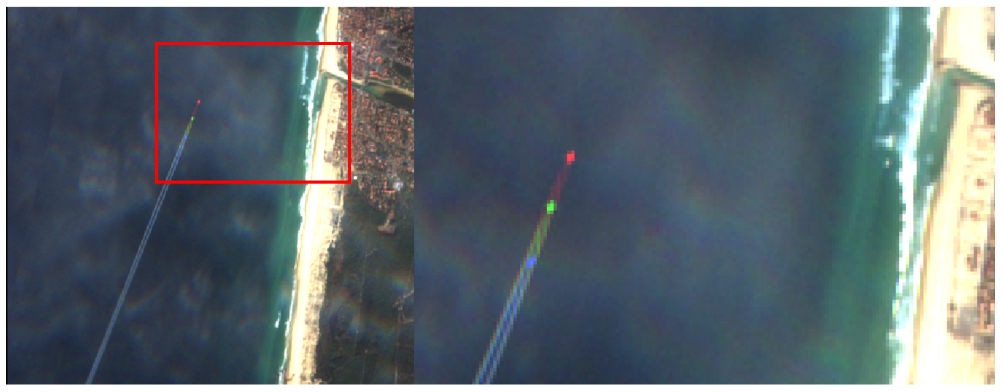
Although the Sentinel-2 products seem just a snapshot, there is underlying temporal information. The sensors collect imagery one wavelength specific-band at the time and hence, a time-lag between the different image bands exists. Such time-lag is common in optical spatial imagery and can also be found in, for example, the SPOT (max 2.04 s) and Pleiades (0.165 s between the detector bands: max 0.66 s) constellations. If we consider the bands with 10-meter resolution (red, green, blue and near-infrared), a maximum time lag of 1.005 s can be found between the blue and red band, illustrated in Figure 1. This time-lag information of Sentinel-2 has been used to determine the direction of ocean waves (a 2D-DFT has duplicate quadrants) in [19] and earlier with the SPOT constellation to estimate wave propagation through cross-correlation [16].
2.1. Radon Transform-Derived Wave Signal and Spectra
Waves can be observed from space with satellite imagery due to sunlight reflected from the sea surface (sun glitter). Satellite Sun Glitter Imagery is shown to contain valuable information to obtain wave statistics such as wave height, period and direction and even a reconstruction of the 3D surface [19]. Wave-visibility depends on several factors such as cloud coverage, satellite incident angles and wave conditions (height, period and direction). The quality/visibility of the wave pattern, and thus the ability to invert depth, differs per satellite image even for similar wave conditions. A common technique to enhance linear patterns in imagery is the Radon transform [20] (RT). Even if wave patterns are not obviously apparent and/or contain a great amount of noise, the RT distils linear features. This particular feature makes the RT a powerful tool to process imagery. RT are extensively used for tomography (for example in CT-scans) in order to reconstruct finite projections. In addition, [21,22] have shown the RT’s power in separating incident from outgoing reflected waves in the nearshore coastal zone. Here, we use the RT to extract wave signal after which we apply a 1D-DFT to find the spectral phase of the wave (per band).
In principle, the RT accentuates linear features in an image by integrating image intensity () along lines defined by angle and offset following (2):
wherein represents the Dirac delta function. represents a sinogram: the signal per direction () over the associated beam with length (). The angular limits of (2) are commonly set to . Likewise to, for example, an inverse DFT, the original input signal can be reconstructed applying an inverse RT. RT filtering means that only a limited number of angles are used for the inverse reconstruction. To isolate wave patterns, only the most energetic wave-related --pair can be used for the inverse RT.
Wave-like patterns are observed in the RT-sinogram with wave patterns in the original image. This allows for the calculation of the wave amplitude and phase per direction through a DFT (here in a discrete form). This results in a wave-number spectrum.
2.2. Waves Phase-Shift, Celerity and Depth
Imagery collected by the Sentinel-2 constellation consists of multiple bands with their specific sensing wavelength and resolution. Bands are collected one at the time with a fractional time-lag in between them. The time-lag combined with the RT-based wave number spectrum and its phase shift between bands results in the wave celerity. For each point in space, a sinogram (2) is calculated over the sub-domain. The maximum variance for all angles over is considered the propagative direction of incident waves. Over the beam with maximum variance, a DFT () is used to obtain the phase per band following:
wherein represents the DFT over the sinogram in polar space over the sub-domain around point . ℑ and ℜ respectively denote the imaginary and real part of complex numbers. For each location we can then calculate the spectral phase-shift ( in rad) between two (or more) detector bands at different times (t). Since the wave number (k) is kept fixed, a shift in spectral phase-shift represents and the celerity can be calculated:
With the derived wave celerity c and wave number k (or wavelength ) depth is found solving (1). The method as presented here selects a single, most energetic, peak in the Radon-DFT (a single wave number k) to compute the phase-shift and hence the water depth.
3. A Synthetic Deep-Water Case
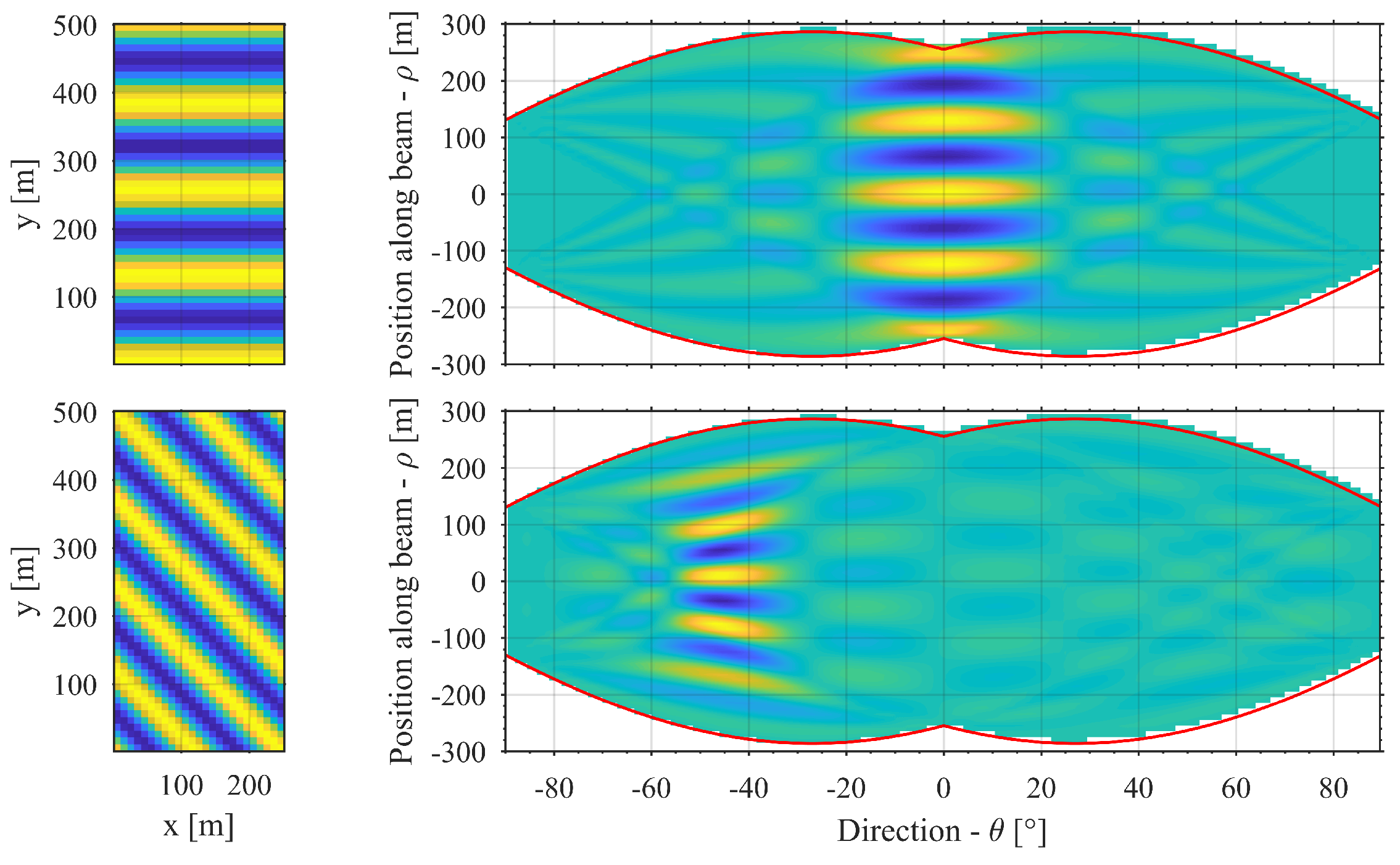
The process from a satellite image to bathymetry can be split into two main components; (1) sensing wave parameters and (2) depth-inversion. The two parts have their own associated error [12] and limits. In this section, the method steps are illustrated and the sensing capabilities of the method are scrutinized with synthetic data. Since the wave sensing principally does not depend on the relative water depth (deep, intermediate or shallow waters), it makes sense to test the sensing-method in deep water and consider pure sinusoidal waveforms. In an attempt to introduce some reality to the synthetic dataset, input-parameters are set to represent Sentinel-2 settings such as 10 m resolution and 1.005 s time-lag between two snapshots. The chosen sinusoidal has 1 m amplitude and a 9-second period which roughly correspond to the annual mean at Capbreton, France (see Section 4), resulting in two-wave patterns as shown in Figure 2. Given the wave period and considering the deep water assumption, a wavelength () of 126.36 m ( 1/m) and wave celerity (c) of 14.04 m/s can be found. This wave propagates purely in x-direction (). In addition, a second case is considered in which the wave is oblique incident () and results in a wavenumber k of 0.006 1/m and a celerity of 19.85 m/s. Here we attempt to find the appropriate wavenumber k and celerity c.
For this synthetic case, the sub-sample domain was set to 2L by 4L (252 m width × 505 m length). This is further elaborated in the discussion. Conceivably, the subsample domain size limits the appearance of the number of full wavelengths and hence the performance of the DFT (not the RT). The application of (2) to the subsample results in a sinogram, as presented in Figure 2. The upper and lower limits (red lines in Figure 2) of the beam length are computed from the center of the subsample domain. These limits were determined exclusively by the object the RT is analyzing, in this case, a rectangular sub-domain. Note that at zero degrees the limits were m to 252.5 m (total length of 505 m) and at or 90 degrees the beam stretches between m and 126 m, representing the total width of 252 m. In between , 0 and 90 degrees the sinogram limits are determined by the furthest perpendicular line of sight along the beam that senses the object (here the sub-domain). Hence, the slight increase in total beam length from zero degrees (both ways) before decreasing to the smallest beam length on the shortest side of the subdomain.
The sinograms in Figure 2 have a radial increment () of half a degree, resulting in 361 beams. A DFT is applied to every beam individually. For each rotational angle , the resolution along the RT-beam (—crossing data-points) changes and follows in case of :
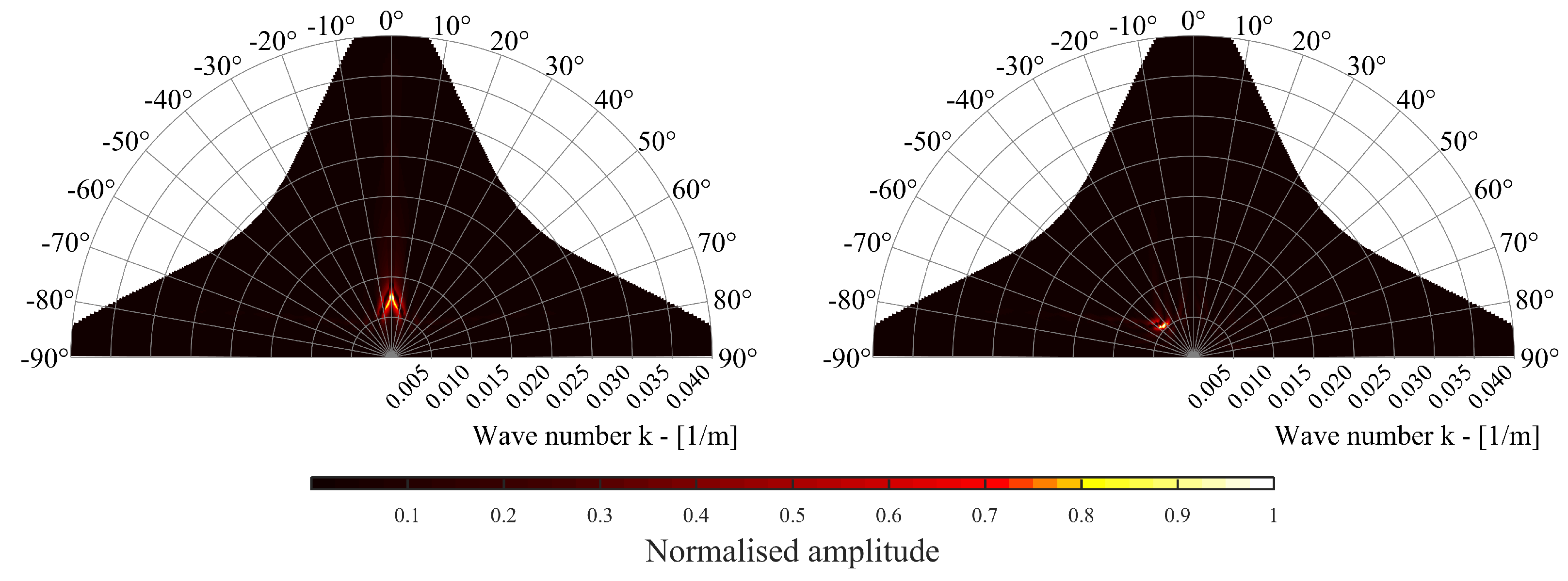
Whilst the sinogram’ resolution changes per beam, the number of sample points remains constant. Resulting RT-spectra as shown in Figure 3 have a typical cone shape: higher resolution at = , 0 or 90 degrees, results in the ability to resolve higher frequencies to a greater extent and vice versa for the diagonal. Figure 3 shows the wave-number spectra derived from the sinograms in Figure 2.
A first inspection of the energy peak in Figure 3 reveals that the incident directions correspond to the synthetic input: 0 degrees for the left plot and degrees in the right plot. The energy peaks also correspond to the appropriate wave number, respectively 0.008 [1/m] for 0 degrees case and 0.006 [1/m] for the oblique case. In both spectra, but in particular for the left plot, energy spreading is visible (in the shape of ). Along the wave track, the Radon integration solves the wave signal. As the beam rotates and the relative angle between the propagative wave and the beam direction is small, a wave signal with a longer wavelength is found (smaller wavenumber k). As this relative angle increases the energy fades out, hence the shaped energy distribution. In the case of oblique waves, the integrated energy over the wave crest perpendicular to the RT-beam (with angle ) is higher closer to the center of the sub-domain and lower towards the edges, compared to a constant crest length for 0 degrees. This effect is visible in the sinogram in Figure 2. In the lower plot ( = degrees) most of the energy is concentrated (around = 0 m, between m 100 m) while in the top plot ( = 0 degrees) the energy is more spread, between m 250 m.
The RT-DFT allows for the calculation of a spectral-phase per position on the beam, per direction. Let us impose a time lag of 1.005 s between two snapshots to the sinusoidal above and compare the phase-shift at the energy peak. For the zero degrees incident wave with a period of 9 s, the theoretical phase shift, () is 0.701 rad. The RT-DFT for the peak gives 0.701 rad shift in phase, a 0.016% offset. Given the phase shift and time-lag (), a celerity of 14.04 m/s is obtained. For the oblique waves, the estimated phase shift is 0.701 rad compared to 0.701 rad for the theoretical phase shift (0.039% offset). From the synthetic case, we can say that it is possible to estimate wave celerity accurately, in an ideal-case setting.
4. Regional Wave-Pattern and Bathymetry
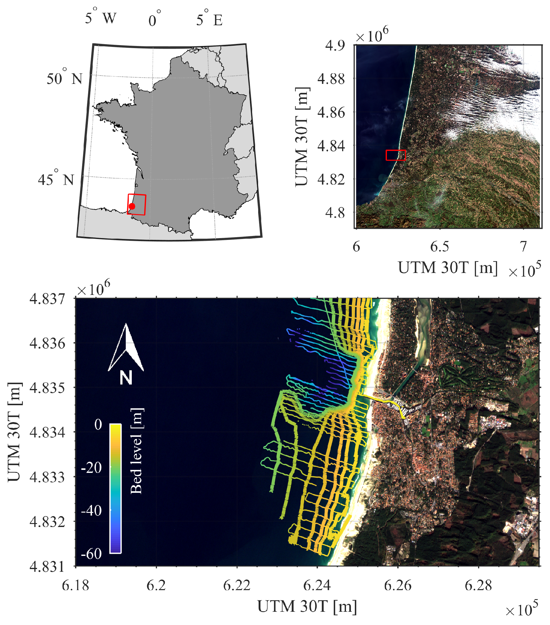
To scrutinize the method’s performance in a realistic case, it is applied to a real-world configuration. The area surrounding Capbreton in France (Figure 4) was selected considering the availability of an in-situ dataset. A field campaign was conducted from 5–18 November 2017 which was initially designed to accommodate in-situ validation of spaceborne-derived bathymetries and Digital Elevation Models (topography) using CNES’ Pleiades constellation [23,24]. The coastal zone around Capbreton is particularly suited to method-validation considering that within several kilometers one finds a variety of coastal features such as a deep-water canyon, a port entrance, hard (walls) and soft (dunes) coastal-defense structures.
During the field campaign, hydrodynamics, topography and bathymetry were measured in various ways. The hydrodynamics are captured by an acoustic doppler current profiler (ADCP) likewise waves and currents are modeled, all executed by BRGM (Pessac). The topography was measured using real-time-kinematic GPS, structure for motion (SfM) from a drone and airborne LiDAR (BRGM). The bathymetry was measured with an echo-sounder mounted on a boat and the shore-based video camera systems that deploy cBathy and the temporal method [12]. For this work, the echo-sounding measured bathymetry was considered the ground-truth. Wave conditions were of special interest as incident waves might influence the space-borne bathymetry inversion quality [12]. Here, the two closest nearshore wave buoys in the Bay of Biscay were used to obtain wave data (Wave buoy number 62066 – Anglet and number 62064 – Arcachon). During the field campaign, the dominant wave conditions were quite energetic. Wave height conditions ranged between 0.7 and 4.4 m with a mean significant wave height of 2.22 m. The maximum wave height had an associated period of 15.4 s. The maximum wave period went up to 18.4 s with an associated wave height of 1.2 m. The wave direction was relatively constant considering a mean direction 307.2 degrees ± 7.56 degrees.
In this paper we test RT-based wave pattern extraction on 10 × 10 m resolution Sentinel-2 imagery [25] covering the region surrounding Capbreton\—\Sentinel-2 relative orbit 94, tile 30TXP—on two dates: (1) 2 days after the end field campaign on 20 November 2017 and (2) preferable wave conditions (30 March 2018). The bathymetry is only derived for the latter to demonstrate the methods’ performance.
4.1. Parameter Settings for the rt Method
Few parameter settings were required to apply the RT for wave pattern extraction and wave-number spectra, and these were only limited to the spatial domain. An RT-filter was applied every 50 m in x and y direction, ( and 50 m), in other words, the depth estimation results have a horizontal resolution of 50 m. The windowing sub-domain for this real-world case is currently set to 30 × 20 pixels which practically relates to 300 × 200 m and an amplification factor () is applied as a function of the distance (D in km) from the coastline . The size of the sub-sample domain is in a similar order compared to [15,17,18], and relates mostly to the stochasticity of the sub-sampled wave pattern. In other words, to apply typical methods such a wavelet or DFT analysis, more than a single wavelength should be sub-sampled, the same holds here.
For the RT-based phase-shift derived celerity, limits are imposed. The estimated celerity should be greater than zero and cannot exceed the deep water limit related to a user-defined maximum wave period. Here the cut-off wave period is 18 s, which relates to 28.1 m/s. This should be considered quite a generous upper limit, as these waves are not expected to travel with these celerities in the coastal zone. In addition to the minimum wave celerity threshold, sensed depth can only be positive (before it is referenced to a vertical datum).
4.2. Wave Extraction: Illustration
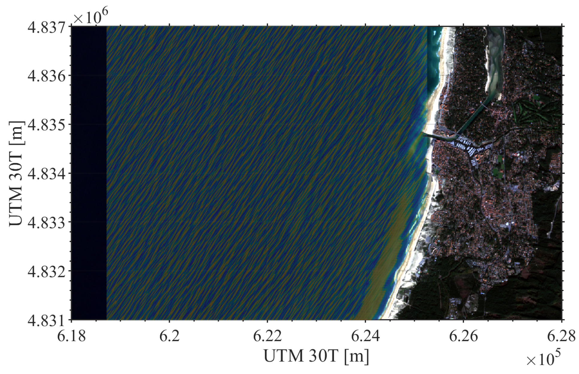
To show the power of RT-filtering we apply it on Sentinel-2 imagery collected at Capbreton on 20 November 2017. A wave pattern is not apparent in the raw level-2 Sentinel-2 imagery. The two closest wave buoys in the Bay of Biscay (buoy-ID 62066 and 62064—Global GlobWave database) measured an average significant wave height of 0.58 to 0.66 m, an average peak period of 11.72 to 11.76 s and a peak-associated wave direction of 274 to 326 degrees. These relative calm wave conditions result in an imperceptible wave pattern in the satellite imagery. Often these images are discarded for further analysis but let’s consider this image as a nice example-case for RT filtering. The RT filtering as in phase I of the methodology is applied per sub-domain and normalized over the full domain. Figure 5 shows the filtered result over approximately 30 km.
The filtered image clearly shows the incident wave pattern in the appropriate direction. In addition, secondary wave-like patterns are apparent such as the satellite sensor direction (lines with 290 degrees angle). This seems to be linked to the signal to noise ratio, as the wave signal is imperceptible and the sensing leaves a trace of a similar order of magnitude the RT also amplifies this artifact. At the coast, particularly South of the harbor entrance, larger, non-physical, intensities are observed (wide yellow band). This is due to the fact that the RT sees the coast as the most energetic linear feature in that sub-domain and the results are maxed-out.
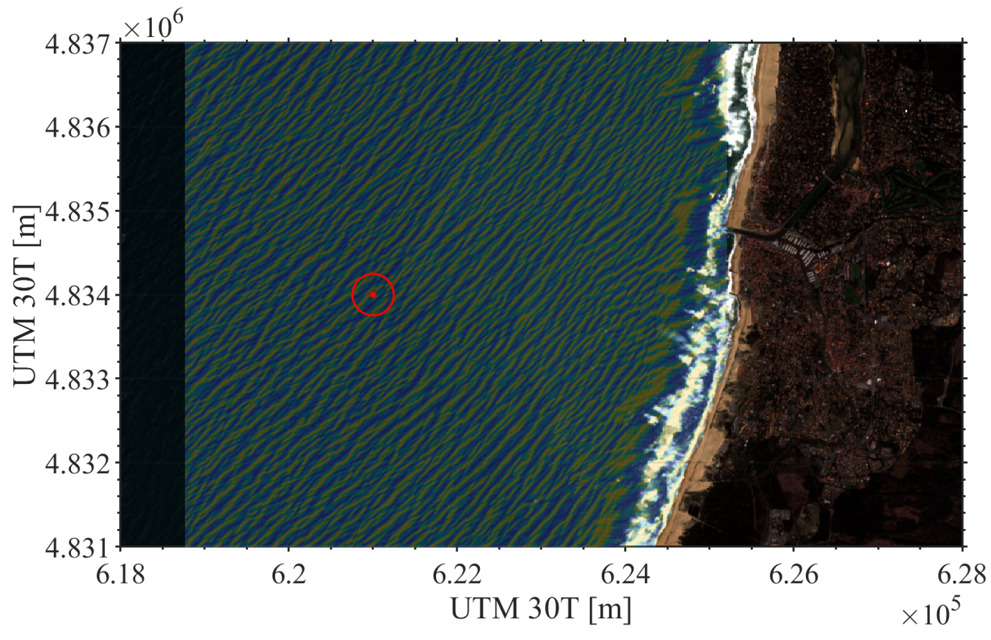
In case incident waves are steeper, greater wave height and similar period, wave patterns are easier to observe from the satellite imagery. Figure 6 shows RT results for the wave pattern extraction on 30 March 2018 under wave conditions of 3.26 to 3.3 m average significant wave height, an average peak wave period between 12.69 and 12.79 s and an incident wave-angle between 280 to 309 degrees. Also, the incident swell was cleaner and had less directional spread (10–20 degrees) on 30 March 2018 in comparison to 20 November 2017 (13–30 degrees). The wave pattern was significantly more distinctive in comparison to Figure 5. For example, refraction patterns around the harbor entrance were visible.
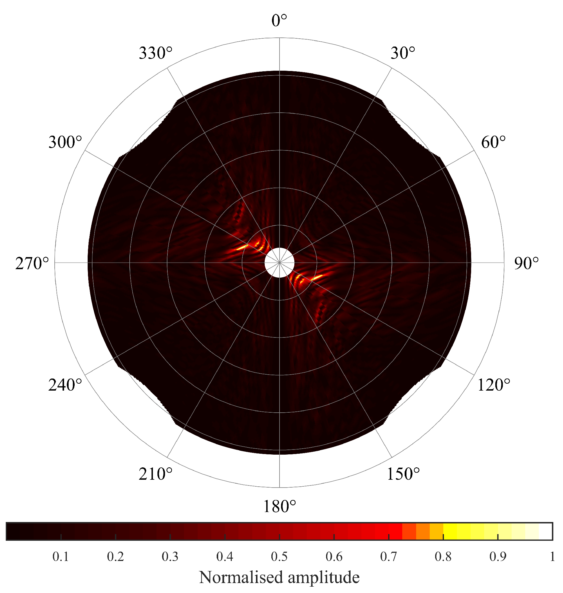
For the wave pattern in Figure 6, unfiltered (all directions), a RT-based spectrum can be derived for every location (). Figure 7 shows an example of such spectrum for point x = 621,000 m and y = 4,834,000 m, roughly in the middle of the domain as indicated by the red circle in Figure 6. The spectral coloring in Figure 7 relates to the normalized amplitude. This RT wavenumber spectrum confirms shows similar wave direction and spreading as the offshore wave buoy. Figure 7 also indicates the RT-related energy spreading, likewise to the synthetic spectra.
4.3. Wave Number and Depth Estimation
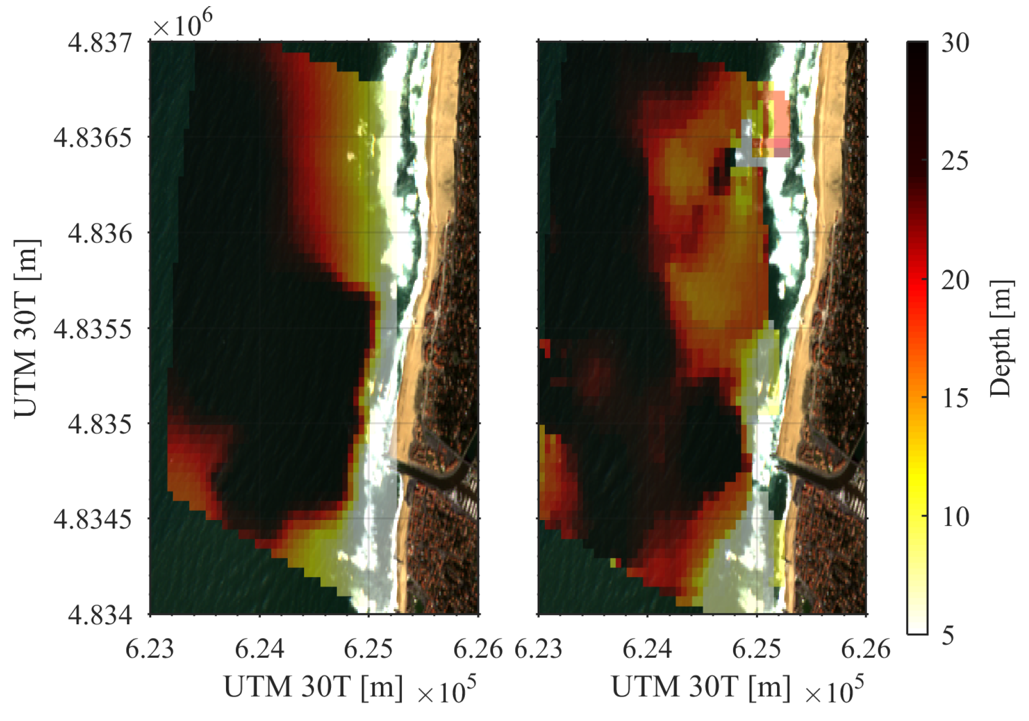
Several distinct energy concentrations are apparent in the wave-number spectrum around the 300 degrees spoke for wave numbers around 0.005 m. The derived spectrum confirms what the wave buoy data told us in the sections above. Which energy peak to use for the depth inversion for each spectrum is not trivial. Here, the current set-up takes the direction from the variance peak in the sinogram. For the wave number the 99% interval is calculated, so the 1% most energetic points, from the normalized amplitude spectrum. For the most energetic 1% wavenumber k is computed and used to calculate the phase-shift. Figure 8 shows the measured depth and depth derived from Sentinel-2 imagery acquired on 30 March 2018. Bear in mind, these are tide-corrected depths (tidal elevation = m). Here, depths are estimated over the same domain as the field-campaign covered.
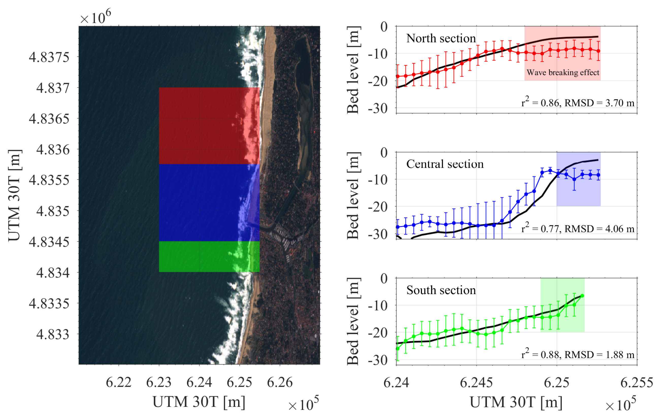
The measured and estimated depth shows comparable morphological features. The deep-water canyon (300 m depth close to shore) in front of the harbor is recognizable. Features like these are often lacking in state-of-the-art applications because they are relatively hard to resolve. Between the survey and estimation, a correlation coefficient of 0.82 and RMS difference of 2.58 m is found for measured depths up to 30 m. The correlation coefficient shows that the estimated morphological features have a physical meaning and represent reality. Figure 9 presents sectioned profiles: North, central (with the deep-water canyon) and the South section. In the North, one can see that the depth is well estimated until the sub-tiles hit the white water due to wave breaking. In the canyon section, we do estimate the canyon outline but we underestimate the canyon’ slope nearshore. This offset in the vicinity of the canyon can be explained by complex wave attenuation on the canyon banks as the waves make a quick transition between deep-water to shallow water: multiple spectral peaks disperse the computed phase shift. This could be solved by introducing depth estimation over multiple wave numbers (not included in the current version). In the Southern section, the waves were less affected by the deepwater canyon and the wave breaking zone is less wide, the depth estimation technique does quite well. These results, the presence of the canyon and adequate estimation of the shallowest depths, show the potential of this novel estimation of the wave-phase shift, and celerity in polar (RT) space.
5. Discussion
The results show that wave patterns can be extracted by a local application of the RT for two different wave conditions and depth can be estimated. Wave-enhancement is an intrinsic characteristic of the RT while depth inversion from the RT spectra depends on the physical and sensing conditions. What are the limitations, in particular at other different coastal wave environments? To a certain degree, all coastal zones host waves passing through. Depth inversion depends, in the first instance, on the wave period/length and image resolution while the wave observability greatly depends on the relative angles between incident waves, satellite view angle and position of the sun [26] but also wave characteristics such as wave steepness (). Here, we focus on the methodological aspect imposed limits by the image resolution.
5.1. Required Sensing Resolution
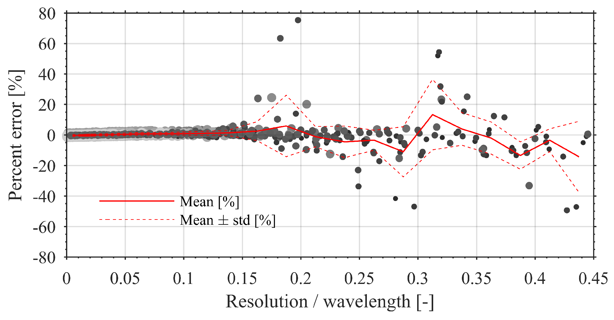
The image resolution predominantly determines whether one can see waves or not; this holds for all imagery from shore-based video, airborne systems to space-borne optical and radar imagery. One could argue that at the very least 2 points over a full wavelength (Nyquist criterion) are required to start recognizing a waveform. At the same time, waveforms are asymptotically better visible than the more points per wavelength. In order to isolate and scrutinize the methodology’s limits, synthetic data is used. Let’s consider a synthetic dataset representing an image-resolution range between 0.5 m (Pleiades) and 100 m (THIR bands of NASA’ Landsat-8) in combination with a set of wavelengths related to their offshore period (from 4 to 20 s with half a second interval). This results in 33 different wave periods and 29 resolutions, hence a total of 957 configurations. Perhaps it is stating the obvious, but the most coarse resolution will not be sufficient to resolve the shortest waves and are then neglected (resolution > 0.5). For each wave and resolution pair, the phase-shift difference between the theoretical and estimated shift is determined. Figure 10 shows the percent error as a function of the resolution/.
Figure 10 shows that independently of the wave period/length the percent error starts to increase and vary significantly after an image resolution over the wavelength-ratio of 0.15. A careful look at the data reveals that for ratios near zero to 0.13 the percent error is smaller than 1% and the standard deviation is smaller than 1.5%. Beyond the 0.17 ratio, the mean percent error varies between 4.25% and with standard deviations up to 23.3%. The 0.13 and 0.15 ratios mean that 6.67 (0.15) to 7.69 (0.13) points are required on the full wavelength to resolve the wave phase shift appropriately. For Sentinel-2’s best resolution (10 m) this means 7–8 pixels, and thus, wavelengths smaller than 70–80 m are not sufficiently resolved to estimate the phase shift. From this analysis, a required sensing resolution can be determined per wave period or wavelength, as shown in Figure 11.
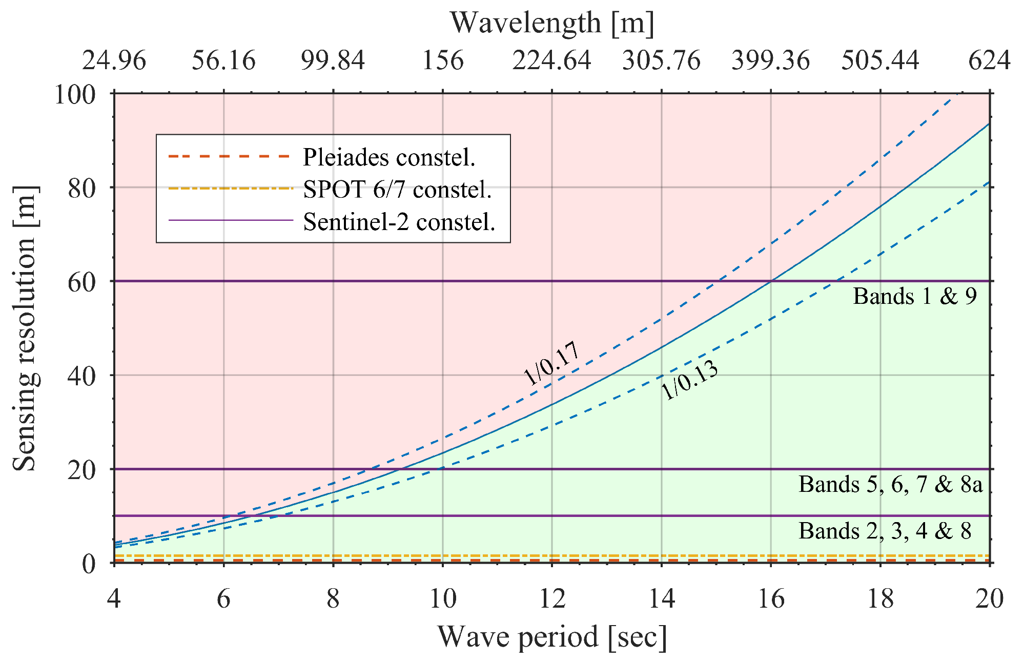
The blue solid line in Figure 11 indicates the 0.15 ratio between resolution and wavelength. The right of this line means that the resolution is sufficient to resolve the wave phase shift with the current method (green area), and the vice versa for the left-hand side of the blue line (red area). With the Sentinel-2 constellation, one should typically be able to resolve waves with a period equal to or greater than 7 s. This represents the offshore period here, in the coastal zone, nearshore hydrodynamic processes, such as shoaling, shift this boundary upwards. In addition to the Sentinel-2 constellation, the Pleiades (0.5 m) and SPOT 6/7 (1.5 m) are represented by a horizontal line in Figure 11. Both constellations do not have limitation to observe the smallest wind-wavelengths and periods. For example, for the lower wind-wave period, let’s say 3 s, the Pleiades constellation has already 14 points over a full offshore wavelength. However, the limitation for the Pleiades constellation is the interval between images, either 0.146 s between image-bands (as used here) or 8 s between individual snapshots. Hence waves with a period smaller than 8 s cannot be resolved [26].
5.2. Sentinel-2 Bands Resolution Augmentation
Besides Sentinel-2’ highest 10 m resolution bands (RGB+NIR), lower resolution (20 m and 60 m) visible bands are acquired [27]. Presuming that all these bands observe a similar wave pattern (which depends on the detector-wavelength). The time-lag between the detector-bands and the first band (Blue–band-2) increases from 0.264 to 2.586 s for the last band (band-9 with 60 m resolution) as shown in Table 1. To observe wave propagation one could argue that the resolution of the imagery should be smaller than the distance covered by the wave over t. The larger the t, the better observable wave propagation should be. For example, considering the 60 m Sentinel-2 resolution, waves have to travel 60 m in 2.586 s requiring a celerity of 23.2 m/s, which is quite fast for free surface waves in the nearshore. For the 10 m (1.005 s) and 20 m (2.055 s) resolution bands, the optimum is respectively 9.95 m/s and 9.73 m/s. Furthermore, according to Figure 11, lower resolution images with 60 m would only be sufficient to resolve celerity for waves with a period of 16 s or longer. Stepping up to the higher-resolution 20 m Sentinel-2 bands waves with a 9.25 s period can be resolved.
A multi-band/multi-resolution combination to compute the celerity is a possibility. [16] uses two bands with different resolution from SPOT-5 for a sub-pixel cross-correlation. However, this approach requires significant computational power. As mentioned before, the RT is used in image processing to augment image resolution. The RT sinogram is interpolated and subsequently used in the inverse RT, and so, augmenting the image resolution. Let us focus on Sentinel-2 band 8a which has 20 m resolution and the largest time-lag with respect to band 2 (Table 1). The time-lag between Band-2 (the first band—Figure 6) and the 20 m resolution bands range between 1.269 s to 2.055 s making them very useful in the phase-shift analysis if augmented to 10 m resolution.
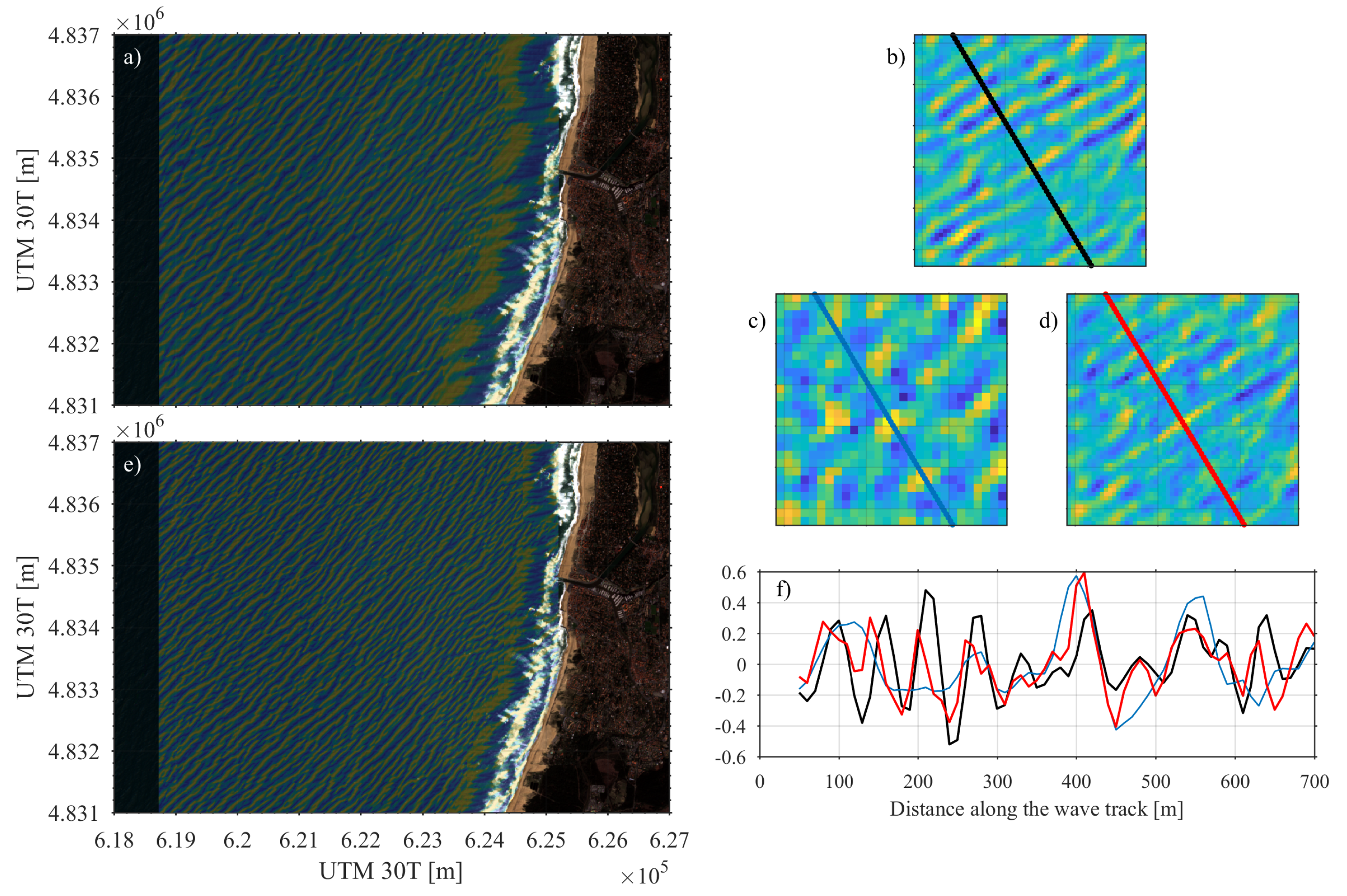
From Figure 12 one can see that the 20 m resolution resembles the incident wave pattern at large, for the longer wavelengths. Smaller wave features, present in Figure 6 are not visible and particularly at the coast the wave pattern is not well resolved. The RT-augmented wave pattern in Figure 12b contains smaller wave patterns, like the original 10 m resolution wave pattern in Figure 6. At the coast, the refraction pattern around the harbor is clearly visible now. Focussing on the sub-sampled wave patterns in Figure 12b–d, the effect of the augmentation is even more apparent. The ocean wave pattern in Figure 12c is incomparable to that in Figure 12b. Using correlation methods to find the celerity would be a challenge here. However, as in Figure 12d in case the Radon-based augmentation is applied, similar (shifted) wave patterns become visible. Figure 12f highlights this in even greater detail. For example, between 150–300, hardly any wave signal is visible in the blue line (B05-original) while the red line (B05-augmented), represents a similar wave pattern as found with the 10 m resolution band B02.
The RT-augmented wave pattern augmentation allows the 20 m resolution bands to be used alongside the 10 m bands, so that wave phase can be computed over bands 2 to 8a. Discarding band 3 and 8 (time-lag < 0.55 s), a wave phase-shift can then be computed between detector band-2 and the five other bands (B4, B5, B6, B7, B8a). Conceivably, more usable frames will improve the method’ robustness. Noteworthy, this technique can also be applied to augment 10 m imagery to higher resolutions. If so, to a certain degree this augmentation diminishes the minimally required wave period to sense the wave celerity. This first application shows promising but the limits of Radon-based augmentation must be explored as well as the use of multiple bands to determine celerity, and a large variety of wave conditions (likewise for the depth estimation).
6. Conclusions
In this work, an RT-based wave-pattern extraction, augmentation and depth inversion method are presented. Wave patterns are extracted by applying an RT and subsequent angle filtering to Sentinel-2 imagery so that the wave signal contains the most-dominant wave directions. Depth is derived exploiting the time-lag between detector-bands. The wave-phase per band, and after the phase shift, is obtained by applying a DFT to the RT sinogram over a local sub-domain. Depths are derived with a good correlation of 0.82 and 2.58 m RMS error over the surveyed domain. These results are beyond the expectations considering the challenging environment including a deep-water canyon and its effect on surrounding wave patterns. In terms of international admiralty standard [28] the measurements could be qualified as level C (up to 30 m). Besides physical limits of the linear dispersion relation, image resolution limits adequate observation of the wave celerity. This method is shown to work stably for waves with a period larger than 6.5 s. In addition to the wave pattern extraction and depth derivation, the RT can be used to augment image resolution. 20 m resolution image bands, from Sentinel-2, are augmented to match the 10 m resolution bands allowing those four extra bands to be used in the depth estimation method, with time-lags ranging between 1.005 s to 2.055 s.
Author Contributions
Conceptualization, E.W.J.B. and R.A.; methodology, E.W.J.B.; validation, E.W.J.B.; resources, E.W.J.B., R.A. and P.M.; data curation, E.W.J.B. and R.A.; writing—original draft preparation, E.W.J.B.; writing—review and editing, E.W.J.B., R.A. and P.M.; visualization, E.W.J.B.; supervision, R.A. and P.M.
Funding
E. Bergsma was partly funded by IRD (Institut de Recherche pour le Développement) and is currently part of the CNES post-doctoral fellowship-program to develop this work. The authors would like to thank CNRS/LEGOS for funding the COMBI-project that initiated this work and provided the in-situ data.
Acknowledgments
We would like to thank the French National Space Agency (CNES) for facilitating fruitful discussions between their Sentinel team, support and scientists. Evidently, this work would not be possible without ESA’s Earth Observation and EU’s Copernicus programme. We are grateful to ESA and EU for their efforts to make satellite imagery (optical and radar) more accessible to the public. The authors would to thank Luis Pedro Almeida and Paulo Baganha Baptista for the execution of the bathymetry survey and in cooperation with, and amazing support from D. Legros.
Conflicts of Interest
The authors declare no conflict of interest. The funders had no role in the design of the study; in the collection, analyses, or interpretation of data; in the writing of the manuscript, or in the decision to publish the results.
References
- Vitousek, S.; Barnard, P.L.; Fletcher, C.H.; Frazer, N.; Curt, D.; Storlazzi, L.E. Doubling of coastal flooding frequency within decades due to sea-level rise. Sci. Rep. 2017, 7, 1399. [Google Scholar] [CrossRef] [PubMed]
- Vousdoukas, M.; Mentaschi, L.; Voukouvalas, E.; Feyen, L. Climatic and socioeconomic controls on coastal flooding impacts in Europe. Nat. Clim. Chang. 2018, 8, 776–780. [Google Scholar] [CrossRef]
- Cazenave, A.; Le Cozannet, G.; Benveniste, J.; Woodworth, P.; Champollion, N. Monitoring coastal zone changes from space. EOS 2017, 98. Available online: https://eos.org/opinions/monitoring-coastal-zone-changes-from-space (accessed on 5 July 2019). [CrossRef]
- Li, J.; Roy, D.P. A Global Analysis of Sentinel-2A, Sentinel-2B and Landsat-8 Data Revisit Intervals and Implications for Terrestrial Monitoring. Remote Sens. 2017, 9, 902–919. [Google Scholar]
- Lyzenga, D. Passive remote sensing techniques for mapping water depth and bottom features. Appl. Opt. 2018, 17, 379–383. [Google Scholar] [CrossRef] [PubMed]
- Holman, R.A.; Plant, N.; Holland, T. cBathy: A Robust Algorithm For Estimating Nearshore Bathymetry. J. Geophys. Res. Oceans 2013, 118, 2595–2609. [Google Scholar] [CrossRef]
- Bergsma, E.W.J.; Conley, D.C.; Davidson, M.A.; O’Hare, T.J. Video-Based Nearshore Bathymetry Estimation in Macro-Tidal Environments. Mar. Geol. 2016, 374, 31–41. [Google Scholar] [CrossRef]
- Brodie, K.; Palmsten, M.; Hesser, T.; Dickhudt, P.; Raubenheimer, B.; Ladner, H.; Elgar, S. Evaluation of video-based linear depth inversion performance and applications using altimeters and hydrographic surveys in a wide range of environmental conditions. Coast. Eng. 2018, 136, 147–160. [Google Scholar] [CrossRef] [Green Version]
- Stockdon, H.F.; Holman, R.A. Estimation of wave phase speed and nearshore bathymetry from video imagery. J. Geophys. Res. 2000, 105, 22015–22033. [Google Scholar] [CrossRef]
- Plant, N.G.; Holland, K.T.; Haller, M.C. Ocean Wavenumber Estimation from Wave-Resolving Time Series Imagery. IEEE Trans. Geosci. Remote Sens. 2008, 46, 2644–2658. [Google Scholar] [CrossRef]
- Almar, R.; Bonneton, P.; Senechal, N.; Roelvink, D. Wave Celerity from Video Imaging: A new method. In Proceedings of the 31st International Conference Coastal Engineering, Hamburg, Germany, 31 August–5 September 2008; pp. 1–14. [Google Scholar]
- Bergsma, E.W.J.; Almar, R. Video-based depth inversion techniques, a method comparison with synthetic cases. Coast. Eng. 2018, 138, 199–209. [Google Scholar] [CrossRef]
- Williams, W.W. The determineation of Gradients on enemy-held beaches. Geogr. J. 1946, 109, 76–90. [Google Scholar] [CrossRef]
- Abileah, R. Mapping shallow water depth from satellite. In Proceedings of the ASPRS Annual Conference, Reno, NV, USA, 1 May 2006. [Google Scholar]
- Poupardin, A.; Idier, D.; de Michele, M.; Raucoules, D. Water Depth Inversion From a Single SPOT-5 Dataset. IEEE Trans. Geosci. Remote Sens. 2016, 119, 2329–2342. [Google Scholar] [CrossRef]
- de Michele, M.; Leprince, S.; Thiébot, J.; Raucoules, D.; Binet, R. Direct Measurement of Ocean Waves Velocity Field from a Single SPOT-5 Dataset. Remote Sens. Environ. 2012, 119, 266–271. [Google Scholar] [CrossRef]
- Poupardin, A.; de Michele, M.; Raucoules, D.; Idier, D. Water depth inversion from satellite dataset. In Proceedings of the 2014 IEEE Geoscience and Remote Sensing Symposium, Quebec City, QC, Canada, 13–18 July 2014; pp. 2277–2280. [Google Scholar]
- Danilo, C.; Farid, M. Wave period and coastal bathymetry using wave propagation on optical images. IEEE Trans. Geosci. Remote Sens. 2016, 54, 6307–6319. [Google Scholar] [CrossRef]
- Kudryavtsev, V.; Yurovskaya, M.; Chapron, B.; Collard, F.; Donlon, C. Sun glitter imagery of ocean surface waves. Part 1: Directional spectrum retrieval and validation. J. Geophys. Res. Oceans 2017, 122, 1369–1383. [Google Scholar] [CrossRef] [Green Version]
- Radon, J. Ufiber die bestimmung von funktionen durch ihre integral-werte langs gewisser mannigfaltigkeiten. Sachs. Akad. Der Wiss. Leipz. Math-Phys 1917, 62, 262–267. [Google Scholar]
- Almar, R.; Michallet, H.; Cienfuegos, R.; Bonneton, P.; Tissier, M.; Ruessink, G. On the use of the Radon Transform in studying nearshore wave dynamics. Coast. Eng. 2014, 92, 24–30. [Google Scholar] [CrossRef]
- Martins, K.; Blenkinsopp, C.E.; Almar, R.; Zang, J. The influence of swash-based reflection on surf zone hydrodynamics: A wave-by-wave approach. Coast. Eng. 2017, 122, 27–43. [Google Scholar] [CrossRef]
- Berthier, E.; Vincent, C.; Magnússon, E.; Gunnlaugsson, A.; Pitte, P.; Meur, E.L.; Masiokas, M.; Ruiz, L.; Pálsson, F.; Belart, J.M.C.; et al. Glacier topography and elevation changes derived from Pléiades sub-meter stereo images. Cryosphere 2014, 8, 2275–2291. [Google Scholar] [CrossRef]
- Almeida, L.P.; Almar, R.; Bergsma, E.W.J.; Berthier, E.; Baptista, P.; Garel, E.; Dada, O.; Alves, B. High resolution coastal topography from satellite stereo imagery. Remote Sens. 2019, 11, 590. [Google Scholar] [CrossRef]
- Drusch, M.; Bello, U.D.; Carlier, S.; Colin, O.; Fernandez, V.; Gascon, F.; Hoersch, B.; Isola, C.; Laberinti, P.; Martimort, P.; et al. Sentinel-2: ESA’s Optical High-Resolution Mission for GMES Operational Services. Remote Sens. Environ. 2012, 120, 25–36. [Google Scholar] [CrossRef]
- Almar, R.; Bergsma, E.W.J.; Maisongrande, P.; Almeida, L.P. Coastal bathymetry from optical submetric satellite video sequence: A showcase with Pleiades persistent mode. Remote Sens. Environ. 2019, 231, 111263. [Google Scholar] [CrossRef]
- SUHET. Sentinel-2 User Handbook; ESA-ESTEC: Noordwijk, The Netherlands, 2015. [Google Scholar]
- Admiralty Charts: Zones of Confidence (ZOC) Table. Available online: https://www.admiralty.co.uk/AdmiraltyDownloadMedia/Blog/CATZOC (accessed on 5 August 2019).
Figure 1.
Illustration of the time-lag between detector bands B02 (blue), B03 (green) and B04 (red) by the different colors of the flying airplane at Capbreton, France. The time-lag between each band is 0.527 s.
Figure 1.
Illustration of the time-lag between detector bands B02 (blue), B03 (green) and B04 (red) by the different colors of the flying airplane at Capbreton, France. The time-lag between each band is 0.527 s.

Figure 2.
Radon transform sinograms for the synthetic datasets containing (1) a shore normal wave (0 degrees) and (2) an oblique example where = . The red lines indicate the sinograms limits along the beam length.
Figure 2.
Radon transform sinograms for the synthetic datasets containing (1) a shore normal wave (0 degrees) and (2) an oblique example where = . The red lines indicate the sinograms limits along the beam length.

Figure 3.
Normalized Radon-discrete fast-Fourier transform (DFT) wave number spectra for a wave in shore normal direction at the top and oblique ( deg) incident wave in the bottom. The wave number range is between 0 and 0.04 [1/m] with 0.001 [1/m] resolution, the circular bands indicate 0.005 [1/m] intervals. The direction ranges from to 90 with a of 0.5 degree, the spokes represent a 10-degree interval.

Figure 4.
Location of Capbreton in South–West France. The top-left overview shows part of Western Europe in which France is highlighted as the darker grey area (coordinate system WGS84). The red dot represents Capbreton and the box around the dot represents Sentinel-2 tile 30TXP projected on the UTM-zone 30T (Universal Transverse Mercator) . The tiled Sentinel-2 image is presented at the top-right (image taken on 20 November 2017). The red box in the top-right figure highlights the zoomed-in area of the bottom plot. The small dots (mainly on cross shore arrays) represent the echo-sounder measured depths. The thicker predominantly alongshore lines represent the depth isocontours. The deep-water canyon (dark blue dots) is evident close to shore, West–Northwest of the harbour entrance. The echo-sounder was realistically capable of measuring from the shallowest as the boat would go until 60–70 m water depth.

Figure 5.
Radon-filtered wave pattern (normalized) from Sentinel-2 imagery collected on 20 November 2017.
Figure 5.
Radon-filtered wave pattern (normalized) from Sentinel-2 imagery collected on 20 November 2017.

Figure 6.
Radon-filtered wave pattern (normalized) from Sentinel-2 imagery collected on 30 March 2018. The red circle indicates the position related to the Radon-derived wave spectrum.
Figure 6.
Radon-filtered wave pattern (normalized) from Sentinel-2 imagery collected on 30 March 2018. The red circle indicates the position related to the Radon-derived wave spectrum.

Figure 7.
Full Radon spectrum derived from Sentinel-2 imagery that was sensed on 30 March 2018. The circular bands follow the same increment (0.005 [1/m]) as Figure 3 but the range is limited to 0.03 [1/m]. The off-shore wave-period range in this spectrum was 5 s (0.0256 [1/m]) to 18 s (0.002 [1/m]).

Figure 8.
Measured (left) and Sentinel-2 estimated (right) water depths in the vicinity of the Capbreton harbour. The measured bathymetry is interpolated on the depth estimation locations. This highly complex bathymetry, in particular the contours of the deep-water channel and nearshore zone South of the harbour entrance show similarities.

Figure 9.
Sectioned profiles considering North of the canyon (red), a central part including the deep water canyon (blue) and South of the canyon (green). The black line illustrates the measured profile while the colors are the estimated profiles using the RT-based depth estimation.
Figure 9.
Sectioned profiles considering North of the canyon (red), a central part including the deep water canyon (blue) and South of the canyon (green). The black line illustrates the measured profile while the colors are the estimated profiles using the RT-based depth estimation.

Figure 10.
Percent error per image resolution () over wavelength (). The solid red line represents the mean per bin 0.025 [-] (Res/) and the dotted red lines represent the associated standard deviation (). The color and size of the scatter relates to the wave period: the larger the period, the bigger and lighter the dots.

Figure 11.
Sensing resolution as a function of wave period/length. The solid blue line represents the resolution’s limit to resolve an associated deep-water wave period/length. The green area indicates sufficient resolution while the opposite is true for the red area. The purple lines (Sentinel-2 constellation) are plotted for bands 1 to 9 with 10, 20 and 60 m resolution.

Figure 12.
Augmentation of Sentinel-2’ mid-resolution bands (20 m) to the high-resolution (10 m). (a) shows the sensed 20 m resolution wave pattern (normalized) derived from detector-band 5 and (e) shows the augmented wave pattern (normalized) using a localized Radon transform and interpolation of the local Radon-sinogram. (b–d,f) show the effect on the obtained wave signal. (b) is a subsample of the B02 band (10 m resolution), (c) represents the sensed subsample of band B05 (20 m resolution) and (d) is the radon-augmented version (10 m resolution). (f) presents the spatial wave-signal along wave-track following the color-coding as in (b–d).


Table 1.
Detector bands Sentinel-2: visible and near-infrared [27].
Table 1.
Detector bands Sentinel-2: visible and near-infrared [27].
| Band | t [Sec] | Av. Wavelength (S2A/S2B) [nm] | Resolution [m] |
|---|---|---|---|
| 2 | 0 | 492.3 | 10 |
| 8 | 0.264 | 832.9 | 10 |
| 3 | 0.527 | 559.4 | 10 |
| 4 | 1.005 | 664.8 | 10 |
| 5 | 1.269 | 704.0 | 20 |
| 6 | 1.525 | 739.8 | 20 |
| 7 | 1.790 | 781.3 | 20 |
| 8a | 2.055 | 864.4 | 20 |
| 1 | 2.314 | 442.5 | 60 |
| 9 | 2.586 | 944.1 | 60 |
© 2019 by the authors. Licensee MDPI, Basel, Switzerland. This article is an open access article distributed under the terms and conditions of the Creative Commons Attribution (CC BY) license (http://creativecommons.org/licenses/by/4.0/).
Share and Cite
MDPI and ACS Style
Bergsma, E.W.J.; Almar, R.; Maisongrande, P. Radon-Augmented Sentinel-2 Satellite Imagery to Derive Wave-Patterns and Regional Bathymetry. Remote Sens. 2019, 11, 1918. https://0-doi-org.brum.beds.ac.uk/10.3390/rs11161918
AMA Style
Bergsma EWJ, Almar R, Maisongrande P. Radon-Augmented Sentinel-2 Satellite Imagery to Derive Wave-Patterns and Regional Bathymetry. Remote Sensing. 2019; 11(16):1918. https://0-doi-org.brum.beds.ac.uk/10.3390/rs11161918
Chicago/Turabian StyleBergsma, Erwin W. J., Rafael Almar, and Philippe Maisongrande. 2019. "Radon-Augmented Sentinel-2 Satellite Imagery to Derive Wave-Patterns and Regional Bathymetry" Remote Sensing 11, no. 16: 1918. https://0-doi-org.brum.beds.ac.uk/10.3390/rs11161918
Note that from the first issue of 2016, this journal uses article numbers instead of page numbers. See further details here.