Learnable Gated Convolutional Neural Network for Semantic Segmentation in Remote-Sensing Images

 ,
,
Abstract
:
1. Introduction
2. Related Works
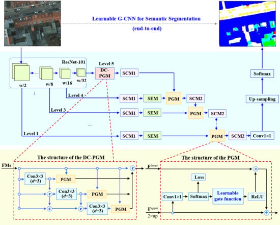
3. Method
3.1. Parameterized Gate Module
3.2. Densely Connected Pgm
3.3. L-GCNN Neural Architecture
3.4. Training and Inference
| Algorithm 1: Training algorithm for the proposed L-GCNN. |
| Input: Training samples composed of images and their corresponding segmented ground truth labels , regularization parameters and , learning rate and maximum number of iterations T. Output: Network parameters in of L-GCNN.
|
4. Experiments
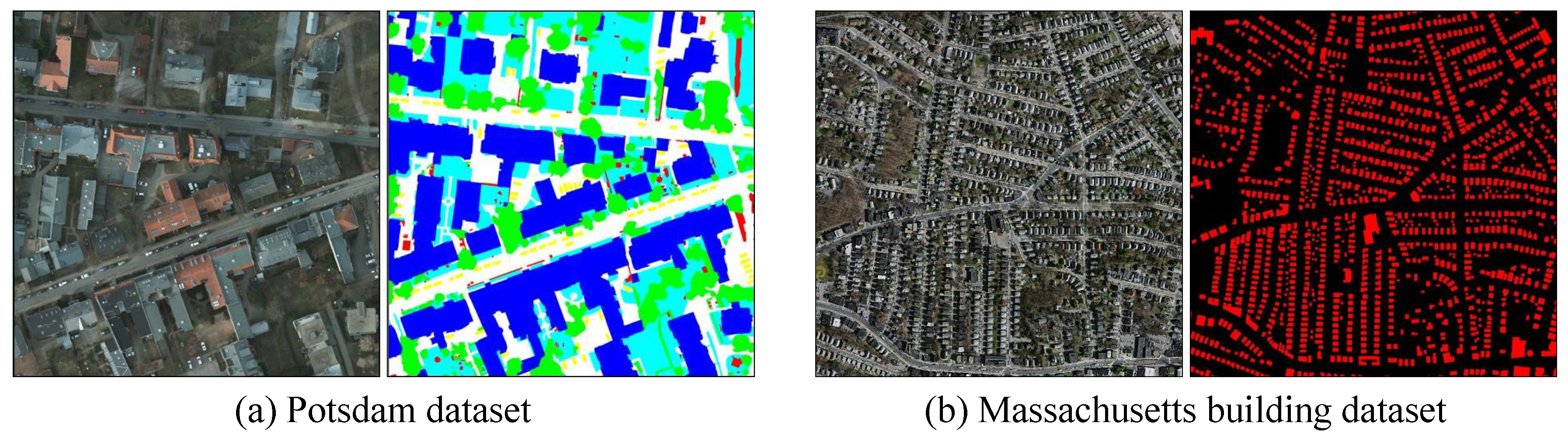
4.1. Data Description
4.2. Evaluation Metrics
4.3. Compared Methods and Experiment Settings
- FCN: a seminal work proposed by Long et al. [24] for semantic segmentation. Currently, it is usually taken as the baseline for comparison. Three versions of FCN models, FCN-32s, FCN-16s and FCN-8s, are available for public use. From them, the FCN-8s model with fine edge segmentation preserving was employed for comparison.
- SegNet: This model was actually developed on the FCN framework by employing pooling indices recorded in the encoder to fulfil nonlinear upsampling in the decoder [26]. It is now taken as a fundamental structure for comparative evaluation on semantic segmentation.
- RefineNet: It is an approach for natural-image segmentation that takes ResNet as its encoder. The performance of RefineNet has been evaluated with multiple benchmarks of natural images. The distinct characteristic of RefineNet lies in the structure design of coarse-to-fine refinement for semantic segmentation. Thus, it was also employed for comparison.
- PSPNet: The encoder of PSPNet [35] is the classical CNN. Its decoder includes a pyramid parsing module, upsampling layer and convolution layer to form final feature representation and obtain final per-pixel prediction. The distinct characteristic lies in the pyramid parsing module that fuses together features under four different pyramid scales.
- DeepLab: In DeepLab [29], atrous spatial pyramid pooling is employed to capture multiscale representations at the decoder stage. In the experiments, the ResNet101 network was employed to design its encoder. Three-scale images with 0.5, 0.75 and 1 the size of the input image were supplied to three nets of ResNet101, respectively, which were finally fused for prediction.
- GSN: This model was developed under the SegNet framework of with multilevel information fusion [30]. At the decoder stage, a gate control module was designed to automatically select adaptive features when merging multilevel feature maps. The gate function is defined on , which does not contain parameters for learning.
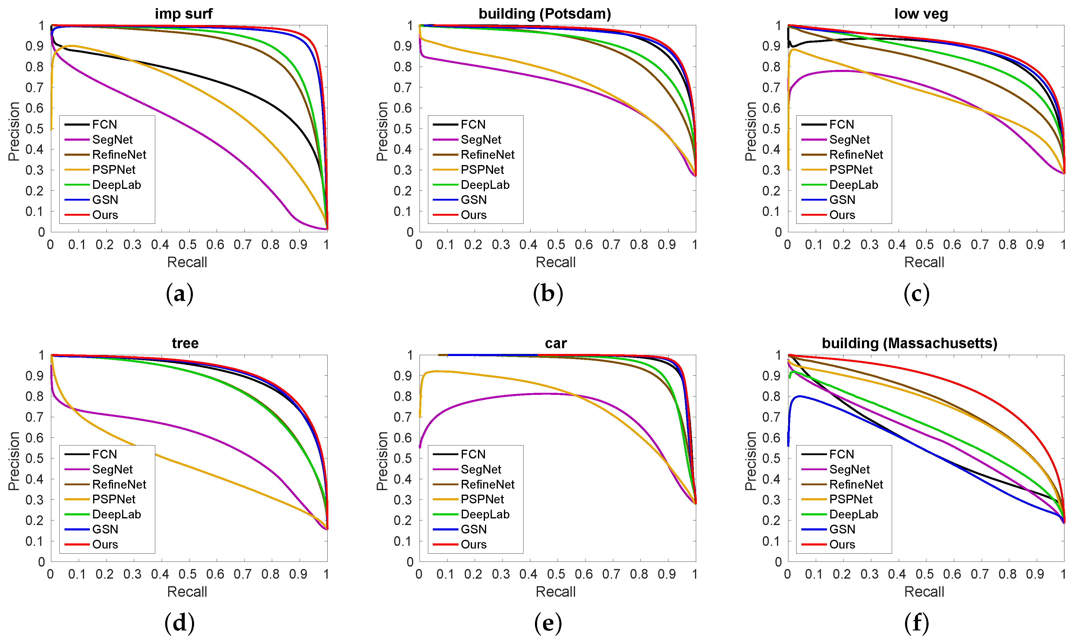
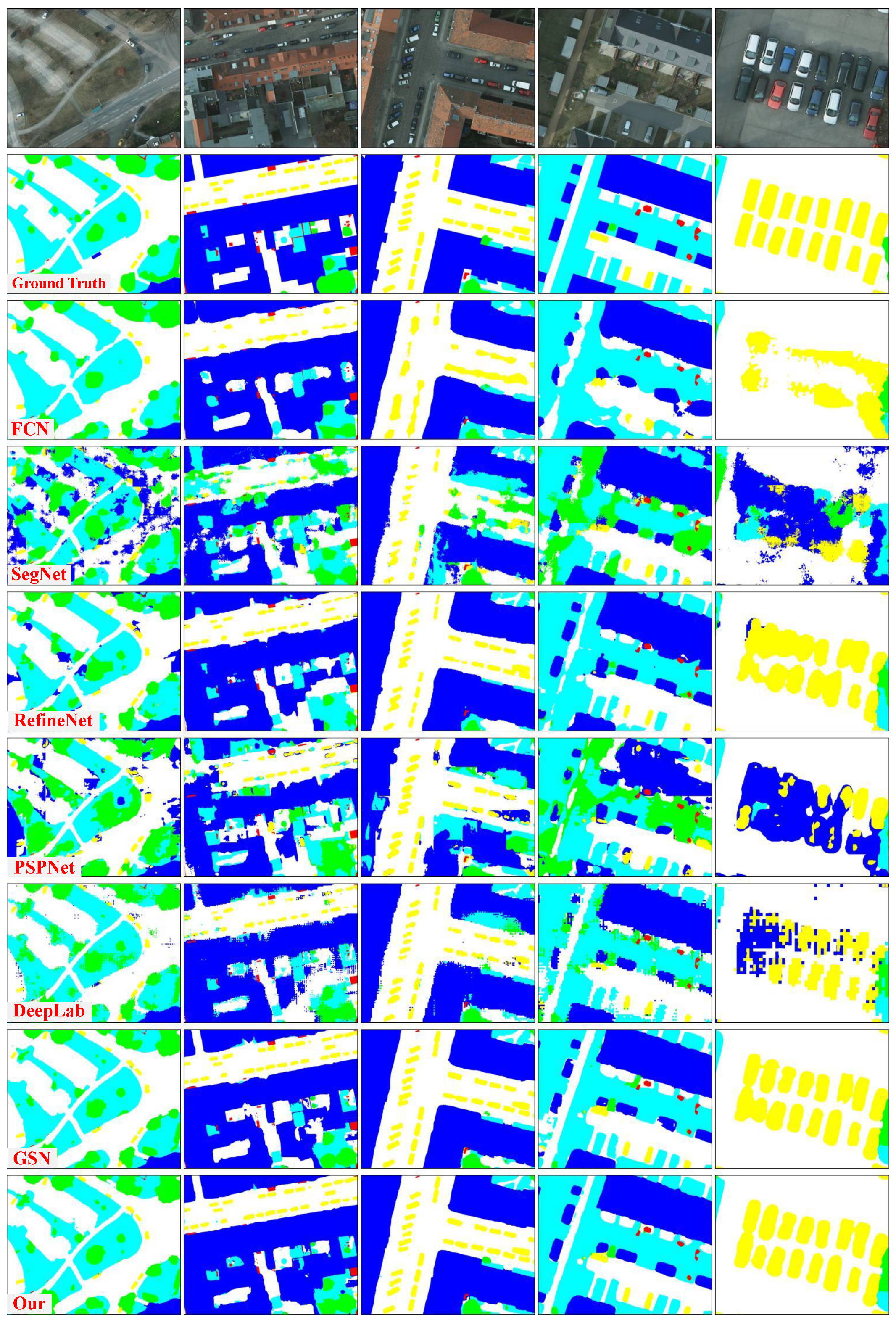
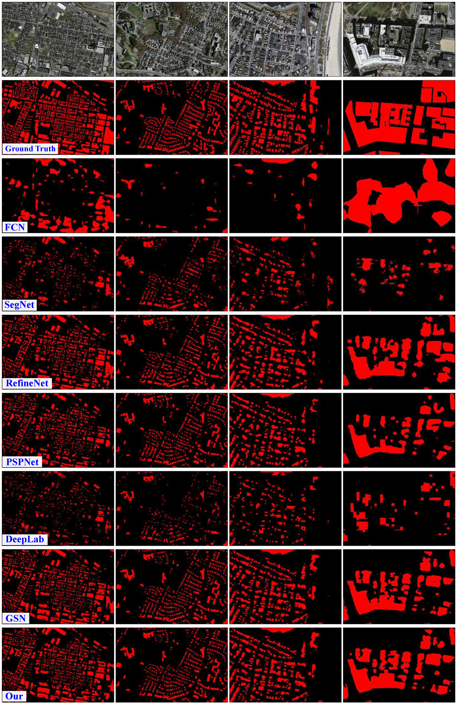
4.4. Experiment Results
5. Discussion
5.1. Result Analysis
- A gate function is proposed for multiscale feature fusion. The most distinct characteristic of our gate function lies in that it is a parameterized formulation of the Taylor expression of the information-entropy function. Beyond the entropy function with no parameters, our gate function has learnable parameters that can be learned from data. This helps increase the representation capability of our proposed L-GCNN.
- The design of a single PGM and its densely connected counterpart were embedded, respectively, into multilevels of the encoder in the L-GCNN. This strategy yields a multitask learning framework for gating multiscale information fusion, from which discriminative features can be extracted at multiscales of receptive fields.
- Topologically, our L-GCNN is a self-cascaded end-to-end architecture that is able to sequentially aggregate context information. Upon this architecture, pixelwise importance identified by the PGMs can be transferred from high to low level, achieving global-to-local refinement for the semantical segmentation of remote-sensing objects.
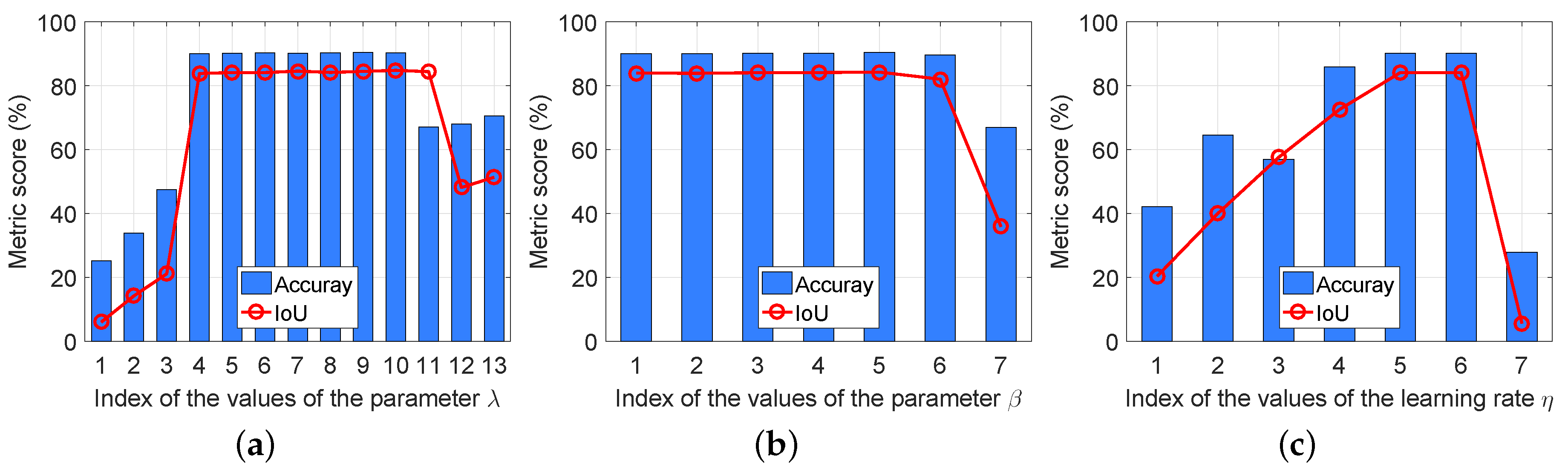
5.2. Parameter Sensitivity
5.3. Model Complexity
5.4. Implications and Limitations
- As reported in Table 7, the L-GCNN has more than 54 million network parameters. Such a huge model requires to be trained with high-performance computing resources (like a computing server with GPUs), which limits its usage in real-time semantical segmentation, embedded systems and other situations with limited computational resource like those on orbiting satellites. This drawback could be overcome by using the technique of model compression and more effective topology with neural architecture search.
- The L-GCNN should be trained with a large number of samples. For example, on the Potsdam dataset, there were 8000 samples in total, well-labeled for training. That is, good performance may not be guaranteed due to the small size of sample sets. However, in the field of RS image processing, public samples with truthful ground truth are very limited. One way to overcome this point is to embed prior knowledge related to the task of semantic segmentation into the network. Another way is to employ a generative adversarial network to yield more samples.
- The L-GCNN has no capability to treat new situations with different sample distributions and unseen categories. Its performance could largely be reduced on unseen or adversarial samples. In the future, its generalization power could be overcome by introducing a mechanism in the network to allow online learning in terms of domain adaption, deep transfer learning and deep reinforcement learning.
6. Conclusions
Author Contributions
Funding
Conflicts of Interest
References
- Bruzzone, L.; Demir, B. A review of modern approaches to classification of remote sensing data. In Land Use and Land Cover Mapping in Europe; Springer: Berlin/Heidelberg, Germany, 2014; pp. 127–143. [Google Scholar]
- Ghamisi, P.; Dalla Mura, M.; Benediktsson, J.A. A survey on spectral–spatial classification techniques based on attribute profiles. IEEE Trans. Geosci. Remote Sens. 2015, 53, 2335–2353. [Google Scholar] [CrossRef]
- Zhang, L.; Zhang, L.; Du, B. Deep learning for remote sensing data: A technical tutorial on the state of the art. IEEE Geosci. Remote Sens. Mag. 2016, 4, 22–40. [Google Scholar] [CrossRef]
- Cheng, G.; Han, J.; Lu, X. Remote Sensing Image Scene Classification: Benchmark and State of the Art. arXiv 2017, arXiv:1703.00121. [Google Scholar] [CrossRef]
- Sladojevic, S.; Arsenovic, M.; Anderla, A.; Culibrk, D.; Stefanovic, D. Deep Neural Networks Based Recognition of Plant Diseases by Leaf Image Classification. Comput. Intell. Neurosci. 2016, 2016, 3289801. [Google Scholar] [CrossRef] [PubMed]
- Singh, V.; Misra, A. Detection of plant leaf diseases using image segmentation and soft computing techniques. Inf. Process. Agric. 2017, 4, 41–49. [Google Scholar] [CrossRef] [Green Version]
- Lu, J.; Hu, J.; Zhao, G.; Mei, F.; Zhang, C. An in-field automatic wheat disease diagnosis system. Comput. Electron. Agric. 2017, 142, 369–379. [Google Scholar] [CrossRef] [Green Version]
- Golhani, K.; Balasundram, S.K.; Vadamalai, G.; Pradhan, B. A review of neural networks in plant disease detection using hyperspectral data. Inf. Proc. Agric. 2018, 5, 354–371. [Google Scholar] [CrossRef]
- Al-Saddik, H.; Laybros, A.; Billiot, B.; Cointault, F. Using Image Texture and Spectral Reflectance Analysis to Detect Yellowness and Esca in Grapevines at Leaf-Level. Remote Sens. 2018, 10, 618. [Google Scholar] [CrossRef]
- Dang, L.M.; Hassan, S.I.; Suhyeon, I.; Sangaiah, A.K.; Mehmood, I.; Rho, S.; Seo, S.; Moon, H. UAV based wilt detection system via convolutional neural networks. Sustain. Comput. Inf. Syst. 2019. [Google Scholar] [CrossRef]
- Matikainen, L.; Karila, K. Segment-based land cover mapping of a suburban area-comparison of high-resolution remotely sensed datasets using classification trees and test field points. Remote Sens. 2011, 3, 1777–1804. [Google Scholar] [CrossRef]
- Wen, D.; Huang, X.; Liu, H.; Liao, W.; Zhang, L. Semantic Classification of Urban Trees Using Very High Resolution Satellite Imagery. IEEE J. Sel. Top. Appl. Earth Obs. Remote Sens. 2017, 10, 1413–1424. [Google Scholar] [CrossRef]
- Xie, F.; Shi, M.; Shi, Z.; Yin, J.; Zhao, D. Multilevel Cloud Detection in Remote Sensing Images Based on Deep Learning. IEEE J. Sel. Top. Appl. Earth Obs. Remote Sens. 2017, 10, 3631–3640. [Google Scholar] [CrossRef]
- Liu, C.C.; Zhang, Y.C.; Chen, P.Y.; Lai, C.C.; Chen, Y.H.; Cheng, J.H.; Ko, M.H. Clouds Classification from Sentinel-2 Imagery with Deep Residual Learning and Semantic Image Segmentation. Remote Sens. 2019, 11, 119. [Google Scholar] [CrossRef]
- Zhang, P.; Gong, M.; Su, L.; Liu, J.; Li, Z. Change detection based on deep feature representation and mapping transformation for multi-spatial-resolution remote sensing images. ISPRS J. Photogramm. Remote Sens. 2016, 116, 24–41. [Google Scholar] [CrossRef]
- Lu, X.; Yuan, Y.; Zheng, X. Joint Dictionary Learning for Multispectral Change Detection. IEEE Trans. Cybern. 2017, 47, 884–897. [Google Scholar] [CrossRef]
- Tang, Y.; Zhang, L. Urban change analysis with multi-sensor multispectral imagery. Remote Sens. 2017, 9, 252. [Google Scholar] [CrossRef]
- Audebert, N.; Saux, B.L.; Lefevre, S. Segment-before-Detect: Vehicle Detection and Classification through Semantic Segmentation of Aerial Images. Remote Sens. 2017, 9, 368. [Google Scholar] [CrossRef]
- Li, E.; Femiani, J.; Xu, S.; Zhang, X.; Wonka, P. Robust Rooftop Extraction From Visible Band Images Using Higher Order CRF. IEEE Trans. Geosci. Remote Sens. 2015, 53, 4483–4495. [Google Scholar] [CrossRef]
- Xu, S.; Pan, X.; Li, E.; Wu, B.; Bu, S.; Dong, W.; Xiang, S.; Zhang, X. Automatic Building Rooftop Extraction From Aerial Images via Hierarchical RGB-D Priors. IEEE Trans. Geosci. Remote Sens. 2018, 56, 7369–7387. [Google Scholar] [CrossRef]
- Zhang, Z.; Liu, Q.; Wang, Y. Road Extraction by Deep Residual U-Net. IEEE Geosci. Remote Sens. Lett. 2018, 15, 749–753. [Google Scholar] [CrossRef]
- Xu, Y.; Xie, Z.; Feng, Y.; Chen, Z. Road Extraction from High-Resolution Remote Sensing Imagery Using Deep Learning. Remote Sens. 2018, 10, 1416. [Google Scholar] [CrossRef]
- LeCun, Y.; Bottou, L.; Bengio, Y.; Haffner, P. Gradient-Based Learning Applied to Document Recognition. Proc. IEEE 1998, 86, 2278–2324. [Google Scholar] [CrossRef]
- Long, J.; Shelhamer, E.; Darrell, T. Fully convolutional networks for semantic segmentation. IEEE Trans. Pattern Anal. Mach. Intell. 2015, 79, 1337–1342. [Google Scholar]
- Ronneberger, O.; Fischer, P.; Brox, T. U-net: Convolutional networks for biomedical image segmentation. In Proceedings of the International Conference on Medical Image Computing and Computer-Assisted Intervention, Munich, Germany, 5–9 October 2015; Springer: Berlin/Heidelberg, Germany, 2015; pp. 234–241. [Google Scholar]
- Badrinarayanan, V.; Kendall, A.; Cipolla, R. Segnet: A deep convolutional encoder-decoder architecture for image segmentation. arXiv 2015, arXiv:1511.00561. [Google Scholar] [CrossRef] [PubMed]
- Noh, H.; Hong, S.; Han, B. Learning Deconvolution Network for Semantic Segmentation. In Proceedings of the IEEE International Conference on Computer Vision, Las Condes, Chile, 11–18 December 2015; pp. 1520–1528. [Google Scholar]
- Lin, G.; Milan, A.; Shen, C.; Reid, I.D. RefineNet: Multi-Path Refinement Networks for High-Resolution Semantic Segmentation. arXiv 2016, arXiv:1611.06612. [Google Scholar]
- Chen, L.C.; Papandreou, G.; Kokkinos, I.; Murphy, K.; Yuille, A.L. Deeplab: Semantic image segmentation with deep convolutional nets, atrous convolution, and fully connected crfs. IEEE Trans. Pattern Anal. Mach. Intell. 2018, 40, 834–848. [Google Scholar] [CrossRef] [PubMed]
- Wang, H.; Wang, Y.; Zhang, Q.; Xiang, S.; Pan, C. Gated Convolutional Neural Network for Semantic Segmentation in High-Resolution Images. Remote Sens. 2017, 9, 446. [Google Scholar] [CrossRef] [Green Version]
- Liu, Y.; Fan, B.; Wanga, L.; Bai, J.; Xiang, S.; Pan, C. Semantic Labeling in very High Resolution Images via A Self-cascaded Convolutional Neural Network. ISPRS J. Photogramm. Remote Sens. 2018, 145, 78–95. [Google Scholar] [CrossRef]
- Li, L.; Yao, J.; Liu, Y.; Yuan, W.; Shi, S.; Yuan, S. Optimal Seamline Detection for Orthoimage Mosaicking by Combining Deep Convolutional Neural Network and Graph Cuts. Remote Sens. 2017, 9, 701. [Google Scholar] [CrossRef]
- Panboonyuen, T.; Jitkajornwanich, K.; Lawawirojwong, S.; Srestasathiern, P.; Vateekul, P. Semantic Segmentation on Remotely Sensed Images Using an Enhanced Global Convolutional Network with Channel Attention and Domain Specific Transfer Learning. Remote Sens. 2019, 11, 83. [Google Scholar] [CrossRef]
- Goodfellow, I.; Bengio, Y.; Courville, A. Deep Learning; MIT Press: Cambridge, MA, USA, 2016. [Google Scholar]
- Zhao, H.; Shi, J.; Qi, X.; Wang, X.; Jia, J. Pyramid Scene Parsing Network. arXiv 2016, arXiv:1612.01105. [Google Scholar]
- Sherrah, J. Fully convolutional networks for dense semantic labelling of highresolution aerial imagery. arXiv 2016, arXiv:1606.02585. [Google Scholar]
- Alshehhi, R.; Marpu, P.R.; Woon, W.L.; Mura, M.D. Simultaneous extraction of roads and buildings in remote sensing imagery with convolutional neural networks. ISPRS J. Photogramm. Remote Sens. 2017, 130, 139–149. [Google Scholar] [CrossRef]
- Chen, K.; Fu, K.; Yan, M.; Gao, X.; Sun, X.; Wei, X. Semantic Segmentation of Aerial Images With Shuffling Convolutional Neural Networks. IEEE Geosci. Remote Sens. Lett. 2018, 15, 173–177. [Google Scholar] [CrossRef]
- Chen, G.; Zhang, X.; Wang, Q.; Dai, F.; Gong, Y.; Zhu, K. Symmetrical Dense-Shortcut Deep Fully Convolutional Networks for Semantic Segmentation of Very-High-Resolution Remote Sensing Images. IEEE J. Sel. Top. Appl. Earth Obs. Remote Sens. 2018, 11, 1633–1644. [Google Scholar] [CrossRef]
- Persello, C.; Stein, A. Deep Fully Convolutional Networks for the Detection of Informal Settlements in VHR Images. IEEE Geosci. Remote Sens. Lett. 2017, 14, 2325–2329. [Google Scholar] [CrossRef] [Green Version]
- Yuan, J. Learning Building Extraction in Aerial Scenes with Convolutional Networks. IEEE Trans. Pattern Anal. Mach. Intell. 2018, 40, 2793–2798. [Google Scholar] [CrossRef]
- He, K.; Zhang, X.; Ren, S.; Sun, J. Deep residual learning for image recognition. In Proceedings of the IEEE Conference on Computer Vision and Pattern Recognition, Las Vegas, NV, USA, 26 June–1 July 2016; pp. 770–778. [Google Scholar]
- Hu, J.; Shen, L.; Sun, G. Squeeze-and-Excitation Networks. In Proceedings of the IEEE International Conference on Computer Vision and Pattern Recognition, Salt Lake City, UT, USA, 18–22 June 2018; pp. 7132–7141. [Google Scholar]
- ISPRS. 2D Semantic Labeling Challenge by International Society for Photogrammetry and Remote Sensing. Available online: http://www2.isprs.org/commissions/comm3/wg4/semantic-labeling.html (accessed on 16 August 2019).
- Mnih, V. Machine Learning for Aerial Image Labeling. Ph.D. Thesis, University of Toronto, Toronto, ON, Canada, 2013. [Google Scholar]
- Yosinski, J.; Clune, J.; Bengio, Y.; Lipson, H. How Transferable are Features in Deep Neural Networks. In Neural Information Processing Systems; Mit Press: Cambridge, MA, USA, 2014; pp. 3320–3328. [Google Scholar]
- Penatti, O.A.; Nogueira, K.; dos Santos, J.A. Do deep features generalize from everyday objects to remote sensing and aerial scenes domains. In Proceedings of the IEEE Conference on Computer Vision and Pattern Recognition Workshop, Boston, MA, USA, 7–12 June 2015; pp. 44–51. [Google Scholar]
- Everingham, M.; Eslami, S.M.A.; Gool, L.J.V.; Williams, C.K.I.; Winn, J.M.; Zisserman, A. The Pascal Visual Object Classes Challenge: A Retrospective. Int. J. Comput. Vis. 2015, 111, 98–136. [Google Scholar] [CrossRef]


| Method | Level 1 | Level 2 | Level 3 | Level 4 | Level 5 |
|---|---|---|---|---|---|
| Resnet101 | |||||
| SCM1 | |||||
| SEM | |||||
| PGM | |||||
| SCM2 | |||||
| DC-PGM | |||||
| Conv |
| Model | Imp Surf | Building | Low Veg | Tree | Car | Average |
|---|---|---|---|---|---|---|
| FCN | 88.31 | 93.09 | 83.26 | 82.10 | 73.05 | 83.96 |
| SegNet | 85.29 | 88.62 | 81.78 | 78.49 | 64.55 | 79.75 |
| RefineNet | 88.80 | 92.84 | 84.41 | 82.62 | 87.04 | 87.14 |
| PSPNet | 74.24 | 75.29 | 64.41 | 47.14 | 41.79 | 60.57 |
| DeepLab | 89.92 | 93.44 | 84.84 | 83.74 | 90.97 | 88.58 |
| GSN | 91.69 | 95.05 | 86.63 | 85.23 | 91.68 | 90.05 |
| L-GCNN (our) | 92.84 | 96.17 | 87.78 | 85.74 | 93.65 | 91.24 |
| Model | Imp Surf | Building | Low Veg | Tree | Car | Average |
|---|---|---|---|---|---|---|
| FCN | 79.08 | 87.08 | 71.31 | 69.63 | 57.53 | 72.93 |
| SegNet | 74.36 | 79.57 | 69.17 | 64.60 | 47.66 | 67.07 |
| RefineNet | 79.86 | 86.65 | 73.03 | 70.38 | 77.05 | 77.39 |
| PSPNet | 59.04 | 60.37 | 47.50 | 30.83 | 26.41 | 44.83 |
| DeepLab | 81.69 | 87.69 | 73.67 | 72.02 | 83.42 | 79.70 |
| GSN | 84.43 | 90.45 | 76.42 | 72.28 | 84.30 | 81.58 |
| L-GCNN (our) | 86.64 | 92.62 | 78.21 | 75.04 | 88.06 | 84.12 |
| Metrics | FCN | SegNet | RefineNet | PSPNet | DeepLab | GSN | L-GCNN (Our) |
|---|---|---|---|---|---|---|---|
| F1 | 70.29 | 65.47 | 82.38 | 79.73 | 77.58 | 83.68 | 85.73 |
| IoU | 58.01 | 54.22 | 71.59 | 68.50 | 65.90 | 73.29 | 76.15 |
| Model | Imp Surf | Building | Low Veg | Tree | Car | |||||
|---|---|---|---|---|---|---|---|---|---|---|
| Accu | IoU | Accu | IoU | Accu | IoU | Accu | IoU | Accu | IoU | |
| 91.45 | 85.00 | 96.23 | 90.87 | 86.18 | 76.35 | 83.94 | 74.46 | 90.25 | 86.53 | |
| 91.50 | 85.21 | 96.39 | 91.19 | 86.03 | 76.05 | 86.48 | 74.93 | 90.16 | 86.35 | |
| 90.36 | 84.65 | 95.74 | 90.60 | 86.33 | 76.77 | 83.34 | 74.44 | 90.36 | 86.65 | |
| 91.42 | 85.07 | 96.84 | 91.19 | 86.20 | 76.49 | 84.98 | 74.78 | 93.01 | 86.76 | |
| 90.99 | 84.97 | 96.54 | 91.35 | 86.30 | 76.69 | 86.05 | 74.66 | 93.85 | 86.27 | |
| Model | Imp Surf | Building | Low Veg | Tree | Car | |||||
|---|---|---|---|---|---|---|---|---|---|---|
| Accu | IoU | Accu | IoU | Accu | IoU | Accu | IoU | Accu | IoU | |
| Reduced Model | 90.13 | 80.71 | 94.49 | 88.92 | 85.94 | 74.63 | 83.86 | 72.64 | 91.35 | 82.88 |
| L-GCNN | 91.42 | 85.07 | 96.84 | 91.19 | 86.20 | 76.49 | 84.98 | 74.78 | 93.01 | 86.76 |
| FCN | SegNet | RefineNet | PSPNet | DeepLab | GSN | L-GCNN (Our) | |
|---|---|---|---|---|---|---|---|
| #FLOPs (GMACs) | 124.80 | 90.74 | 140.18 | 157.22 | 100.89 | 44.16 | 46.16 |
| #parameters (M) | 134 | 29 | 71 | 72 | 42 | 53 | 54 |
| Averaged test time (ms) | 33.56 | 20.47 | 38.08 | 57.23 | 54.89 | 29.52 | 31.47 |
© 2019 by the authors. Licensee MDPI, Basel, Switzerland. This article is an open access article distributed under the terms and conditions of the Creative Commons Attribution (CC BY) license (http://creativecommons.org/licenses/by/4.0/).
Share and Cite
Guo, S.; Jin, Q.; Wang, H.; Wang, X.; Wang, Y.; Xiang, S. Learnable Gated Convolutional Neural Network for Semantic Segmentation in Remote-Sensing Images. Remote Sens. 2019, 11, 1922. https://0-doi-org.brum.beds.ac.uk/10.3390/rs11161922
Guo S, Jin Q, Wang H, Wang X, Wang Y, Xiang S. Learnable Gated Convolutional Neural Network for Semantic Segmentation in Remote-Sensing Images. Remote Sensing. 2019; 11(16):1922. https://0-doi-org.brum.beds.ac.uk/10.3390/rs11161922
Chicago/Turabian StyleGuo, Shichen, Qizhao Jin, Hongzhen Wang, Xuezhi Wang, Yangang Wang, and Shiming Xiang. 2019. "Learnable Gated Convolutional Neural Network for Semantic Segmentation in Remote-Sensing Images" Remote Sensing 11, no. 16: 1922. https://0-doi-org.brum.beds.ac.uk/10.3390/rs11161922