Multi-Hazard Exposure Mapping Using Machine Learning Techniques: A Case Study from Iran

 ,
,  , , ,
, , ,  , and
, and
Abstract
:
1. Introduction
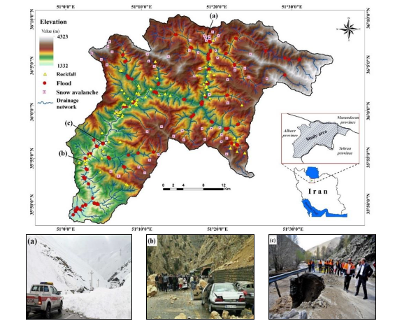
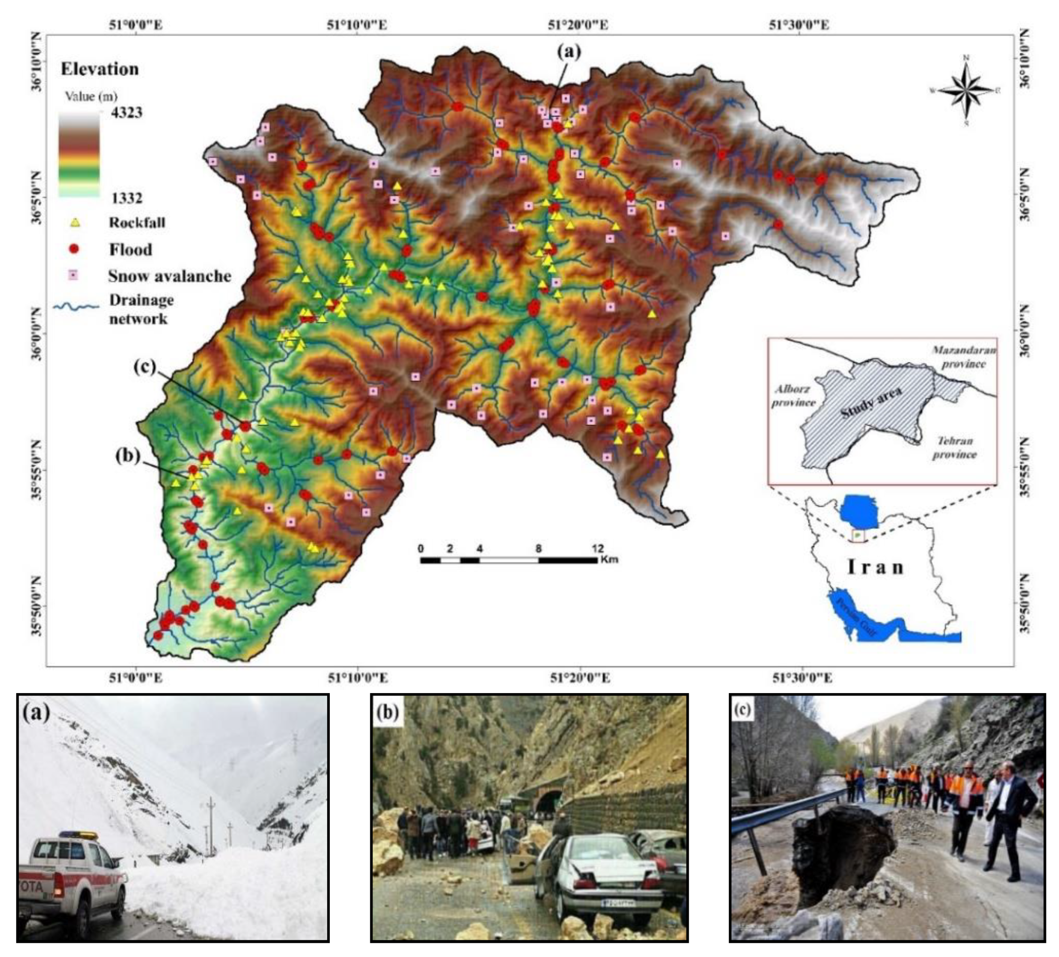
2. Study Area
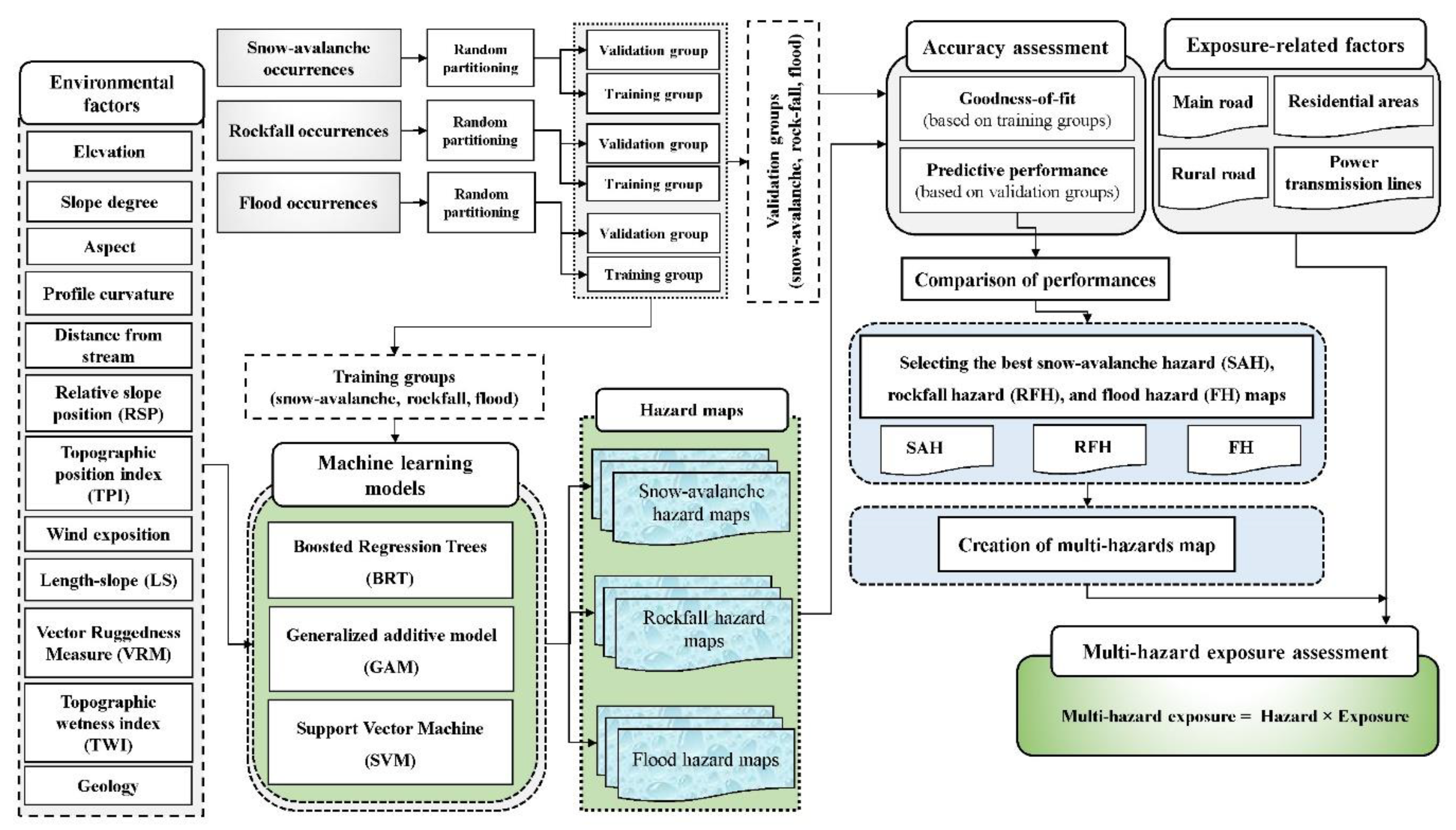
3. Methodology
3.1. Multi-Hazard Modelling
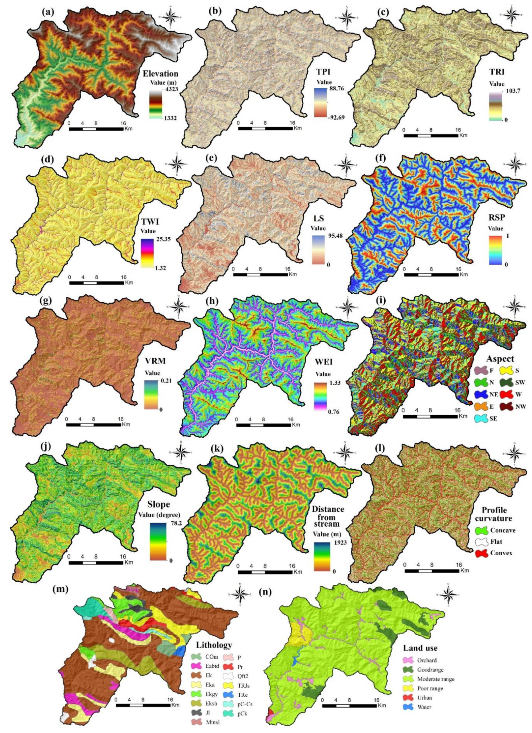
3.1.1. Predictive Factors
3.1.2. Multi-Hazard Inventory
3.1.3. Application of Models
Generalized Additive Model (GAM)
Boosted Regression Tree (BRT)
Support Vector Machine (SVM)
3.1.4. Accuracy Assessment
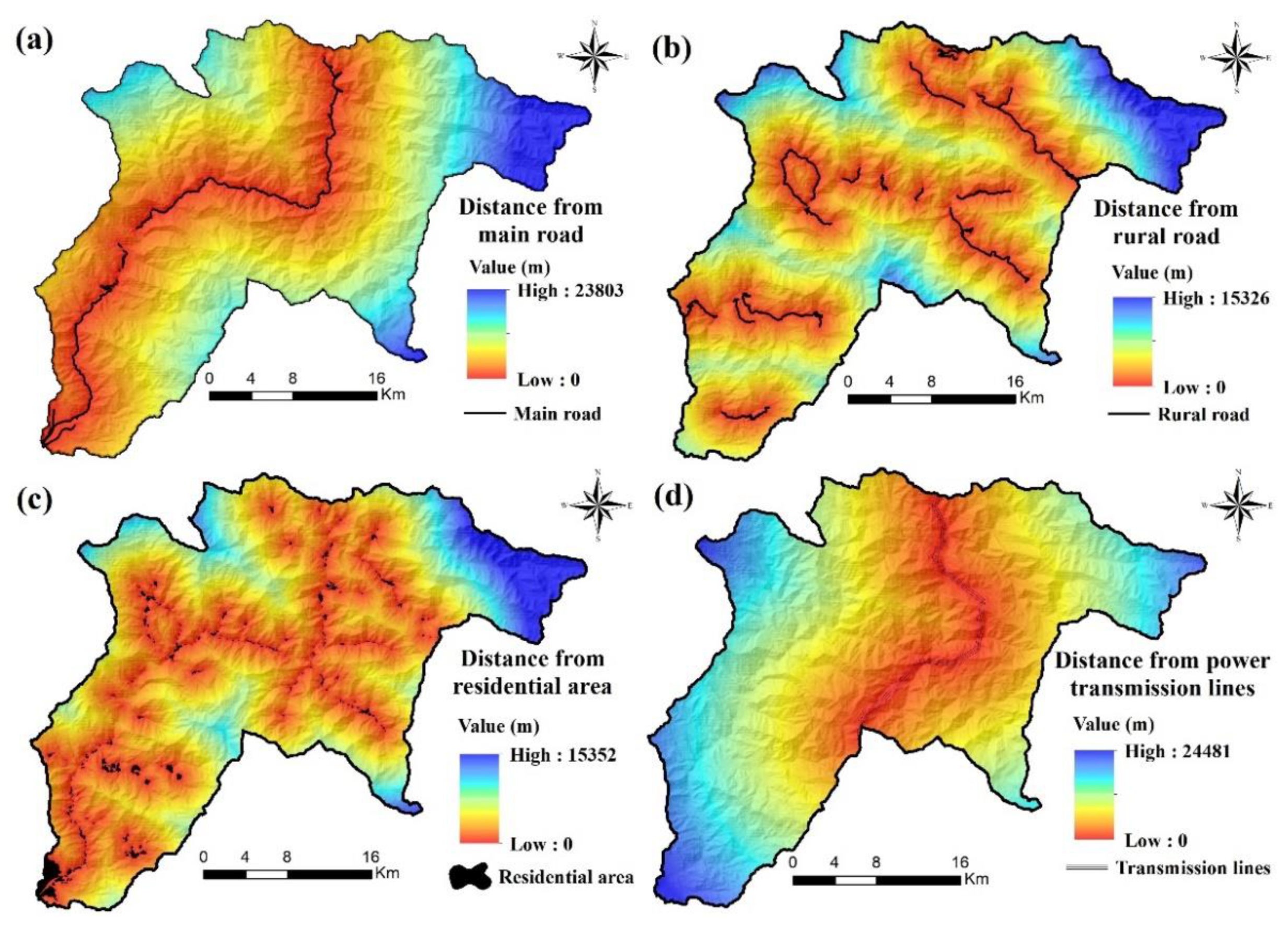
3.2. Exposure-Related Factors
3.3. Multi-Hazard Exposure Mapping
4. Results
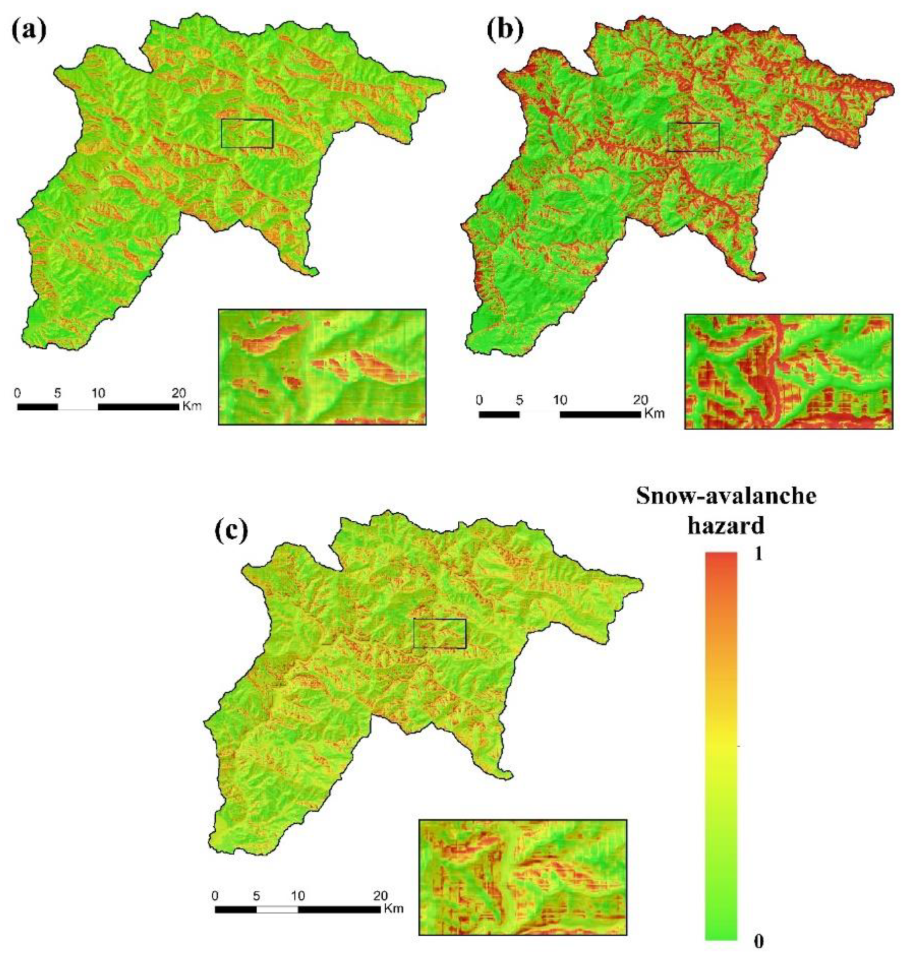
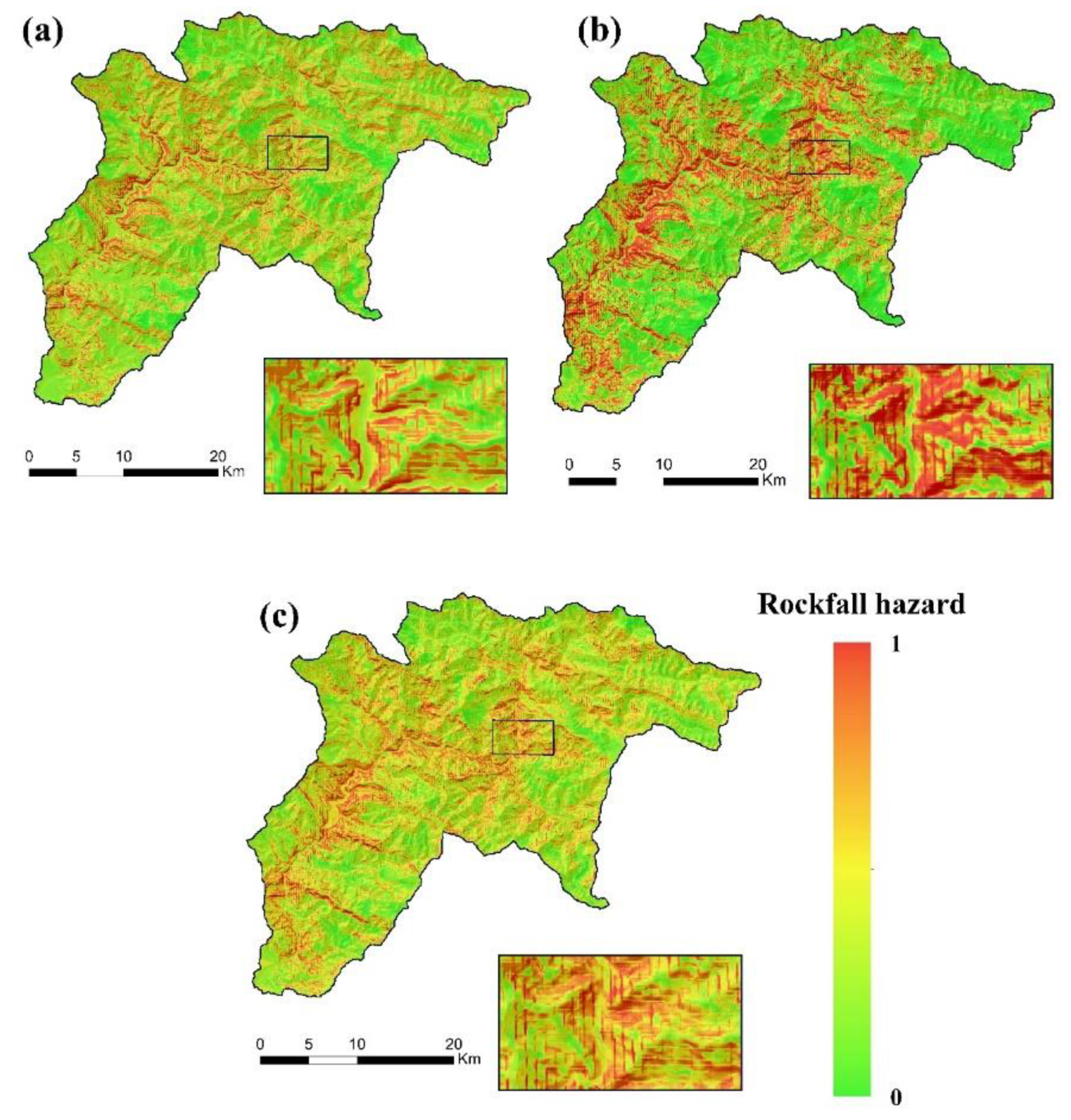
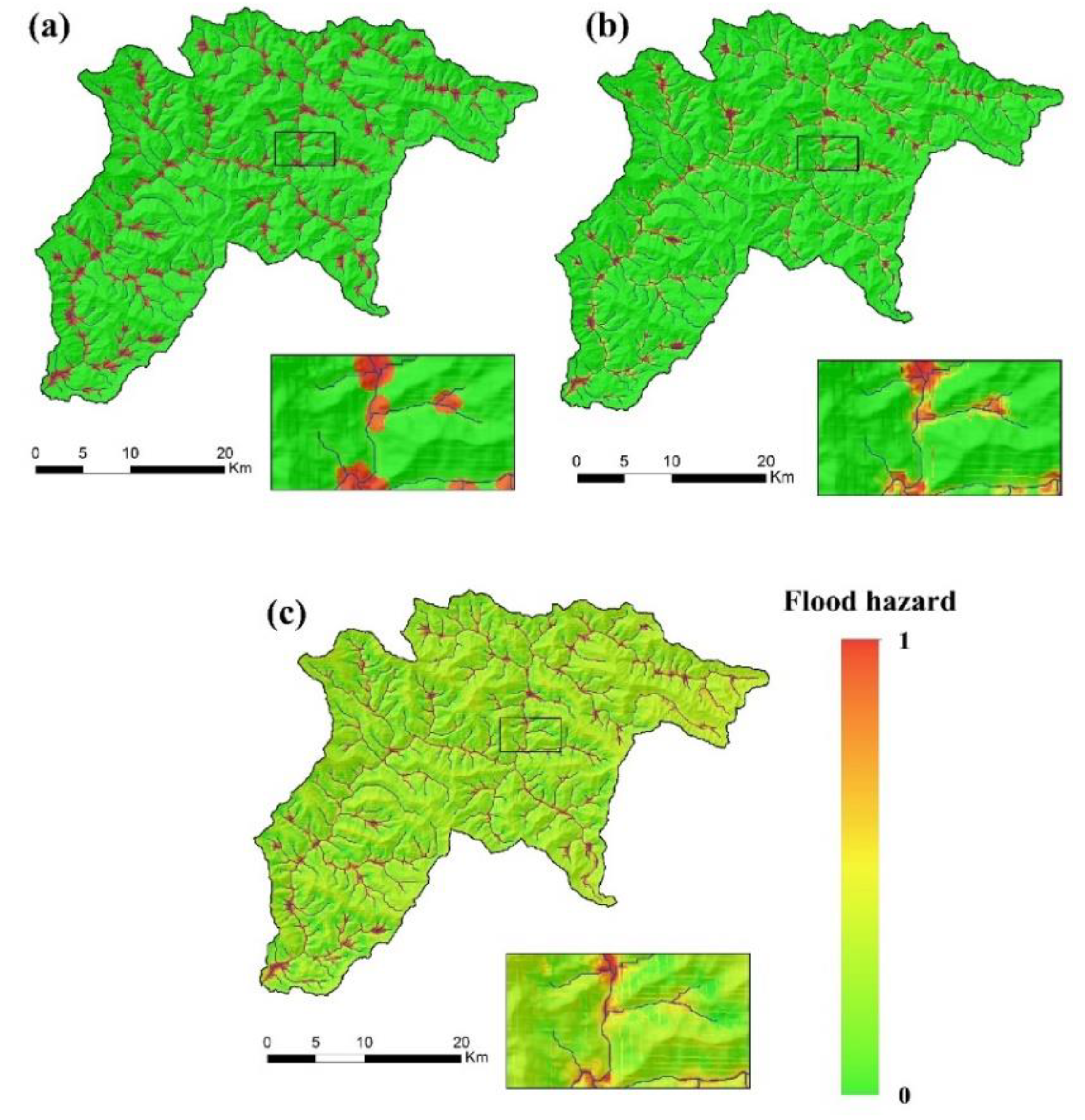
4.1. Hazard Maps
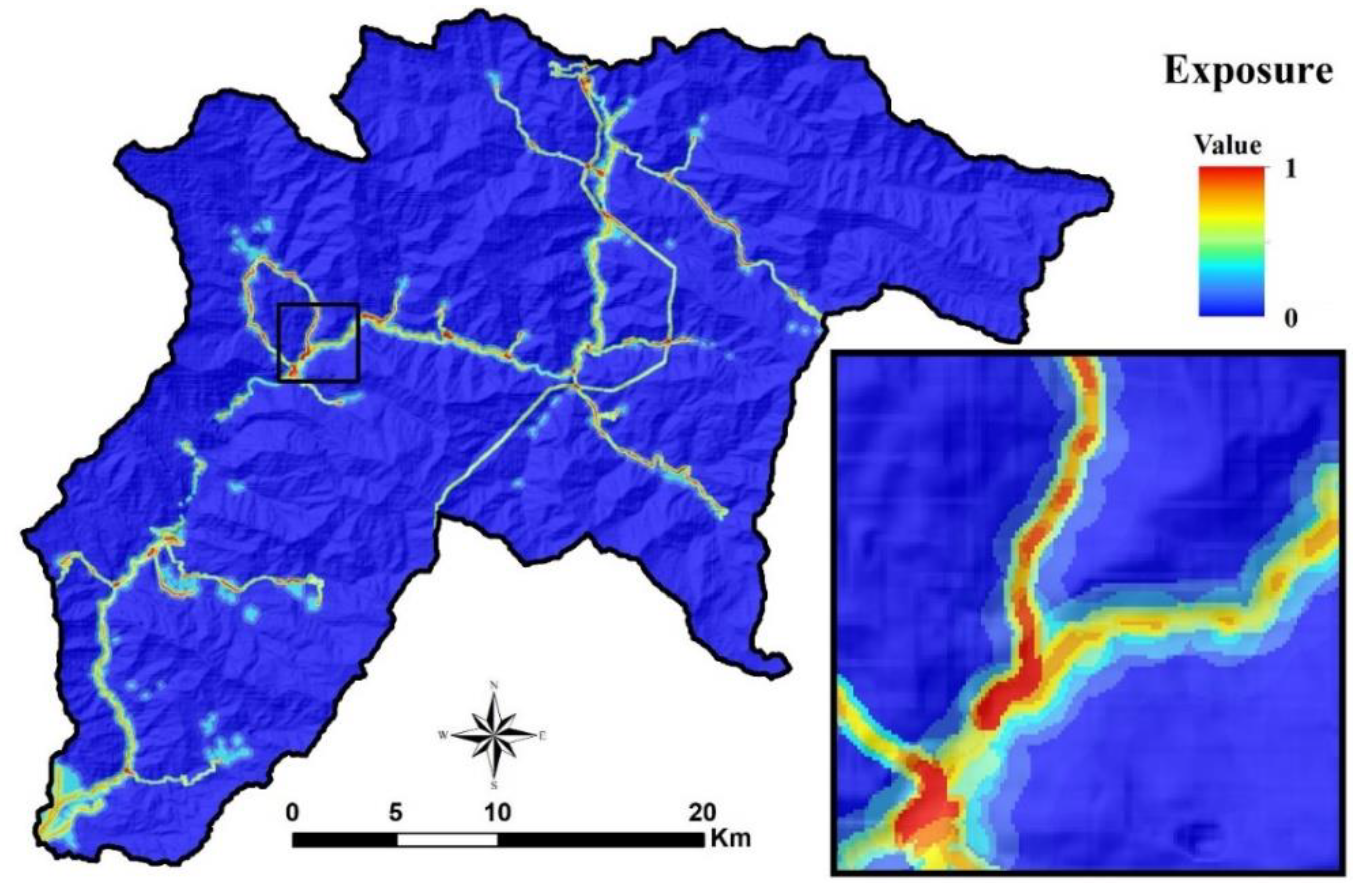
4.2. Exposure Map
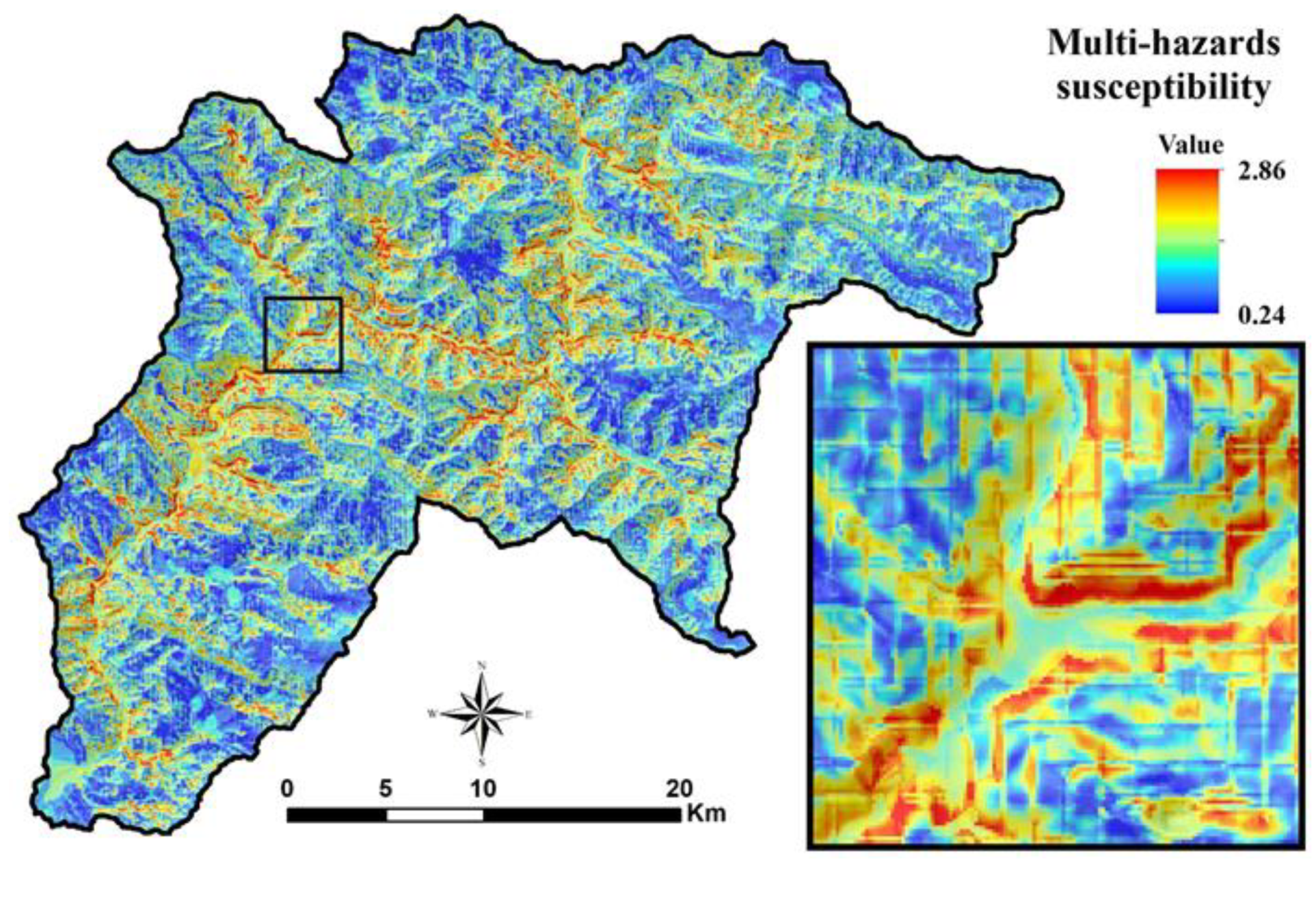
4.3. Multi-Hazard Exposure Map
5. Discussion
6. Conclusions
Author Contributions
Funding
Acknowledgments
Conflicts of Interest
References
- Fuchs, S.; Keiler, M.; Zischg, A. A spatiotemporal multi-hazard exposure assessment based on property data. Nat. Hazards Earth Syst. Sci. 2015, 15, 2127–2142. [Google Scholar] [CrossRef] [Green Version]
- Barthel, F.; Neumayer, E. A trend analysis of normalized insured damage from natural disasters. Clim. Chang. 2012, 113, 215–237. [Google Scholar] [CrossRef]
- Munich, R.E.; Kron, W.; Schuck, A. Topics Geo: Natural Catastrophes 2013: Analyses, Assessments, Positions; Munchener Ruckversicherungs-Gesellschaft: Munich, Germany, 2014. [Google Scholar]
- Bell, R.; Glade, T. Multi-hazard analysis in natural risk assessments. In Landslides; Safety & Security Engineering Series; WIT Press: Southampton, UK, 2012; pp. 1–10. [Google Scholar]
- Michielsen, A.; Kalantari, Z.; Lyon, S.W.; Liljegren, E. Predicting and communicating flood risk of transport infrastructure based on watershed characteristics. J. Environ. Manag. 2016, 182, 505–518. [Google Scholar] [CrossRef] [PubMed]
- McGuire, K.J.; McDonnell, J.J. Hydrological connectivity of hillslopes and streams: Characteristic time scales and nonlinearities. Water Resour. Res. 2010, 46. [Google Scholar] [CrossRef] [Green Version]
- Nikolopoulos, E.I.; Anagnostou, E.N.; Borga, M.; Vivoni, E.R.; Papadopoulos, A. Sensitivity of a mountain basin flash flood to initial wetness condition and rainfall variability. J. Hydrol. 2011, 402, 165–178. [Google Scholar] [CrossRef]
- Jamieson, B.; Stethem, C. Snow avalanche hazards and management in Canada: challenges and progress. Nat. Hazards 2002, 26, 35–53. [Google Scholar] [CrossRef]
- Corona, C.; Stoffel, M. Snow and Ice Avalanches. In International Encyclopedia of Geography: People, the Earth, Environment and Technology; John Wiley & Sons, Ltd.: Hoboken, NJ, USA, 2017; pp. 1–7. [Google Scholar]
- Meseșan, F.; Man, T.C.; Pop, O.T.; Gavrilă, I.G. Reconstructing snow-avalanche extent using remote sensing and dendrogeomorphology in Parâng Mountains. Cold Reg. Sci. Technol. 2019, 157, 97–109. [Google Scholar] [CrossRef]
- Pourghasemi, H.R.; Pradhan, B.; Gokceoglu, C. Application of fuzzy logic and analytical hierarchy process (AHP) to landslide susceptibility mapping at Haraz watershed, Iran. Nat. Hazards 2012, 63, 965–996. [Google Scholar] [CrossRef]
- Dehnavi, A.; Aghdam, I.N.; Pradhan, B.; Morshed Varzandeh, M.H. A new hybrid model using step-wise weight assessment ratio analysis (SWARA) technique and adaptive neuro-fuzzy inference system (ANFIS) for regional landslide hazard assessment in Iran. Catena 2015, 135, 122–148. [Google Scholar] [CrossRef]
- Suresh, D.; Yarrakula, K.; Venkateswarlu, B.; Mohanty, B.; Manupati, V. Risk Mapping Analysis With Geographic Information Systems for Landslides Using Supply Chain. In Emerging Applications in Supply Chains for Sustainable Business Development; IGI Global: Hershey, PA, USA, 2019; pp. 131–141. [Google Scholar]
- Tien Bui, D.; Anh Tuan, T.; Hoang, N.-D.; Quoc Thanh, N.; Nguyen, B.D.; Van Liem, N.; Pradhan, B. Spatial Prediction of Rainfall-induced Landslides for the Lao Cai area (Vietnam) Using a Novel hybrid Intelligent Approach of Least Squares Support Vector Machines Inference Model and Artificial Bee Colony Optimization. Landslides 2017, 14, 447–458. [Google Scholar] [CrossRef]
- Barredo, J.I. Major flood disasters in Europe: 1950–2005. Nat. Hazards 2006, 42, 125–148. [Google Scholar] [CrossRef]
- Rahmati, O.; Zeinivand, H.; Besharat, M. Flood hazard zoning in Yasooj region, Iran, using GIS and multi-criteria decision analysis. Geomat. Nat. Hazards Risk 2015, 7, 1000–1017. [Google Scholar] [CrossRef] [Green Version]
- Shafizadeh-Moghadam, H.; Valavi, R.; Shahabi, H.; Chapi, K.; Shirzadi, A. Novel forecasting approaches using combination of machine learning and statistical models for flood susceptibility mapping. J. Environ. Manag. 2018, 217, 1–11. [Google Scholar] [CrossRef] [PubMed] [Green Version]
- Tien Bui, D.; Hoang, N.-D. A Bayesian framework based on a Gaussian mixture model and radial-basis-function Fisher discriminant analysis (BayGmmKda V1. 1) for spatial prediction of floods. Geosci. Model Dev. 2017, 10, 3391. [Google Scholar] [CrossRef]
- Glade, T. Linking debris-flow hazard assessments with geomorphology. Geomorphology 2005, 66, 189–213. [Google Scholar] [CrossRef]
- Sepúlveda, S.A.; Padilla, C. Rain-induced debris and mudflow triggering factors assessment in the Santiago cordilleran foothills, Central Chile. Nat. Hazards 2008, 47, 201–215. [Google Scholar] [CrossRef]
- Tsereteli, E.; Gaprindashvili, G.; Gaprindashvili, M.; Bolashvili, N.; Gongadze, M. Hazard Risk of Debris/Mud Flow Events in Georgia and Methodological Approaches for Management. In IAEG/AEG Annual Meeting Proceedings, San Francisco, California; Springer International Publishing: Basel, Switzerland, 2018; Volume 5, pp. 153–160. [Google Scholar]
- Pardini, G.; Gispert, M.; Dunjo, G. Runoff erosion and nutrient depletion in five Mediterranean soils of NE Spain under different land use. Sci. Total Environ. 2003, 309, 213–224. [Google Scholar] [CrossRef]
- Prasannakumar, V.; Vijith, H.; Abinod, S.; Geetha, N. Estimation of soil erosion risk within a small mountainous sub-watershed in Kerala, India, using Revised Universal Soil Loss Equation (RUSLE) and geo-information technology. Geosci. Front. 2012, 3, 209–215. [Google Scholar] [CrossRef] [Green Version]
- Prosdocimi, M.; Cerdà, A.; Tarolli, P. Soil water erosion on Mediterranean vineyards: A review. Catena 2016, 141, 1–21. [Google Scholar] [CrossRef]
- Michoud, C.; Derron, M.H.; Horton, P.; Jaboyedoff, M.; Baillifard, F.J.; Loye, A.; Nicolet, P.; Pedrazzini, A.; Queyrel, A. Rockfall hazard and risk assessments along roads at a regional scale: Example in Swiss Alps. Nat. Hazards Earth Syst. Sci. 2012, 12, 615–629. [Google Scholar] [CrossRef]
- Shirzadi, A.; Saro, L.; Hyun Joo, O.; Chapi, K. A GIS-based logistic regression model in rock-fall susceptibility mapping along a mountainous road: Salavat Abad case study, Kurdistan, Iran. Nat. Hazards 2012, 64, 1639–1656. [Google Scholar] [CrossRef] [Green Version]
- Losasso, L.; Jaboyedoff, M.; Sdao, F. Potential rock fall source areas identification and rock fall propagation in the province of Potenza territory using an empirically distributed approach. Landslides 2017, 14, 1593–1602. [Google Scholar] [CrossRef]
- Statham, G.; Haegeli, P.; Greene, E.; Birkeland, K.; Israelson, C.; Tremper, B.; Stethem, C.; McMahon, B.; White, B.; Kelly, J. A conceptual model of avalanche hazard. Nat. Hazards 2017, 90, 663–691. [Google Scholar] [CrossRef] [Green Version]
- Bühler, Y.; Christen, M.; Kowalski, J.; Bartelt, P. Sensitivity of snow avalanche simulations to digital elevation model quality and resolution. Ann. Glaciol. 2011, 52, 72–80. [Google Scholar] [CrossRef] [Green Version]
- Pourghasemi, H.R.; Yousefi, S.; Kornejady, A.; Cerdà, A. Performance assessment of individual and ensemble data-mining techniques for gully erosion modeling. Sci. Total Environ. 2017, 609, 764–775. [Google Scholar] [CrossRef] [Green Version]
- Rijsdijk, A.; Sampurno Bruijnzeel, L.A.; Sutoto, C.K. Runoff and sediment yield from rural roads, trails and settlements in the upper Konto catchment, East Java, Indonesia. Geomorphology 2007, 87, 28–37. [Google Scholar] [CrossRef]
- Spitz, W.; Lagasse, P.; Schumm, S.; Zevenbergen, L. A Methodology for Predicting Channel Migration NCHRP Project No. 24–16. In Wetlands Engineering & River Restoration 2001; American Society of Civil Engineers: Reston, VA, USA, 2001. [Google Scholar]
- Kalantari, Z.; Ferreira, C.S.S.; Koutsouris, A.J.; Ahmer, A.-K.; Cerdà, A.; Destouni, G. Assessing flood probability for transportation infrastructure based on catchment characteristics, sediment connectivity and remotely sensed soil moisture. Sci. Total Environ. 2019, 661, 393–406. [Google Scholar] [CrossRef]
- Gardner, J.S.; Dekens, J. Mountain hazards and the resilience of social–ecological systems: lessons learned in India and Canada. Nat. Hazards 2006, 41, 317–336. [Google Scholar] [CrossRef]
- Kalantari, Z.; Cavalli, M.; Cantone, C.; Crema, S.; Destouni, G. Flood probability quantification for road infrastructure: Data-driven spatial-statistical approach and case study applications. Sci. Total Environ. 2017, 581–582, 386–398. [Google Scholar] [CrossRef]
- Gruber, F.E.; Mergili, M. Regional-scale analysis of high-mountain multi-hazard and risk indicators in the Pamir (Tajikistan) with GRASS GIS. Nat. Hazards Earth Syst. Sci. 2013, 13, 2779–2796. [Google Scholar] [CrossRef] [Green Version]
- Karlsson, C.S.J.; Kalantari, Z.; Mörtberg, U.; Olofsson, B.; Lyon, S.W. Natural Hazard Susceptibility Assessment for Road Planning Using Spatial Multi-Criteria Analysis. Environ. Manag. 2017, 60, 823–851. [Google Scholar] [CrossRef] [Green Version]
- McClung, D.; Schaerer, P.A. The Avalanche Handbook; The Mountaineers Books: Seattle, WA, USA, 2006. [Google Scholar]
- Barbolini, M.; Pagliardi, M.; Ferro, F.; Corradeghini, P. Avalanche hazard mapping over large undocumented areas. Nat. Hazards 2009, 56, 451–464. [Google Scholar] [CrossRef]
- Van Westen, C.J.; Greiving, S. Multi-hazard risk assessment and decision making. In Environmental Hazards Methodologies for Risk Assessment and Management; IWA publishing: London, UK, 2017; pp. 31–94. [Google Scholar]
- Zhou, H.; Wan, J.; Jia, H. Resilience to natural hazards: a geographic perspective. Nat. Hazards 2010, 53, 21–41. [Google Scholar] [CrossRef]
- Demirkesen, A.C. Multi-risk interpretation of natural hazards for settlements of the Hatay province in the east Mediterranean region, Turkey using SRTM DEM. Environ. Earth Sci. 2012, 65, 1895–1907. [Google Scholar] [CrossRef]
- Zhou, Y.; Liu, Y.; Wu, W.; Li, N. Integrated risk assessment of multi-hazards in China. Nat. Hazards 2015, 78, 257–280. [Google Scholar] [CrossRef]
- Gallina, V.; Torresan, S.; Critto, A.; Sperotto, A.; Glade, T.; Marcomini, A. A review of multi-risk methodologies for natural hazards: Consequences and challenges for a climate change impact assessment. J. Environ. Manag. 2016, 168, 123–132. [Google Scholar] [CrossRef]
- Schmidt, J.; Matcham, I.; Reese, S.; King, A.; Bell, R.; Henderson, R.; Smart, G.; Cousins, J.; Smith, W.; Heron, D. Quantitative multi-risk analysis for natural hazards: a framework for multi-risk modelling. Nat. Hazards 2011, 58, 1169–1192. [Google Scholar] [CrossRef]
- Rahmati, O.; Tahmasebipour, N.; Haghizadeh, A.; Pourghasemi, H.R.; Feizizadeh, B. Evaluating the influence of geo-environmental factors on gully erosion in a semi-arid region of Iran: An integrated framework. Sci. Total Environ. 2017, 579, 913–927. [Google Scholar] [CrossRef] [PubMed]
- Mirzaee, S.; Yousefi, S.; Keesstra, S.; Pourghasemi, H.R.; Cerdà, A.; Fuller, I.C. Effects of hydrological events on morphological evolution of a fluvial system. J. Hydrol. 2018, 563, 33–42. [Google Scholar] [CrossRef] [Green Version]
- Anzai, Y. Pattern Recognition and Machine Learning; Elsevier: Amsterdam, The Netherlands, 2012. [Google Scholar]
- Pham, B.T.; Tien Bui, D.; Prakash, I.; Dholakia, M.B. Hybrid integration of Multilayer Perceptron Neural Networks and machine learning ensembles for landslide susceptibility assessment at Himalayan area (India) using GIS. Catena A 2017, 149, 52–63. [Google Scholar] [CrossRef]
- Jadda, M.; Shafri, H.Z.M.; Mansor, S.B. PFR model and GiT for landslide susceptibility mapping: a case study from Central Alborz, Iran. Nat. Hazards 2010, 57, 395–412. [Google Scholar] [CrossRef]
- Hosseini, K.; Ghayamghamian, M.R. A survey of challenges in reducing the impact of geological hazards associated with earthquakes in Iran. Nat. Hazards 2012, 62, 901–926. [Google Scholar] [CrossRef]
- Wei, Z.; Yin, G.; Wang, J.G.; Wan, L.; Jin, L. Stability analysis and supporting system design of a high-steep cut soil slope on an ancient landslide during highway construction of Tehran–Chalus. Environ. Earth Sci. 2012, 67, 1651–1662. [Google Scholar] [CrossRef]
- Stethem, C.; Jamieson, B.; Schaerer, P.; Liverman, D.; Germain, D.; Walker, S. Snow avalanche hazard in Canada–a review. Nat. Hazards 2003, 28, 487–515. [Google Scholar] [CrossRef]
- Christophe, C.; Georges, R.; Jérôme, L.S.; Markus, S.; Pascal, P. Spatio-temporal reconstruction of snow avalanche activity using tree rings: Pierres Jean Jeanne avalanche talus, Massif de l’Oisans, France. Catena 2010, 83, 107–118. [Google Scholar] [CrossRef]
- Tehrany, M.S.; Pradhan, B.; Mansor, S.; Ahmad, N. Flood susceptibility assessment using GIS-based support vector machine model with different kernel types. Catena 2015, 125, 91–101. [Google Scholar] [CrossRef]
- Germain, D. Snow avalanche hazard assessment and risk management in northern Quebec, eastern Canada. Nat. Hazards 2015, 80, 1303–1321. [Google Scholar] [CrossRef]
- Rahmati, O.; Pourghasemi, H.R. Identification of Critical Flood Prone Areas in Data-Scarce and Ungauged Regions: A Comparison of Three Data Mining Models. Water Resour. Manag. 2017, 31, 1473–1487. [Google Scholar] [CrossRef]
- Clark, T. Exploring the Link between the Conceptual Model of Avalanche Hazard and the North American Public Avalanche Danger Scale; Simon Fraser University: Burnaby, BC, Canada, 2019. [Google Scholar]
- Tien Bui, D.; Tsangaratos, P.; Ngo, P.-T.T.; Pham, T.D.; Pham, B.T. Flash flood susceptibility modeling using an optimized fuzzy rule based feature selection technique and tree based ensemble methods. Sci. Total Environ. 2019, 668, 1038–1054. [Google Scholar]
- Lee, S.; Pradhan, B. Landslide hazard mapping at Selangor, Malaysia using frequency ratio and logistic regression models. Landslides 2007, 4, 33–41. [Google Scholar] [CrossRef]
- Hastie, T.; Tibshirani, R. Generalized Additive Models; Chapman and Hall/CRC: London, UK, 1990; Volume 1. [Google Scholar]
- Friedman, J.H. Greedy Function Approximation: A Gradient Boosting Machine. Ann. Stat. 2001, 29, 1189–1232. [Google Scholar] [CrossRef]
- Döpke, J.; Fritsche, U.; Pierdzioch, C. Predicting recessions with boosted regression trees. Int. J. Forecast. 2017, 33, 745–759. [Google Scholar] [CrossRef]
- Elith, J.; Leathwick, J.R.; Hastie, T. A working guide to boosted regression trees. J. Anim. Ecol. 2008, 77, 802–813. [Google Scholar] [CrossRef] [PubMed]
- Chung, Y.-S. Factor complexity of crash occurrence: An empirical demonstration using boosted regression trees. Accid. Anal. Prev. 2013, 61, 107–118. [Google Scholar] [CrossRef] [PubMed]
- Vapnik, V.; Guyon, I.; Hastie, T. Support vector machines. Mach. Learn 1995, 20, 273–297. [Google Scholar]
- Schölkopf, B.; Smola, A.J.; Bach, F. Learning with Kernels: Support Vector Machines, Regularization, Optimization, and Beyond; MIT press: Cambridge, MA, USA, 2002. [Google Scholar]
- Allouche, O.; Tsoar, A.; Kadmon, R. Assessing the accuracy of species distribution models: prevalence, kappa and the true skill statistic (TSS). J. Appl. Ecol. 2006, 43, 1223–1232. [Google Scholar] [CrossRef]
- Hanley, J.A.; McNeil, B.J. The meaning and use of the area under a receiver operating characteristic (ROC) curve. Radiology 1982, 143, 29–36. [Google Scholar] [CrossRef]
- Marzban, C. The ROC Curve and the Area under It as Performance Measures. Weather Forecast. 2004, 19, 1106–1114. [Google Scholar] [CrossRef]
- Darabi, H.; Choubin, B.; Rahmati, O.; Torabi Haghighi, A.; Pradhan, B.; Kløve, B. Urban flood risk mapping using the GARP and QUEST models: A comparative study of machine learning techniques. J. Hydrol. 2019, 569, 142–154. [Google Scholar] [CrossRef]
- Dewan, A.M. Hazards, Risk, and Vulnerability. In Floods in a Megacity; Springer: Dordrecht, The Netherlands, 2013; pp. 35–74. [Google Scholar]
- Pozdnoukhov, A.; Purves, R.S.; Kanevski, M. Applying machine learning methods to avalanche forecasting. Ann. Glaciol. 2008, 49, 107–113. [Google Scholar] [CrossRef] [Green Version]
- Thüring, T.; Schoch, M.; van Herwijnen, A.; Schweizer, J. Robust snow avalanche detection using supervised machine learning with infrasonic sensor arrays. Cold Reg. Sci. Technol. 2015, 111, 60–66. [Google Scholar] [CrossRef]
- Snelder, T.H.; Lamouroux, N.; Leathwick, J.R.; Pella, H.; Sauquet, E.; Shankar, U. Predictive mapping of the natural flow regimes of France. J. Hydrol. 2009, 373, 57–67. [Google Scholar] [CrossRef]
- Naghibi, S.A.; Pourghasemi, H.R.; Dixon, B. GIS-based groundwater potential mapping using boosted regression tree, classification and regression tree, and random forest machine learning models in Iran. Environ. Monit. Assess. 2015, 188. [Google Scholar] [CrossRef] [PubMed]
- Krois, J.; Schulte, A. GIS-based multi-criteria evaluation to identify potential sites for soil and water conservation techniques in the Ronquillo watershed, northern Peru. Appl. Geogr. 2014, 51, 131–142. [Google Scholar] [CrossRef]
- Kumar, S.; Srivastava, P.K.; Snehmani. GIS-based MCDA–AHP modelling for avalanche susceptibility mapping of Nubra valley region, Indian Himalaya. Geocarto Int. 2016, 32, 1254–1267. [Google Scholar] [CrossRef]
- Asgharpour, S.E.; Ajdari, B. A Case Study on Seasonal Floods in Iran, Watershed of Ghotour Chai Basin. Procedia-Soc. Behav. Sci. 2011, 19, 556–566. [Google Scholar] [CrossRef] [Green Version]
- Marsh, W.M. Landscape Planning: Environmental Applications; John Wiley & Sons: Hoboken, NJ, USA, 2005. [Google Scholar]


| Code | Formation | Description | Area (%) |
|---|---|---|---|
| COm | Mila | Dolomite platy and flaggy limestone containing trilobite; sandstone and shale | 2.12 |
| Eabtd | - | Andesitic and basaltic volcanic tuff deictic | 5.34 |
| Ek | Ziarat | Reef-type limestone and gypsiferous marl | 0.03 |
| Ek | Karaj | Well bedded green tuff and tuffaceous shale | 53.20 |
| Ek.a | Asara | Calcareous shale with subordinate tuff | 6.41 |
| Ekgy | - | Gypsum | 5.04 |
| Eksh | Shale | Greenish-black shale, partly tuffaceous with intercalations of tuff | 7.96 |
| Jl | Lar | Light grey, thin—bedded to massive limestone | 2.03 |
| Mm,s,l | - | Marl, calcareous sandstone, sandy limestone and minor conglomerate | 0.72 |
| P | - | Undifferentiated Permian rocks | 0.87 |
| pC-Cs | Soltanieh | Thick dolomite and limestone unit, portly cherty with thick shale intercalations | 1.06 |
| pCk | Kahar | Dull green grey salty shales with subordinate intercalation of quarzitic sandstone | 3.13 |
| Pr | Ruteh | Dark grey medium—bedded to massive limestone | 2.81 |
| Qft2 | - | Low level pediment fan and valley terrace deposits | 1.24 |
| TRe | Elikah | thick bedded to pinkish shaly limestone with worm tracks and well to thick | 0.75 |
| TRJs | Shemshak | Dark grey shale and sandstone | 7.30 |
| Factor | Natural Hazard Type | Data Type and Scale | ||
|---|---|---|---|---|
| Snow-Avalanche | Rockfall | Flood | ||
| Elevation | ✓ | ✓ | ✓ | Grid (10m) |
| Topographic position index (TPI) | ✓ | ✓ | ✓ | Grid (10m) |
| Terrain Ruggedness Index (TRI) | ✓ | ✓ | ✓ | Grid (10m) |
| Topographic wetness index (TWI) | - | - | ✓ | Grid (10m) |
| Length-slope (LS) | ✓ | ✓ | - | Grid (10m) |
| Relative slope position (RSP) | ✓ | ✓ | - | Grid (10m) |
| Vector Ruggedness Measure (VRM) | ✓ | ✓ | - | Grid (10m) |
| Wind exposition index (WEI) | ✓ | - | - | Grid (10m) |
| Aspect | ✓ | ✓ | - | Grid (10m) |
| Slope degree | ✓ | ✓ | ✓ | Grid (10m) |
| Distance from stream | - | - | ✓ | Grid (10m) |
| Profile curvature | ✓ | ✓ | ✓ | Grid (10m) |
| Lithology | ✓ | ✓ | ✓ | Polygon (1:100,000) |
| Land use | ✓ | ✓ | ✓ | Polygon (1:100,000) |
| Hazard Type | Model | Goodness-of-Fit (Training Step) | Predictive Performance (Validation Step) | ||
|---|---|---|---|---|---|
| AUC (%) | TSS | AUC (%) | TSS | ||
| Snow-avalanche | BRT | 91.2 | 0.73 | 89.6 | 0.71 |
| GAM | 84.4 | 0.68 | 83.1 | 0.61 | |
| SVM | 94.1 | 0.82 | 92.4 | 0.72 | |
| Rock-fall | BRT | 92.6 | 0.75 | 88.5 | 0.67 |
| GAM | 92.2 | 0.72 | 90.3 | 0.69 | |
| SVM | 95.3 | 0.84 | 93.7 | 0.81 | |
| Flood | BRT | 96.5 | 0.83 | 94.2 | 0.8 |
| GAM | 89.7 | 0.72 | 86.9 | 0.67 | |
| SVM | 91.9 | 0.75 | 89.3 | 0.69 | |
| Vulnerability Factors | Class | Rate (R) | Normalized Rate (NR) |
|---|---|---|---|
| Distance from residential area (m) | 0–50 | 5 | 5/15 = 0.333 |
| 50–100 | 4 | 4/15 = 0.266 | |
| 100–250 | 3 | 3/15 = 0.2 | |
| 250–500 | 2 | 2/15 = 0.133 | |
| >500 | 1 | 1/15 = 0.066 | |
| Total | 15 | - | |
| Distance from main road (m) | 0–50 | 5 | 0.416 |
| 50–100 | 4 | 0.333 | |
| 100–250 | 2 | 0.166 | |
| >250 | 1 | 0.083 | |
| Distance from rural road (m) | 0–50 | 5 | 0.555 |
| 50–100 | 3 | 0.333 | |
| >100 | 1 | 0.111 | |
| Distance from power transmission lines (m) | 0–50 | 5 | 0.625 |
| 50–100 | 2 | 0.25 | |
| >100 | 1 | 0.125 |
| DFRA | DFMR | DFRR | DFPTL | Weight | |
|---|---|---|---|---|---|
| DFRA | 1 | 3 | 5 | 7 | 0.546 |
| DFMR | 1 | 5 | 6 | 0.304 | |
| DFRR | 1 | 3 | 0.099 | ||
| DFPTL | 1 | 0.055 |
© 2019 by the authors. Licensee MDPI, Basel, Switzerland. This article is an open access article distributed under the terms and conditions of the Creative Commons Attribution (CC BY) license (http://creativecommons.org/licenses/by/4.0/).
Share and Cite
Rahmati, O.; Yousefi, S.; Kalantari, Z.; Uuemaa, E.; Teimurian, T.; Keesstra, S.; Pham, T.D.; Tien Bui, D. Multi-Hazard Exposure Mapping Using Machine Learning Techniques: A Case Study from Iran. Remote Sens. 2019, 11, 1943. https://0-doi-org.brum.beds.ac.uk/10.3390/rs11161943
Rahmati O, Yousefi S, Kalantari Z, Uuemaa E, Teimurian T, Keesstra S, Pham TD, Tien Bui D. Multi-Hazard Exposure Mapping Using Machine Learning Techniques: A Case Study from Iran. Remote Sensing. 2019; 11(16):1943. https://0-doi-org.brum.beds.ac.uk/10.3390/rs11161943
Chicago/Turabian StyleRahmati, Omid, Saleh Yousefi, Zahra Kalantari, Evelyn Uuemaa, Teimur Teimurian, Saskia Keesstra, Tien Dat Pham, and Dieu Tien Bui. 2019. "Multi-Hazard Exposure Mapping Using Machine Learning Techniques: A Case Study from Iran" Remote Sensing 11, no. 16: 1943. https://0-doi-org.brum.beds.ac.uk/10.3390/rs11161943