From BIM to Scan Planning and Optimization for Construction Control


Applied Geotechnologies Group, Department Natural Resources and Environmental Engineering, University of Vigo, Campus Lagoas-Marcosende, CP 36310 Vigo, Spain
*
Author to whom correspondence should be addressed.
Remote Sens. 2019, 11(17), 1963; https://0-doi-org.brum.beds.ac.uk/10.3390/rs11171963
Submission received: 10 July 2019
/
Revised: 6 August 2019
/
Accepted: 19 August 2019
/
Published: 21 August 2019
(This article belongs to the Special Issue Point Cloud Processing and Analysis in Remote Sensing)
Abstract
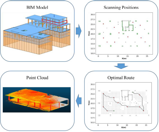
:Scan planning of buildings under construction is a key issue for an efficient assessment of work progress. This work presents an automatic method aimed to determinate the optimal scan positions and the optimal route based on the use of Building Information Models (BIM) and considering data completeness as stopping criteria. The method is considered for a Terrestrial Laser Scanner mounted on a mobile robot following a stop & go procedure. The method starts by extracting floor plans from the BIM model according to the planned construction status, and including geometry and semantics of the building elements considered for construction control. The navigable space is defined from a binary map considering a security distance to building elements. After a grid-based and a triangulation-based distribution are implemented for generating scan position candidates, a visibility analysis is carried out to determine the optimal number and position of scans. The optimal route to visit all scan positions is addressed by using a probabilistic ant colony optimization algorithm. The method has been tested in simulated and real buildings under very dissimilar conditions and structural construction elements. The two approaches for generating scan position candidates are evaluated and results show the triangulation-based distribution as the more efficient approach in terms of processing and acquisition time, especially for large-scale buildings.
1. Introduction
The evolution of sensor technology in recent decades has made possible the acquisition of 3D data in an accurate and quick way. This has stimulated interest in its use in different fields, especially in Architecture, Engineering and Construction (AEC). Within these disciplines, Image-Based and Time-of-Flight-Based technologies have been the two major technologies used to acquire spatial data [1].
Light Detection and Ranging (LiDAR) sensors such as both Terrestrial and Mobile Laser Scanners (TLS and MLS) provide highly accurate geometric data in point cloud format. While data acquisition process by TLS is statically realized from specific locations, MLS dynamically captures spatial data along a trajectory [2]. Increasing 3D spatial acquisitions with LiDAR devices has raised an interest in automated processing of point clouds in researchers of remote sensing, computer vision and robotic communities.
The availability of geometric information of the construction elements "as is" with high accuracy has motivated the use of TLS in the construction industry. This information, known as as-built data, is of great value for construction site monitoring [3]. Traditionally, the assessment of construction elements was done manually—both the data collection process and the data review process—that meant to inaccurate and error-prone evaluations. Since the 2000s, several researchers have pointed to the need to automate the processes of monitoring and control of the progress of the construction in order to overcome the inaccuracies of manual methods [4,5]. In line with this, some methods have been proposed [6,7].
While TLS provides accurate 3D data, in many instances planned drawings consist of 2D plans that makes the quality control of constructed building elements difficult. Fortunately, the growing use of Building Information Models (BIM) makes 3D drawings available [8], and what is more important, the organization of information according to the planned construction status. Several studies have indicated that the use of BIM technology in construction projects improves the construction quality control process because the availability of BIM models is essential to accurately compare as-designed and as-built building components [9,10].
The increased use of BIM models, together with the use of scanning lasers in civil engineering, has awakened interest in the integration of both in recent decades. Many efforts have focused on the automatic generation of BIM models from 3D point clouds acquired as-built for the purpose of obtaining models of real structural elements with an accuracy of a few millimeters [11]. This technique, coined as scan-to-BIM, continues to be studied in order to optimize the entire process through the development of applications that allow BIM models to be generated automatically and efficiently [12]. However, this technique is not suitable for tracking the progress of construction elements, as the unambiguous identification of objects is not guaranteed. Scan-vs-BIM approach is conceived as the comparison of scan data and BIM model by aligning 3D point clouds in the same coordinate system as the BIM model [13].
Generally, scanning is a time-consuming task, so minimizing the number of scanning operations is essential for efficient scanning planning. In addition, data acquisition must be successful in terms of integrity. Determining the next position in which the scanner should be placed is known as the Next Best View (NBV) problem, and is widely addressed in the areas of 3D recognition and reconstruction of both objects and environments. Usually, scan positions known as viewpoints are calculated beforehand, and then an estimate is made of the parts of the scene that would be acquired from each viewpoint. Many methods have been proposed to solve this problem, most of them without prior knowledge of the scene [14,15]. If data acquisition is done in indoors, 3D scene data can be simplified to 2D map, which implies a significant reduction in computational requirements [16].
In this work, a method to determinate the optimal scan positions and the optimal route followed by a stop & go system based on the use of BIM models, and considering data completeness as stopping criteria, is presented. BIM models are used to extract floor plans according to the planned construction status considered for construction control. The well-known DXF standard containing geometric information of the building elements is used to calculate candidates to scan positions, which are subsequently submitted to a visibility analysis using a ray-tracing algorithm. Next, scan positions are optimized based on visibility and data completeness as stopping criteria, and a probabilistic ant colony optimization algorithm is implemented to obtain a suboptimal route in a reasonable time. The output data of the algorithm is used by a robotic unit, where a TLS is mounted, to conduct an autonomous building acquisition. This work specifically addresses the following specific objectives:
- To compare two methods of scan position distribution (grid-based and triangular-based) and select the one that shows the most robust behavior.
- To design a method adapted to the building complexity.
- To consider acquiring vertical elements, such as beams, from a two-dimensional perspective.
- To implement a route calculation and optimization method that joins scan positions avoiding obstacles.
The remainder of the document is structured as follows. Section 2 collects the work related to the problems present in our method which is described in Section 3. The experiments and results shown in Section 4 demonstrate the applicability of the method. Finally, Section 5 is dedicated to concluding the work.
2. Related Work
This section deals with the review of the recent literature on scan planning in indoor environments mostly for control of execution, followed by a review of methodologies addressing the distribution of the navigable space.
2.1. Scan-Planning in Indoor Environments
The planning of 3D data acquisition task is a typical issue in computer vision. Generally, a sensor is used to collect geometric data of close objects in the environment. The quality of the acquired data is highly dependent on the position where the sensor is located with regard to the target. Hence, determining the best positions to carry out data acquisition is a key issue in scan-planning.
Scan-planning can be classified as model-based or non-model-based whether previous knowledge of the scene is available or not available, respectively [17]. If the scene is previously known, optimal scan positions are selected from the analysis of the scene, so that scan positions are determined before of the scanning process. If the scene is not known, the problem is generally formulated as an NBV (Next Best View) problem by which the next best scan position is determined after each scan, considering just the partially acquired scene.
Several methodologies address scan-planning of buildings assuming previous knowledge of the scene. Although this issue is well-known in computational geometry as the art-gallery-problem, a realistic solution should consider certain properties of both the sensor and the objects to be acquired. A variant of the art-gallery problem, taking into account laser constraints such as range and incidence angle, is proposed by González-Baños [18]. A 2D map composed by polygons representing the navigable space and holes assumed as obstacles influencing visibility. The navigable space is randomly sampled to generate an arbitrary number of candidate positions. Then, a ray-sweep algorithm is proposed to obtain a visibility polygon of every candidate position and the selection of scan positions is approached as a set cover problem. This methodology is extended by including more laser constraints such as the minimum and maximum range and angle [19]. A similar solution is proposed by Soudarissanane et al. [16], but in this case, the navigable space is gridded to generate the candidate positions and the visibility analysis of all positions can be time-consuming when dealing with large facilities. Jia et al. [20] propose a more efficient approach to candidate generation. A coarse grid is used for obtain a first set of positions, their suitability for acquisition is evaluated for a proposed Weighted Greedy Algorithm (WGA). A hierarchical strategy is carried out to densify the network distribution in order to achieve a comprehensive scan of the scene by evaluating the smallest number of candidates. The method is geared to outdoors environments and only walls are considered. Biswas el al. [21] also employ a grid to generate candidate positions. Nevertheless, visibility analysis is carried out in the 3D space and semantic information of building elements is obtained from the input model to direct the capture just to structural elements. The input model is a BIM and the approach is validated in a simple scene with circular columns uniformly distributed. Another recent approach is the one presented by Elzaiady [22] in which polygons are extracted from an occupancy grid map (input). Boundaries of polygons represent surfaces whose geometrical features should be collected by sensor. Occlusions along the line of sight of sensor are taken into account for the visibility analysis but the presence of holes on floors and the occlusions caused by the existence of horizontal structural elements such as beams are not addressed. An approach aimed at scanning planning in large construction environments is proposed by Zhang et al. [23]. Scanning positions are calculated from a set of manually determined input points of interest called point goals. The optimization of process is conducted by a “divide-and-conquer” strategy that groups point goals according to required level of detail (LOD) and visibility. The method is tested and compared with scan plans created by experts in a real case from outside the building.
Almost all model-based approaches provide blanket coverage; in other words, they do not take advantage of semantic information from planned layouts, and more specifically, building horizontal elements such as beams or slabs are not taken into account. This information is relevant to direct the scan acquisition to specific elements, such as, in the case of construction control and execution.
The recent developments in robotics and laser scanner technology have increased the attractiveness for indoor acquisition, especially when scenes are big and traditional acquisition would be very time consuming, and also in the case of unsafe environments such as industrial environments and electrical substations. When data collection is conducted autonomously, the scan planning is commonly formulated as the aforementioned NVB problem.
Although most of the recent methods are based on discretizing the space using 3D grids, some methods have proposed the simplification of the problem into the 2D space. Surmann et al. [24] simplify the geometry of a room to a 2D map, where horizontal lines represent walls and are labelled as seen or unseen lines. A polygon is generated connecting seen lines and the navigable space is determined by the boundaries of the polygon. Candidate positions are randomly generated and evaluated by laser beam simulation varying incidence angle. Strand et al. [25] propose an approach also based on projecting 3D data to a 2D map. In this case, each cell of the map has information about occupancy. Empty cells are considered as candidate positions and a simulation of the laser beam is performed from each of them.
The concept of a 3D occupancy map has been highly explored to solve the NBV problem. Potthast et al. [26] propose a method based on observation probability. Using a ray-tracing algorithm, the observation probability of each cell is assigned according to Markovian observability. The method is tested in real case studies and large virtual cluttered environments.
In contrast to the previous work in which a binary map is generated, Adán et al. [27] label the space into occupied, empty and occluded units. For this purpose, the scene is voxelized and ceiling and floor are extracted to determine the boundary of scene. Next, a ray-tracing algorithm is implemented to label the voxels into occupied, empty and occluded. Next, the voxel space is projected to a 2D image with labelled pixels, and the next scanning position corresponds to the empty pixel from which the largest number of occluded pixels are observable. Quintana et al. [28] extend the previous work in a way that the NBV problem is devoted to completing the acquisition of building structural elements, and consequently, floors, walls, columns and ceilings are recognized in successive scans. Prieto el al. [29] also consider the automatic 3D scanning of walls, ceilings and floors in furnished buildings. The accumulated spatial data is registered using an ICP (Iterative Closest Point) algorithm, and an obstacle map is constructed. Voxels are classified and evaluated by probabilistic decision function from a set of candidate positions within the obstacle map. The next scan position is chosen according to the probabilities calculated in the previous step. González-de Santos et al. [30] extend previous approaches to also consider windows and doors, which are identified through a visibility analysis. In this way, once acquisition is completed for one room, the existence of doors determines subsequent next best scans.
With regard to previous approaches, this work focuses on the selection of optimal scan positions and the calculation of the optimal route that connects them. Since the method uses a BIM as input, the environment and the types of elements that compose it are known. The authors have opted for a 2D approach for two reasons: the TLS is positioned at a fixed height in the robotic unit, and processing time is improved by eliminating one spatial dimension. Route planning is typically ignored in scan-planning approaches. In this work, a probabilistic ant colony optimization algorithm is implemented considering the building geometry. The subsequent registration process between scans is not part of the present work, although it has been considered an option to place scanning positions on the doors to facilitate the overlap between scans. The method is tested in real and complex scenarios with satisfactory results.
2.2. Discretization of the Navigable Space
Scan planning requires an initial evaluation of accessibility to scan positions for the acquisition system. To accomplish this, the knowledge of space through which the system can move free of collisions is essential. The distribution, structuration or discretization of this space, commonly defined as navigable space, is a key process in scan planning. The challenge of this process comes from the continuous nature of the navigable space and the influence of the result on the computational cost of subsequent steps, especially in complex scenes. The discretization of the navigable space should be carried out in a way that it is represented by the minimum number of units satisfying the accuracy required by the application. Detailed reviews of how indoor space can be represented have already been published in recent years [31,32].
The simplest representation of an indoor navigable space is the adopted by standards such as IndoorGML to depict the connectivity relations between rooms. One node represents one room and topology between rooms is represented by using the dual graph [33]. However, this representation is often too simple to be representative of a real path, especially for large scenes [34].
Methods based on Medial-Axis-Transformation (MAT) are used frequently to represent indoor environments (rooms, corridors, etc.) in order to stablish topological relations between spaces [35,36]. Lee [35] proposes a MAT-based method for generating skeleton structures of simple polygons from geometric information only; the algorithm was named Straight-MAT. Another approach based on centerline algorithm and considering previous semantic knowledge is used by Meijers et al. [36] to represent corridors.
In contrast to previous methods, grid-based representations provide a dense and uniform structuration of the navigable space [37]. However, the trade-off between resolution and computational effort is an inherent issue in regular grid techniques. A fine-grained grid entails a high consumption of computational resources especially in the processing of large environments models [31].
Due to their simplicity, grid-based representations are widely used in robotics for the creation of occupancy maps. These representations can be addressed from a 2D [38,39,40] or 3D [41] point of view. For example, Li et al. [40] structure the navigable space as 2D squared cells represented by one node and identified by an attribute according to the building element they represent. Bemmelen et al. [38] extend the latter structure adding nodes at sides of squares with the goal to enable more directions between adjacent cells during space navigation. Joo et al. [42] generate a topological grid-map by means door detection from grid occupancy map. Equivalent three-dimensional grid discretization is known in literature as “voxelization” and the unit basic of this structure is a voxel.
To enhance efficiency of operations with high density grid representations, hierarchical-organization structures such as quadtrees [42] and octrees [43,44] are commonly employed in 2D and 3D spaces respectively. Detailed representation is obtained by means of the recursive subdivision of cells or voxels.
Voronoi diagrams are also one of the most fundamental data structures in computational geometry [45]. The plane is partitioned in polygonal regions called Voronoi regions from a set of points. The generalization of Voronoi Diagrams (VD) allows the space partition not only from a set of points but also from line segments [45]. Based on VD, Wallgrün [46] proposes a hierarchical network graph for mobile robot navigation. Vertex of Voronoi Diagram are labelled with information of distance and angles related to seed points that correspond to obstacles boundaries. Length of edges and relative position of nodes are also taken into account. Next, this information is used to determinate the relevance of each vertex in the navigational network.
Boguslawski et al. [47] use VD to create the proposed Variable Density Network (VDN). First, each subspace (such as rooms and corridors) is represented by a cell and abstracted as a node. Adjacency of subspaces is represented by linking their respective nodes with an edge. Then, VD is generated from door nodes and concave corners of the previous structure. An iterative process of re-densification is carried out considering two arbitrary parameters. New points are added to the original VD for those cases in which segments are longer than a certain threshold. The number of iterations is limited.
Many navigational approaches are based on a dual representation of VD known as Delaunay Triangulation (DT). This technique consists in the union of initial sites of adjacent Voronoi regions generating a partition composed of triangles. In navigational network construction it is common to impose restrictions to the segments that form the triangles, this variant of the method is called Constrained Delaunay Triangulation (CDT). Lamarche et al. [48] structure virtual complex environments into convex cells applying a two-step division process. First, narrowness in navigable space are detected by using a modified CDT. Then, resulting space division is simplified grouping triangles into convex cells.
Space navigable division is also carried out in two phases by Krūminaitė et al. [49]. In the first stage, the space is classified as navigable and non-navigable according to previously defined patterns of human behavior. The second step consists of the division of navigable space by means a CTD. Centroids of triangles obtained in the previous step are calculated and joined to design a navigation network.
A recent method considers a classified point cloud as a model itself for navigational purposes [50]. Segments of point clouds corresponding to floor elements, previously classified as ramps, steps, etc., are downsampled, considering a minimum distance between points, and resulting points are considered the nodes of the navigational graph [49].
With regard to previous approaches, it has been observed that the grid-based algorithm presents an unwanted behavior in large and complex floor plans. For this reason, together with the grid-base method, a triangulation-based method has been implemented to give the end user the option to choose the most appropriate distribution for their case study. Both methods have been compared in terms of density and distribution of scan positions, which is a critical issue in large and complex scenes. When delimiting the navigable and accessible space by the robotic unit, its parameters have been considered in order to delimit these spaces correctly.
3. Methodology
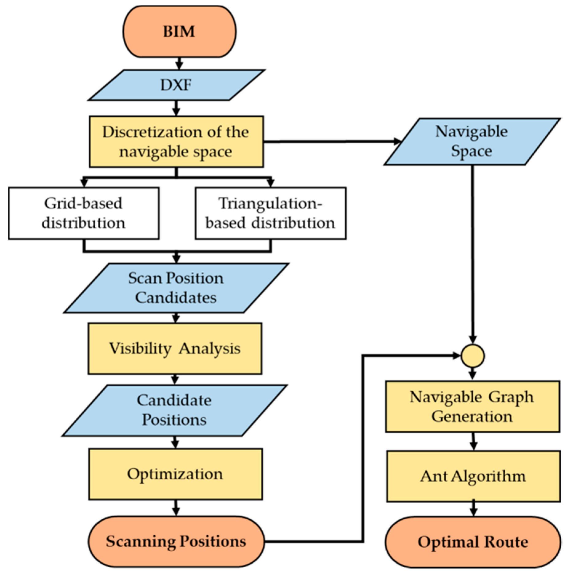
The general workflow of the method is represented in Figure 1. The input of the method is a BIM model in which building information is managed according to an execution plan, and outputs are the optimal scan positions and the optimal route for visiting all scan positions once.
3.1. From 3D to 2D
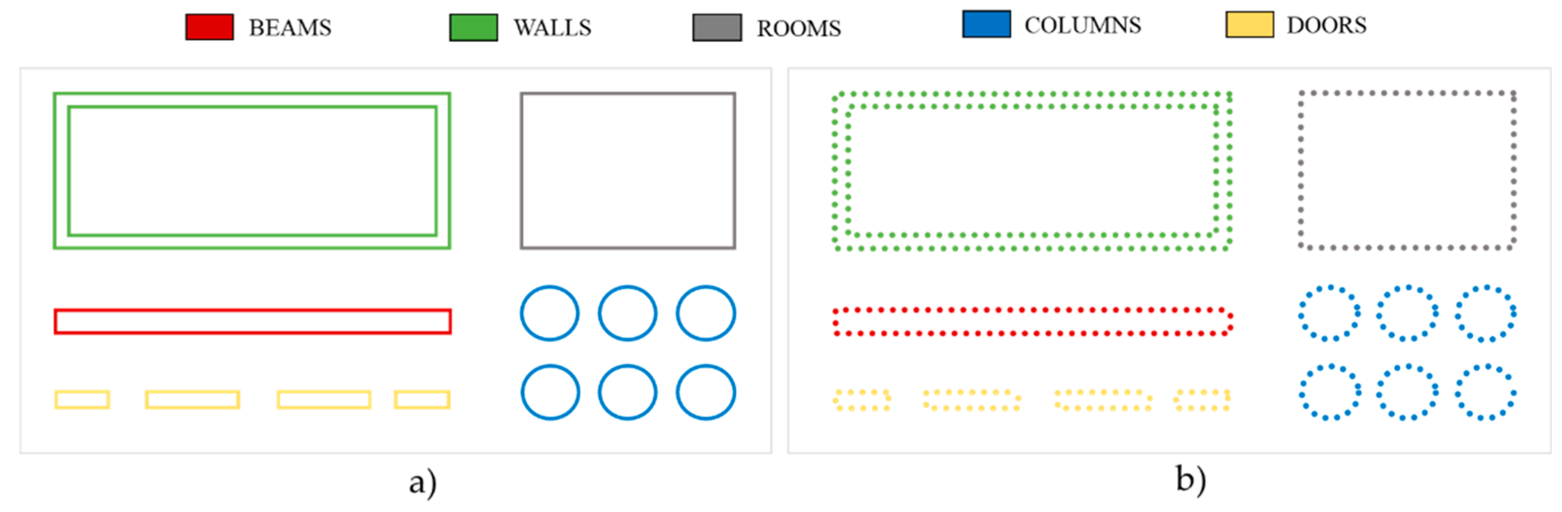
As this method is planned for large-scale buildings, 3D BIM elements are converted to a 2D plane in order to lighten computational effort [16]. Scan process is planned for an acquisition system considering the plane XY. For this purpose, BIM elements are exported to DXF according to the planned construction status that is considered for control of execution. Semantic information regarding the nature of the building elements is preserved as layer names, what enables the direct acquisition process to relevant elements. Then, geometric elements referred as entities in CAD (i.e., lines, polygons, arcs and circles) are discretized as equidistant points E to be used for further steps (Figure 2).
In the case of linear elements represented by vertices, such as lines and polygons, the number of points E of each straight line is determined as the minimum number of segments of length ddis needed to represent the entire line. In elements represented geometrically by a central point and radius, such as circles and arcs, the discretization points E are generated according to the angular resolution defined by the following equation:
3.2. Discretization of the Navigable Space
The space through which the acquisition system can move free of collisions is considered as the navigable space. Consequently, it can be easily defined by the boundary of floors, considering the space occupied by vertical building elements and a security distance dsec determined by the robotic unit dimensions. The distance dsec is defined by the user as the minimal distance between central point of the platform and the nearest obstacle. In case of rooms connected by doors, the door width must ensure accessibility.
The continuous nature of the navigable space requires a discretization in a way that is it distributed into candidate scan positions, known as those theoretical places, in which the scan can be placed. The number of scan positions highly influences the computational cost of the process. Therefore, discretization should be performed in a way that navigable space is correctly represented by the minimum number of points.
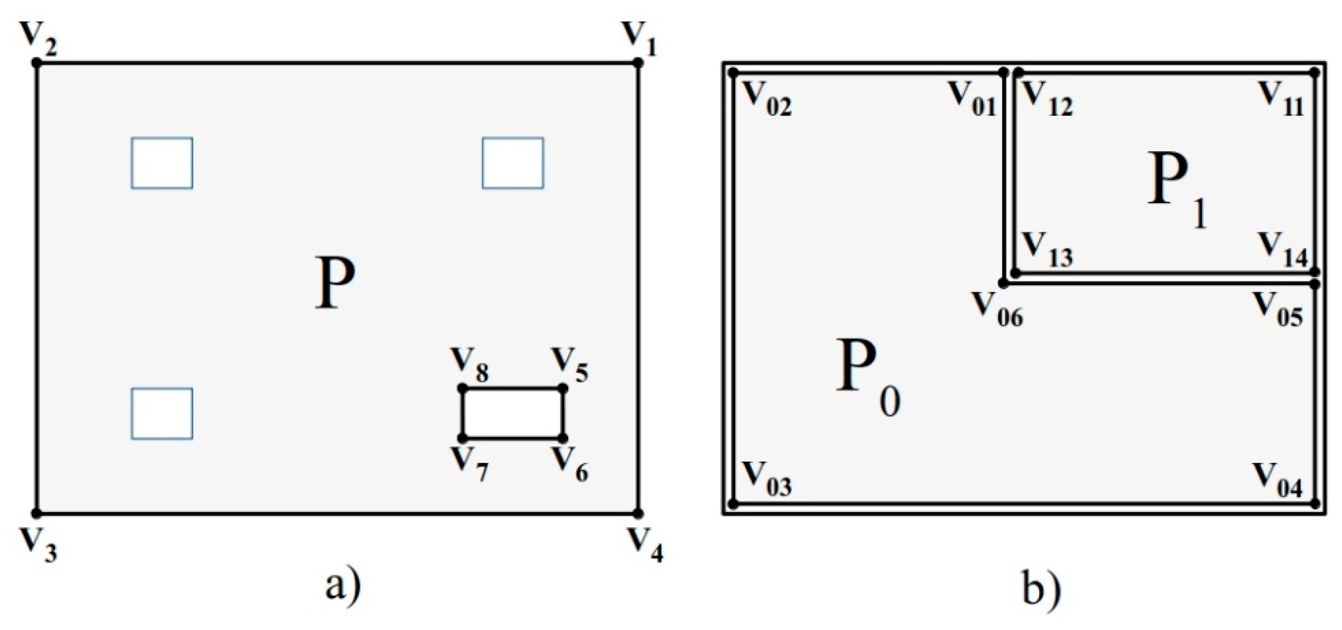
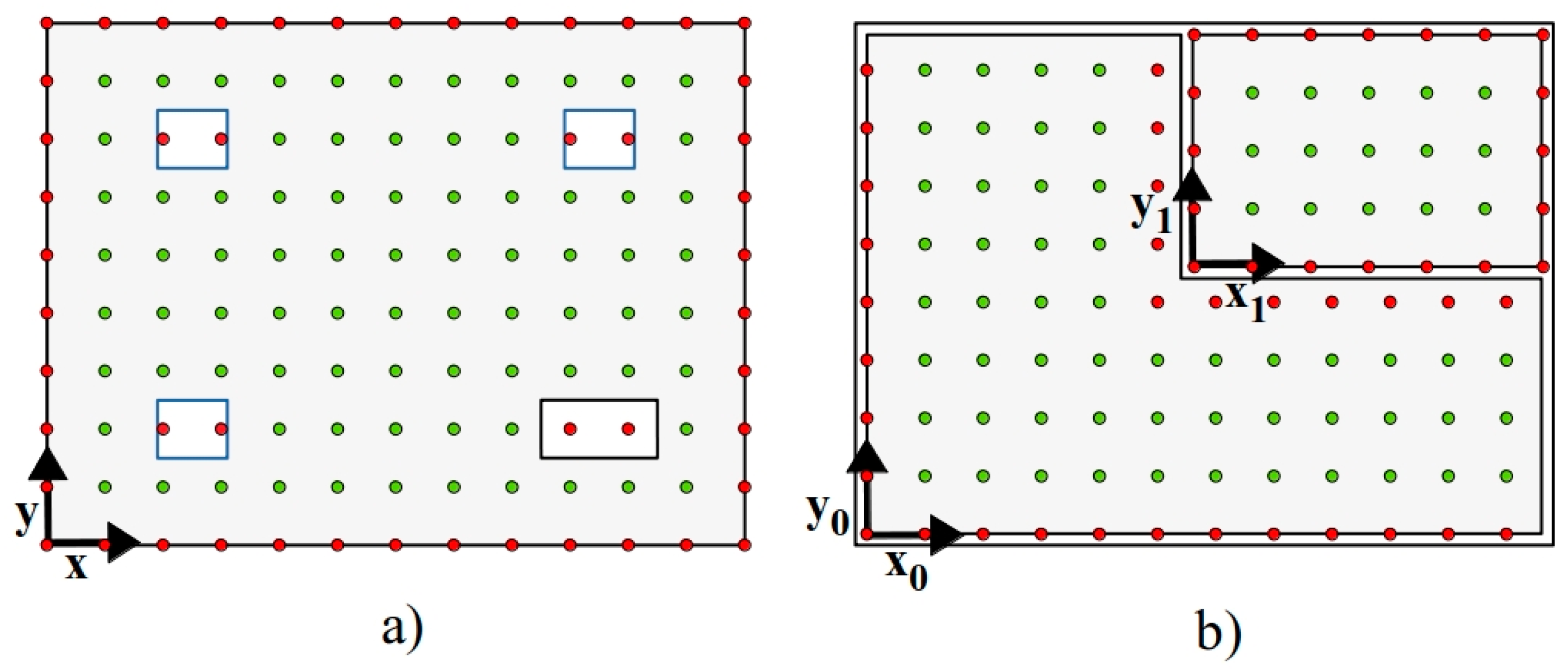
Contour of the navigable space is represented as the boundaries of a polygon P (Figure 3a). Polygons are defined by a set of vertices organized in counterclockwise direction V = {v1, …, vn}. In case of the existence of holes in the navigable space, vertices are defined clockwise. This representation is typical from early stages of the construction process in which rooms are not still constructed, and holes are caused by the planning of stairs, elevators, pipes, etc. If rooms are represented, P is decomposed in smaller navigable polygons Pn (Figure 3b). This subdivision only indicates when constructed walls separate different spaces. In which case, polygons define navigable space P = {P0, …, Pr}, where Pi with i = 0, …, r corresponds to the polygon that represents the room i. As well as P, each Pi can be defined by its vertices Vi = {Vi1, …, Vim}, where m is the number of vertices each room/corridor.
3.2.1. Grid-Based Distribution
The implemented grid-based method consists in a regular tessellation that provides a partition of the space in regular squared cells Pn (Figure 4a). If rooms Pn are represented in the DXF, the space partition is carried out separately by each room. A local coordinate system is adopted to distribute the candidate scan positions and grid resolution is adjusted to room size (Figure 4b).
The vertices of cells Vc, that compose the grid constitute the candidate positions Scand = Vc. Grid-based methods yield uniform and dense space divisions. However, the size of candidate positions obtained from this distribution may involve higher computational costs, especially in larger scenes. The existence of holes H and a security distance dsec defined by the robotic unit are used for filtering final candidate scan positions and , those in which the system can be placed to perform acquisition (Figure 4).
3.2.2. Triangulation-Based Distribution
Complex floorplans usually require high-density grids, but the analysis is very time consuming. In order to overcome the limitations of grid-based distribution, a triangulation distribution based on the well-known Delaunay Triangulation is implemented (Figure 5).
Before applied Delaunay Triangulation, seed points Se are necessary to generate a Voronoi diagram. Vertices V of lines defining building elements (i.e., walls) and centers of circles C (i.e., circular cross-section columns) are used as seed points for Voronoi process . In case the distance between input points is higher than dmax, new seed points Se are generated. The Euclidean distance d of each segment is calculated and compared with a distance dmax. Segments d > dmax are split generating new evenly spaced points. Figure 6 shows a schema of the seed generation approach. In the case of an early stage of the construction, in which the floor plan is not divided into rooms, floor contour vertices and column centers are considered as seed points. In the case of an indoor scene divided into rooms Pi, each room is individually processed, analogue to Section 3.2.1. In the Voronoi process, new seed Si points in the interior of the room are generated. Se and Si are used as input for the discretization process based on a Delaunay Triangulation. This step is essential for a good distribution of candidate scan positions, especially in big rooms with simple geometry.
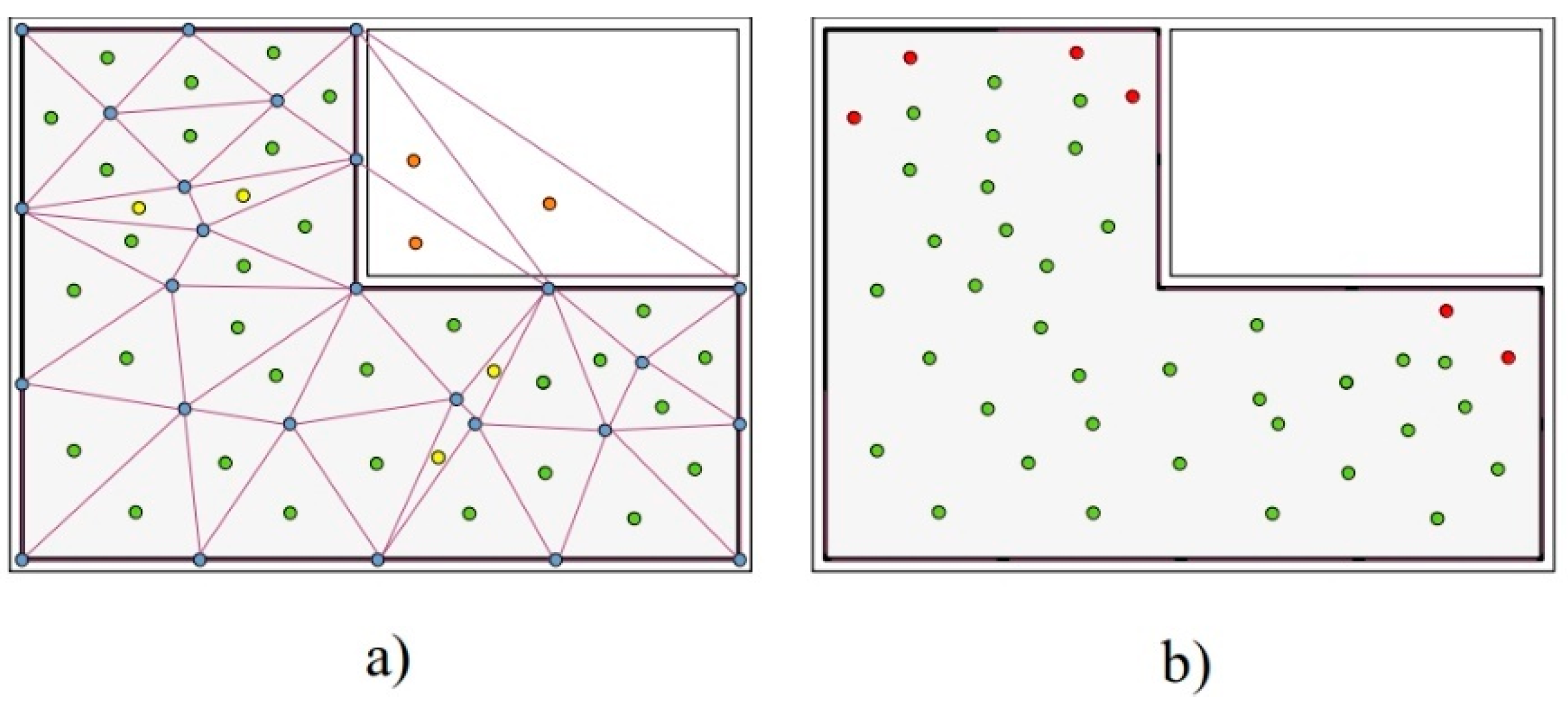
Once seed points {Se, Si} are obtained and Delaunay Triangulation is implemented, candidates to scan positions Scand are filtered in order to discard those candidates out of the navigable space or representing low-interest areas (Figure 7). In the first case, triangles whose centroid are outside of the navigable space are removed from the selection. This happens mainly in concave spaces. In the second case, triangles with very small angles and sides are discarded considering by angle αmin Equation (2), being the minor side of the triangle. Also, the candidate positions must fulfil with the constrains of dimension and mobility of the robotic unit.
One weaknesses of candidate position generation by using a triangulation method is that the density of candidate positions may be insufficient to provide a good coverage. Density is defined as the ratio between the number candidate positions Scand and the polygon area containing them. In order to ensure an acceptable density, triangulation is iterated for those rooms with density inferior to densmin, generating new candidates.
3.3. Visibility Analysis
In order to evaluate the suitability of each candidate scan position and to determinate the coverage of the scene, a visibility analysis is performed for all candidates Scand. This process is based on a ray tracing algorithm that simulates the laser beam and establishes the surface theoretically acquired by a laser scanner taking into account scanner range r and field of view v.
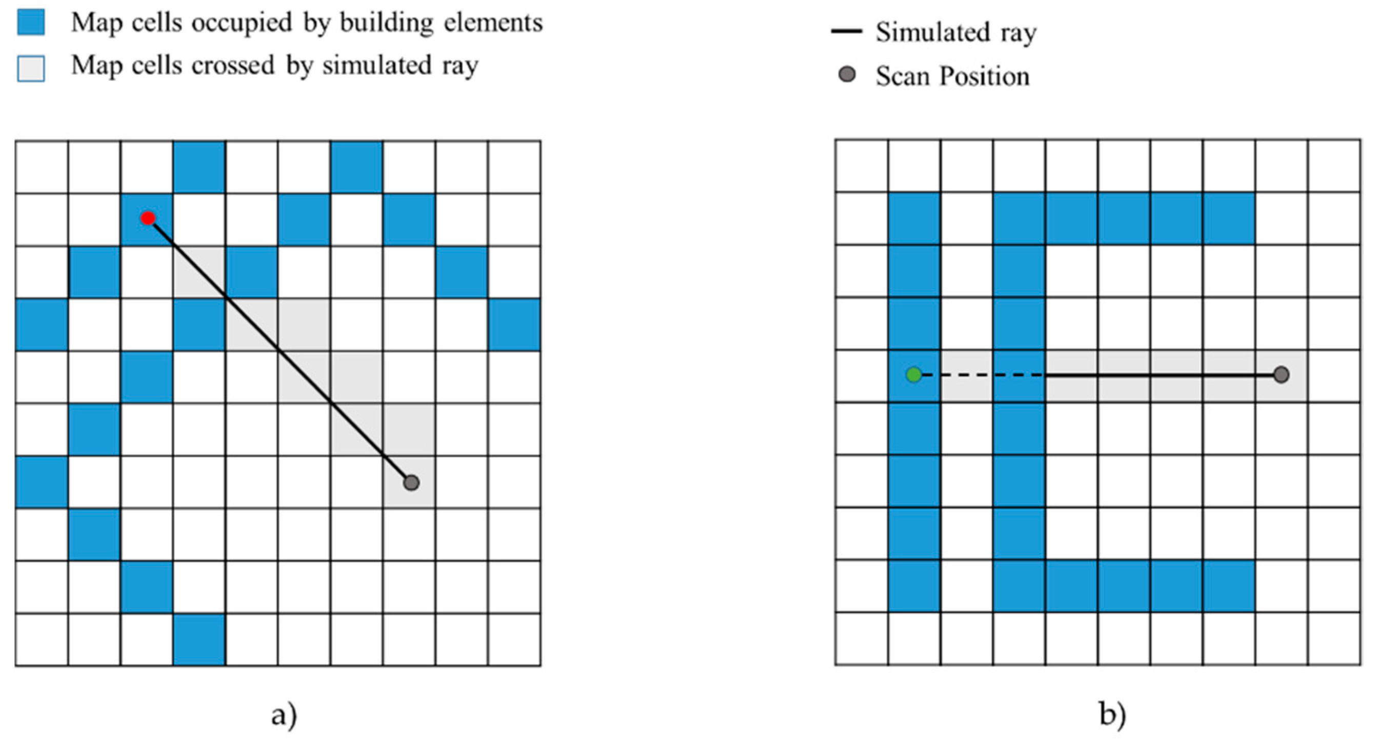
For this purpose, the implemented method (Figure 8a) is similar to Diaz-Vilariño et al. [51]. Candidate positions are located in a binary occupancy map I = (Ix,Iy). Then, the cells crossed by rays simulated between laser position and target cells (all cells in the field of view and range of the laser) are calculated by Bresenham´s line algorithm [52]. After this step, visible cells for each candidate to scan position are obtained Iv.
Visibility analysis by Bresenham´s line algorithm can lead to errors in visibility estimation when vertical elements are not perpendicularly aligned with X and Y axes in a Cartesian Coordinate System (Figure 8b). For this reason, the DXF plane must be rotated to align principal elements with XY axes.
3.4. Scan Optimization
Once visibility analysis is completed, theoretical visible surfaces from each candidate position are known. If the distribution of candidates is robust in terms of coverage, building elements are visible from different candidate positions.
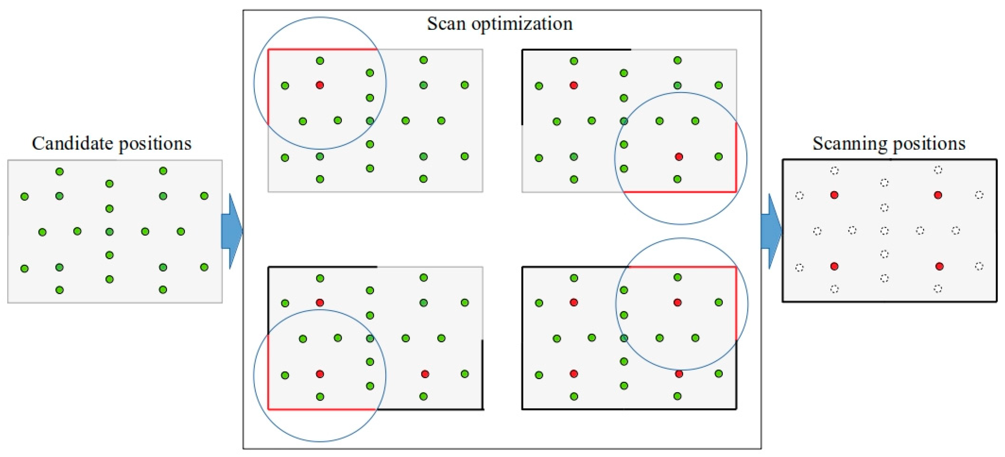
Since the goal of this method is to obtain the minimum number of scanning positions Sscan for avoiding the acquisition of repetitive data, an optimization is performed by using a backtracking algorithm [53]. Final scan positions are determined considering the theoretical surface acquirable a from each position (Figure 9). The best scan position is the one from which a larger number of cells are visible. The rest of the scan positions are being selected based on the number of visible cells that can provide to the already selected positions . The process is repeated until a minimum of coverage cmin is accomplished (stopping criteria). Since semantic information is preserved from the BIM model, scan optimization can be directed to the control of specific elements in the scene.
3.5. Optimal Routing
Unlike most scan-planning approaches, the calculation of an optimal route for scanning position is tackled. This problem can be raised as the well-known travelling salesman problem (TSP) that is formulated as: given n cities identified by its positions, to determine a path so that all cities are visited just once, travelling as little distance as possible. This problem is framed within the NP-hard complexity problems, wherefore the optimal solution cannot be obtained in a reasonable time. Typically, the problem is solved by means heuristic approaches that conduct sub-optimal solutions within a reasonable time. This work implements a probabilistic algorithm based on the ant colony algorithm family [54]. This algorithm is based on modelling the behavior observed in real ants to find short paths between food sources and their nest. The result is an emergent behavior caused from each ant’s preference to follow trail pheromones deposited by other ants.
In order to obtain the optimal route, distances between pairs of scan positions Sscan have to be obtained, and for this purpose, a navigable graph G = {N,E} is created. As grid-based graphs are more suitable for route calculation than triangulation-based graphs [31], the construction of the navigable graph is based on a regular grid.
First, the navigable space is gridded. Vertices of grid cells Vc correspond to graph nodes N. Adjacency between nodes is studied to create the adjacency matrix. Nodes are 8-connected [55] forming edges E. Then, the accessibility of the edges is checked (Figure 10a). Edges crossed by any non-navigable cell are removed. The location of scanning positions Sscan may not coincide with the location of navigable nodes N, previously calculated because this process is independent of candidate generation. In this case, scan positions are relocated to the nearest navigable nodes in order to calculate the optimal route (Figure 10b). In this way, accessibility is ensured.
Once the navigable graph is created, the shortest path P = {Np,Ep} between each pair of scan positions is calculated using Dijkstra algorithm [56]. This information is used to create a simplified graph in which just nodes representing scan positions and distances between them are represented (Figure 11). This simplified graph Gs = {Ns,Es} is used to implement the Ant colony optimization algorithm for obtaining the optimal path.
When navigable space is divided into rooms, a navigable graph is generated for each of them. The scanning nodes are determined in the same way as explained above. Due to graph disconnection, the optimal route calculation cannot be addressed with a global approach of the space. Accessible door positions D are considered as connection nodes between rooms (Figure 12).
From room polygonal representation by using simple polygons arises a particular issue: when there are rooms within other rooms. In this case, the navigable space of inner room must be subtracted from outer room space. Doors between both rooms are considered as doors of the exterior room, even though boundaries do not belong to its contour.
4. Results and Discussion
This section is organized in three sub-sections. The first section presents the data and instrument employed for testing the described method. The second section collects the results obtained and the discussion of them. The third section shows the applicability of the proposed method in a real scenario of an under-construction building.
4.1. Instruments and Data
The method described in this paper has been tested in several cases study, some of them provided by the International Society for Photogrammetry and Remote Sensing (ISPRS) Benchmark on Indoor Modelling [57]. Previous results have been already published in [51].
The developed method is focused on an acquisition system composed by a TLS mounted on top of an autonomous mobile robot. The TLS employed is FARO Focus3D X 330 [57]. The operating mode of the acquisition system follows a strategy known as stop & go. Robot moves to next scanning position, stop at this one and then laser scanner realized the acquisition task. This operation is repeated until all scanning positions are reached by mobile robot. The local planning of robot mobile is out of the framework of this work.
4.2. Results
4.2.1. Parameters and Values
In order to apply the method and guarantee reproducibility, parameters and values are summarized in Table 1. General parameters are required in any case while specific parameters are necessary depending on the scenario and the distribution method. For the comparison of decomposition space methods, the values do not vary in all tests. Some results obtained with different parameters are showed to assess their influence.
The coverage degree cmin is given by the ratio of theoretical area that must be acquired from all visible area of interest. The cmin parameter supposes the stop criterion in the selection of the best scanning positions. The process ends when the ratio of structural acquired elements is greater than or equal to cmin.
4.2.2. From 3D to 2D
BIM models are exported to 2D CAD model with DXF format. The Figure 13 shows (a) the BIM model and (b) and (c) the 2D models—case studies—extracted from the BIM model of the case studies. For each case study, two virtual scenarios have been proposed. On one hand, a structural stage considering beams and columns for control of execution, and the existence of stairs as elements influencing the visibility. The second scenario is composed by columns, walls, stairs and doors. Rooms are also defined. Beams have been manually created to perform the simulation, since they were not represented in the BIM.
According to input requirements, the entities of the facilities are arranged by layers. The definition of floor layer, which enclose the navigable space, is a preliminary condition. Auxiliary layers, such as rooms or doors, can be used to improve the efficient of the processing.
4.2.3. Distribution of the Navigable Space
The discretization of continuous elements has generated a variable number of units depending on number and size of structural elements. The number of units for res_disc = 50 mm is collected in Table 2.
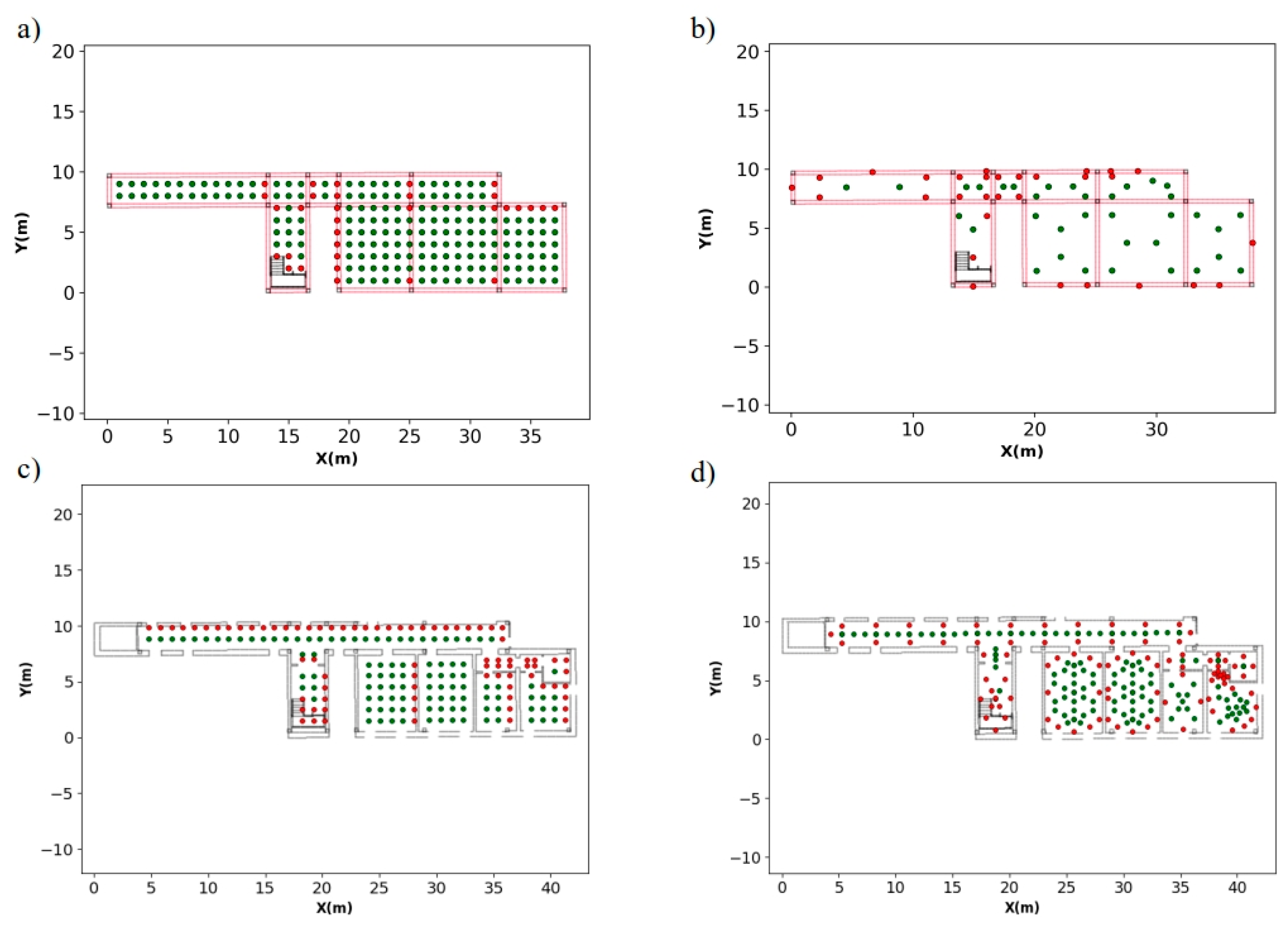
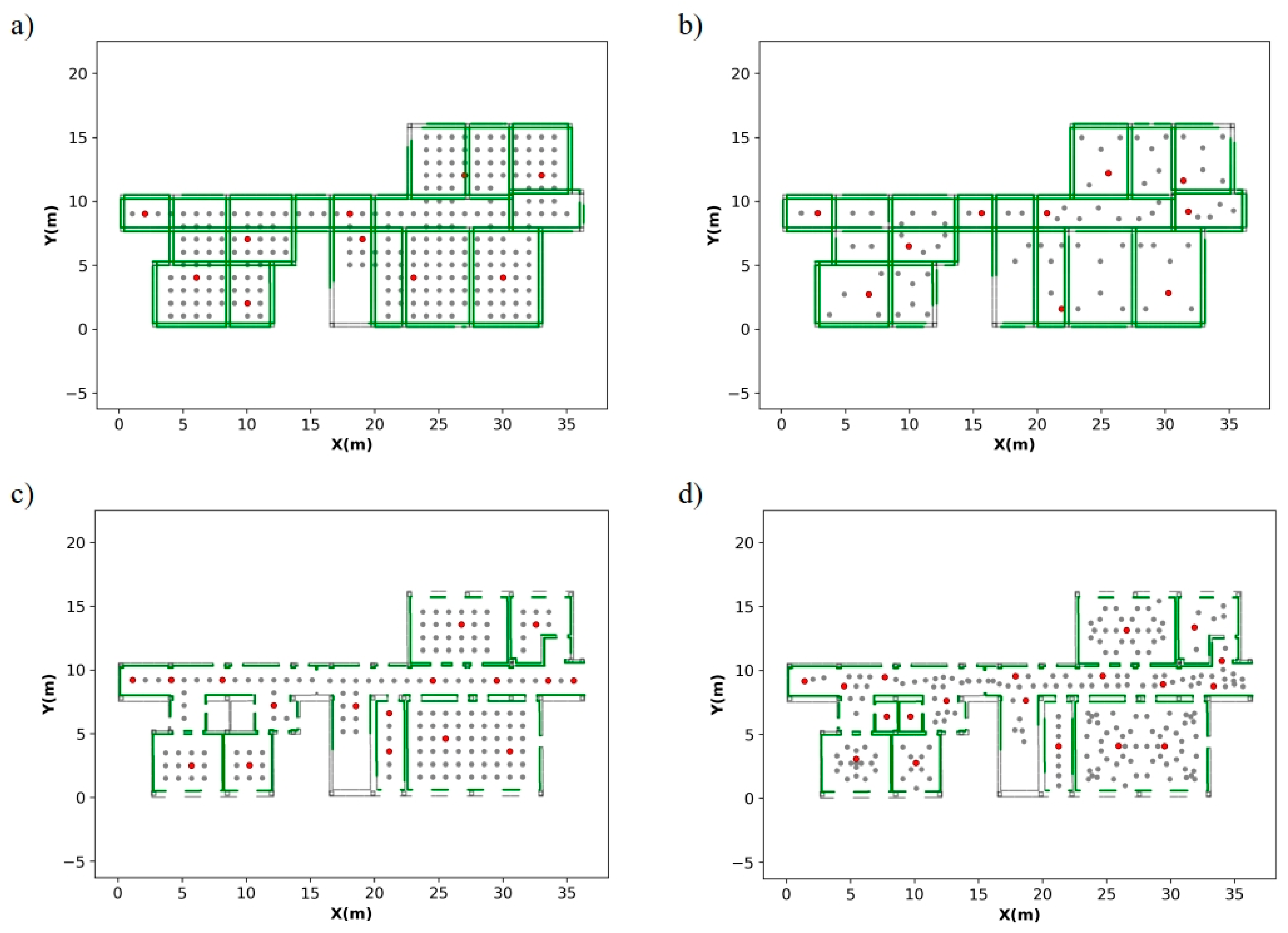
The number of candidate scan positions depends on the discretization method and construction phase. Figure 14 and Figure 15 show candidate scan positions generated by grid-based method and triangulation-based methods of space partition implemented. The results confirm the expected behaviour of both methods, grid-based method led to more regular distribution than triangulation-based method. In structural phase, grid-based method generates more candidates than triangulation. With rooms, triangulation provides more density distributions. The number of scan positions is listed in Table 3.
Based on these results, the implemented triangulation process provides two main advantages respect to grid-based method for scan-planning in indoor environments. Fewer positions in the structural phase reduces the computational cost of testing each candidate. A greater density of positions in presence of walls dividing space into room offers enhancement in terms of coverage. The two smallest rooms (Figure 14 and Figure 15) are only well partitioned with triangulation-distribution.
The processing times of both discretization methods are similar, in most cases, grid-based is slightly faster than triangulation-based. However, the generation of candidate scan positions has less influence in total time than visibility analysis.
4.2.4. Visibility Analysis
Visibility analysis is a critical procedure in terms of time and completeness. Each candidate position is tested, so the number of candidates have repercussions in execution time. Also, the number of discretization units is relevant, although only those within the range of the laser scanner l_rng are analyzed. Completeness in this process is understood as the ratio of visible elements from all candidates. It can be used as a measure to evaluate the distributions obtained.
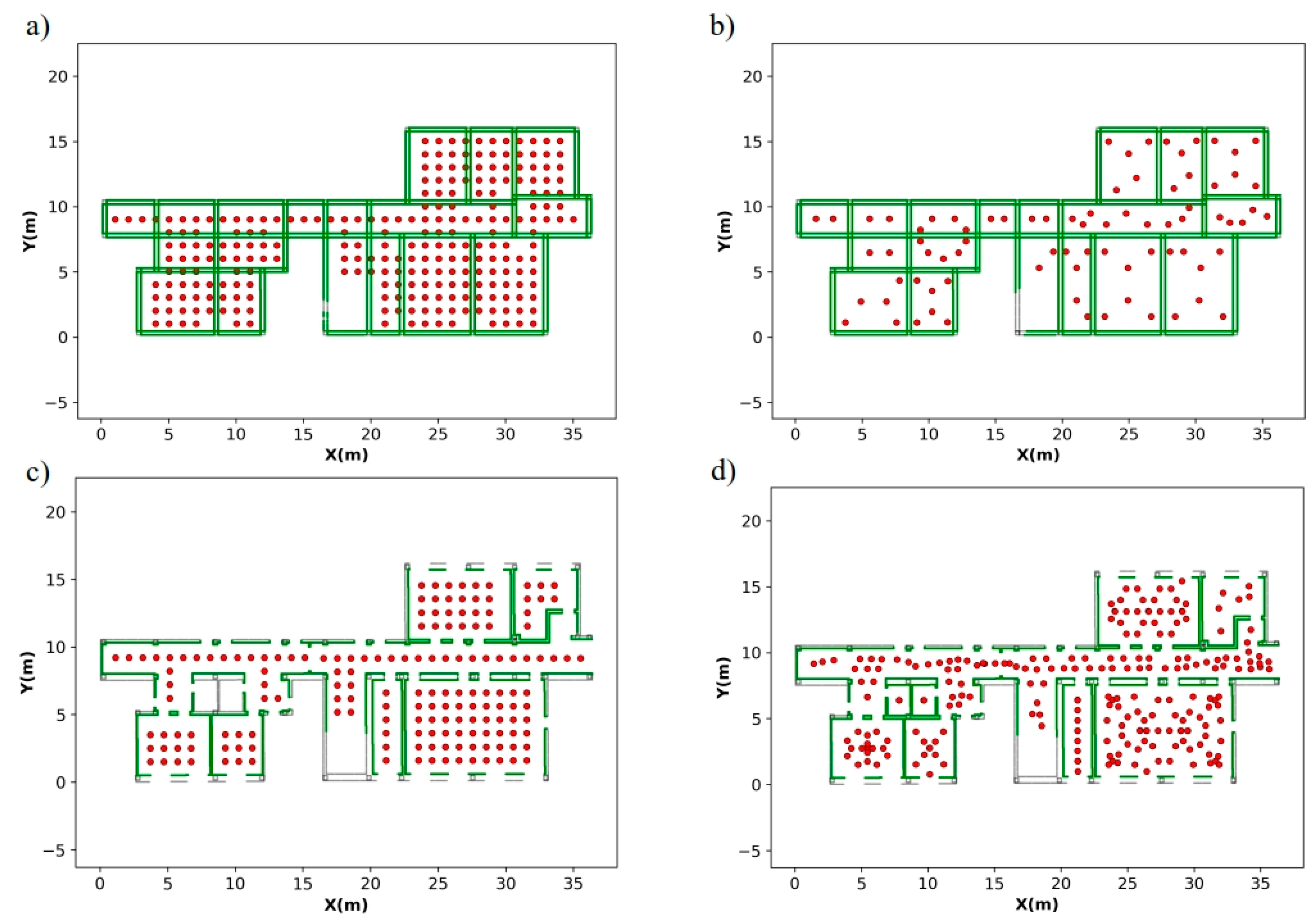
Results of visibility analysis (Figure 16 and Figure 17) conducted in the four case studies are gathered in Table 4. The level completeness is greater for denser distributions. However, this correlation differs depending on discretization-method and construction phase. The grid-based method provides distributions denser than triangulation in structural phase, but the degree of wholeness is not greater. In spaces separated by rooms, triangulation supply a significant better visibility coverage with a decreased density about 40% in the worst case.
With regard to processing time, there is a correlation between the number of candidate positions and the execution time of the process. In contrast to what was observed in the completeness analysis, the processing time seems independent of the partitioning method used. The main relevance, in terms of time, is related to construction phase and is more relevant in structural phase. With rooms, the range of the laser is restricted to rooms. In order to evaluate the influence of laser scanner range, structural phase of case study 1 has been tested with l_rng = 10 m Table 5).
To check the raytracing in the visibility analysis in case studies not aligned with the XY axes of Cartesian Coordinates, case study 1 has been rotated 45º on the Z axis. The visibility analysis on case study 1 rotated is shown in Figure 18. In most of areas of the scene, the behaviour of the algorithm is right except in the framed area because the external wall is considered as visible (double green line).
4.2.5. Scan Optimization
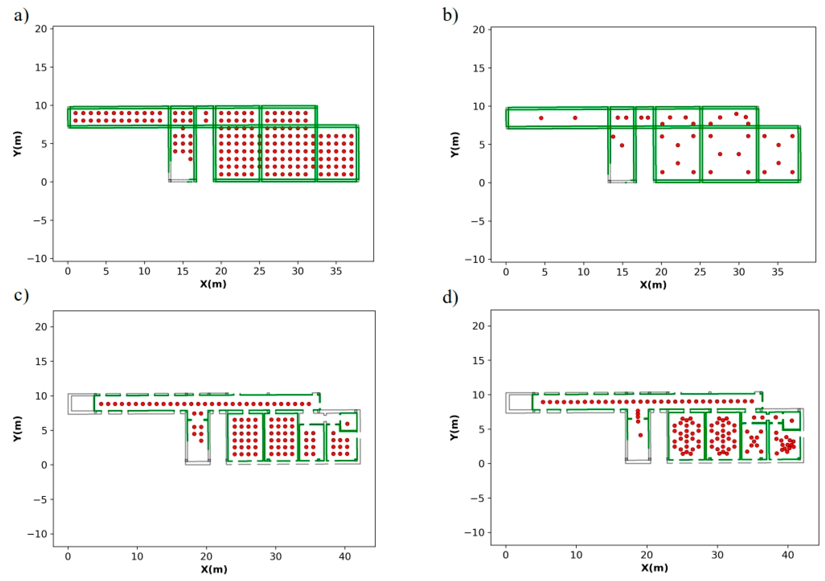
Table 6 shows that the number of selected positions is similar between both discretization methods. The time consumed by the optimization process depends on the number of candidate scan positions. The result of this process is shown in Figure 19 and Figure 20. For the selection of optimal positions, laser constraints, such as incidence angle, density or overlapping, are not regarded. This could compromise the quality of acquired data and cause problems in further registration. As this work is framed in indoor acquisition, short laser range is employed (5–10 m) therefore the effect of angle of incidence is minor [58]. Despite the fact that overlapping is not taken into account during optimization, door_scan parameter enables door locations can be used as scanning positions in order to provide the registration task. Doors locations are added after optimization and they have no influence in scan optimization process.
4.2.6. Optimal Route
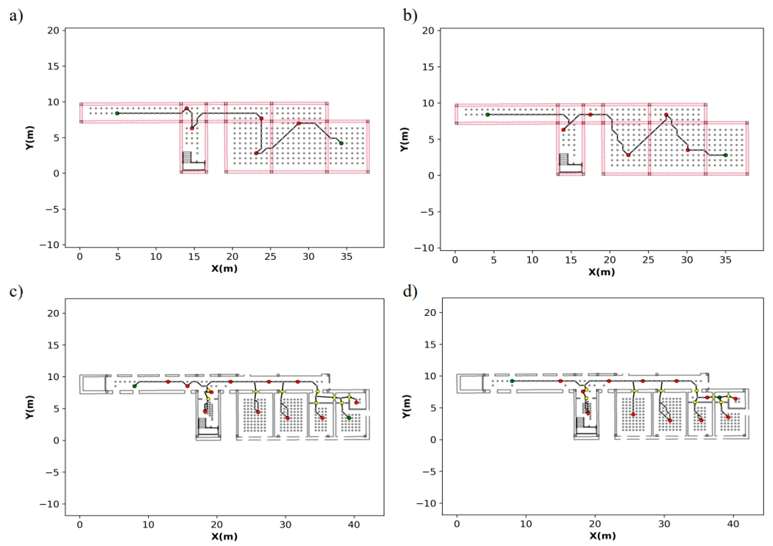
The initial grid resolution is 1 m and the algorithm automatically reduces it until satisfied den_grid_min and max_err_dist. The density of the node distribution is not uniform because a subgraph is calculated for each room individually. Table 7 lists the processing times for the network creation, the route calculation and the route distance. Optimal route is obtained from navigable network by applying ant algorithm. Figure 21 and Figure 22 show calculated optimal routes for the case of study 1 and 2, respectively. As expected, total distance is in accordance with vertical elements of the navigable space and not with candidate generation process.
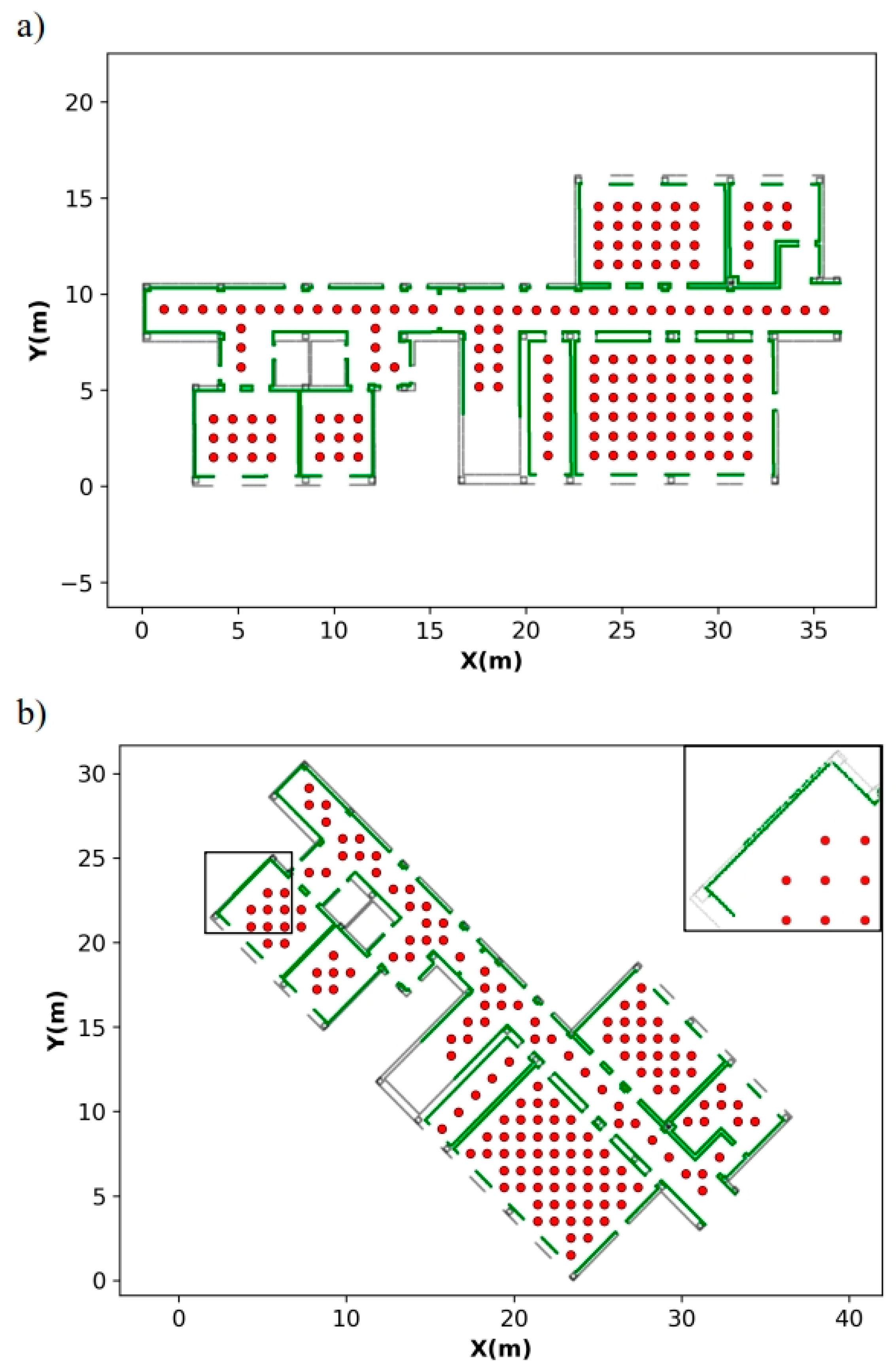
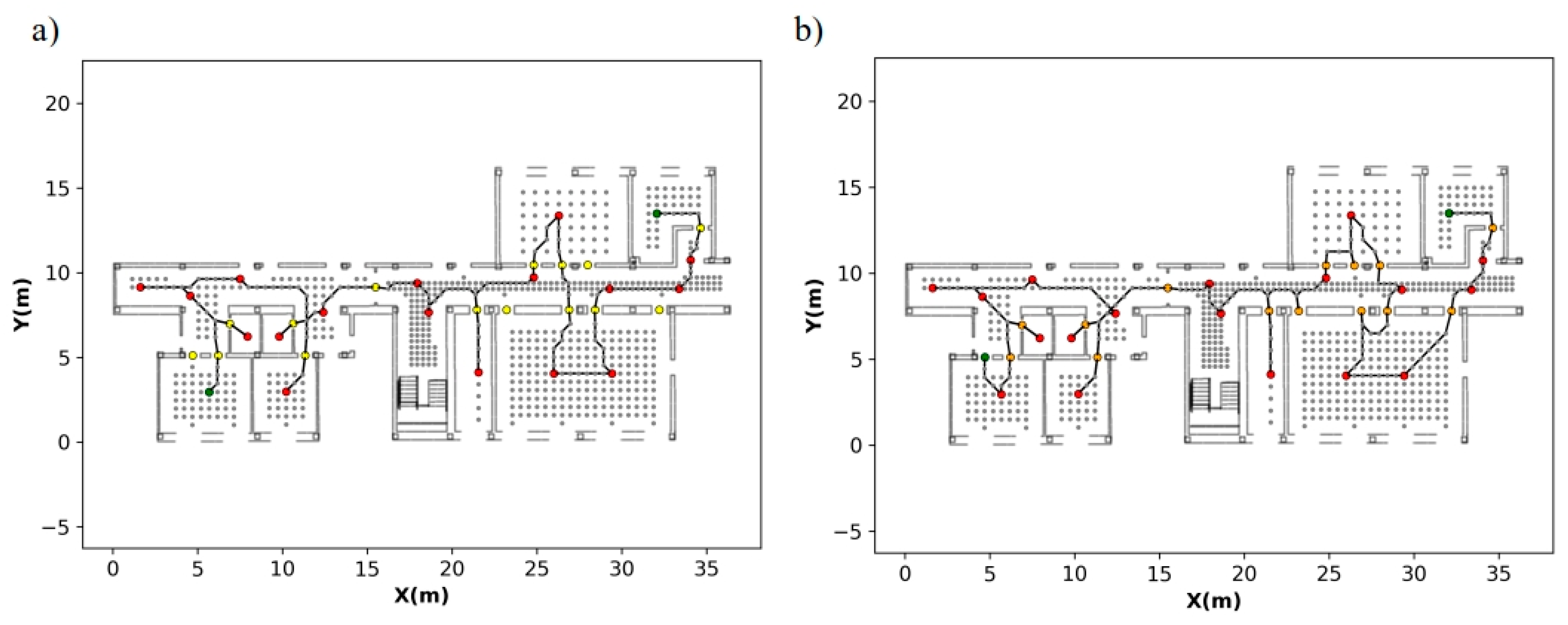
In order to avoid subsequent overlapping problems in registration, door positions can be added to route calculation. Figure 23 shows that the optimal route with door positions is not much longer than the route with only optimal scanning positions.
4.3. Application in A Real Case Study
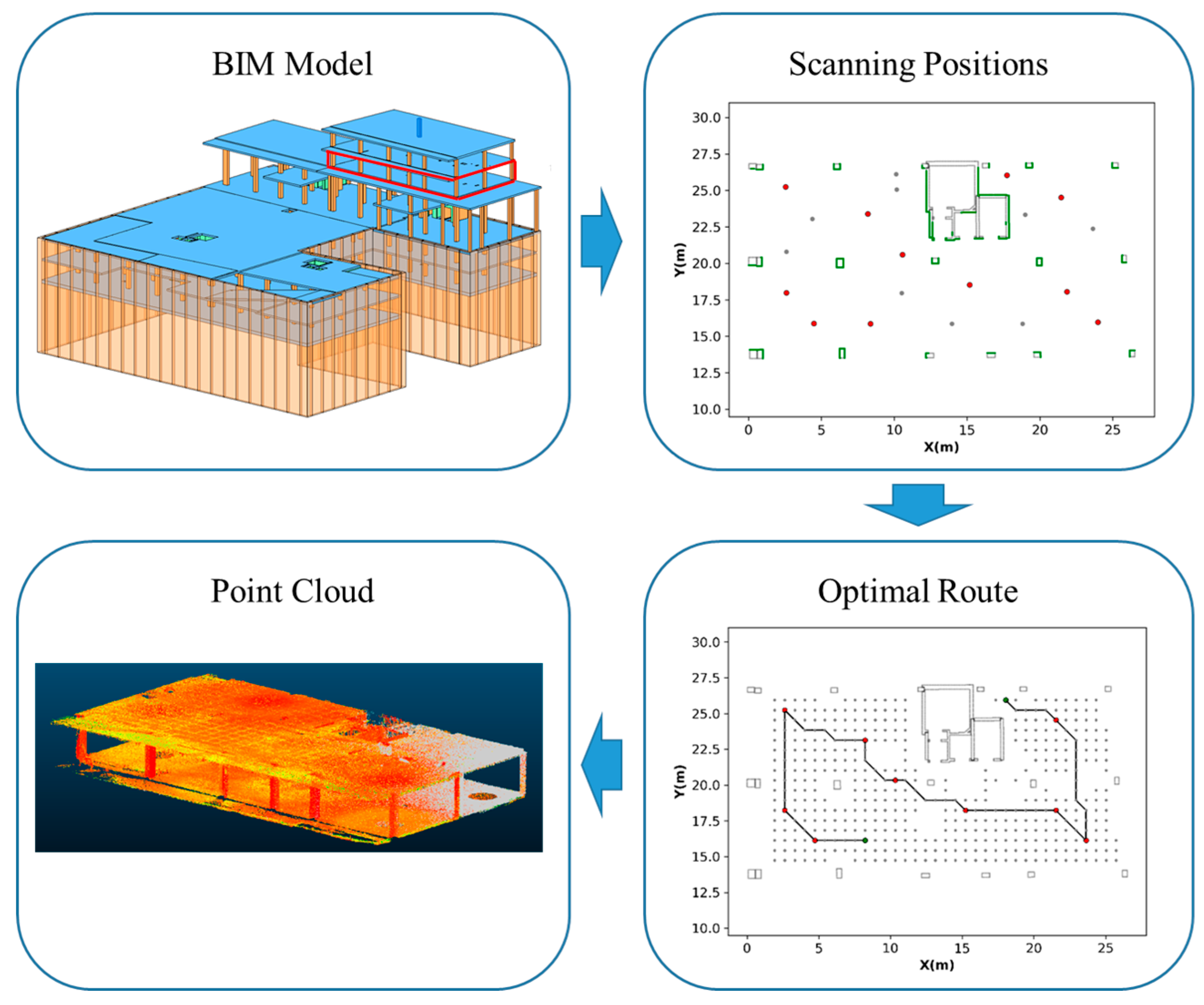
This section presents the results of the entire process from the BIM model to obtaining a point cloud acquired by the acquisition system described in Section 4.1.
The BIM model corresponds to a building under construction during the test in the city of Badalona, Spain. The results shown here comply with one of the floors of the building (highlighted in red in the BIM model shown in Figure 24).
The values of the parameters used to generate the scanning plan are the same as those used in Section 4.2. Figure 23 shows the most relevant results of the process such as the calculated scanning positions and the subsequent optimal route. The calculation of the optimal scan positions took less than 1 second while the optimal route was approximately 2.5 seconds.
Figure 23 also depicts the point cloud obtained by the acquisition system tracking the scan planning calculated by the proposed algorithm. The planning consists of eleven scan positions on a 52.4 metre long route.
5. Conclusions
This paper presents a method to optimize the number and position of scans for Scan-vs-BIM procedures following stop & go scanning method, and the shortest route for an autonomous robot visiting once all the optimal scan positions. The input for the method is a DXF file exported by BIM in which elements are organized by layers. Since semantic information is preserved, scan planning can be directed to certain building elements, or types of elements. This is crucial for control of execution processes. The method implements and compares two strategies for the distribution of scan position candidates: a grid-based method and a triangulation-based method. This aspect is critical, especially in large and complex scenes. Final scan positions are optimized based on visibility and data completeness as stopping criteria, and a probabilistic ant colony optimization algorithm is implemented to obtain a suboptimal route.
The method has been tested in two case studies performing a total of eight simulations. The method has showed to be efficient in terms of time computing. Simulations were carried out for structural elements including beams and columns, and for final elements including walls, doors, etc. In both cases, the grid-based and the triangulation-based distribution have been tested and compared. The results show that the triangulation-based method provides a robust solution in terms of completeness and processing time. In addition, unlike most scan-planning approaches, the path planning problem has been addressed, obtaining reasonable short routes. Scan positions have been correctly distributed on the navigable surface, all of which are accessible by the robotic unit. Scan positions are not too close to each other or to walls.
The method has also been implemented in a complex real case study, providing the robotic unit with the route with the scan positions. From the information provided by the presented algorithm, the robotic unit has performed all the scans autonomously. The point cloud has been generated with a coverage according to the project specifications, high density and precision.
Coverage, candidate positions distribution and selection of optimal locations are crucial aspects for scan planning. These three problems are not independent; coverage is highly dependent on the distribution of candidates, which in turn qualitatively influences the candidate selection process. This interrelation involves reaching a trade-off among the matters already mentioned. Unlike most works focused on scan planning, this paper considers vertical and horizontal structural elements for analysis. Horizontal structural elements, such as beams, are considered to not cause occlusions because the analysis is performed from a 2D perspective.
Future work will involve the study of scan planning from a 3D perspective in a way that not only concerns coverage, but point cloud density and overlapping will be considered as stopping criteria.
Author Contributions
E.F. and L.D.-V. designed the algorithm and performed the experiments, J.B. and H.L provided supervision on the design and implementation of the research and all authors contributed to review and improve the manuscript.
Funding
This research was founded by the Universidade de Vigo, grant nº 00VI 131H 641.02, the Xunta de Galicia, grant no. ED481B 2016/079-0 and the Ministerio de Economia, Industria y Competitividad -Gobierno de España-, grant nº TIN2016-77158, and grant nº RTC-2016-5257-7). This project has received funding from the European Union’s Horizon 2020 research and innovation programme under grant agreement No 769255. This document reflects only the author’s view and the Agency is not responsible for any use that may be made of the information it contains. The statements made herein are solely the responsibility of the authors.
Conflicts of Interest
The authors declare no conflict of interest.
References
- Dai, F.; Rashidi, A.; Brilakis, I.; Vela, P. Comparison of Image-Based and Time-of-Flight-Based Technologies for Three-Dimensional Reconstruction of Infrastructure. J. Constr. Eng. Manag. 2013, 139, 69–79. [Google Scholar] [CrossRef]
- Nikoohemat, S.; Peter, M.; Oude Elberink, S.; Vosselman, G. Exploiting indoor mobile laser scanner trajectories for semantic interpretation of point clouds. ISPRS Ann. Photogramm. Remote Sens. Spat. Inf. Sci. 2017, IV-2/W4, 355–362. [Google Scholar] [CrossRef]
- Son, H.; Kim, C.; Turkan, Y. Scan-to-BIM—An Overview of the Current State of the Art and a Look Ahead. In Proceedings of the International Symposium on Automation and Robotics in Construction, Oulu, Finland, 15–18 June 2015. [Google Scholar]
- Bosché, F. Automated recognition of 3D CAD model objects in laser scans and calculation of as-built dimensions for dimensional compliance control in construction. Adv. Eng. Informatics 2010, 24, 107–118. [Google Scholar] [CrossRef]
- Navon, R. Research in automated measurement of project performance indicators. Autom. Constr. 2007, 16, 176–188. [Google Scholar] [CrossRef]
- Bosche, F.; Haas, C.T. Automated retrieval of 3D CAD model objects in construction range images. Autom. Constr. 2008, 17, 499–512. [Google Scholar] [CrossRef]
- Golparvar-Fard, M.; Bohn, J.; Teizer, J.; Savarese, S.; Peña-Mora, F. Evaluation of image-based modeling and laser scanning accuracy for emerging automated performance monitoring techniques. Autom. Constr. 2011, 20, 1143–1155. [Google Scholar] [CrossRef]
- Bensalah, M.; Elouadi, A.; Mharzi, H. Integrating BIM in railway projects: review & perspectives for morocco & mena. Int. J. Recent Sci. Res. 2018, 9, 23398–23403. [Google Scholar]
- Chen, L.; Luo, H. A BIM-based construction quality management model and its applications. Autom. Constr. 2014, 46, 64–73. [Google Scholar] [CrossRef]
- Latiffi, A.A.; Mohd, S.; Brahim, J. Application of Building Information Modeling (BIM) in the Malaysian Construction Industry: A Story of the First Government Project. Appl. Mech. Mater. 2015, 773–774, 943–948. [Google Scholar] [CrossRef]
- Wang, Q.; Sohn, H.; Cheng, J.C.P. Automatic As-Built BIM Creation of Precast Concrete Bridge Deck Panels Using Laser Scan Data. J. Comput. Civ. Eng. 2018, 32, 04018011. [Google Scholar] [CrossRef]
- Wang, Q.; Guo, J.; Kim, M.-K.; Wang, Q.; Guo, J.; Kim, M.-K. An Application Oriented Scan-to-BIM Framework. Remote Sens. 2019, 11, 365. [Google Scholar] [CrossRef]
- Bosché, F.; Guillemet, A.; Turkan, Y.; Haas, C.T.; Haas, R. Tracking the Built Status of MEP Works: Assessing the Value of a Scan-vs-BIM System. J. Comput. Civ. Eng. 2014, 28, 05014004. [Google Scholar] [CrossRef] [Green Version]
- Pito, R. A solution to the next best view problem for automated surface acquisition. IEEE Trans. Pattern Anal. Mach. Intell. 1999, 21, 1016–1030. [Google Scholar] [CrossRef]
- Krainin, M.; Curless, B.; Fox, D. Autonomous generation of complete 3D object models using next best view manipulation planning. In Proceedings of the 2011 IEEE International Conference on Robotics and Automation, Shanghai, China, 9–13 May 2011; pp. 5031–5037. [Google Scholar]
- Soudarissanane, S.; Lindenbergh, R. Optimizing terrestrial laser scanning measurement set-up. ISPRS - Int. Arch. Photogramm. Remote Sens. Spat. Inf. Sci. 2012, XXXVIII-5/W12, 127–132. [Google Scholar] [CrossRef]
- Scott, W.R.; Roth, G.; Rivest, J.-F. View planning for automated three-dimensional object reconstruction and inspection. ACM Comput. Surv. 2003, 35, 64–96. [Google Scholar] [CrossRef]
- González-Banos, H. A randomized art-gallery algorithm for sensor placement. In Proceedings of the seventeenth annual symposium on Computational geometry-SCG’01, Medford, MA, USA, 3–5 June 2001; ACM Press: New York, NY, USA, 2001; pp. 232–240. [Google Scholar] [Green Version]
- Blaer, P.S.; Allen, P.K. View planning for automated site modeling. In Proceedings of the 2006 IEEE International Conference on Robotics and Automation, Orlando, FL, USA, 15–19 May 2006; pp. 2621–2626. [Google Scholar]
- Jia, F.; Lichti, D.D. AN EFFICIENT, HIERARCHICAL VIEWPOINT PLANNING STRATEGY FOR TERRESTRIAL LASER SCANNER NETWORKS. ISPRS Ann. Photogramm. Remote Sens. Spat. Inf. Sci. 2018, IV-2, 137–144. [Google Scholar] [CrossRef] [Green Version]
- Biswas, H.K.; Bosché, D.F.; Sun, P.M. Planning for Scanning Using Building Information Models: A Novel Approach with Occlusion Handling. In Proceedings of the 32nd International Symposium on Automation and Robotics in Construction and Mining (ISARC 2015), Oulu, Finland, 15–18 June 2015. [Google Scholar]
- ELzaiady, M.E.; Elnagar, A. Next-best-view planning for environment exploration and 3D model construction. In Proceedings of the 2017 International Conference on Infocom Technologies and Unmanned Systems (Trends and Future Directions) (ICTUS), Dubai, United Arab Emirates, 18–20 December 2017; pp. 745–750. [Google Scholar]
- Zhang, C.; Kalasapudi, V.S.; Tang, P. Rapid data quality oriented laser scan planning for dynamic construction environments. Adv. Eng. Informatics 2016, 30, 218–232. [Google Scholar] [CrossRef] [Green Version]
- Surmann, H.; Nüchter, A.; Hertzberg, J. An autonomous mobile robot with a 3D laser range finder for 3D exploration and digitalization of indoor environments. Rob. Auton. Syst. 2003, 45, 181–198. [Google Scholar] [CrossRef]
- Strand, M.; Dillmann, R. Using an attributed 2D-grid for next-best-view planning on 3D environment data for an autonomous robot. In Proceedings of the 2008 International Conference on Information and Automation, Colombo, Sri Lanka, 12–14 December 2008; pp. 314–319. [Google Scholar]
- Potthast, C.; Sukhatme, G.S. A probabilistic framework for next best view estimation in a cluttered environment. J. Vis. Commun. Image Represent. 2014, 25, 148–164. [Google Scholar] [CrossRef] [Green Version]
- Adán, A.; Quintana, B.; Vázquez, A.; Olivares, A.; Parra, E.; Prieto, S.; Adán, A.; Quintana, B.; Vázquez, A.S.; Olivares, A.; et al. Towards the Automatic Scanning of Indoors with Robots. Sensors 2015, 15, 11551–11574. [Google Scholar] [CrossRef] [PubMed] [Green Version]
- Quintana, B.; Prieto, S.A.; Adán, A.; Vázquez, A.S. Semantic scan planning for indoor structural elements of buildings. Adv. Eng. Informatics 2016, 30, 643–659. [Google Scholar] [CrossRef]
- Prieto, S.A.; Quintana, B.; Adán, A.; Vázquez, A.S. As-is building-structure reconstruction from a probabilistic next best scan approach. Rob. Auton. Syst. 2017, 94, 186–207. [Google Scholar] [CrossRef]
- González-de Santos, L.; Díaz-Vilariño, L.; Balado, J.; Martínez-Sánchez, J.; González-Jorge, H.; Sánchez-Rodríguez, A. Autonomous Point Cloud Acquisition of Unknown Indoor Scenes. ISPRS Int. J. Geo-Information 2018, 7, 250. [Google Scholar] [CrossRef]
- Afyouni, I.; Ray, C.; Claramunt, C. Spatial models for context-aware indoor navigation systems: A survey. J. Spat. Inf. Sci. 2012. [Google Scholar] [CrossRef]
- Zlatanova, S.; Liu, L.; Sithole, G.; Zhao, J.; Mortari, F. Space subdivision for indoor applications. GISt Rep. No. 66 2014. [Google Scholar]
- Tran, H.; Khoshelham, K.; Kealy, A.; Díaz-Vilariño, L. Extracting topological relations between indoor spaces from point clouds. ISPRS Ann. Photogramm. Remote Sens. Spat. Inf. Sci. 2017, IV-2/W4, 401–406. [Google Scholar] [CrossRef]
- Flikweert, P. Automatic Extraction of an IndoorGML Navigation Graph from an Indoor Point Cloud; Delft University of Technology: Delft, The Netherlands, 2019. [Google Scholar]
- Lee, J. A Spatial Access-Oriented Implementation of a 3-D GIS Topological Data Model for Urban Entities. Geoinformatica 2004, 8, 237–264. [Google Scholar] [CrossRef]
- Meijers, M.; Meijers, M.; Zlatanova, S.; Pfeifer, N. 3D geo-information indoors: structuring for evacuation. Proceedings of Next generation 3D city models, Bonn, Germany, 21–22 June 2005. [Google Scholar]
- Balado, J.; Díaz-Vilariño, L.; Arias, P.; Frías, E. Point clouds to direct indoor pedestrian pathfinding. ISPRS - Int. Arch. Photogramm. Remote Sens. Spat. Inf. Sci. 2019, XLII-2/W13, 753–759. [Google Scholar] [CrossRef]
- Van Bemmelen, J.; Quak, W.; Van Hekken, M.; Oosterom, P. Van Vector vs. Raster-based Algorithms for Cross Country Movement Planning. In Proceedings of the Auto Carto 11, Minneapolis, MN, USA, 30 October–1 November 1993; pp. 304–317. [Google Scholar]
- Lum, C.; Rysdyk, R. Time constrained randomized path planning using spatial networks. In Proceedings of the 2008 American Control Conference, St. Louis, MO, USA, 11–13 June 2008; pp. 3725–3732. [Google Scholar]
- Li, X.; Claramunt, C.; Ray, C. A grid graph-based model for the analysis of 2D indoor spaces. Comput. Environ. Urban Syst. 2010, 34, 532–540. [Google Scholar] [CrossRef]
- Yuan, W.; Schneider, M. Supporting Continuous Range Queries in Indoor Space. In Proceedings of the 2010 Eleventh International Conference on Mobile Data Management, Kansas City, MI, USA, 23–26 May 2010; pp. 209–214. [Google Scholar]
- Joo, K.; Lee, T.-K.; Baek, S.; Oh, S.-Y. Generating topological map from occupancy grid-map using virtual door detection. In Proceedings of the IEEE Congress on Evolutionary Computation, Barcelona, Spain, 18–23 July 2010; pp. 1–6. [Google Scholar]
- Elseberg, J.; Borrmann, D.; Nüchter, A. One billion points in the cloud—An octree for efficient processing of 3D laser scans. ISPRS J. Photogramm. Remote Sens. 2013, 76, 76–88. [Google Scholar] [CrossRef]
- Fichtner, F.W.; Diakité, A.A.; Zlatanova, S.; Voûte, R. Semantic enrichment of octree structured point clouds for multi-story 3D pathfinding. Trans. GIS 2018, 22, 233–248. [Google Scholar] [CrossRef]
- Aurenhammer, F. Voronoi diagrams—A survey of a fundamental geometric data structure. ACM Comput. Surv. 1991, 23, 345–405. [Google Scholar] [CrossRef]
- Wallgrün, J.O.; Oliver, J. Autonomous Construction of Hierarchical Voronoi-Based Route Graph Representations. In Proceedings of the 4th international conference on Spatial Cognition: Reasoning, Action, Interaction; Springer: Berlin/Heidelberg, Germany, 2005; pp. 413–417, ISBN 3-540-25048-4, 978-3-540-25048-7. [Google Scholar]
- Boguslawski, P.; Mahdjoubi, L.; Zverovich, V.; Fadli, F. Two-graph building interior representation for emergency response applications. ISPRS Ann. Photogramm. Remote Sens. Spat. Inf. Sci. 2016, III-2, 9–14. [Google Scholar] [CrossRef]
- Lamarche, F.; Donikian, S. Crowd of Virtual Humans: A New Approach for Real Time Navigation in Complex and Structured Environments. Comput. Graph. Forum 2004, 23, 509–518. [Google Scholar] [CrossRef]
- Krūminaitė, M.; Zlatanova, S. Indoor space subdivision for indoor navigation. In Proceedings of the Sixth ACM SIGSPATIAL International Workshop on Indoor Spatial Awareness-ISA’14, Dallas, TX, USA, 4 November 2014; ACM Press: New York, NY, USA, 2014; pp. 25–31. [Google Scholar]
- Balado, J.; Díaz-Vilariño, L.; Arias, P.; González-Jorge, H. Automatic classification of urban ground elements from mobile laser scanning data. Autom. Constr. 2018, 86, 226–239. [Google Scholar] [CrossRef] [Green Version]
- Díaz-Vilariño, L.; Frías, E.; Balado, J.; González-Jorge, H. Scan planning and route optimization for control of execution of as-designed BIM. ISPRS - Int. Arch. Photogramm. Remote Sens. Spat. Inf. Sci. 2018, XLII-4, 143–148. [Google Scholar]
- Bresenham, J.E. Algorithm for computer control of a digital plotter. IBM Syst. J. 1965, 4, 25–30. [Google Scholar] [CrossRef]
- Fillmore, J.P.; Williamson, S.G. On Backtracking: A Combinatorial Description of the Algorithm. SIAM J. Comput. 1974, 3, 41–55. [Google Scholar] [CrossRef]
- Dorigo, M.; Gambardella, L.M. Ant colony system: A cooperative learning approach to the traveling salesman problem. IEEE Trans. Evol. Comput. 1997, 1, 53–66. [Google Scholar] [CrossRef]
- Balado, J.; Díaz-Vilariño, L.; Arias, P.; Lorenzo, H. Point clouds for direct pedestrian pathfinding in urban environments. ISPRS J. Photogramm. Remote Sens. 2019, 148, 184–196. [Google Scholar] [CrossRef]
- Dijkstra, E.W. A note on two problems in connexion with graphs. Numer. Math. 1959, 1, 269–271. [Google Scholar] [CrossRef] [Green Version]
- Khoshelham, K.; Díaz Vilariño, L.; Peter, M.; Kang, Z.; Acharya, D. The isprs benchmark on indoor modelling. ISPRS - Int. Arch. Photogramm. Remote Sens. Spat. Inf. Sci. 2017, XLII-2/W7, 367–372. [Google Scholar] [CrossRef]
- Soudarissanane, S.; Lindenbergh, R.; Menenti, M.; Teunissen, P. Scanning geometry: Influencing factor on the quality of terrestrial laser scanning points. ISPRS J. Photogramm. Remote Sens. 2011, 66, 389–399. [Google Scholar] [CrossRef]
Figure 1.
General workflow of the method.

Figure 2.
(a) Building elements considered in this work, (b) elements after discretization in equidistant points.
Figure 2.
(a) Building elements considered in this work, (b) elements after discretization in equidistant points.

Figure 3.
Geometric representation of navigable space (a) in case of the existence of holes and columns (blue lines), (b) in case of the existence of rooms.
Figure 3.
Geometric representation of navigable space (a) in case of the existence of holes and columns (blue lines), (b) in case of the existence of rooms.

Figure 4.
Schema of discretization process when using a grid-based structure (a) in case of the existence of one floor space including a hole and three columns (blue lines) (b) in case of the existence of rooms. Final candidate positions are in green, while discarded candidate positions are in red. Local coordinate systems are represented.

Figure 5.
Workflow of the triangulation process.

Figure 6.
Generation of seed points Se (in blue) for triangulation process for: (a) column, (b) polygon with side < dmin and (c) polygon with side < dmin.
Figure 6.
Generation of seed points Se (in blue) for triangulation process for: (a) column, (b) polygon with side < dmin and (c) polygon with side < dmin.

Figure 7.
Navigable space is partitioned by applying Delaunay triangulation process. (a) Since the polygon that contains navigable space may be concave, some positions obtained after the division can fall out of navigable space (orange). Small triangles are discarded according the parameters lmin and αmin (yellow). (b) A filtering process is conducted to retrieve positions are inside navigable space (points generated by Voronoi process are included). Subsequently, points near obstacles are discarded (red) according to the defined security distance.

Figure 8.
Bresenham algorithm is used to determinate the map cells that are crossed by simulated beam (gray) in visibility analysis. (a) target cell (red) is wrongly classified as visible since it is not occluded by other cells representing building elements, (b) target point (green) is correctly classified as occluded in the ray-casting process.

Figure 9.
Scan optimization process is carried out from candidate positions (green points) to obtain scanning positions (red points). In each iteration the candidate position is selected which maximizes the theoretically acquirable surface (red lines). The black lines represent the surface theoretically acquired from the previously selected positions.

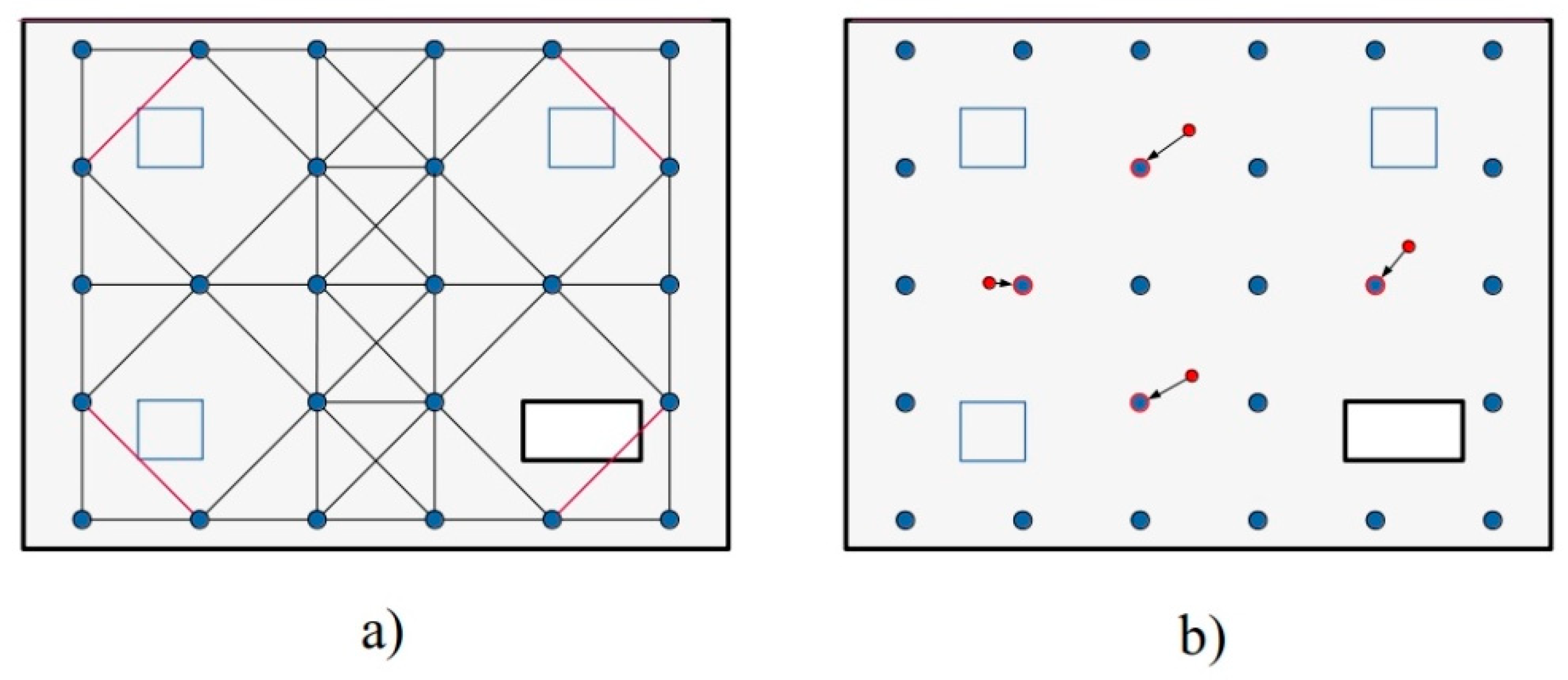
Figure 10.
(a) Graph nodes are 8-connected by edges and the ones intersecting with any no-navigable space are removed (magenta). (b) Scanning positions (red points) are relocated to nearest nodes to them (blue points with red contour).
Figure 10.
(a) Graph nodes are 8-connected by edges and the ones intersecting with any no-navigable space are removed (magenta). (b) Scanning positions (red points) are relocated to nearest nodes to them (blue points with red contour).

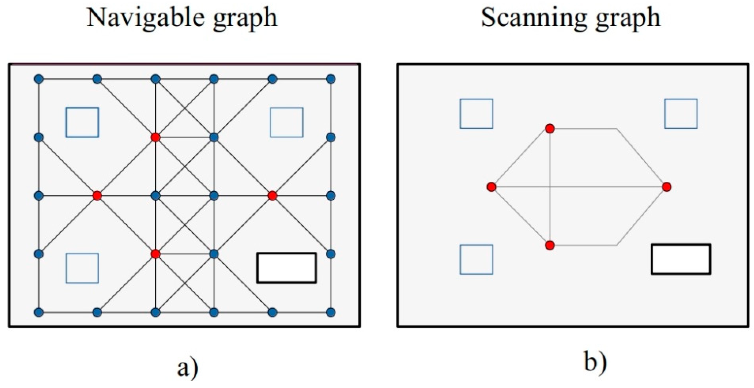
Figure 11.
(a) A navigable graph composed by navigable (blue) and scanning (red) nodes is generated. Then, navigable nodes are abstracted from graph and (b) a simpler one is represented only with scanning nodes (red).
Figure 11.
(a) A navigable graph composed by navigable (blue) and scanning (red) nodes is generated. Then, navigable nodes are abstracted from graph and (b) a simpler one is represented only with scanning nodes (red).

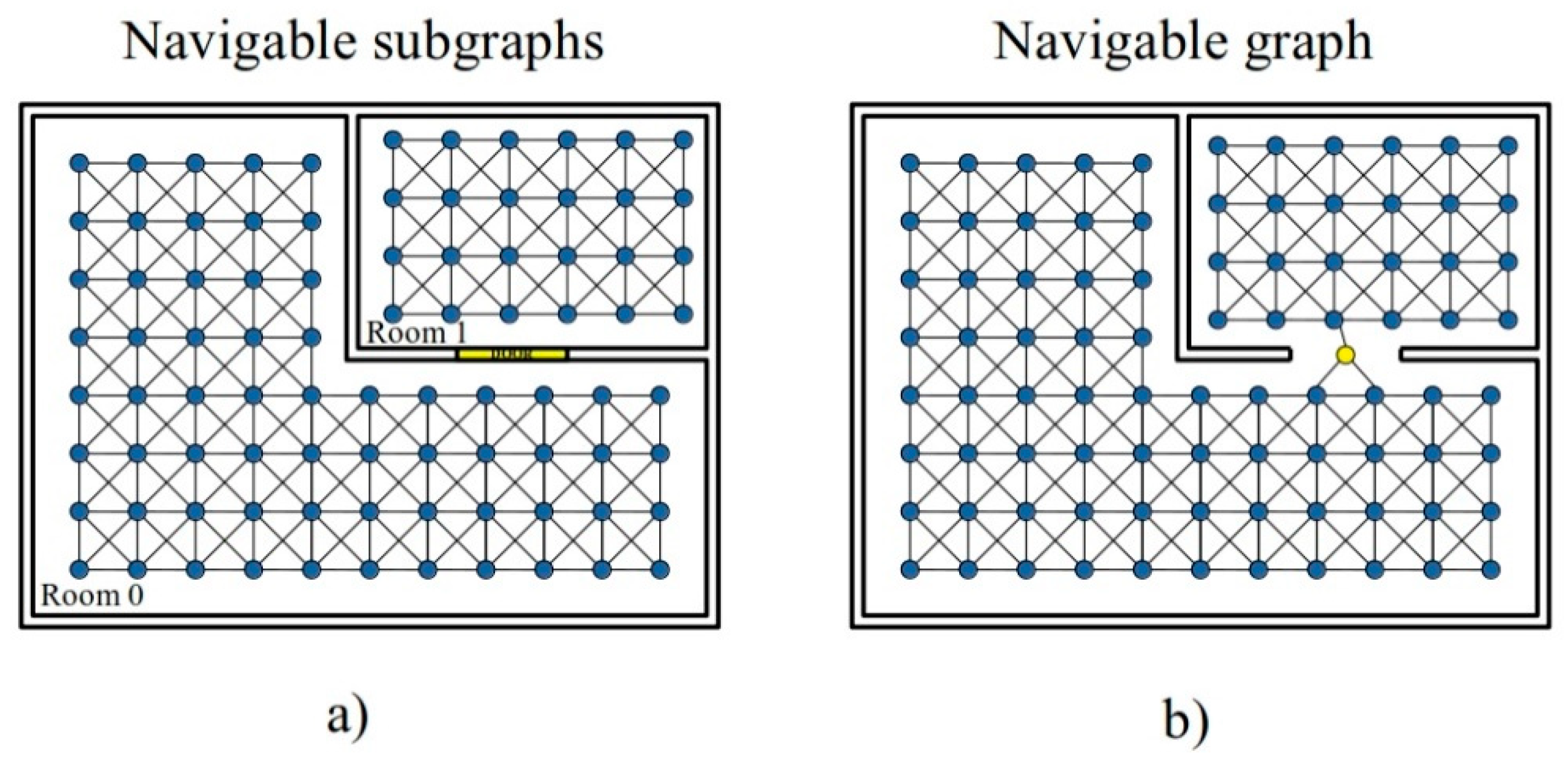
Figure 12.
(a) A subgraph is generated separately for each room. (b) The global graph consists of all subgraphs joined by new nodes corresponding to door positions (yellow).
Figure 12.
(a) A subgraph is generated separately for each room. (b) The global graph consists of all subgraphs joined by new nodes corresponding to door positions (yellow).

Figure 13.
(a) Input BIM model. (b) DXF model of case study 1 and (b) DXF model of case study 2.

Figure 14.
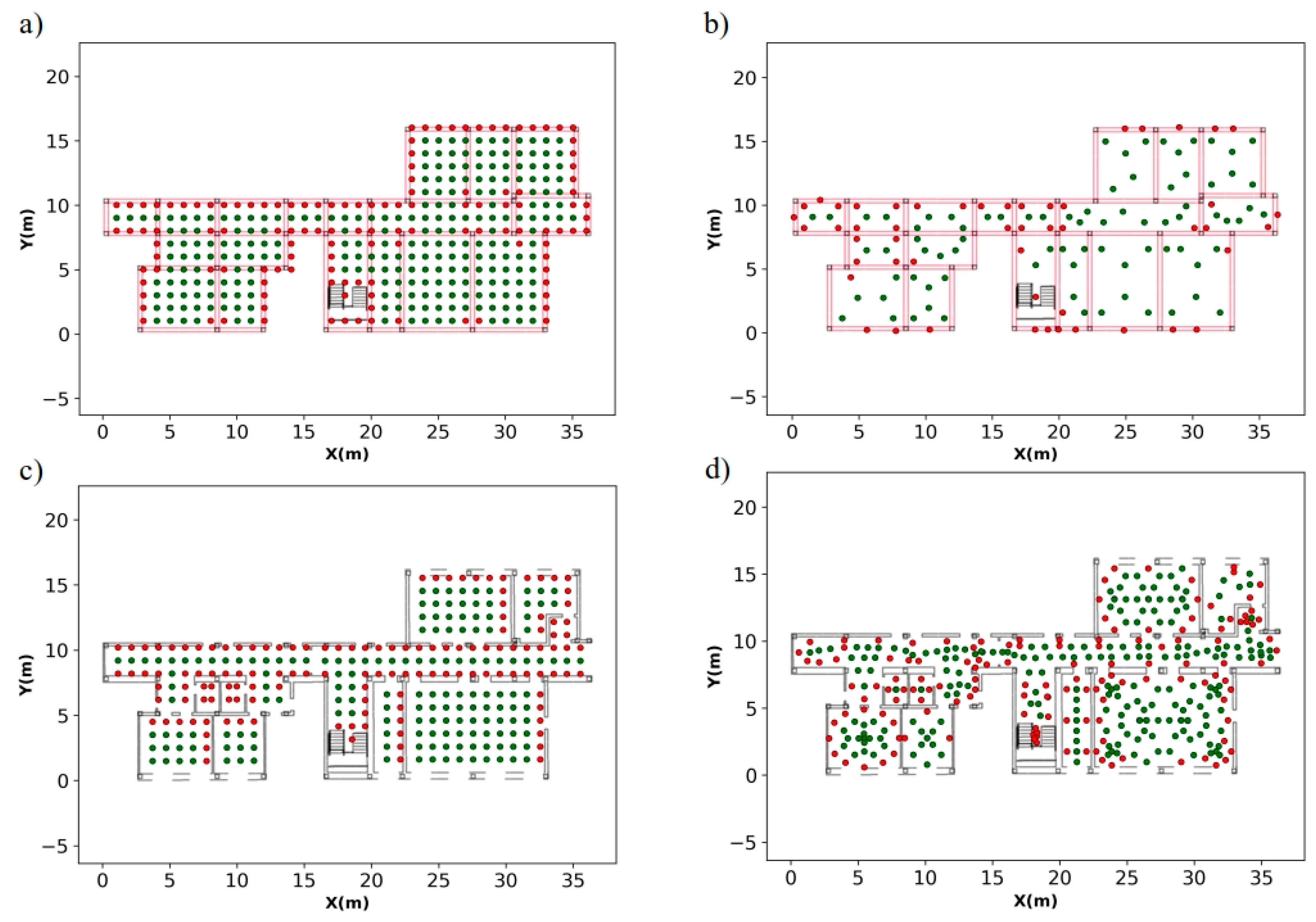
Candidate positions generated by both discretization methods in case study 1: (a) grid-based method in structural phase, (b) triangulation-based method in structural phase, (c) grid-based method with rooms and (d) triangulation-based method with rooms. Horizontal and vertical elements are displayed in magenta and black respectively. Green points represent position reachable by robotic system, unreachable positions are depicted in red.
Figure 14.
Candidate positions generated by both discretization methods in case study 1: (a) grid-based method in structural phase, (b) triangulation-based method in structural phase, (c) grid-based method with rooms and (d) triangulation-based method with rooms. Horizontal and vertical elements are displayed in magenta and black respectively. Green points represent position reachable by robotic system, unreachable positions are depicted in red.

Figure 15.
Candidate positions generated by both discretization methods in case study 2.

Figure 16.
Visibility analysis results obtained from candidates generated in case study 1: (a) grid-based candidate distribution in structural phase, (b) triangulation-based candidate distribution in structural phase, (c) grid-based candidate distribution with rooms and (d) triangulation-based candidate distribution with rooms. Elements determined as visible for analysis process are depicted in green, black points represent no visible elements.

Figure 17.
Visibility analysis results obtained from candidates generated in case study 2.

Figure 18.
Visibility analysis of case study 1 original (a) and rotated (b). Visible elements are coloured in green, while black zones correspond to areas of element to be acquired are not visible from any candidate position.
Figure 18.
Visibility analysis of case study 1 original (a) and rotated (b). Visible elements are coloured in green, while black zones correspond to areas of element to be acquired are not visible from any candidate position.

Figure 19.
Optimization scan position result in case study 1: (a) grid-based method, (b) triangulation-based method, (c) grid-based with scan positions in doors and (d) triangulation-based method with scan positions in doors. Color code: scan positions (red points), candidates scan positions (gray points), acquired elements (green), non-acquired elements (black).

Figure 20.
Optimization scan position result in case study 2.

Figure 21.
Optimal route calculated in case study 1 whose scanning positions were obtained by: (a) grid-based method in structural phase, (b) triangulation-based method in structural phase, (c) grid-based method with rooms and (d) triangulation-based method with rooms. Horizontal and vertical elements are displayed in magenta and black respectively. Green points represent start and end scanning position, the remaining ones are depicted in red.

Figure 22.
Optimal route calculated in case study 2.

Figure 23.
Optimal route calculated in case study 1 with scan positions at doorways in (a) and without scan position at doorways in (b). Color code: scan positions (red points), graph nodes (gray points), start-end positions (green points), scanning-door positions (orange).
Figure 23.
Optimal route calculated in case study 1 with scan positions at doorways in (a) and without scan position at doorways in (b). Color code: scan positions (red points), graph nodes (gray points), start-end positions (green points), scanning-door positions (orange).

Figure 24.
Workflow of the entire process from Building Information Model (BIM) to the acquired point cloud tracking scanning plan generated by the proposed algorithm.
Figure 24.
Workflow of the entire process from Building Information Model (BIM) to the acquired point cloud tracking scanning plan generated by the proposed algorithm.


Table 1.
Input parameters.
| Type of Parameter | Parameter | Abbreviation | Value |
|---|---|---|---|
| Discretization resolution | ddis | 50 mm | |
| Laser range | r | 5 m | |
| Field of view | v | 360º | |
| General | Security Distance | dsec | 0.7 m |
| Coverage | cmin | 90% | |
| Specifics | Resolution grid | rgrid | 1.0 m |
| Door accessibility | door_access | 0.7 m | |
| Doors as scanning position | door_scan | True/False |
Table 2.
Number of units of discretization.
| Scenario | BEAMS | COLUMNS | STAIRS | WALLS | TOTAL |
|---|---|---|---|---|---|
| Case 1 (Structural) | 9066 | 1038 | 891 | - | 10995 |
| Case 1 (Rooms) | - | 1038 | 891 | 6296 | 8225 |
| Case 2 (Structural) | 6044 | 491 | 682 | - | 7217 |
| Case 2 (Rooms) | - | 491 | 682 | 5690 | 6863 |
Table 3.
Results distribution of candidate positions.
| Case of Study | Scenario | Distribution | Number of Candidates | Reachable Candidates | Time (s) |
|---|---|---|---|---|---|
| Case 1 | Structural | Grid-based | 374 | 247 | 0.83 |
| Triangulation-based | 131 | 80 | 0.33 | ||
| Rooms | Grid-based | 297 | 163 | 0.83 | |
| Triangulation-based | 368 | 229 | 1.06 | ||
| Case 2 | Structural | Grid-based | 214 | 182 | 0.80 |
| Triangulation-based | 65 | 35 | 1.10 | ||
| Rooms | Grid-based | 183 | 105 | 0.79 | |
| Triangulation-based | 233 | 138 | 0.68 |
Table 4.
Results of visibility analysis.
| Scenario | Units To Be Acquired | Method | Candidate Positions | Visible Units | Time (s) | Avg. Time (s) |
|---|---|---|---|---|---|---|
| Case 1 (structural) | 10104 | Grid-based | 247 | 9864 | 15.66 | 0.063 |
| Triangulation-based | 80 | 9714 | 4.73 | 0.059 | ||
| Case 2 (structural) | 6535 | Grid-based | 182 | 6230 | 7.73 | 0.042 |
| Triangulation-based | 35 | 6173 | 1.53 | 0.043 | ||
| Case 1 (Rooms) | 7334 | Grid-based | 163 | 3940 | 2.45 | 0.015 |
| Triangulation-based | 229 | 4260 | 3.78 | 0.017 | ||
| Case 2 (Rooms) | 6181 | Grid-based | 105 | 3193 | 1.69 | 0.016 |
| Triangulation-based | 138 | 3417 | 2.18 | 0.016 |
Table 5.
Comparison between different l_rng in structural phase of case study 1.
| l_rng | 5 m | 10 m | |
|---|---|---|---|
| Grid-based | units of visible elements | 9864 units | 9967 units |
| time consumed | 15.66 s | 89.59 s | |
| Triangulation-based | units of visible elements | 9714 units | 9963 units |
| time consumed | 4.73 s | 21.18 s |
Table 6.
Results of optimization process.
| Scenario | Method | Candidate Positions | Scanning Positions | Acquired (%) | Time (s) |
|---|---|---|---|---|---|
| Case 1 (structural) | Grid-based | 247 | 10 | 90.67 | 1.94 |
| Triangulation-based | 80 | 10 | 90.71 | 0.58 | |
| Case 2 (structural) | Grid-based | 182 | 7 | 90.48 | 0.92 |
| Triangulation-based | 35 | 7 | 90.07 | 0.17 | |
| Case 1 (Rooms) | Grid-based | 163 | 17 | 90.36 | 1.36 |
| Triangulation-based | 229 | 19 | 90.71 | 2.19 | |
| Case 2 (Rooms) | Grid-based | 105 | 13 | 92.48 | 0.71 |
| Triangulation-based | 138 | 14 | 90.31 | 0.97 |
Table 7.
Results optimal route calculation.
| Scenario | Method | Scanning Positions | Time Graph Generation (s) | Route Distance (m) | Time Route Calculation (s) |
|---|---|---|---|---|---|
| Case 1 (structural) | Grid-based | 10 | 2.35 | 55.61 | 0.15 |
| Triangulation-based | 10 | 2.38 | 57.02 | 0.15 | |
| Case 2 (structural) | Grid-based | 7 | 1.58 | 42.42 | 0.06 |
| Triangulation-based | 7 | 1.55 | 44.59 | 0.05 | |
| Case 1 (Rooms) | Grid-based | 17 | 3.02 | 103.99 | 0.63 |
| Triangulation-based | 19 | 4.27 | 100.34 | 0.94 | |
| Case 2 (Rooms) | Grid-based | 13 | 1.87 | 88.10 | 0.29 |
| Triangulation-based | 14 | 1.89 | 87.27 | 0.35 |
© 2019 by the authors. Licensee MDPI, Basel, Switzerland. This article is an open access article distributed under the terms and conditions of the Creative Commons Attribution (CC BY) license (http://creativecommons.org/licenses/by/4.0/).
Share and Cite
MDPI and ACS Style
Frías, E.; Díaz-Vilariño, L.; Balado, J.; Lorenzo, H. From BIM to Scan Planning and Optimization for Construction Control. Remote Sens. 2019, 11, 1963. https://0-doi-org.brum.beds.ac.uk/10.3390/rs11171963
AMA Style
Frías E, Díaz-Vilariño L, Balado J, Lorenzo H. From BIM to Scan Planning and Optimization for Construction Control. Remote Sensing. 2019; 11(17):1963. https://0-doi-org.brum.beds.ac.uk/10.3390/rs11171963
Chicago/Turabian StyleFrías, Ernesto, Lucía Díaz-Vilariño, Jesús Balado, and Henrique Lorenzo. 2019. "From BIM to Scan Planning and Optimization for Construction Control" Remote Sensing 11, no. 17: 1963. https://0-doi-org.brum.beds.ac.uk/10.3390/rs11171963
Note that from the first issue of 2016, this journal uses article numbers instead of page numbers. See further details here.