Volumetric Analysis of Reservoirs in Drought-Prone Areas Using Remote Sensing Products


German Remote Sensing Data Center (DFD), German Aerospace Center (DLR), Münchener Straße 20, 82234 Weßling, Germany
*
Author to whom correspondence should be addressed.
Remote Sens. 2019, 11(17), 1974; https://0-doi-org.brum.beds.ac.uk/10.3390/rs11171974
Submission received: 23 July 2019
/
Revised: 10 August 2019
/
Accepted: 19 August 2019
/
Published: 22 August 2019
(This article belongs to the Special Issue Lake Remote Sensing)
Abstract
:Globally, the number of dams increased dramatically during the 20th century. As a result, monitoring water levels and storage volume of dam-reservoirs has become essential in order to understand water resource availability amid changing climate and drought patterns. Recent advancements in remote sensing data show great potential for studies pertaining to long-term monitoring of reservoir water volume variations. In this study, we used freely available remote sensing products to assess volume variations for Lake Mead, Lake Powell and reservoirs in California between 1984 and 2015. Additionally, we provided insights on reservoir water volume fluctuations and hydrological drought patterns in the region. We based our volumetric estimations on the area–elevation hypsometry relationship, by combining water areas from the Global Surface Water (GSW) monthly water history (MWH) product with corresponding water surface median elevation values from three different digital elevation models (DEM) into a regression analysis. Using Lake Mead and Lake Powell as our validation reservoirs, we calculated a volumetric time series for the GSWMWH–DEMmedian elevation combinations that showed a strong linear ‘area (WA) – elevation (WH)’ (R2 > 0.75) hypsometry. Based on ‘WA-WH’ linearity and correlation analysis between the estimated and in situ volumetric time series, the methodology was expanded to reservoirs in California. Our volumetric results detected four distinct periods of water volume declines: 1987–1992, 2000–2004, 2007–2009 and 2012–2015 for Lake Mead, Lake Powell and in 40 reservoirs in California. We also used multiscalar Standardized Precipitation Evapotranspiration Index (SPEI) for San Joaquin drainage in California to assess regional links between the drought indicators and reservoir volume fluctuations. We found highest correlations between reservoir volume variations and the SPEI at medium time scales (12–18–24–36 months). Our work demonstrates the potential of processed, open source remote sensing products for reservoir water volume variations and provides insights on usability of these variations in hydrological drought monitoring. Furthermore, the spatial coverage and long-term temporal availability of our data presents an opportunity to transfer these methods for volumetric analyses on a global scale.
1. Introduction
The global fresh water reservoirs constitute as important sources of fresh water storage, transportation and provision [1]. In addition to the fresh water supply, they are major water providers for the industry, hydropower plants and agriculture sector [2]. They are the regulators for flood control, river runoff and make up important elements of hydrological-biogeochemical processes and green house emissions due to their still-water natural state [2,3]. Dam constructions therefore, have been a crucial feature of the anthropocene, especially in the 20th century when majority of the world’s dams were constructed [4]. According to the International Commission on Large Dams (https://www.icold-cigb.org/) the global number of large dams (>15 m high) increased from 5750 to more than 41,000 between 1950 and 2004 [3]. While China, Brazil, Russia, Canada and the USA are the world’s top five hydroelectricity producers [4], most of the global dam projects and reservoirs are located in North America and Asia [5,6]. With such rapid growth in the number of reservoirs, there is a need for a globally consistent, reliable and openly accessible reservoir water storage information system that could be used to monitor water volume patterns. Existing reservoir water volume data are primarily available for developed countries and are seldom openly accessible [7]. Conventional reservoir water level measuring strategies include using in situ gauging stations which are stationed at the river mouths, bridges or weirs [8]. However, to assess water dynamics on larger spatial scales, reliance on gauging stations is not always practical due to lack of accessibility to the region and geopolitical constraints in the data acquisition [9,10]. In the context of global changes in climate and drought occurrence patterns, water level and storage assessment of reservoirs is a challenging task because water levels and storage in reservoirs can vary considerably depending upon precipitation, river inflow, industrial discharge and outflow quantity from evaporation, groundwater seepage, withdrawal and river outflow [8]. Moreover, the global dispersal and availability of fresh water is highly irregular and often does not correlate with human population distributions or socio-economic requirements [2].
Remote sensing data can provide long-term and cost effective solutions for the reservoir and inland water body monitoring and analysis due to their global coverage and long temporal availability [11]. The U.S. Geological Survey’s (USGS) Landsat program currently has the longest global spatio-temporal coverage [12] and has been effectively used in water surface mapping and area calculations [13,14,15]. For water volume analyses, a combination of Landsat data with bathymetric and topographic information [16,17,18] and more recently, altimetry data from radar satellites such as TOPEX/Poseidon, Envisat, Jason-1, Jason-2, ERS-2 have been effectively used [8,10,19,20,21,22,23,24,25]. Alternatively, numerous studies have used the total water storage (TWS) data derived from temporal gravity field variations captured by Global Recovery and Climate Experiment (GRACE) for fresh water availability and storage analyses [26,27,28,29,30]. In the recent years, processed time series products for water surface areas and elevation have become available which show great potential for water volume analyses. Since 2016, the global surface water (GSW) layers produced by the EU’s Joint Research Center (JRC) offer a pre-processed and validated, Landsat based global water cover time series that spans over three decades (1984–2015) [31]. These time series are available on monthly and yearly scales. Similarly, ‘Database for hydrological time series over inland waters’ (DAHITI); an open source altimetry database that combines surface water elevation information from multiple sensors, is available since 2015 [32]. Surface water elevation and area information extracted from these data were successfully combined by Busker et al. (2019) to derive volume variations in reservoirs based on linear area–elevation hypsometric relationship [33]. Based on variable degrees of area–elevation linearity for 137 lakes around the world, Busker et al. (2019) estimated volume variations for reservoirs between 1984 and 2015 [33].
Studies mentioned here rely primarily on altimetry methods or gravity field variation based GRACE data for surface water elevation-water storage for volumetric analyses. The GRACE was launched in 2002 and acquired data at 1 degree spatial resolution (>100 km) which is insufficient for the analysis of reservoirs of smaller size. With the exception of TOPEX/POSEIDON (1992) and ERS-2 (1995) missions, the temporal coverage of altimeter data and GRACE volumetric information begins only in year 2002. Apart from the currently active Jason-2 and SARAL/AltiKa sensors, the data acquisition for other altimeter missions was concluded by 2013. These discrepancies create significant temporal
gaps in the surface water elevation information time series. In the spatial context, the pulse-limited footprints of radar satellites over inland water bodies can cover up to 16 km [34]. Regions of smaller water bodies contained within these footprints can result in an inaccurate estimate of surface elevation due to varying altimeter wave-forms that potentially represent both water and other land cover types [32,34]. While altimetry data continues to grow, its applicability in global water volume analyses remains limited due to the lack of wall-to-wall coverage and spatio-temporal restrictions.
This study focuses on utilizing the complete temporal range (32 years) of the GSW data in combination with digital elevation models (DEM) to acquire a near-continuous reservoir volume variation time series between 1984 and 2015. The study is designed to achieve the following objectives: First, we assess ‘area–elevation’ hypsometry relationship for the validation reservoirs using the GSW time series product and the corresponding DEM data to establish applicability of DEMs for volume variation estimations. Next, we apply our methodology to reservoirs in California to estimate state-wide reservoir volume variations. Finally, we compare volume variations in reservoirs to multiscalar drought index to assess correlations between water volume declines in reservoirs and drought patterns.
2. Study Area
2.1. Lake Mead and Lake Powell
Drainage areas and storage volumes vary considerably in the continental United States. The dam storage capacities in central-western and southwestern United States are approximately four times higher than the dam mean annual runoff [35]. Created by the construction of the Hoover dam, Lake Mead is the largest reservoir in the US by water storage capacity and the second largest reservoir by surface water area, only surpassed by Lake Powell [36]. Lake Powell, formed by Glen Canyon dam, is the reservoir with the largest surface water area and sits further upstream on the Colorado river. Combined, these two reservoirs have a storage capacity of 64 billion cubic meters (BCM) that accounts for 85% of the Colorado river basin [37]. The Colorado river basin region has experienced extensive drought periods in the past 50–90 years [38]. These conditions are reflected in water levels of both Lake Mead and Lake Powell. Most recently, both lakes have experienced significant drops in water storage due to drought periods between 2000 and 2010 [8,39] (Figure 1a). Barring year 2012, when drought conditions were shortly reversed due to above average inflow of melting snow from the Rocky mountains detected by the NASA’s Earth Observatory (https://earthobservatory.nasa.gov/world-of-change/LakePowell), river inflow into Lake Powell has been below average for 12 out of 15 recorded years between 2000 and 2014 [40]. We used Lake Mead and Lake Powell in our preliminary area–elevation regression analysis.
2.2. Reservoirs in California
California’s water history and historical drought conditions have been well documented [40]. The Pacific ocean provides the state with moisture that is cooled as it moves up the Sierra Nevada and Transverse mountain ranges on the eastern border and condenses in rain and snow precipitation. This precipitation is the main water source for the state’s largest rivers and watersheds [41]. However, California also shows some of the highest coefficients of variation in precipitation for a water year [42]. On a regional scale, state’s south eastern desert and the northern areas can experience a wetter and a more moist weather conditions in the midst of statewide drought [41]. We used 184 reservoirs in California in our analysis. With areas of reservoirs ranging between 0.5 km2–500 km2, more than half of these reservoirs are used for irrigation and water supply. Majority of the reservoirs in the state are located in the central and northern regions inside San Joaquin and Sacramento drainage regions (Figure 1b) which have experienced droughts frequently in the past three decades [40].
3. Materials and Methods
3.1. Global Surface Water
Processed in Google Earth Engine (GEE), the Global Surface Water (GSW) data is based on 3 million images from Landsat 4, 5, 7 and 8 satellites and maps global surface water changes from March 1984 to October 2015 [31]. It offers an accurate and validated estimation of water dynamics on a global scale at 30 m resolution [33,43]. At multi-temporal levels, the GSW evaluates presence or absence of water pixels on monthly (380 layers) and yearly (32 layers) scales. Based on these temporal water profiles, the GSW comprises of the following six mapped data sets: ‘occurrence’, ‘occurrence change intensity’, ‘recurrence’, ‘seasonality’, ‘transitions’ and ‘maximum extent’. These layers can be downloaded through JRC’s online portal (Global Surface Water Data Access: https://global-surface-water.appspot.com/download). The long-term monthly and yearly water time series are available for download through GEE. We used the ‘monthly water history’ (MWH) and the ‘maximum extent’ (ME) GSW layers in our analysis. The MWH was produced from available Landsat scenes for every month starting March 1984 to October 2015. For each scene, the GSW classifies image pixels into ‘water’, ‘not water’ (land surface) and ‘no observation’ (missing data or snow, ice, clouds). Derived from the MWH, the ME layer accounts for every pixel that was ever classified as water in the 32 years of study. When put together, the ME layer combines all the scenes collected over 32 years into one continuous map showing locations where water was detected [31].
3.2. Digital Elevation Models
We downloaded the three DEMs generated by TanDEM-X (TerraSAR-X add-on for digital elevation measurements), the Shuttle Radar Topography Mission (SRTM) and the Advanced Land Observing Satellite (ALOS) to assess median elevation values along reservoir boundaries. Acquired between December 2010 and January 2015, the global DEM from TanDEM-X was produced in September 2016. With absolute horizontal-vertical accuracy below 10 m and relative accuracy below 2 m for slopes <20% and below 4 m for slopes ≥ 20% [44], TanDEM-X DEM offers an extensively detailed, global 3-dimensional map of the Earth’s surface [45]. The SRTM acquired data during 11 days in February 2000 and produced a topographical map of regions between 60 degrees north and south [46]. The final SRTM-DEM product shows 12.6 m and 9 m horizontal and vertical accuracy respectively [47]. The ALOS satellite equipped with PRISM sensor for stereo mapping was launched in January 2006 and operated for five years [48]. The ALOS collected global imagery with less than 30% cloud cover (about 3 million images) to produce a 5 m DEM commercial product. Vertical and horizontal accuracies for this product were expressed as RMSEs and were recorded at 5 m in both directions [49]. By using ‘median’ and ‘average’ resampling techniques on the original 5 m model, a 30 m resolution ‘ALOS DSM: Global 30 m’ open source multi-band DEM was produced. We used open source versions of the three DEM products available at 30 m (SRTM, ALOS) and 90 m (TanDEM-X) spatial resolutions.
3.3. Standardized Precipitation Evapotranspiration Index
We used Standardized Precipitation Evapotraspiration Index (SPEI) [50] to analyze water volume variation-drought dynamics. Published in 2010, SPEI is based on Standardized Precipitation Index (SPI) and uses climate balance equations proposed by Thonthwaite [51] to produce drought index at different monthly time scales [50]. While global SPEI data is produced at 0.5 degree resolution (between 45–50 km), it is available at a finer resolution (4 km) in the continental United States due to well documented precipitation and temperature time series maintained by the US Historical Climatology Network and availability of high-resolution ‘Parameter-elevation Regression on Independent Slopes Model’ (PRISM: https://climatedataguide.ucar.edu/climate-data/prism-high-resolution-spatial-climate-data-united-states-maxmin-temp-dewpoint) for the US. Produced by Abatzoglou et al., we accessed these data on The West Wide Drought Tracker (WWDT: https://wrcc.dri.edu/wwdt/time/) [52] to download monthly time series for the SPEI at 3, 6, 9, 12, 18, 24, 36, 48 and 60 month intervals at San Joaquin drainage level.
3.4. Validation and Auxiliary Data
We validated volume variation estimations for Lake Mead and Lake Powell using the United States Geological Survey’s (USGS) in situ data that is available for download from the National Water Information System (NWIS: https://waterdata.usgs.gov/nwis/current) and the United States Bureau or Reclamation (USBR: https://www.usbr.gov/rsvrWater/HistoricalApp.html). The NWIS offers reservoir storage data for Lake Mead recorded at Hoover dam as a daily time series. Similarly, the USBR offers Lake Powell storage time series on daily and monthly scale. We downloaded San Joaquin drainage boundaries via National Oceanic and Atmospheric Administration’s Physical Sciences Division (https://www.esrl.noaa.gov/psd/data/usclimdivs/boundaries.html) portal. Reservoir boundaries and meta data for Lake Powell, Lake Mead and Californian reservoirs were acquired from ‘Global Reservoir and Dam’ database (GRanD) available through NASA’s ’Socioeconomic Data and Applications Center’ (SEDAC: http://sedac.ciesin.columbia.edu/data/set/grand-v1-reservoirs-rev01) portal.
3.5. Estimating Water Volume Variations
In this study we adapted and modified the methodology established by Busker et al. (2019) [33]. While keeping the GSW-MWH as input for monthly surface water area calculations, we replaced altimetry input with time series of elevation data derived from interception of the monthly GSW-MWH water mask boundaries with different DEMs. Our methodology involved the following procedures (Figure 2):
- Acquiring JRC-Global Surface Water MWH and ME layers to calculate monthly surface water area (WA) time series and derive monthly water extent boundaries between 1984 and 2015.
- Extracting median DEM values (WH) from SRTM, ALOS and TanDEM-X raster layers at reservoir monthly water extent boundaries for every month between 1984 and 2015.
- Running regression analysis on WA-WH pairs to check for linearity between the GSW surface water areas and each of the three DEMs.
- Using water area-DEM combinations with linear hypsometry to generate volume variation time series between 1984 and 2015.
- Correlating volume variations with SPEI for San Joaquin drainage at different monthly time scales.
The reservoir water volume can be approximated using reservoir hypsometry. We assessed the reservoir water area–elevation relationship by running a regression analysis on the pairs of monthly water areas and median DEMs values at monthly water extent boundaries. We used slope and intercept coefficients to estimate water volume variations for the available time series of reservoirs. Figure 3 shows a functional linear relationship between median DEM elevation (WH) and water extent areas (WA) which is given by the equation:
where ‘b’ and ‘a’ are intercept and slope derived from linear regression respectively. The volumetric variations in water bodies can be estimated using surface water area and surface water elevation if the two variables follow this linear hypsometric relationship [33]. With this relationship, Busker et al. (2019) estimated water volume using the following equation:
where WH is the surface water level, WA is the surface water area and ‘b’ is the elevation intercept. Busker et al. (2019) modified this equation further, to acquire water volumetric time series using only WH or WA:
where and are the volumes estimated using water area or water level [33].
We used the ME layer for a precise delineation of monthly water masks of reservoirs from the MWH time series between 1984 and 2015. Using the ME boundary as a reference for the maximum water extent for the reservoirs, we calculated relative proportions of ‘water’ pixels for each of the MWH layer. For Lake Mead and Lake Powell, we removed months showing more than 1% ‘no observation’ pixels for an accurate estimate of water area calculation. Based on the three DEM products, we extracted median DEM value for the lake boundary individually for each month from the MWH layers. As the TanDEM-X elevation values are represented in ‘Ellipsoidal’ heights and the SRTM and the ALOS models are represented in ‘Orthometric’ heights, we converted and resampled the TanDEM-X height values to Orthometric format to standardize elevation values across three DEMs used. Using linear regression, we computed R2 values for all the valid monthly pairs of surface water area and median DEM elevation. We calculated volume estimates for all the three DEM products using slope and intercept parameters generated from linear relationship between respective water extent areas and median DEM values. Using Equations (3) and (4) we computed two volume series (elevation-VH and area-VA derived) for each DEM. To calculate volume variation, we chose the volume estimations for the first recorded year as the reference year and subtracted volumes from each of the subsequent years. Depending upon the water levels found in subsequent years, these variations could be either positive or negative. We included corresponding months for in situ storage capacity data in this process to compare the performances of individual DEMs with ground station water storage estimates.
We set a marginally higher, 5% ‘no observation’ pixel threshold for filtering GSW-MWH data for Californian reservoirs to calculate water volume variations. This allowed for a better balance between availability of valid data and volume variation precision [33]. Due to variable data availability in the Landsat archive, we considered the first year of valid data acquisition for each reservoir in the state as the individual reference year. For volume variation estimates, we chose TanDEM-X sensor for California as it demonstrates superior overall horizontal and vertical accuracy [45,53] compared to ALOS and SRTM models. We combined the TanDEM-X DEM with ‘VA’ volumetric equation due to its higher correlation with in situ storage volume time series for validation reservoirs. Based on linear WA-WH relationships, we calculated volume variations for reservoirs in California.
3.6. Water Volume Variation and SPEI
We chose San Joaquin drainage climatic division in California to assess relationship between water volume declines and variations in the SPEI. San Joaquin drainage region has experienced frequent droughts between years 1984 and 2015 with some counties in the region proclaiming droughts during multiple years of dry periods [41]. Using Pearson’s correlation we compared water volume variations in the San Joaquin drainage reservoirs with the SPEI at multiple monthly scales to assess patterns of volume declines in reservoirs and changing SPEI values during the same time period.
4. Results
4.1. Hypsometry Relationship between GSWarea-DEMmedian
The regression analysis on validation reservoir data showed a linear WA-WH hypsometry relationship for the ALOS and TanDEM-X DEMs (Figure 4). Regression with in situ records showed highest linearity. Both ALOS (R2 = 0.764) and TanDEM-X (R2 = 0.799) elevation models showed high linear relationship with water area extent for Lake Mead. For Lake Powell, ALOS estimated a stronger linear trend with water areas (R2 = 0.900) compared to TanDEM-X (R2 = 0.812). The SRTM median DEM values showed the lowest linear hypsometry with water areas with R2 = 0.061 for Lake Mead and R2 = 0.555 for Lake Powell. We did not include the SRTM data further in our analysis.
4.2. Volumetric Time Series Results for DEM-VA-VH Combinations in Validation Data
After applying the 1% ‘no observation’ pixel threshold to the MWH data, we used 132 and 130 monthly records for Lake Mead and Lake Powell as validation reservoirs. Figure 5 and Figure 6 show variations in water volumes for Lake Mead and Lake Powell between years 1984 and 2015. Both lakes are part of the Colorado river basin and therefore volume variations in both lakes mirrored one another. Compared to Lake Powell, the volumetric time series (VH and VA) derived from the ALOS and TanDEM-X showed lower deviations from in situ water volume time series for Lake Mead (Figure 5). Figure 5 and Figure 6 also show the minimal to completely absent water variation curves for the SRTM DEM due to its non-linear relationship with the GSW-MWH water areas. Both lakes have a maximum storage capacity of approximately 30 km3 [54,55] which was maintained during years 1984–1988 and again between 1995 and 2000. Our analysis detected the volume decline between years 1987 and 1992 due to an extended drought period [40] accurately. Between 1987 and 1992 Lake Mead and Lake Powell lost more than 5 km3 and 10 km3 of water volume respectively (Figure 5 and Figure 6). Lakes recovered their lost volumes between 1993 and 1998 and regained full capacities between 1998 and 2000. Prolonged drought conditions following year 2000 caused a significant water volume loss in both lakes. Water volume of Lake Mead decreased by 10 km3 between 2000 and 2005 and by another 5 km3 between 2005 and 2015. By the end of the study period, Lake Mead had lost approximately 16 km3 of water compared to its volume in 2000 (Figure 5). Lake Powell experienced the largest decline in volume between years 2000 and 2004. By mid-2004, the lake had lost more than 17 km3 of water compared to the volume in 2000. The lake recovered considerably between 2005 and 2012 regaining 5–7 km3 of water before losing the retained volume after 2012. Overall, Lake Powell lost 15 km3 of water between 1984 and 2015 (Figure 6).
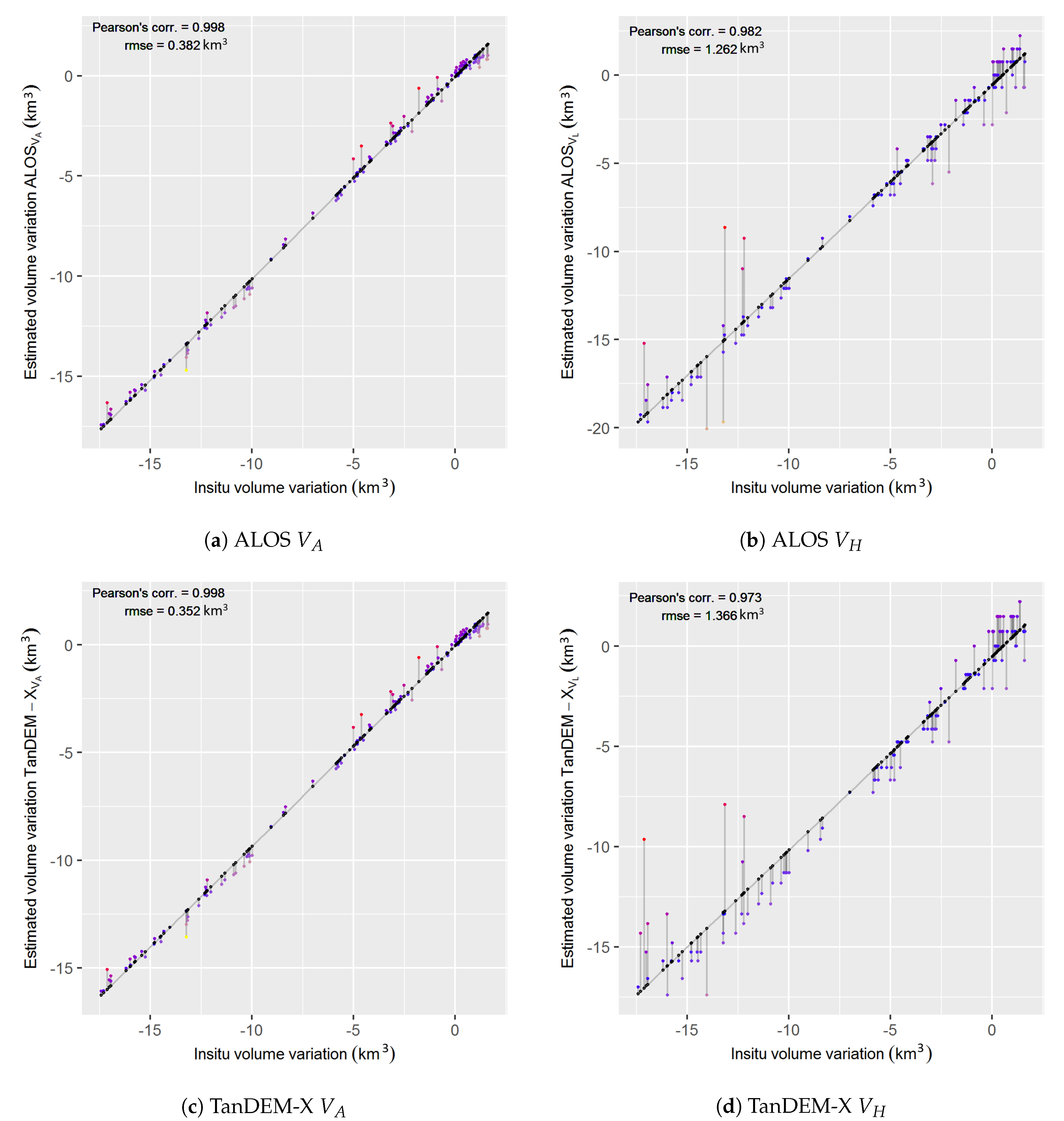
4.3. Accuracy of Volume Variation Estimations
We assessed accuracy of remotely sensed water volume variations by comparing all combinations of volumetric time series (VH and VA) and the ALOS, TanDEM-X DEMs with in situ volume variations for Lake Mead and Lake Powell. We used Pearson’s correlation and root mean square error (RMSE) to evaluate deviation of estimated volume variations from the in situ water storage variations. All remotely sensed volume variations showed high correlations with the in situ data (Figure 7 and Figure 8). The area derived (VA) volumetric time series for ALOS and TanDEM-X DEMs showed higher linearity with the in situ storage time series (RMSE < 1 km3) (Figure 7a,c and Figure 8a,c). The elevation derived (VH) volume variations showed higher deviations (RMSE > 1 km3) from in situ data in comparison to area derived variation results (Figure 7b,d and Figure 8b,d).
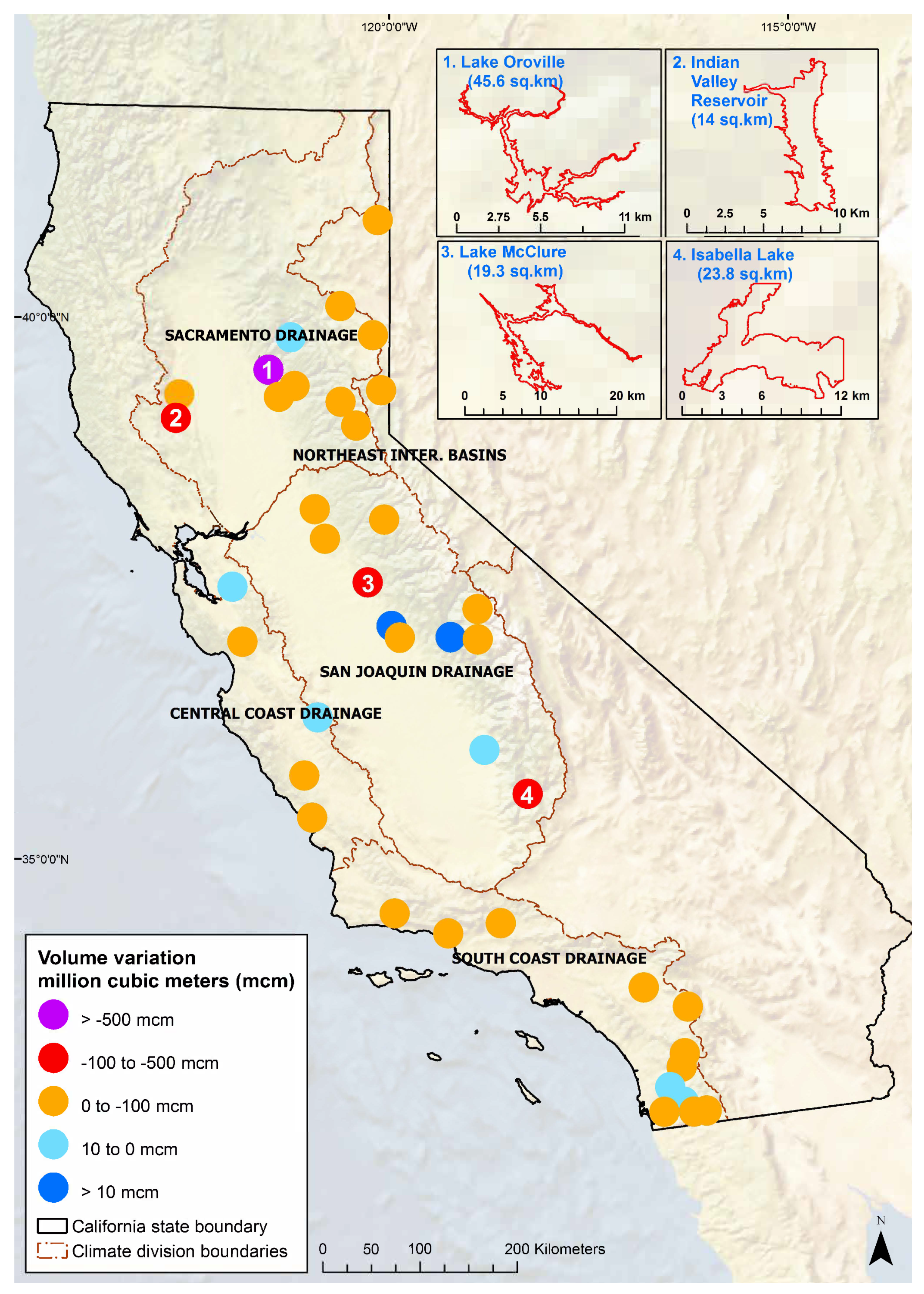
4.4. Volume Variations for Reservoirs in California
The regression analysis for the 184 reservoirs in California showed variable linearity. We only considered reservoirs with a linear ‘area–elevation’ hypsometry and calculated volume variations for the top 40 reservoirs with the strongest linear hypsometry (R2 > 0.75) between median TanDEM-X values and GSW surface water areas. Figure 9 shows the median volume variation in million cubic meters (mcm) across the study period for each reservoir. Depicted by circles, different colors indicate different thresholds of variation with net gain or loss of water volume. We recorded a ‘net water loss’ in 32 reservoirs between 1984–2015 with majority of the reservoirs losing up to 100 mcm water during this period. Median volume variation and loss were higher (>100 mcm) in San Joaquin and Sacramento drainage regions in reservoirs such as Lake Oroville (−653 mcm), Lake McClure (−216 mcm), Isabella Lake (−131 mcm) and Indian Valley Reservoir (−103 mcm). Eight reservoirs showed a ‘net water gain’ during the study period. H.V Eastman Lake and Hensley Lake in San Joaquin drainage recorded the largest net water volume gains (>10 mcm) during the study period. Irrespective of net volume gain-loss, we detected significant water volume declines during four distinct periods (1986–1992, 2000–2005, 2007–2009 and 2012–2015) (Figure 10) in the state. Volume losses were marginally lower during the 2000–2005 and 2007–2009 periods compared the 1987–1992 and 2012–2015. Reservoirs recovered their lost water volume between years 1992 and 2000 and again between years 2009 and 2012. However, volume declines in the subsequent years resulted in a net loss of water storage for the majority of the reservoirs in the state.
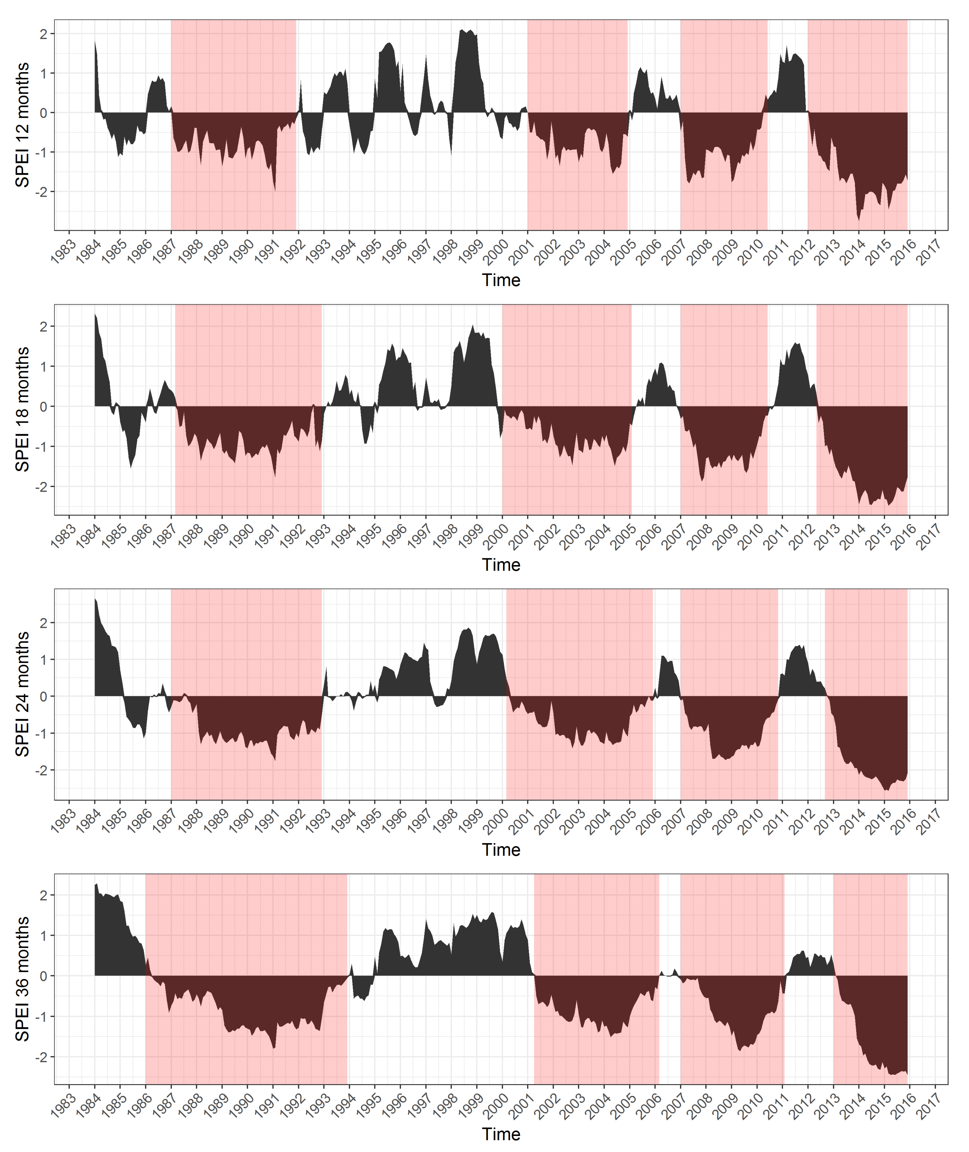
4.5. Reservoir Water Volume Variations and SPEI
The drought periods in California (1987–1992, 2007–2009 and 2014 onward) [41] were accurately identified in our analysis through significant volume declines detected during these years. Additionally, we detected a prolonged dry period between years 2000 and 2003 (Figure 10). For a more detailed assessment relating reservoir water dynamics and drought patterns, we compared water volume variations with SPEI time series in the San Joaquin drainage. At the scales of 12–18–24–36 months, the negative index values indicated the drought years for the San Joaquin drainage (Figure 11). These negative trends in SPEI can be clearly seen reflected in water volume declines during the same period (Figure 10). Similarly, water volume recoveries during years 1992–2000, 2005–2007 and 2010–2012 can be detected in SPEI trends during the same time. We quantified the water volume variation—SPEI relationship using Pearson’s correlation. We found higher correlations between the two variables between 12–36 month time scale (Table 1).
5. Discussion
In this study, we successfully combined the GSW time series and the digital elevation models to estimate volumetric fluctuations in reservoirs. Additionally, we provided insights on regional relationships between reservoir water volume loss and drought indicators. Our work demonstrated the ability of DEMs to detect temporal differences in reservoir surface water elevation on monthly time scales. The combination of GSW-DEM data in our work offers two main advantages. First, by extracting median DEM elevation information from the each individual GSW monthly water mask, it resolves the potential temporal discrepancies in area–elevation data acquisition dates. Second, with global availability of DEM products, the method can utilize the maximum coverage of GSW data which makes this methodology globally transferable. Furthermore, the correlation analysis between the volume variation patterns and the SPEI shows potential to develop remote sensing-based drought severity monitoring strategies. While our work presents a novel approach for reservoir water volume variation monitoring, our methodology consists of some limitations and assumptions which are discussed in the following sections.
5.1. Applicability of Digital Elevation Models: An Alternative to Altimetry
Several studies have implemented the SRTM, TanDEM-X and ALOS DEMs for water elevation and bathymetric measurements and water monitoring [53,56,57,58,59]. For existing flooded areas, the DEMs assign a constant value due to near-zero back-scattering from the smooth water surfaces [58]. Our study presented a successful implementation of DEMs as an alternative input for altimeter elevation data. Although we did not use the SRTM-DEM in accuracy assessment procedures due to its non-linear elevation-area relationship, the general usability of the SRTM should be assessed carefully. The SRTM data has been successfully used in water elevation, area and reservoir bathymetric analyses [58,60,61]. For example, water volume, area, and length analyses for the Three Gorges reservoir in China were successfully conducted using SRTM-DEM data [60,62]. The Three Gorges dam was built in 2003, three years after the STRM data acquisition. In such scenarios, the SRTM can be implemented effectively since it is able to account for elevation values for areas submerged by reservoir backwaters after February 2000. Similarly, DEMs acquired at low water levels during dry conditions have been particularly effective in bathymetric mapping due to their consistent spatial coverage of the reservoir extent and accurate elevation measurements independent of weather conditions, water quality, depth or aquatic flora [63]. For land surface along the reservoir boundaries and region immediately surrounding it, the DEMs such as the SRTM have presented a higher quality for vertical resolution compared to cartographic maps [58]. Therefore, the SRTM data can potentially provide an accurate estimate of land surface elevation for the terrain that was flooded after the acquisition days of the SRTM. The SRTM was not a suitable elevation model for Lake Mead (formed in 1935) and Lake Powell (formed in 1963) as it could not capture the variations in elevations within the lake ME boundaries. Based on these outcomes, we did not include SRTM data further in our analysis since more than 80% dams in California were built before the year 2000 [64]. The longer acquisition times of the ALOS and the TanDEM-X missions were therefore more suitable than the SRTM for our data. The validity of median water extent boundary elevation acquisition for reservoirs was based on the following factors: (1) Completely or considerably drier conditions inside the reservoir during acquisition time of the DEM [63] and (2) Sufficient shoreline length to calculate median elevation value along the shoreline for each valid date [9]. Water levels of Lake Mead and Lake Powell fluctuated considerably between the years 2000 and 2014. Neither of the reservoirs have flooded to their full capacities after year 2000 which allowed both TanDEM-X and ALOS to capture median elevation information inside the lake ME boundaries during these intermediate years. Yearly fluctuations in water levels in the western United States and potential availability of monthly water shoreline extents through GSW-MWH spanning over 30 years allowed us to implement these DEMs effectively.
5.2. Data Limitations and Area-Elevation Non-Linearity
The GSW product is a highly accurate data set with false water classification below 1% and less than 5% omission [31]. Nevertheless, there is a considerable amount of ‘no-data’ class in the GSW-MWH which has resulted from the Landsat-7 SLC errors, clouds and snow cover. These data gaps are also addressed by Busker et al. (2019) [33]. Despite the 1% ‘no-data’ threshold used for MWH data filtering, choosing the two largest reservoirs in the US for method validation allowed us to collect enough area–elevation monthly pairs (132 records for Lake Mead and 130 records for Lake Powell) for regression analysis. We relaxed this threshold to 5% for California in order to include all the 184 reservoirs in the state which were variable in size and therefore had a lower number of pixels per individual reservoir. Yet, only 40 reservoirs in the state showed strong area–elevation linearity (R2 > 0.75). The temporal gaps in Landsat archive for some reservoirs and lack of consideration for other hydrological factors such as variations in water inflow, regional terrain topography and release mechanisms of the dams associated with the reservoirs in California might explain overall low area–elevation linearity in the state. Several altimetry based studies have used polynomial regression to describe water area—elevation dynamics to estimate reservoir water volume variations, lake discharges and general volume-area–elevation relationships [65,66,67]. More recently, water area–elevation information extracted from the GSW product and the SRTM data were combined together using a quadratic polynomial regression to conduct reservoir water storage change analysis [68]. Therefore, for global applications of our methods, using polynomial relationships could be a potential solution to include reservoirs with non-linear area–elevation relationships across different terrains and topographies.
5.3. Reservoir Volume Variations and Drought Indices: Applicability of SPEI
Reservoirs can take longer to respond to an existing drought event such as the one observed in California during the 2012–2016 drought [52]. Different types of droughts can be characterized by directly applying the information regarding various hydrological processes such as precipitation, soil moisture, run off, recharge, discharge and ground water availability [69]. Drought types, therefore, are defined by multi-year periods over which water shortages are amassed [50]. These multi-year periods are integrated into the multiscalar SPEI where the shorter monthly scales (3–9 months) show dry and wet conditions of shorter duration such as the river discharges in the head water areas or soil moisture contents. The medium time scales (12–36 months) are associated with longer events of water movement and variations such as the reservoir storage. The longest time scales characterize the events of the longest response to dry conditions such as the ground water storage [50]. In this context, our correlation analysis for San Joaquin drainage (Table 1) is encouraging as it showed higher correlations between our volume variation estimates and the SPEI at medium time scales. This indicates that remote sensing-based volume variation is a potentially useful predictor for hydrological drought monitoring and severity estimation.
6. Conclusions
Our methodology demonstrated a cost effective and globally applicable approach to exploit spatio-temporally high-resolution remote sensing land cover products for monitoring of reservoir volume dynamics in drought prone regions. Using globally available and validated digital elevation models, we provided a methodology that is capable of utilizing the complete coverage of the GSW product. We validated the volume variation estimations for Lake Mead and Lake Powell using in situ storage data to assess the accuracy of the elevation information extracted from the DEM. Based on these validations we used the ‘TanDEM-X–VA’; an optimal combination between the DEM and volumetric time series equation to assess water volume dynamics in the Californian reservoirs. Additionally, we presented an approach to integrate drought indicators into volumetric analyses by correlating volume declines with the multiscalar SPEI time series.
With the recently released updates, the GSW data now provide the MWH water time series product from 1984 to 2018. By using digital elevation models, our methods offer a powerful tool to analyze water volume changes on a global scale, independent of altimeter data. While our volumetric analysis was limited to California, we believe our approach will be equally applicable in other drought sensitive parts of the world. Especially in the emerging economies of Asia, Africa and South America where concerns over water unreliability and rapid dam constructions are becoming increasingly common, our methodology could be an effective tool for low cost and efficient water volume monitoring.
Author Contributions
Conceptualization, T.B. and P.L.; Formal analysis, T.B.; Methodology, T.B. and P.L.; Supervision, P.L.; Validation, T.B.; Visualization, T.B.; Writing—original draft, T.B.; Writing—review and editing, T.B., I.K., J.H. and P.L.
Funding
This research received no external funding.
Acknowledgments
We would like to thank Marco Ottinger and Kersten Clauss for their valuable inputs, comments and suggestions that greatly enhanced the work done in this paper.
Conflicts of Interest
The authors declare no conflict of interest. The funders had no role in the design of the study; in the collection, analyses, or interpretation of data; in the writing of the manuscript, or in the decision to publish the results.
References
- Hogeboom, R.J.; Knook, L.; Hoekstra, A.Y. The blue water footprint of the world’s artificial reservoirs for hydroelectricity, irrigation, residential and industrial water supply, flood protection, fishing and recreation. Adv. Water Resour. 2018, 113, 285–294. [Google Scholar] [CrossRef]
- Shiklomanov, I. World Water Resources—A New Appraisal and Assessment for the 21st Century; United Nations Educational, Scientific and Cultural Organization (UNESCO) Report; UNESCO: London, UK, 2000; p. 40. [Google Scholar]
- Lehner, B.; Döll, P. Development and validation of a global database of lakes, reservoirs and wetlands. J. Hydrol. 2004, 296, 1–22. [Google Scholar] [CrossRef]
- Dias, V.D.S.; da Luz, M.P.; Medero, G.M.; Nascimento, D.T.F. An overview of hydropower reservoirs in Brazil: Current situation, future perspectives and impacts of climate change. Water 2018, 10, 592. [Google Scholar] [CrossRef]
- Döll, P.; Fiedler, K.; Zhang, J. Global-scale analysis of river flow alterations due to water withdrawals and reservoirs. Hydrol. Earth Syst. Sci. 2009, 13, 2413–2432. [Google Scholar] [CrossRef] [Green Version]
- Kuenzer, C.; Campbell, I.; Roch, M.; Leinenkugel, P.; Tuan, V.Q.; Dech, S. Understanding the impact of hydropower developments in the context of upstream-downstream relations in the Mekong river basin. Sustain. Sci. 2013, 8, 565–584. [Google Scholar] [CrossRef]
- Gao, H.; Birkett, C.; Lettenmaier, D.P. Global monitoring of large reservoir storage from satellite remote sensing. Water Resour. Res. 2012, 48, 1–12. [Google Scholar] [CrossRef]
- Duan, Z.; Bastiaanssen, W.G. Estimating water volume variations in lakes and reservoirs from four operational satellite altimetry databases and satellite imagery data. Remote Sens. Environ. 2013, 134, 403–416. [Google Scholar] [CrossRef]
- Alsdorf, D.; Rodriguez, E.; Lettenmaier, D.P. Measuring surface water from space. Rev. Geophys. 2007, 1–24. [Google Scholar] [CrossRef]
- Medina, C.E.; Gomez-Enri, J.; Alonso, J.J.; Villares, P. Water level fluctuations derived from ENVISAT Radar Altimeter (RA-2) and in-situ measurements in a subtropical waterbody: Lake Izabal (Guatemala). Remote Sens. Environ. 2008, 112, 3604–3617. [Google Scholar] [CrossRef]
- Kuenzer, C.; Leinenkugel, P.; Vollmuth, M.; Dech, S. Comparing global land-cover products—Implications for geoscience applications: An investigation for the trans-boundary Mekong Basin. Int. J. Remote Sens. 2014, 35, 2752–2779. [Google Scholar] [CrossRef]
- Turner, W.; Rondinini, C.; Pettorelli, N.; Mora, B.; Leidner, A.K.; Szantoi, Z.; Buchanan, G.; Dech, S.; Dwyer, J.; Herold, M.; et al. Free and open-access satellite data are key to biodiversity conservation. Biol. Conserv. 2015, 182, 173–176. [Google Scholar] [CrossRef] [Green Version]
- Mueller, N.; Lewis, A.; Roberts, D.; Ring, S.; Melrose, R.; Sixsmith, J.; Lymburner, L.; McIntyre, A.; Tan, P.; Curnow, S.; et al. Water observations from space: Mapping surface water from 25 years of Landsat imagery across Australia. Remote Sens. Environ. 2016, 174, 341–352. [Google Scholar] [CrossRef]
- Carroll, M.; Wooten, M.; DiMiceli, C.; Sohlberg, R.; Kelly, M. Quantifying surface water dynamics at 30 meter spatial resolution in the North American high northern latitudes 1991–2011. Remote Sens. 2016, 8, 622. [Google Scholar] [CrossRef]
- Du, Z.; Bin, L.; Ling, F.; Li, W.; Tian, W.; Wang, H.; Gui, Y.; Sun, B.; Zhang, X. Estimating surface water area changes using time-series Landsat data in the Qingjiang River Basin , China. J. Appl. Remote Sens. 2012, 6. [Google Scholar] [CrossRef]
- Gupta, R.; Banerji, S. Monitoring of reservoir volume using Landsat data. J. Hydrol. 1985, 77, 159–170. [Google Scholar] [CrossRef]
- Lu, S.; Ouyang, N.; Wu, B.; Wei, Y. Lake water volume calculation with time series remote-sensing images. Int. J. Remote Sens. 2013, 34, 7962–7973. [Google Scholar] [CrossRef]
- Zhang, G.; Xie, H.; Yao, T.; Kang, S. Water balance estimates of ten greatest lakes in China using ICESat and Landsat data. Chin. Sci. Bull. 2013, 58, 3815–3829. [Google Scholar] [CrossRef] [Green Version]
- Crétaux, J.F.; Birkett, C. Lake studies from satellite radar altimetry. Comptes Rendus Geosci. 2006, 338, 1098–1112. [Google Scholar] [CrossRef]
- Crétaux, J.F.; Kouraev, A.V.; Papa, F.; Bergé-Nguyen, M.; Cazenave, A.; Aladin, N.; Plotnikov, I.S. Evolution of sea level of the Big Aral Sea from satellite altimetry and its implications for water balance. J. Great Lakes Res. 2005, 31, 520–534. [Google Scholar] [CrossRef]
- Coe, M.T.; Birkett, C.M. Calculation of river discharge and prediction of lake height from satellite radar altimetry: Example for the Lake Chad basin. Water Resour. Res. 2004, 40, 1–12. [Google Scholar] [CrossRef]
- Berry, P.A.; Garlick, J.D.; Freeman, J.A.; Mathers, E.L. Global inland water monitoring from multi-mission altimetry. Geophys. Res. Lett. 2005, 32, 1–4. [Google Scholar] [CrossRef]
- Maheu, C.; Cazenave, A.; Mechoso, C.R. Water level fluctuations in the Plata Basin (South America) from Topex/Poseidon Satellite Altimetry. Geophys. Res. Lett. 2003, 30, 1998–2001. [Google Scholar] [CrossRef]
- Frappart, F.; Do Minh, K.; L’Hermitte, J.; Cazenave, A.; Ramillien, G.; Le Toan, T.; Mognard-Campbell, N. Water volume change in the lower Mekong from satellite altimetry and imagery data. Geophys. J. Int. 2006, 167, 570–584. [Google Scholar] [CrossRef] [Green Version]
- Jelinski, W.; Calmant, S.; Kouraev, A.; Vuglinski, V.; Berge, M. SOLS: A lake database to monitor in the Near Real Time water level and storage variations from remote sensing data. Adv. Space Res. 2011, 47, 1497–1507. [Google Scholar] [CrossRef]
- Lakshmi, V.; Fayne, J.; Bolten, J. A comparative study of available water in the major river basins of the world. J. Hydrol. 2018, 567, 510–532. [Google Scholar] [CrossRef]
- Becker, M.; LLovel, W.; Cazenave, A.; Güntner, A.; Crétaux, J.F. Recent hydrological behavior of the East African great lakes region inferred from GRACE, satellite altimetry and rainfall observations. C. R. Geosci. 2010, 342, 223–233. [Google Scholar] [CrossRef]
- Zaitchik, B.F.; Rodell, M.; Reichle, R.H. Assimilation of GRACE Terrestrial Water Storage Data into a Land Surface Model: Results for the Mississippi River Basin. J. Hydrometeorol. 2008, 9, 535–548. [Google Scholar] [CrossRef]
- Landerer, F.W.; Swenson, S.C. Accuracy of scaled GRACE terrestrial water storage estimates. Water Resour. Res. 2012, 48, 1–11. [Google Scholar] [CrossRef]
- Tapley, B.D.; Bettadpur, S.; Watkins, M.; Reigber, C. The gravity recovery and climate experiment: Mission overview and early results. Geophys. Res. Lett. 2004, 31, 1–4. [Google Scholar] [CrossRef]
- Pekel, J.F.; Cottam, A.; Gorelick, N.; Belward, A.S. High-resolution mapping of global surface water and its long-term changes. Nature 2016, 540, 418–422. [Google Scholar] [CrossRef]
- Schwatke, C.; Dettmering, D.; Bosch, W.; Seitz, F. DAHITI—An innovative approach for estimating water level time series over inland waters using multi-mission satellite altimetry. Hydrol. Earth Syst. Sci. 2015, 19, 4345–4364. [Google Scholar] [CrossRef]
- Busker, T.; Schwatke, C.; Pekel, J.F.; Bisselink, B.; Cottam, A.; Gelati, E.; Adamovic, M.; de Roo, A. A global lake and reservoir volume analysis using a surface water dataset and satellite altimetry. Hydrol. Earth Syst. Sci. 2019, 669–690. [Google Scholar] [CrossRef]
- Chelton, D.B.; Ries, J.C.; Haines, B.J.; Fu, L.L.; Callahan, P.S.; Traon, P.Y.L.; Morrow, R.; Picaut, J.; Busalacchi, A.J.; Sandwell, D.T.; et al. Chapter 1 Satellite Altimetry. In Satellite Altimetry and Earth Sciences; Fu, L.L., Cazenave, A., Eds.; International Geophysics; Academic Press: Cambridge, MA, USA, 2001; Volume 69, pp. 1–131. [Google Scholar]
- Graff, W. Dam Nation: A Geographic Census of American Dams and Their Large-Scale Hydrologic Impacts. Water Resour. Res. 1999, 35, 1305–1311. [Google Scholar] [CrossRef]
- Barnett, T.P.; Pierce, D.W. When will Lake Mead go dry? Water Resour. Res. 2008, 44, 1–10. [Google Scholar] [CrossRef]
- Wood, A.W.; Voisin, N.; Lettenmaier, D.P.; Palmer, R.N.; Christensen, N.S. The Effects of Climate Change on the Hydrology and Water Resources of the Colorado River Basin. Clim. Chang. 2004, 62, 337–363. [Google Scholar] [CrossRef]
- National Oceanic and Atmospheric Administration (NOAA). Drought in the Colorado River Basin; NOAA: Silver Spring, MD, USA, 2019. [Google Scholar]
- Cook, E.R.; Seager, R.; Cane, M.A.; Stahle, D.W. North American drought: Reconstructions, causes, and consequences. Earth-Sci. Rev. 2007, 81, 93–134. [Google Scholar] [CrossRef]
- California Department of Water Resources. Drought in California; Technical Report; California Department of Water Resources: Sacramento, CA, USA, 2015.
- California Department of Water Resources. California’s Most Significant Droughts: Comparing Historical and Recent Conditions; California Department of Water Resources: Sacramento, CA, USA, 2015; p. 126.
- Dettinger, M.D.; Ralph, F.M.; Das, T.; Neiman, P.J.; Cayan, D.R. Atmospheric Rivers, Floods and the Water Resources of California. Water 2011, 3, 445–478. [Google Scholar] [CrossRef]
- Gorelick, N.; Hancher, M.; Dixon, M.; Ilyushchenko, S.; Thau, D.; Moore, R. Google Earth Engine: Planetary-scale geospatial analysis for everyone. Remote Sens. Environ. 2017, 202, 18–27. [Google Scholar] [CrossRef]
- Wessel, B. TanDEM-X Ground Segment DEM Products Specification Document; Public Document TD-GS-PS-0021; Earth Observation Center: Weßling, Germany, 2016; p. 46. [Google Scholar]
- Wessel, B.; Huber, M.; Wohlfart, C.; Marschalk, U.; Kosmann, D.; Roth, A. Accuracy assessment of the global TanDEM-X Digital Elevation Model with GPS data. ISPRS J. Photogramm. Remote Sens. 2018, 139, 171–182. [Google Scholar] [CrossRef]
- Farr, T.G.; Rosen, P.A.; Caro, E.; Crippen, R.; Duren, R.; Hensley, S.; Kobrick, M.; Paller, M.; Rodriguez, E.; Roth, L.; et al. The shuttle radar topography mission. Rev. Geophys. 2007, 45, 248. [Google Scholar] [CrossRef]
- Rodriguez, E.; Morris, C.; Belz, J. An Assessment of the SRTM Topographic Products; Jet Propulsion Laboratory: Pasadena, CA, USA, 2005; p. 143. [Google Scholar]
- Shimada, M.; Tadono, T.; Rosenqvist, A. Advanced land observing satellite (ALOS) and monitoring global environmental change. Proc. IEEE 2010, 98, 780–799. [Google Scholar] [CrossRef]
- Takaku, J.; Tadono, T.; Tsutsui, K. Generation of high resolution global DSM from ALOS PRISM. Int. Arch. Photogramm. Remote Sens. Spat. Inf. Sci. ISPRS Arch. 2014, 40, 243–248. [Google Scholar] [CrossRef]
- Vicente-Serrano, S.M.; Beguería, S.; López-Moreno, J.I. A multiscalar drought index sensitive to global warming: The standardized precipitation evapotranspiration index. J. Clim. 2010, 23, 1696–1718. [Google Scholar] [CrossRef]
- Thornthwaite, C.W. An approach toward a rational classification of climate. Geogr. Rev. 1948, 38, 55–94. [Google Scholar] [CrossRef]
- Abatzoglou, J.T.; McEvoy, D.J.; Redmond, K.T. The West Wide Drought Tracker: Drought Monitoring at Fine Spatial Scales. Bull. Am. Meteorol. Soc. 2017, 98, 1815–1820. [Google Scholar] [CrossRef]
- Grohmann, C.H. Evaluation of TanDEM-X DEMs on selected Brazilian sites: Comparison with SRTM, ASTER GDEM and ALOS AW3D30. Remote Sens. Environ. 2018, 212, 121–133. [Google Scholar] [CrossRef] [Green Version]
- Holdren, G.C.; Turner, K. Characteristics of Lake Mead, Arizona-Nevada. Lake Reserv. Manag. 2010, 26, 230–239. [Google Scholar] [CrossRef]
- Benenati, E.P.; Shannon, J.P.; Blinn, D.W.; Wilson, K.P.; Hueftle, S.J. Reservoir river linkages: Lake Powell and the Colorado River, Arizona. J. N. Am. Benthol. Soc. 2000, 19, 742–755. [Google Scholar] [CrossRef]
- Arsen, A.; Crétaux, J.F.; Berge-Nguyen, M.; del Rio, R.A. Remote sensing-derived bathymetry of Lake Poopó. Remote Sens. 2013, 6, 407–420. [Google Scholar] [CrossRef]
- Nikolakopoulos, K.G.; Kamaratakis, E.K.; Chrysoulakis, N. SRTM vs ASTER elevation products. Comparison for two regions in Crete, Greece. Int. J. Remote Sens. 2006, 27, 4819–4838. [Google Scholar] [CrossRef]
- Alcântara, E.; Novo, E.; Stech, J.; Assireu, A.; Nascimento, R.; Lorenzzetti, J.; Souza, A. Integrating historical topographic maps and SRTM data to derive the bathymetry of a tropical reservoir. J. Hydrol. 2010, 389, 311–316. [Google Scholar] [CrossRef] [Green Version]
- Chipman, J.W. A multisensor approach to satellite monitoring of trends in lake area, water level, and volume. Remote Sens. 2019, 11, 158. [Google Scholar] [CrossRef]
- Wang, Y.; Liao, M.; Sun, G.; Gong, J. Analysis of the water volume, length, total area and inundated area of the Three Gorges Reservoir, China using the SRTM DEM data. Int. J. Remote Sens. 2005, 26, 4001–4012. [Google Scholar] [CrossRef]
- Kiel, B.; Alsdorf, D.; LeFavour, G. Capability of SRTM C- and X-band DEM Data to Measure Water Elevations in Ohio and the Amazon. Photogramm. Eng. Remote Sens. 2013, 72, 313–320. [Google Scholar] [CrossRef]
- Wang, X.; Chen, Y.; Song, L.; Chen, X.; Xie, H.; Liu, L. Analysis of lengths, water areas and volumes of the Three Gorges Reservoir at different water levels using Landsat images and SRTM DEM data. Quat. Int. 2013, 304, 115–125. [Google Scholar] [CrossRef]
- Zhang, S.; Foerster, S.; Medeiros, P.; de Araújo, J.C.; Motagh, M.; Waske, B. Bathymetric survey of water reservoirs in north-eastern Brazil based on TanDEM-X satellite data. Sci. Total Environ. 2016, 571, 575–593. [Google Scholar] [CrossRef] [PubMed]
- Hossain, F.; Degu, A.M.; Yigzaw, W.; Burian, S.; Niyogi, D.; Shepherd, J.M.; Pielke, R. Climate Feedback Based Provisions for Dam Design, Operations, and Water Management in the 21st Century. J. Hydrol. Eng. 2012, 17, 837–850. [Google Scholar] [CrossRef]
- Keys, T.A.; Scott, D.T. Monitoring volumetric fluctuations in tropical lakes and reservoirs using satellite remote sensing. Lake Reserv. Manag. 2018, 34, 154–166. [Google Scholar] [CrossRef]
- Muala, E.; Mohamed, Y.A.; Duan, Z.; van der Zaag, P. Estimation of reservoir discharges from Lake Nasser and Roseires Reservoir in the Nile Basin using satellite altimetry and imagery data. Remote Sens. 2014, 6, 7522–7545. [Google Scholar] [CrossRef]
- Sima, S.; Tajrishy, M. Using satellite data to extract volume-area-elevation relationships for Urmia Lake, Iran. J. Great Lakes Res. 2013, 39, 90–99. [Google Scholar] [CrossRef]
- Li, F.; Zhu, W.; Wang, H. Assessment of Water Storage Change in China’s Lakes and Reservoirs over the Last Three Decades. Remote Sens. 2019, 11, 1467. [Google Scholar] [CrossRef]
- Van Loon, A.F. Hydrological drought explained. Wiley Interdiscip. Rev. Water 2015, 2, 359–392. [Google Scholar] [CrossRef]
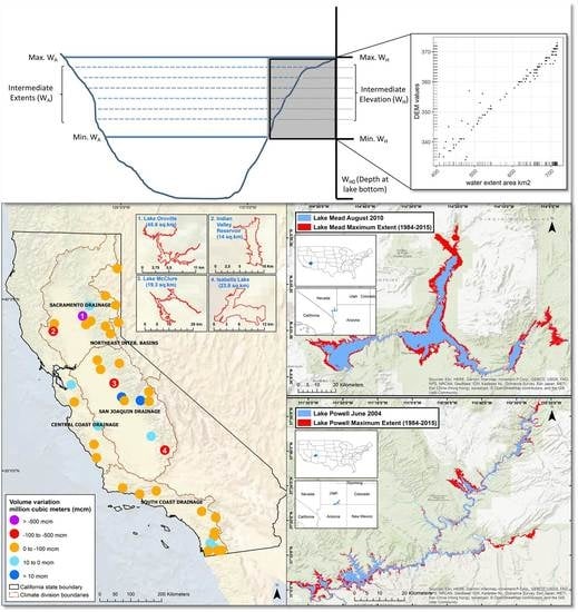
Figure 1.
Overview of Study Areas. (a) Water extent variations for validation reservoirs: Lake Mead (Top) and Lake Powell (Bottom) between 1984–2015; (b) Distribution of reservoirs in California across different climate divisions (Source: Global Reservoirs and Dam Database).
Figure 1.
Overview of Study Areas. (a) Water extent variations for validation reservoirs: Lake Mead (Top) and Lake Powell (Bottom) between 1984–2015; (b) Distribution of reservoirs in California across different climate divisions (Source: Global Reservoirs and Dam Database).

Figure 2.
Workflow: Adaptation of Area–elevation hypsometric relationship to estimate volume variations in drought prone Californian reservoirs.
Figure 2.
Workflow: Adaptation of Area–elevation hypsometric relationship to estimate volume variations in drought prone Californian reservoirs.

Figure 3.
Reservoir cross-section depicting hypsometric relationship between surface water area extent and elevation.
Figure 3.
Reservoir cross-section depicting hypsometric relationship between surface water area extent and elevation.

Figure 4.
Linear hypsometric relationship between GSW-MWH areas and median DEM values.

Figure 5.
Lake Mead volume variations.

Figure 6.
Lake Powell volume variations.

Figure 7.
Lake Mead: Relationship between estimated and in situ volume variations. The vertical lines with darker color-codes indicate the lower standard deviation of the residuals from the regression line (lower RMSE). The lighter color-codes indicate higher deviations of estimated values from the in situ values and higher RMSE.

Figure 8.
Lake Powell: Relationship between DEM estimated and in situ volume variations. The vertical lines with darker color-codes indicate the lower standard deviation of the residuals from the regression line (lower RMSE). The lighter color-codes indicate higher deviations of estimated values from the in situ values and higher RMSE.

Figure 9.
Median water volume variations in top 40 reservoirs in California between 1984–2015 based on TanDEM-X-GSW regression analysis.
Figure 9.
Median water volume variations in top 40 reservoirs in California between 1984–2015 based on TanDEM-X-GSW regression analysis.

Figure 10.
Volume variation patterns: (a) Lake Oroville, (b) Lake McClure (c) H.V. Eastman Lake (d) Hensley Lake.
Figure 10.
Volume variation patterns: (a) Lake Oroville, (b) Lake McClure (c) H.V. Eastman Lake (d) Hensley Lake.

Figure 11.
Standardized Precipitation Evapotranspiration Index on multiple time scales for San Joaquin Drainage climate division.
Figure 11.
Standardized Precipitation Evapotranspiration Index on multiple time scales for San Joaquin Drainage climate division.


Table 1.
Pearson’s correlations for multiscalar SPEI for reservoirs inside San Joaquin drainage.
| Reservoir Names | SPEI 3 Months | SPEI 6 Months | SPEI 9 Months | SPEI 12 Months | SPEI 18 Months | SPEI 24 Months | SPEI 36 Months | SPEI 48 Months | SPEI 60 Months |
|---|---|---|---|---|---|---|---|---|---|
| Lake Amador | 0.32 | 0.39 | 0.42 | 0.46 | 0.51 | 0.55 | 0.56 | 0.54 | 0.52 |
| Beardsley Reservoir | 0.3 | 0.47 | 0.54 | 0.59 | 0.51 | 0.51 | 0.46 | 0.46 | 0.37 |
| Salt Springs Valley Reservoir | 0.34 | 0.54 | 0.57 | 0.59 | 0.6 | 0.59 | 0.59 | 0.54 | 0.48 |
| Lake McClure | 0.34 | 0.51 | 0.63 | 0.7 | 0.78 | 0.75 | 0.69 | 0.61 | 0.55 |
| Lake Thomas A. Edison | 0.23 | 0.45 | 0.63 | 0.66 | 0.67 | 0.63 | 0.53 | 0.5 | 0.5 |
| H.V. Eastman Lake | 0.27 | 0.47 | 0.53 | 0.66 | 0.8 | 0.78 | 0.65 | 0.56 | 0.53 |
| Shaver Lake | 0.08 | 0.21 | 0.32 | 0.3 | 0.29 | 0.29 | 0.21 | 0.26 | 0.23 |
| Hensley Lake | 0.4 | 0.62 | 0.64 | 0.69 | 0.68 | 0.66 | 0.58 | 0.49 | 0.36 |
| Courtright Reservoir | 0.14 | 0.33 | 0.38 | 0.37 | 0.36 | 0.35 | 0.37 | 0.34 | 0.27 |
| Success Lake | 0.27 | 0.4 | 0.35 | 0.4 | 0.41 | 0.45 | 0.43 | 0.44 | 0.36 |
| Isabella lake | 0.31 | 0.51 | 0.64 | 0.71 | 0.75 | 0.71 | 0.66 | 0.62 | 0.55 |
© 2019 by the authors. Licensee MDPI, Basel, Switzerland. This article is an open access article distributed under the terms and conditions of the Creative Commons Attribution (CC BY) license (http://creativecommons.org/licenses/by/4.0/).
Share and Cite
MDPI and ACS Style
Bhagwat, T.; Klein, I.; Huth, J.; Leinenkugel, P. Volumetric Analysis of Reservoirs in Drought-Prone Areas Using Remote Sensing Products. Remote Sens. 2019, 11, 1974. https://0-doi-org.brum.beds.ac.uk/10.3390/rs11171974
AMA Style
Bhagwat T, Klein I, Huth J, Leinenkugel P. Volumetric Analysis of Reservoirs in Drought-Prone Areas Using Remote Sensing Products. Remote Sensing. 2019; 11(17):1974. https://0-doi-org.brum.beds.ac.uk/10.3390/rs11171974
Chicago/Turabian StyleBhagwat, Tejas, Igor Klein, Juliane Huth, and Patrick Leinenkugel. 2019. "Volumetric Analysis of Reservoirs in Drought-Prone Areas Using Remote Sensing Products" Remote Sensing 11, no. 17: 1974. https://0-doi-org.brum.beds.ac.uk/10.3390/rs11171974
Note that from the first issue of 2016, this journal uses article numbers instead of page numbers. See further details here.