Article

Remotely Sensed Variables of Ecosystem Functioning Support Robust Predictions of Abundance Patterns for Rare Species

by
Salvador Arenas-Castro
1,2,*,
Adrián Regos
1,3,
João F. Gonçalves
1,
Domingo Alcaraz-Segura
4,5 and
João Honrado
1,6
1
CIBIO-InBIO—Centro de Investigação em Biodiversidade e Recursos Genéticos, Laboratório Associado, Universidade do Porto, Campus Agrário Vairão, 4485-661 Vila do Conde, Portugal
2
CICGE—Centro de Investigação em Ciências Geo-Espaciais, Faculdade de Ciências, Universidade do Porto, Observatório Astronómico “Prof. Manuel de Barros”, Alameda do Monte da Virgem, 4430-146 Vila Nova de Gaia, Portugal
3
Departamento de Zooloxía, Xenética e Antropoloxía Física, Universidade de Santiago de Compostela, 15782 Santiago de Compostela, Spain
4
Department of Botany and Inter-University Institute for Earth System Research, University of Granada, 18071 Granada, Spain
5
Andalusian Center for the Assessment and Monitoring of Global Change (CAESCG), University of Almería, 04151 Almería, Spain
6
Faculdade de Ciências, Universidade do Porto, 4169-007 Porto, Portugal
*
Author to whom correspondence should be addressed.
Remote Sens. 2019, 11(18), 2086; https://0-doi-org.brum.beds.ac.uk/10.3390/rs11182086
Submission received: 7 August 2019 / Revised: 31 August 2019 / Accepted: 4 September 2019 / Published: 6 September 2019

Abstract

:
Global environmental changes are affecting both the distribution and abundance of species at an unprecedented rate. To assess these effects, species distribution models (SDMs) have been greatly developed over the last decades, while species abundance models (SAMs) have generally received less attention even though these models provide essential information for conservation management. With population abundance defined as an essential biodiversity variable (EBV), SAMs could offer spatially explicit predictions of species abundance across space and time. Satellite-derived ecosystem functioning attributes (EFAs) are known to inform on processes controlling species distribution, but they have not been tested as predictors of species abundance. In this study, we assessed the usefulness of SAMs calibrated with EFAs (as process-related variables) to predict local abundance patterns for a rare and threatened species (the narrow Iberian endemic ‘Gerês lily’ Iris boissieri; protected under the European Union Habitats Directive), and to project inter-annual fluctuations of predicted abundance. We compared the predictive accuracy of SAMs calibrated with climate (CLI), topography (DEM), land cover (LCC), EFAs, and combinations of these. Models fitted only with EFAs explained the greatest variance in species abundance, compared to models based only on CLI, DEM, or LCC variables. The combination of EFAs and topography slightly increased model performance. Predictions of the inter-annual dynamics of species abundance were related to inter-annual fluctuations in climate, which holds important implications for tracking global change effects on species abundance. This study underlines the potential of EFAs as robust predictors of biodiversity change through population size trends. The combination of EFA-based SAMs and SDMs would provide an essential toolkit for species monitoring programs.

Graphical Abstract

1. Introduction

Human-induced global environmental change is threatening biodiversity globally at an unprecedented rate [1]. These environmental changes are expected to greatly impact both the distribution and the abundance of species. In that sense, both ‘species distribution’ and ‘population abundance’ are potential candidates to be considered as essential biodiversity variables (EBVs) in the EBV class ‘species populations’ [2,3]. Predictions from species abundance models (SAMs) can deliver relevant information both on species distributions and on population sizes for biodiversity monitoring and conservation management [4]. The integration of modeling tools and biodiversity monitoring protocols has increased our capacity to quantify and anticipate the response of species to environmental change across scales [5,6,7]. Model-assisted monitoring of distribution and abundances is therefore essential to assess the effectiveness of conservation policies globally [8,9,10].
However, while species distribution models (SDMs) have been greatly developed over the last decades [11,12] (and references therein), SAMs have generally received less attention [13,14,15], but see [16] and [17,18]. Moreover, these modeling techniques have been traditionally based on climate and static habitat features [19], failing to consider other environmental information that is ecologically relevant for species. Thus, the development and application of comprehensive environmental datasets and efficient modeling techniques are needed to predict and to monitor the geographic distribution of species and abundance, along with their related environmental drivers [20]. In this regard, satellite remote sensing time-series offer continuous and cost-effective measures of the environment across space and time [21], allowing near real-time assessment of species distribution and population dynamics [22]. This is especially relevant for rare and endangered species that often hold high habitat specificity, narrow niche breadth, limited dispersal ability, and increasing habitat fragmentation.
As descriptors of exchange of matter and energy (i.e., ecosystem functioning [23,24]), and therefore processes that are key for species and their populations, satellite-derived ecosystem functioning attributes (EFAs) offer an integrative and earlier view of ecosystem responses to environmental changes than climate and landscape structural or compositional attributes [25]. Satellite-derived EFAs can, therefore, be used as process-related predictors in biodiversity models, since they provide information about ecosystem processes and properties related to the carbon (e.g., vegetation greenness) and water cycles (e.g., evapotranspiration) or with energy balance (e.g., land surface temperature and albedo). In fact, satellite-derived EFAs are being also tested as candidate EBVs related to the carbon cycle, energy, and radiation balance capable of informing about ecosystem components linked to species conservation status [26,27]. Thus, the incorporation of EFAs into SDMs was found to increase their predictive power and transferability [28], offering the opportunity to cost-effectively monitor multiple endangered species [27,29], at different spatial and temporal scales [30]. Still, despite these advantages, the predictive ability of EFAs in abundance models as well as to assess inter-annual population dynamics of rare species remains largely untested.
The main goal of this study is to assess the potential of SAMs calibrated with satellite-derived EFAs (as process-related model predictors) to predict spatial patterns of abundance and to support predictions of the inter-annual abundance dynamics for rare plants, using as test species the narrow Iberian endemic ‘Gerês lily’ (Iris boissieri; protected under the EU Habitats Directive). Furthermore, we assess whether EFAs (as EBVs from the Ecosystem function class [2]) also hold the potential to inform on species abundance dynamics (Species populations EBV class) for biodiversity monitoring and reporting [4,26]. Sequentially, we: 1) assessed the ability of satellite-derived EFAs to support reliable predictions of Iris abundance; 2) analyzed the added-value of EFAs to replace or complement ‘traditional’ climate, land cover or topographic data in species abundance models; 3) projected (through back- and fore-casting) the best model to obtain yearly abundance predictions; and 4) compared those predicted abundances with disturbance factors (fire, climate anomalies) hypothesized to explain the predicted inter-annual abundance variations. The framework proposed here is flexible enough to be applicable to other species and socio-environmental contexts globally, and it is expected to assist conservation decision-making processes related to biodiversity monitoring and reporting schemes.

2. Materials and Methods

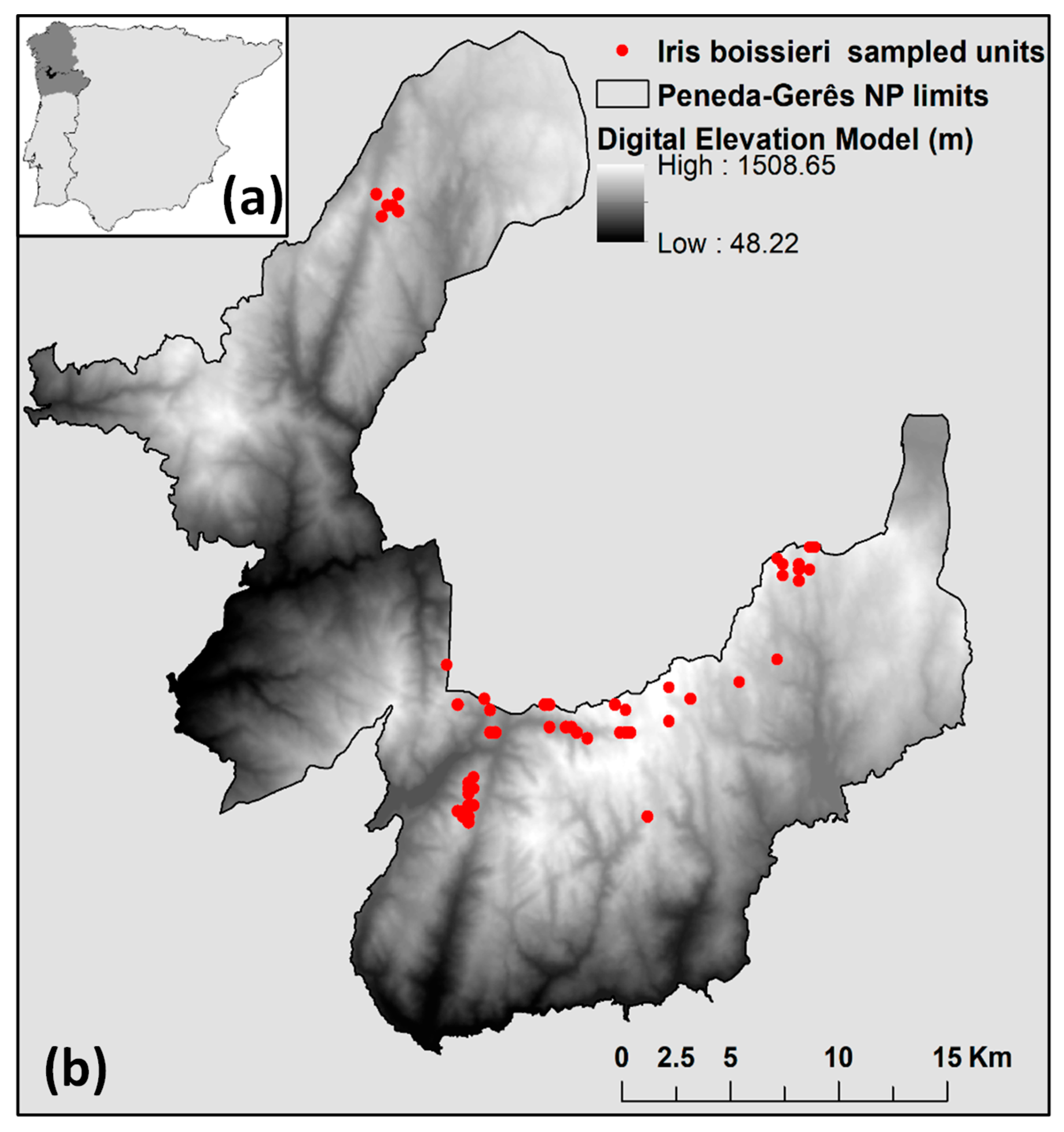
2.1. Test Species and Study Area

We tested our approach with the ‘Gerês lily’ (Iris boissieri Henriq. = Xiphion boissieri (Henriq.) Rodion), a narrow-ranged endemic plant holding a ‘critically endangered’ conservation status [31], and protected under the European Habitats Directive (hereafter HD) for which EU member-states hold regular reporting obligations (under Article 17 of the HD/Annex II and IV) [32]. This species is restricted to mountainous areas of the northwest Iberian Peninsula (Figure 1a), where Portugal concentrates the largest populations of the species, especially in the Peneda-Gerês National Park (Figure 1b). This mountain-protected area represents a transitional area between the Mediterranean and Euro-Siberian and Alpine biogeographic regions and a mosaic of mixed vegetation types characterizes it. Average annual temperatures range from 17 °C to 20 °C, with some variation along the altitudinal gradient [33]. Highlands have an average temperature of about 10 °C, ranging from 4 to 14 °C, while areas in the valleys have milder climates with an average temperature of 14 °C, ranging from 8 to 20 °C. Total mean rainfall reaches 3000 mm per year (with more than 130 rainy days per year) and snowfall is frequent in the mountaintops.
The highest rocky outcrops with steep topography and low accessibility are the main habitat for the ‘Gerês lily’ [31]. The species typically occurs in open scrublands and crevices of granite outcrops at elevations between 500 and 1500 m above sea level. Many of these habitat areas were maintained by the traditional grazing system, which involved frequent small-scale burning for pasture maintenance and was therefore an important control of vegetation encroachment. This long-term land management system has been declining for decades due to severe rural depopulation and other socioeconomic changes. As a result, widespread vegetation encroachment has changed habitat conditions as well as the local fire regime, potentially affecting the conservation of Iris boissieri and other plant species of high conservation concern.

2.2. Species Abundance Dataset

The original dataset consisted of abundance estimates (counts of the number of individuals), performed in situ in the Peneda-Gerês National Park (Portugal) in 2006 by Park botanists. The field survey was conducted by visiting all previously known Iris occurrence sites as well as the neighboring areas. Iris clusters separated from each other by more than 100 meters were considered as distinct local populations to perform the counts.
To match abundance data to the EFAs resolution (ca. 232 m MODIS pixel size; see below), abundance values were aggregated for each cell following an area-proportional allocation rule, i.e., the total number of plants within each sampling area (i.e., a local population defined by a polygon) was split between contiguous grid cells depending on the proportionally occupied area by the polygon in each cell. The final abundance dataset consisted of 61 cells (of the 232 m grid; Figure 1b), with the number of Iris plants per cell ranging from 1 to 285.

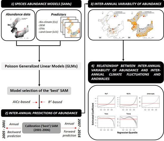
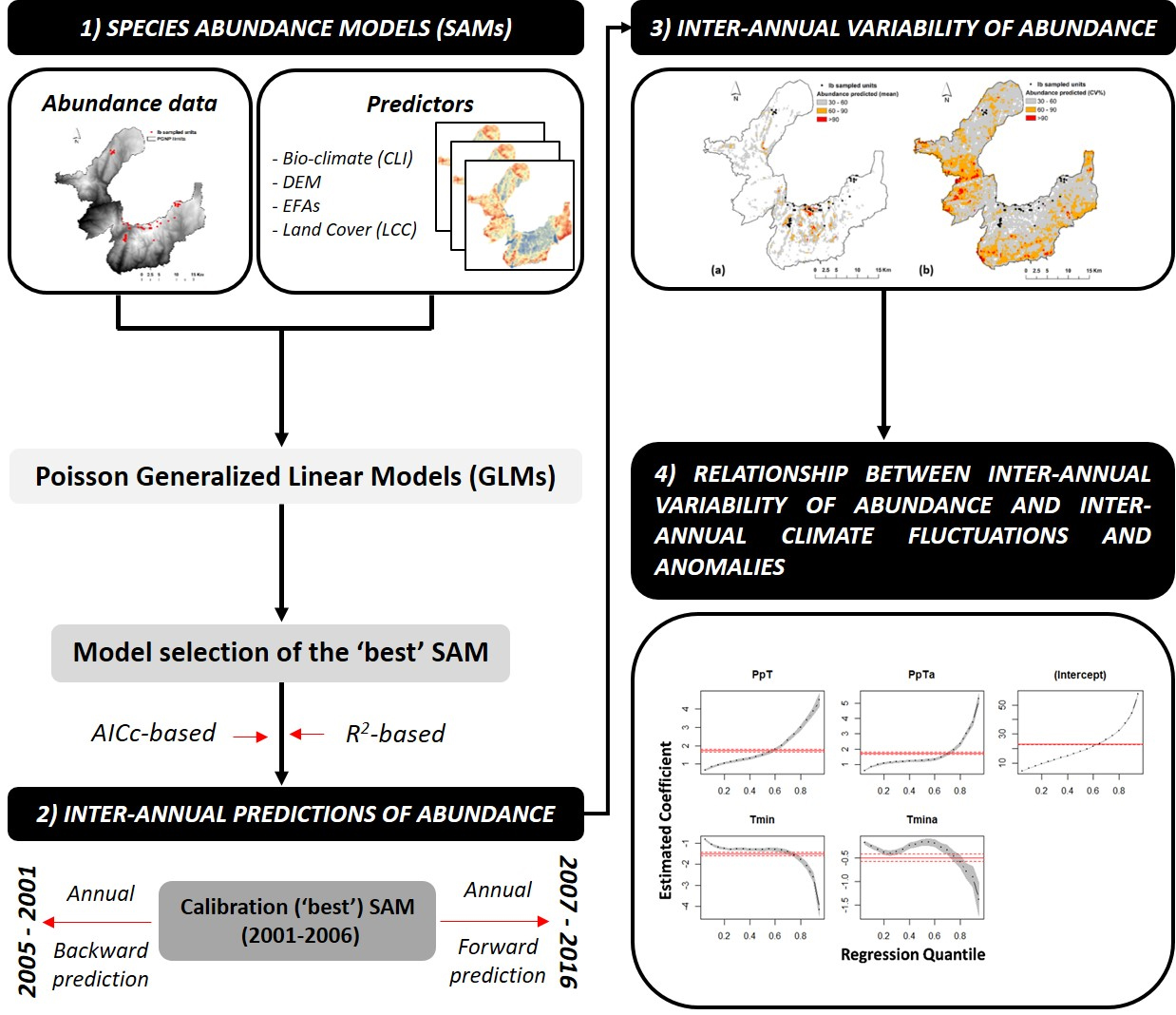
2.3. Modeling Framework

To assess the predictive ability of satellite-derived EFAs in abundance models, we compared SAMs based on EFAs against SAMs based on climatic, topographic, or landscape variables. The best predictors were then combined to test whether more robust SAMs (and thus better abundance predictions) could be obtained.

2.3.1. Environmental Predictors

We selected candidate predictive variables expressing environmental and ecological factors that are known to influence plant physiology, distribution, and local habitat preferences over a period (details below) as close as possible to the date of the in-situ abundance survey (2006).
Based on a monthly time series of air temperature (mean maximum and mean minimum temperature) and total precipitation—which were calculated from meteorological stations in Spain and Portugal by using multiple regression techniques (see details in [34])—we derived 19 (bio-) climate variables at 200 m spatial resolution for each year from 2000 to 2010 by using the function ‘biovars’ available in the R package ‘dismo’, version 1.1.
Land use/cover data was obtained by a hybrid classification procedure of Landsat-7 ETM + optical and thermal imagery (19 May 2010 and 30 July 2010; 30 m resolution), which combines unsupervised and supervised techniques (see details in [28]). From the classified land cover/use maps, we obtained the fractional cover of forest, shrubland, and rocky outcrop types to use as landscape composition variables at a spatial resolution of 232 m.
From the digital elevation model (DEM) over Europe (EU-DEM based on SRTM and ASTER GDEM; https://www.eea.europa.eu/data-and-maps/data/eu-dem) produced at 30 m resolution, we derived topographic variables at 232 m grid size by using the function ‘terrain’ available in the R package ‘raster’, version 2.8–19.
To compute EFAs, we used the MODIS Enhanced Vegetation Index (EVI) (MOD13Q1.v006; 232 m pixel every 16 days) for the 2001–2016 period. For that, we used Google Earth Engine [35] to derive the following eight summary metrics of the EVI seasonal dynamics: EVI annual mean (surrogate of annual primary production), EVI annual maximum and minimum (indicators of the annual extremes), EVI seasonal standard-deviation (descriptor of seasonality), and sine and cosine of the dates of maximum and minimum EVI [25,36] (indicators of phenology).
All environmental variables were processed to match the pixel size to the EFAs resolution (ca. 232 m grid size) at the geographical coordinate system WGS84, using the R package ‘raster’ (version 2.8–19). The initial dataset included 44 candidate predictors (Table S1—Supporting Information). To avoid including highly correlated variables in model fitting, we conducted a multicollinearity analysis by testing Pearson pair-wise correlations and Variance Inflation Factors (VIF). Based on these multicollinearity analyses, we finally retained three independent predictors for each competing model (with Pearson’s correlation coefficients of < 0.7 and VIF of < 4; Table S2; Figure S1).

2.3.2. Model Fitting

For each model, the response variable (Iris abundance per grid cell; 61 records) was related to predictor variables using generalized linear models (GLMs) calibrated with three predictors. GLMs are flexible statistical methods for analyzing ecological relationships since they take into account the interactive behavior of variables that can be poorly represented by classical Gaussian (linear) distributions [37]. Furthermore, recent literature recommends using models based on Poisson and negative binomial distributions instead of log-transforming the data [38] with the main advantage that the parameters are estimated on the original scale and thus back-transformations are avoided [39]. Since this is an increasingly-used approach for count (abundance) data, we related Iris abundance values to predictors by computing a negative binomial distribution of errors (after checking for overdispersion effects in Poisson models and robust estimation via weighted likelihood), and applying a logarithmic link function by using the function ‘glm.nb’ available in the R package ‘MASS’, version 7.3–51.1. Based on a multi-model inference (MMI) framework [40], we tested and ranked the individual competing models fitted with three variables for abundance predictions performance (Table S2).
We calibrated five GLMs as follows: (1) models based on process-related (i.e., ecosystem functioning) predictors (‘EFA’)—using only remotely sensed EFAs (their inter-annual mean for the 2001–2006 period); (2) climate-based models (‘CLI’)—using variables extracted from the monthly climate dataset (the inter-annual mean for the 2000–2010 period); (3) models based on land cover (landscape composition) predictors (‘LCC’)—from land cover maps (year 2010); (4) models based on topographic variables (‘DEM’); and (5) a best model, combining the most significant three predictors selected from all possible combinations of previous groups. The Akaike Information Criterion with a correction for finite sample size (AICc) was used to rank the competing models [41]. Complementarily, we used the explained deviance and Spearman’s correlation between observed and predicted values to assess model fitting. Models that were not significant, or with low performance in AICc or in explained deviance were excluded from the analysis. We also tested the predictive accuracy of each model by calculating the mean absolute scaled error (MASE) [42]. A MASE higher than 1 implies that the actual forecast is worse than a naive forecast as a reference method calculated as a sample, while a MASE lower than 1 implies that the current forecast behavior is better than the naive method. For that, we used the ´accuracy´ function through the R package ´forecast´ (version 8.9).

2.4. Inter-Annual Predictions of Iris Abundance

The best model was backcasted and forecasted (i.e., projected) to the environmental conditions of each year to obtain a time-series of annual abundance predictions. Specifically, we used the most parsimonious and with greater predictive accuracy (‘best’) SAM (the one calibrated with the inter-annual (2001–2006) average values of EFAs plus topography; see Results) to obtain annual backward (from 2005 to 2001) and forward (from 2007 to 2016) yearly projections. We also calculated the inter-annual mean (̄X̄), the inter-annual standard deviation (SD), and the inter-annual coefficient of variation (CV; %) of predicted abundance at the grid cell level for the entire 2001–2016 time-period as a spatiotemporal proxy of the inter-annual variability of Iris populations.
Finally, we explored possible relations between the inter-annual variability of species predicted abundance and the occurrence of disturbances, namely those related to fire and climate, by applying quantile regression analysis. Unlike ordinary least square regression, quantile regression is a distribution-agnostic methodology, which makes no assumptions about the distribution of the residuals, and therefore not assume a parametric distribution for the response [43]. Thus, we explored different aspects of the relationship (as signals and effects) between the dependent variable (predicted abundance) and the independent variables (climate variables and anomalies). To do so, we calculated the total burned area per year from official wildfire maps based on Landsat-7 ETM+ images [44] for the 2001–2016 period. Climatic means and annual anomalies were derived from TerraClimate [45] at 4 km resolution for the same period: total annual precipitation (mm·year−1, PpT); average annual minimum temperature (°C; Tmin); and average annual maximum temperature (°C; Tmax). Since climate data, in general, have much more spatial autocorrelation, we resampled these climatic variables to ca. 232 m.
The Iris abundance values showed a right-skewed distribution, and a prevalence of low abundance values makes it difficult to extract relations between population size and predictors in abundance trend analysis (heteroskedastic response [46,47]). To check the relationships and signals between the response variable (predicted abundance) and independent variables (climate and its anomalies), we applied quantile regression tests (‘quantreg’ R package) fitted to the median (quantile = 0.5). To test the goodness-of-fit for quantile regression models, we used the pseudo-R2 measure suggested by [48]. Furthermore, we tested the same associations between inter-annual predicted abundances and fire and climate variables, but for different levels of population size (quantiles). For that, we applied the same quantile regression test where abundances were separated by 5% intervals (i.e., in quantiles) in order to overcome limitations related to the right-skewed distribution and heteroskedastic response of abundance data. To check significant differences across quantiles, we used the test of equality of slopes by using the ´ANOVA´ function implemented by ‘quantreg’ developers.
All analyses were conducted using the R environment for statistical computation [49]. QGIS version 2.18.11 and ArcGIS version 10.2 were used for managing and representing spatial data and projections.

3. Results

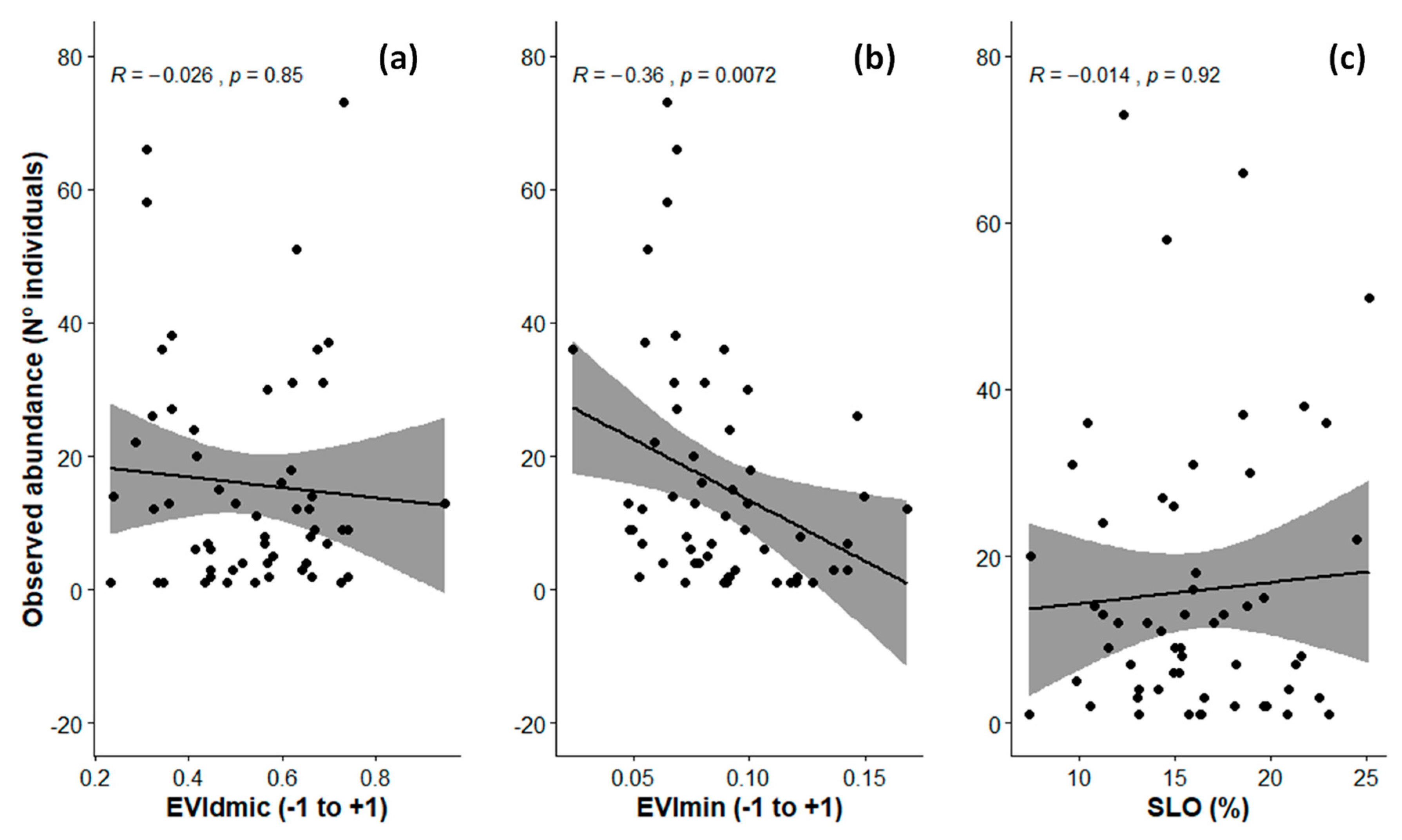
3.1. Ranking of Models and Predictors

Overall, models that include EFAs as predictors showed the highest performance (explained deviance up to 0.3), whereas the LCC-based model attained the lowest performance (Table 1).
The most parsimonious model (based on AICc) and with the greatest predictive ability (based on MASE) was obtained when combining EFAs and topographic variables (EFAs + DEM model; Table 1). The correlation between species abundance and predictor variables in this model (EVIdmic, EVImin, and SLO) was negative for the two EFAs and positive for SLO (Spearman correlations were −0.13, −0.37, and 0.10, respectively); however, only EVImin showed a significant correlation with Iris abundance (Figure 2).

3.2. Inter-Annual Variability of Iris Abundance

On average (considering all pixels in the study area), the median and median absolute deviation (MAD) of abundance predictions based on EFAs projections over the full 2001–2016 time-period were of 17.43 (12 for observed values) and 12.04 (14.08) individuals, respectively, ranging from 12.79 (11.96 MAD) in year 2006 to 23.85 (11.84 MAD) in year 2007 (Figure S2). Overall, the inter-annual abundance predictions were spatially consistent with the known locations of Iris (Figure S3).
The inter-annual mean of the predicted abundances for the 61 observed sampled cells based on the predicted spatial X̄, SD and CV were 25.02, 8.06 and 33.06 individuals, respectively. Spearman correlation analysis showed a high and positive significant correlation between the X̄ and SD (r = 0.83, p < 0.05) (Figure S4). There was also a high correlation of X̅ with slope (r = 0.81, p < 0.05) and with EVImin (r = −0.33, p < 0.05), but no correlation with EVIdmic. The CV showed no correlation with slope (r = −0.07, p < 0.05), but a correlation with EVImin (r = 0.60, p < 0.05) and EVIdmic (r = −0.23, p < 0.05). Those grid cells that combine higher values for the X̄, and lower values for the CV, therefore represent those areas where conditions are better to maintain large populations (Figure 3a,b).
The overall mean for the study area of the annual predicted abundance matched the indicator of minimum photosynthetic activity (EVImin) (Figure 4a), and was higher after rainy years (total average annual precipitation; PpT), and mainly matched chilly years (lower values of maximum (Tmax) and minimum (Tmin) annual temperature) (Figure 4b). More specifically, climate conditions of the year with the lowest predicted abundance (16.79; 2002) were PpT = 1724.97 mm·year−1, Tmax = 15.69 °C, and Tmin = 7.38 °C, while for the year with the largest predicted abundance (23.85; 2007) were PpT = 1087.49 mm year-1, Tmax = 15.88 °C, and Tmin = 7.21 °C. However, wildfires (total burnt area; TBA) did not have a significant effect on predicted Iris abundances (R1 (pseudoR2) = 0.025; Figure 4c; Figure S5).
The quantile regression analysis between average annual predicted abundance and inter-annual climate fluctuations (in abundance levels across time), and anomalies (changes in climatic variables in relation to the mean), showed negative relationships for total precipitation (PpT; R1 (pseudoR2) = 0.30), and its anomalies (PpTa; R1 = 0.30), as well as minimum temperature (Tmin; R1 = 0.27) and its anomalies (Tmina; R1 = 0.28) (Figure S6).
Quantile regression analyses showed that climate variables and anomalies affected species abundances differently depending on the levels of Iris abundance (Figure 5). Regression models revealed a heteroskedastic response with overall greater effect sizes occurring for larger populations (F = 148.32 ***). In particular, precipitation (PpT) and its anomalies (PpTa) have a positive effect on species abundance, but especially at the highest levels of abundance (Figure 5; Table 2) and for specific climate restrictions, i.e., below the average PpT (1416.88 mm·year−1) and average Tmin (7.38 °C) (Figure 4b). Conversely, the minimum temperature (Tmin) and its anomalies (Tmina) negatively affected species abundances, also especially for higher values of abundance (see from quantile 0.75 in Figure 5).

4. Discussion

Based on the promising performance of satellite-derived ecosystem functioning attributes (EFAs) to predict species distributions [27,30,50], here we tested the potential of EFAs as robust process-related predictors of population size for a rare (and critically endangered) plant species. Overall, species abundance models (SAMs) fitted only with EFAs provided the greatest explained variance of species abundance compared to models based only on climate, land cover, or topography variables. The combination of EFAs and topography slightly increased the model performance (“best model”). In addition, the inter-annual abundance predictions based on EFAs provided high performance as potential indicator of population variability and/or stability of target species. Our results also showed positive relations between predictions of the inter-annual species abundance dynamics and inter-annual climate fluctuations and anomalies, suggesting a potential early-warning signal for global change impacts on species abundance, consistent with previous reports for species distributions [27]. In summary, this study provides new insights on the usefulness of EFAs as integrative and dynamic predictors for tracking and forecasting biodiversity changes, which is an advantage for implementing or improving species monitoring programs fed by EO data.

4.1. Ecosystem Functioning Attributes as Predictors in Species Abundance Models

We found that models fitted with EFAs measured from satellite remote sensing supported more robust (or at least as robust) predictions of species abundance than models based on climate, topography, or land cover (Table 1). In addition, satellite-derived EFAs hold the advantage of being frequently and easily updated. Overall, these results confirm the ability of EFAs to support reliable predictions of abundance for rare species (such as I. boissieri) at high spatial and temporal resolutions, and they stand up as promising integrative predictors not only in species distribution models [30], but also in species abundance models. Our most parsimonious model, combining EFAs and topographic features, supports the use of satellite-derived products as continuous and integrative measures of biotic and abiotic factors across space and time, hardly quantifiable by other means. This “best model” revealed that the local abundance of this narrow-ranged species is mainly influenced by the minimum green-up days of the year related to late winter–early spring (EVIdmic; Figure 2a), and by low productivity during the winter–early spring (EVImin; Figure 2b), which is linked to sparsely vegetated landscape mosaics dominated by crawling scrub and grasslands. In addition, abundance rates showed a slight increase with steeper slopes (Figure 2c). These results match previous ecological knowledge of the species [31] since it is most often found in steep, high elevation areas.
Our results also showed that climate is per se not a good predictor of the species abundance in space [13,51], but a good one in time, suggesting that other non-climatic (but climate-driven) factors might be influencing the abundance levels of the species at the focal spatial resolution [52,53]. Climate models fitted by interpolated data from meteorological stations are greatly influenced by the spatial scale [54,55], while remote sensing (RS) factors such as EFAs and topography (e.g., SLO) are more direct measurements of landscape conditions [56,57]. However, climate did show a close relation with yearly predictions of species abundance, as well as EFAs, since both capture properly the temporal dynamics of environmental conditions [58]. Conversely, structural predictors derived from RS-LCC maps hold limitations since they have inadequate spatial, thematic and/or temporal resolutions for the species’ dynamics [27].
Predictors related to productivity and phenology were the most important in EFA-based models, consistently with SDM predictions (e.g., [30]), suggesting that remotely-sensed descriptors of the carbon cycle were capable of capturing relevant aspects of ecosystem functioning for explaining species abundance, as already suggested for plant and bird distributions [27,28,30]. These results therefore support the idea that EFAs capture an integrative response to multiple environmental drivers since not only showed a similar or better performance than climate or land-cover composition, but also to the combination of them [30,59]. In addition, the combination of EFAs and other RS-derived factors (such as topography) significantly increased model performance, further highlighting the need to integrate descriptors of ecosystem functioning into species abundance models to improve biodiversity monitoring [27,28,30].

4.2. Inter-Annual Variability of Species Abundance and its Driving Forces

Overall, the inter-annual predictions of abundance were within a reasonable range of values and showed spatial consistency with the areas where the focal species was actually observed (Figure 3). Indeed, inter-annual EFA-based abundance predictions are congruent with previous research predicting habitat suitability for this narrow-ranged species [30]. As expected, grid cells with topographic features such as small depressions with an accumulation of coarse deposits and crevices of granite outcrops above 800–900 m, dominated by open vegetation formed by grasses and low scrubs and showing the low EVI values, had the highest predicted abundance values on average for the whole time period (Figure 3a). These grid cells with the greatest predicted abundance in terms of inter-annual mean and lowest inter-annual coefficient of variation should be the ones holding the most stable areas for Iris abundance. Therefore, inter-annual satellite-derived EFAs were able to improve our understanding of the spatial and temporal variability of species abundance, supporting the view that EFA-based abundance predictions can allow significant improvements to a far wider variety of applications beyond distribution or habitat suitability maps [13,22,60].
Once confirmed the potential of ecosystem functioning attributes for predicting (spatially and temporally) Iris abundances, we compared the inter-annual EFA-based predicted abundance variations with the occurrence of disturbance factors (such as climate anomalies and burned area). This assessment would help to monitor population sizes in space and time at finer scales, thereby improving the effectiveness of management actions on the ground. Among the associations between the EFA-based predicted relative abundance for each year and factor, only three climate-related models were statistically significant (Figure S6). Our results revealed that precipitation (PpT) and its positive anomalies (PpTa) potentially increase the abundance of the species (Figure 5), especially at the highest levels of abundance, while the minimum temperature (Tmin) and its anomalies (Tmina) negatively affected the species’ abundance, also mainly for higher abundance values. These results matched with the rather specific environmental conditions under which Iris thrives, under cool temperatures and high precipitation values. However, the life-form of Iris is a bulbous geophyte that remains in a latent state during the less-favorable season. Therefore, a balance between humidity (high enough so that the bulb does not die due to water stress) and temperature (not too low so the bulb does not freeze) would be suitable conditions for plant survival.
We found no association between total burned area and Iris abundance (Figure S5). However, the highest abundance values seemed to be predicted for 1–2 years after large burned areas, which might be explained by a biological lag-response of the species to fire (years 2004, 2007, 2012, and 2015 in Figure 4c). Fire may directly cause plant mortality, but low-severity fires also provide open spaces and an opportunity for the species by encouraging sprouting, reducing interspecific competition, and increasing sunlight availability [61,62].
Our results also showed significant differences between low and high abundance groups (quantiles) regarding the effect of precipitation and temperature on population size, especially in the case of anomalies, which is consistent with the ecophysiological effect of these variables on plant species. These findings showed that the annual variability in climate was consistent with the annual fluctuations of EFA-based predicted abundances. Since this implies that larger populations will likely be more affected by projected changes in climate, these results hold important implications for detecting early warnings of species abundance change and to support effective decisions on future conservation in the face of global change [63].

5. Conclusions

In conclusion, our findings confirm the potential of ecosystem functioning attributes (EFAs) derived from satellite remote sensing as predictors of local abundance for rare plant species. Our results also demonstrate that EFAs provide spatially and temporally valuable information on the variability and/or stability of species population sizes, and not only concerning the distribution of species and habitats, which can be used for planning effective management actions. This reinforces local population size as candidate EBV (‘population abundance’) and EFAs as meaningful EBVs of ecosystem function that can be implemented in EFA-based SAMs for reporting and monitoring species conservation status (e.g., ETC/BD 2011). Since complying with the legal obligations of EU member-states under Article 17th of the Habitats Directive requires providing extensive data on relevant parameters or indicators (e.g., range, number and dimension of populations, suitable habitat, and future prospects), we strongly emphasize the importance of incorporating descriptors of inter-annual ecosystem functioning and dynamics in conservation monitoring and planning.

Supplementary Materials

The following are available online at https://0-www-mdpi-com.brum.beds.ac.uk/2072-4292/11/18/2086/s1, Figure S1: Correlation matrix (a) and variance inflation factors (VIF) plot (b) for variables used in model fitting. Figure S2: Frequencies of predicted abundance per year for the period 2001–2016. Red line shows the median of the distribution values. Figure S3: Inter-annual spatial variability of the predicted abundance of Iris boissieri based on ecosystem functional attributes (EFAs). Figure S4: Correlation matrix between the mean, the standard-deviation, and the coefficient of variation of predicted abundance (Prjm, Prjsd, and Prjcv, respectively), and the three predictors included in model fitting (EVImin, EVIdmic, and SLO). Figure S5: Quantile regression plot fitted to the median (quantile = 0.5) representing the relation sign between the annual mean of predicted abundance, aggregated by year, and the averaged total burned area (TBA). Figure S6: Quantile regression plots fitted to the median (quantile = 0.5) representing the relation sign between the annual mean of predicted abundance, aggregated by year, and the average of each climatic variable (and anomalies) for the whole study area. Table S1: Summary of the full sets of predictors used to calibrate abundance models. Table S2: Final sets of predictors used to calibrate GLMs for Iris abundance in the Peneda-Gerês National Park.

Author Contributions

Conceptualization: S.A.-C., J.H.; data curation: S.A.-C., A.R., and D.A.-S.; formal analysis: S.A.-C., A.R., J.F.G., D.A.-S., and J.H.; investigation: S.A.-C.; methodology, S.A.-C., A.R., J.F.G., and D.A.-S.; software: S.A.-C., A.R., J.F.G., and D.A.-S.; visualization: S.A.-C.; funding acquisition: J.H.; resources: D.A.-S. and J.H.; supervision: J.H.; writing—original draft preparation, S.A.-C. All authors supported paper writing—review and editing.

Funding

This work has been carried out within the H2020 project ECOPOTENTIAL: Improving Future Ecosystem Benefits Through Earth Observations (http://www.ecopotential-project.eu). The project has received funding from the European Union’s Horizon 2020 research and innovation program under grant agreement No. 641762. S.A.-C., D.A.-S., and J.H. received funding from the ECOPOTENTIAL project. A.R. was financially supported by the Xunta de Galicia, Spain (post-doctoral fellowship ED481B2016/084-0). J.F.G. was funded by the Individual Scientific Employment Stimulus Program (2017) by the Portuguese Foundation for Science and Technology (FCT CEEC-2017).

Acknowledgments

The authors would like to thank Paulo Alves for the technical support on fieldwork databases.

Conflicts of Interest

The authors declare no conflict of interest.

References

  1. IPBES. The Intergovernmental Science-Policy Platform on Biodiversity and Ecosystem Services; IPBES: Paris, France, 2019. [Google Scholar]
  2. Pereira, H.M.; Ferrier, S.; Walters, M.; Geller, G.N.; Jongman, R.H.G.; Scholes, R.J.; Bruford, M.W.; Brummitt, N.; Butchart, S.H.M.; Cardoso, A.C.; et al. Essential Biodiversity Variables. Science 2013, 339, 277–278. [Google Scholar] [CrossRef] [Green Version]
  3. Pereira, H.; Belnap, J.; Böhm, M.; Brummitt, N.; Garcia-Moreno, J.; Gregory, R.; Martin, L.; Peng, C.; Swaay, V.P.; Schmeller, D.; et al. Monitoring essential biodiversity variables at the species level. In The GEO Handbook on Biodiversity Observation Networks; Walters, M., Scholes, R., Eds.; Springer: Berlin/Heidelberg, Germany, 2017. [Google Scholar]
  4. Kissling, W.D.; Ahumada, J.A.; Bowser, A.; Fernandez, M.; Fernández, N.; García, E.A.; Guralnick, R.P.; Isaac, N.J.B.; Kelling, S.; Los, W.; et al. Building essential biodiversity variables (EBVs) of species distribution and abundance at a global scale. Biol. Rev. 2018, 93, 600–625. [Google Scholar] [CrossRef]
  5. Nielsen, S.E.; Johnson, C.J.; Heard, D.C.; Boyce, M.S. Can models of presence-absence be used to scale abundance? Two case studies considering extremes in life history. Ecography 2005, 28, 197–208. [Google Scholar] [CrossRef]
  6. Elith, J.; Leathwick, J.R. Species distribution models: ecological explanation and prediction across space and time. Annu. Rev. Ecol. Evol. Syst. 2009, 40, 677–697. [Google Scholar] [CrossRef]
  7. Van Couwenberghe, R.; Collet, C.; Pierrat, J.-C.; Verheyen, K.; Gégout, J.-C. Can species distribution models be used to describe plant abundance patterns? Ecography 2013, 36, 665–674. [Google Scholar] [CrossRef]
  8. Scholes, R.J.; Walters, M.; Turak, E.; Saarenmaa, H.; Heip, C.H.; Tuama, É.Ó.; Faith, D.P.; Mooney, H.A.; Ferrier, S.; Jongman, R.H.; et al. Building a global observing system for biodiversity. Curr. Opin. Environ. Sustain. 2012, 4, 139–146. [Google Scholar] [CrossRef]
  9. Tittensor, D.P.; Walpole, M.; Hill, S.L.L.; Boyce, D.G.; Britten, G.L.; Burgess, N.D.; Butchart, S.H.M.; Leadley, P.W.; Regan, E.C.; Alkemade, R.; et al. A mid-term analysis of progress toward international biodiversity targets. Science 2014, 346, 241–244. [Google Scholar] [CrossRef]
  10. Honrado, J.P.; Pereira, H.M.; Guisan, A. Fostering integration between biodiversity monitoring and modelling. J. Appl. Ecol. 2016, 53, 1299–1304. [Google Scholar] [CrossRef]
  11. Araújo, M.B.; Guisan, A. Five (or so) challenges for species distribution modelling. J. Biogeogr. 2006, 33, 1677–1688. [Google Scholar] [CrossRef]
  12. Zimmermann, N.E.; Edwards, T.C., Jr.; Graham, C.H.; Pearman, P.B.; Svenning, J.-C. New trends in species distribution modelling. Ecography 2010, 33, 985–989. [Google Scholar] [CrossRef]
  13. Howard, C.; Stephens, P.A.; Pearce-Higgins, J.W.; Gregory, R.D.; Willis, S.G. Improving species distribution models: the value of data on abundance. Methods Ecol. Evol. 2014, 5, 506–513. [Google Scholar] [CrossRef] [Green Version]
  14. Ehrlén, J.; Morris, W.F. Predicting changes in the distribution and abundance of species under environmental change. Ecol. Lett. 2015, 18, 303–314. [Google Scholar] [CrossRef]
  15. Jetz, W.; McGeoch, M.A.; Guralnick, R.; Ferrier, S.; Beck, J.; Costello, M.J.; Fernandez, M.; Geller, G.N.; Keil, P.; Merow, C.; et al. Essential biodiversity variables for mapping and monitoring species populations. Nat. Ecol. Evol. 2019, 3, 539–551. [Google Scholar] [CrossRef] [Green Version]
  16. Ives, A.R. Predicting the response of populations to environmental change. Ecology 1995, 76, 926–941. [Google Scholar] [CrossRef]
  17. Mutshinda, C.M.; O’Hara, R.B.; Woiwod, I.P. What drives community dynamics? Proc. R. Soc. B Biol. Sci. 2009, 276, 2923–2929. [Google Scholar] [CrossRef] [Green Version]
  18. Mutshinda, C.M.; O’Hara, R.B.; Woiwod, I.P. A Multispecies perspective on ecological impacts of climatic forcing. J. Anim. Ecol. 2011, 80, 101–107. [Google Scholar] [CrossRef]
  19. Oliver, T.H.; Morecroft, M.D. Interactions between climate change and land use change on biodiversity: Attribution problems, risks, and opportunities. Wiley Interdiscip. Rev. Clim. Chang. 2014, 5, 317–335. [Google Scholar] [CrossRef]
  20. Lomolino, M.V.; Riddle, B.R.; Whittaker, R.J. (Eds.) Biogeography, 5th ed.; Oxford University Press: Sunderland, MA, USA, 2017. [Google Scholar]
  21. He, K.S.; Bradley, B.A.; Cord, A.F.; Rocchini, D.; Tuanmu, M.-N.; Schmidtlein, S.; Turner, W.; Wegmann, M.; Pettorelli, N. Will remote sensing shape the next generation of species distribution models? Remote Sens. Ecol. Conserv. 2015, 1, 4–18. [Google Scholar] [CrossRef] [Green Version]
  22. Pettorelli, N.; to Bühne, H.; Tulloch, A.; Dubois, G.; Macinnis-Ng, C.; Queirós, A.M.; Keith, D.A.; Wegmann, M.; Schrodt, F.; Stellmes, M.; et al. Satellite remote sensing of ecosystem functions: Opportunities, challenges and way forward. Remote Sens. Ecol. Conserv. 2018, 4, 71–93. [Google Scholar] [CrossRef]
  23. Jax, K. (Ed.) Ecosystem Functioning; Cambridge University Press: Cambridge, UK, 2010. [Google Scholar] [CrossRef]
  24. Cabello, J.; Fernández, N.; Alcaraz-Segura, D.; Oyonarte, C.; Piñeiro, G.; Altesor, A.; Delibes, M.; Paruelo, J.M. The ecosystem functioning dimension in conservation: Insights from remote sensing. Biodivers. Conserv. 2012, 21, 3287–3305. [Google Scholar] [CrossRef]
  25. Mouillot, D.; Graham, N.A.J.; Villéger, S.; Mason, N.W.H.; Bellwood, D.R. A functional approach reveals community responses to disturbances. Trends Ecol. Evol. 2013, 28, 167–177. [Google Scholar] [CrossRef]
  26. Pettorelli, N.; Wegmann, M.; Skidmore, A.; Mücher, S.; Dawson, T.P.; Fernandez, M.; Lucas, R.; Schaepman, M.E.; Wang, T.; O’Connor, B.; et al. Framing the concept of satellite remote sensing essential biodiversity variables: Challenges and future directions. Remote Sens. Ecol. Conserv. 2016, 2, 122–131. [Google Scholar] [CrossRef]
  27. Alcaraz-Segura, D.; Lomba, A.; Sousa-Silva, R.; Nieto-Lugilde, D.; Alves, P.; Georges, D.; Vicente, J.R.; Honrado, J.P. Potential of satellite-derived ecosystem functional attributes to anticipate species range shifts. Int. J. Appl. Earth Obs. Geoinf. 2017, 57, 86–92. [Google Scholar] [CrossRef]
  28. Regos, A.; Gagne, L.; Alcaraz-Segura, D.; Honrado, J.P.; Domínguez, J. Effects of species traits and environmental predictors on performance and transferability of ecological niche models. Sci. Rep. 2019, 9, 4221. [Google Scholar] [CrossRef]
  29. Requena-Mullor, J.M.; López, E.; Castro, A.J.; Alcaraz-Segura, D.; Castro, H.; Reyes, A.; Cabello, J. Remote-sensing based approach to forecast habitat quality under climate change scenarios. PLoS ONE 2017, 12, e0172107. [Google Scholar] [CrossRef]
  30. Arenas-Castro, S.; Goncalves, J.; Alves, P.; Alcaraz-Segura, D.; Honrado, J.P. Assessing the multi-scale predictive ability of ecosystem functional attributes for species distribution modelling. PLoS ONE 2018. [Google Scholar] [CrossRef]
  31. Ortiz, S.; Pulgar Sañudo, I. Iris Boissieri. In The IUCN Red List of Threatened Species 2011; IUCN: Cambridge, UK, 2011. [Google Scholar]
  32. Evans, D.; Arvela, M. Assessment and reporting under article 17 of the habitats directive. In Explanatory Notes & Guidelines for the period 2007–2012; European Commission: Brussels, Belgium, 2011. [Google Scholar]
  33. Plano de Ordenamento Do Parque Nacional Da Peneda-Gerês. 2010. Available online: http://www2.icnf.pt/portal/florestas/dfci/inc/info-geo (accessed on 5 August 2019).
  34. Ninyerola, M.; Pons, X.; Roure, J.M. A methodological approach of climatological modelling of air temperature and precipitation through GIS techniques. Int. J. Climatol. 2000, 20, 1823–1841. [Google Scholar] [CrossRef]
  35. Gorelick, N.; Hancher, M.; Dixon, M.; Ilyushchenko, S.; Thau, D.; Moore, R. Google earth engine: Planetary-scale geospatial analysis for everyone. Remote Sens. Environ. 2017, 202, 18–27. [Google Scholar] [CrossRef]
  36. Alcaraz-Segura, D.; Cabello, J.; Paruelo, J.M.; Delibes, M. Use of descriptors of ecosystem functioning for monitoring a national park network: A remote sensing approach. Environ. Manag. 2009, 43, 38–48. [Google Scholar] [CrossRef]
  37. Guisan, A.; Edwards, T.C.; Hastie, T. Generalized linear and generalized additive models in studies of species distributions: Setting the scene. Ecol. Modell. 2002, 157, 89–100. [Google Scholar] [CrossRef]
  38. O’Hara, R.B.; Kotze, D.J. Do not log-transform count data. Methods Ecol. Evol. 2010, 1, 118–122. [Google Scholar] [CrossRef] [Green Version]
  39. St-Pierre, A.P.; Shikon, V.; Schneider, D.C. Count data in biology-data transformation or model reformation? Ecol. Evol. 2018, 8, 3077–3085. [Google Scholar] [CrossRef]
  40. Symonds, M.R.; Moussalli, A. A brief guide to model selection, multimodel inference and model averaging in behavioural ecology using akaike’s information criterion. Behav. Ecol. Sociobiol. 2011, 65, 13–21. [Google Scholar] [CrossRef]
  41. Burnham, K.; Anderson, D. Model Selection and Multimodel Inference: A Practical Information-Theoretic Approach; Springer: Berlin/Heidelberg, Germany, 2002. [Google Scholar]
  42. Hyndman, R.J.; Koehler, A.B. Another look at measures of forecast accuracy. Int. J. Forecast. 2006, 22, 679–688. [Google Scholar] [CrossRef] [Green Version]
  43. Wang, S.-Y.; Syu, H.-S. A comparative study with quantile regression and back propagation neural network for credit rating. J. Financ. Econ. 2016, 4, 46–57. [Google Scholar] [CrossRef]
  44. Informação Georeferenciada das áreas Ardidas. Available online: http://www2.icnf.pt/portal/florestas/dfci/inc/info-geo (accessed on 5 August 2019).
  45. Abatzoglou, J.T.; Dobrowski, S.Z.; Parks, S.A.; Hegewisch, K.C. TerraClimate, a High-Resolution Global Dataset of Monthly Climate and Climatic Water Balance from 1958–2015. Sci. Data 2018, 5, 170191. [Google Scholar] [CrossRef]
  46. Wolda, H.; Marek, J. Measuring variation in abundance, the problem with zeros. Eur. J. Entomol. 1994, 91, 145–161. [Google Scholar]
  47. Fletcher, D.; MacKenzie, D.; Villouta, E. Modelling skewed data with many zeros: A simple approach combining ordinary and logistic regression. Environ. Ecol. Stat. 2005, 12, 45–54. [Google Scholar] [CrossRef]
  48. Koenker, R.; Machado, J.A.F. Goodness of fit and related inference processes for quantile regression. J. Am. Stat. Assoc. 1999, 94, 1296–1310. [Google Scholar] [CrossRef]
  49. R Core Team. R: A Language and Environment for Statistical Computing; R Foundation for Statistical Computing: Vienna, Austria, 2019. [Google Scholar]
  50. Gonçalves, J.; Alves, P.; Pôças, I.; Marcos, B.; Sousa-Silva, R.; Lomba, Â.; Honrado, J.P. Exploring the spatiotemporal dynamics of habitat suitability to improve conservation management of a vulnerable plant species. Biodivers. Conserv. 2016, 25, 2867–2888. [Google Scholar] [CrossRef]
  51. Sirami, C.; Caplat, P.; Popy, S.; Clamens, A.; Arlettaz, R.; Jiguet, F.; Brotons, L.; Martin, J.-L. Impacts of global change on species distributions: obstacles and solutions to integrate climate and land use. Glob. Ecol. Biogeogr. 2017, 26, 385–394. [Google Scholar] [CrossRef]
  52. Raven, P.H. (Ed.) Predicting Species Occurrences: Issues of Accuracy and Scale; Island Press: Washington, DC, USA, 2002. [Google Scholar]
  53. Dallas, T.A.; Hastings, A. Habitat suitability estimated by niche models is largely unrelated to species abundance. Glob. Ecol. Biogeogr. 2018, 27, 1448–1456. [Google Scholar] [CrossRef]
  54. Pearson, R.G.; Dawson, T.P. Predicting the impacts of climate change on the distribution of species: are bioclimate envelope models useful? Glob. Ecol. Biogeogr. 2003, 12, 361–371. [Google Scholar] [CrossRef] [Green Version]
  55. Deblauwe, V.; Droissart, V.; Bose, R.; Sonké, B.; Blach-Overgaard, A.; Svenning, J.-C.; Wieringa, J.J.; Ramesh, B.R.; Stévart, T.; Couvreur, T.L.P. Remotely sensed temperature and precipitation data improve species distribution modelling in the tropics. Glob. Ecol. Biogeogr. 2016, 25, 443–454. [Google Scholar] [CrossRef]
  56. Lassueur, T.; Joost, S.; Randin, C.F. Very high resolution digital elevation models: Do they improve models of plant species distribution? Ecol. Modell. 2006, 198, 139–153. [Google Scholar] [CrossRef]
  57. Cord, A.F.; Meentemeyer, R.K.; Leitão, P.J.; Václavík, T. Modelling species distributions with remote sensing data: bridging disciplinary perspectives. J. Biogeogr. 2013, 40, 2226–2227. [Google Scholar] [CrossRef] [Green Version]
  58. Cord, A.F.; Klein, D.; Gernandt, D.S.; de la Rosa, J.A.P.; Dech, S. Remote sensing data can improve predictions of species richness by stacked species distribution models: A case study for mexican pines. J. Biogeogr. 2014, 41, 736–748. [Google Scholar] [CrossRef]
  59. Alcaraz, D.; Paruelo, J.; Cabello, J. Identification of current ecosystem functional types in the iberian peninsula. Glob. Ecol. Biogeogr. 2006, 15, 200–212. [Google Scholar] [CrossRef]
  60. Hogrefe, K.R.; Patil, V.P.; Ruthrauff, D.R.; Meixell, B.W.; Budde, M.E.; Hupp, J.W.; Ward, D.H. Normalized difference vegetation index as an estimator for abundance and quality of avian herbivore forage in Arctic Alaska. Remote Sens. 2017, 9, 1234. [Google Scholar] [CrossRef]
  61. Ames, G.M.; Wall, W.A.; Hohmann, M.G.; Wright, J.P. Trait space of rare plants in a fire-dependent ecosystem. Conserv. Biol. 2017, 31, 903–911. [Google Scholar] [CrossRef]
  62. Pausas, J.G.; Keeley, J.E. Wildfires as an Ecosystem Service. Front. Ecol. Environ. 2019, 17, 289–295. [Google Scholar] [CrossRef]
  63. Renwick, A.R.; Massimino, D.; Newson, S.E.; Chamberlain, D.E.; Pearce-Higgins, J.W.; Johnston, A. Modelling changes in species’ abundance in response to projected climate change. Divers. Distrib. 2012, 18, 121–132. [Google Scholar] [CrossRef]
Figure 1. Location of the study area (the Peneda-Gerês National Park) in the northwest Iberian Peninsula (a). Distribution of the sampled units of Iris boissieri in 2006 for each grid unit (250 × 250 m) in the study area (b).
Remotesensing 11 02086 g001
Figure 2. Relation between observed abundance (number of individuals) of Iris boissieri and each of the predictive variables included in the most parsimonious species abundance model (SAM) (Ecosystem functioning attributes (EFAs) + digital elevation model (DEM)); (a) cosine of the date of minimum enhanced vegetation index (EVI) (EVIdmic as minimum vegetation greenness); (b) EVI annual minimum (EVImin as indicator of minimum photosynthetic activity); (c) Slope (SLO as an indicator of terrain flatness). A significant Spearman correlation (R) was only found for the relationship between observed abundance and EVImin.
Remotesensing 11 02086 g002
Figure 3. Spatial projections of predicted Iris boissieri abundance representing the variability of the species populations based on: (a) inter-annual mean; and (b) inter-annual coefficient of variation (CV) for the whole 2001–2016 time-period based on the EFAs + SLO model. Blank cells represent values < 30.
Remotesensing 11 02086 g003
Figure 4. Yearly average values of predicted abundance of Iris boissieri (black line) in the study area for the time-period 2001–2016 against annual variables: (a) EFAs through EVI minimum (EVIm) and date of minimum EVI; (b) climate through total precipitation (Pp), maximum (Tmax) and minimum (Tmin) temperature; (c) total amount of burned area (TBA). Dark grey bars represent the calibration for the period 2001–2006. Red lines represent lag response of the species to fire events.
Remotesensing 11 02086 g004
Figure 5. Quantile regression results for the full model of predicted abundance (response) across different abundance quantiles. Plots show the estimated coefficients of each covariate considering the total precipitation (PpT) and minimum temperature (Tmin), and their anomalies (PpTa and Tmina, respectively). The quantiles vary from 0.05 to 0.95. Shaded area indicates bootstrapped 95% confidence intervals for each of the ‘quantreg’ estimates. The horizontal lines represent the OLS estimate where the dotted red lines are the 95% confidence interval for linear regression.
Remotesensing 11 02086 g005
Table 1. Results from the generalized linear models (GLM) model selection and multi-model inference explaining local abundance patterns of Iris boissieri. The competing models are listed in descending order from the best to least fitted model determined by their mean absolute scaled error (MASE) values. For comparison, a baseline ‘null model’ containing a single intercept term is used. Loglik: loglikelihood. AICc: Akaike Information Criterion value. ΔAICc: represents the differences between the AICc values of the best model considered and other competing models. wi: represents the Akaike weights and indicates the probability that a particular model is the best among those considered. Explained deviance: the proportion of the explained deviance by the model. Spearman Correlation: Spearman correlation between observed and predicted values. MASE: Mean absolute scaled error as a measure of the predictive accuracy, and ranges from 0 = highest accuracy, to 1 = lowest accuracy.
Competing ModelPredictorsLogLikAICcΔAICwiExplained DevianceSpearman CorrelationMASE
EFAs + DEM- EVImin
- EVIdmic
- SLO
−239.68487.950.000.790.330.440.73
EFAs + CLI- EVImin
- EVIdmic
- BIO5
−240.36490.712.140.190.320.430.75
EFAs- EVImin
- EVImn
- EVIdmic
−240.87492.852.760.200.310.430.77
DEM- ELE
- SLO
- ASP
−243.89498.528.430.010.240.340.90
CLI- BIO5
- BIO15
- BIO19
−247.62505.9715.880.000.150.310.96
LCC- DeFo
- OShr
- RoAr
−248.77508.2818.190.000.120.091
Null model-−253.38510.9720.880.000.00-1
Table 2. Quantile regression coefficients (and standard error) at different quantiles.
VariableOLS25th Quantile50th Quantile75th Quantile
Intercept22.95 (0.04) ***
(489.98)
10.95 (0.02) ***
(379.31)
18.07 (0.03) ***
(454.55)
28.88 (0.06) ***
(438.24)
PpT1.66 (0.05) ***
(32.80)
1.11 (0.03) ***
(36.50)
1.50 (0.04) ***
(37.26)
2.61 (0.06) ***
(38.30)
PpTa1.57 (0.04) ***
(32.37)
1.14 (0.03) ***
(39.29)
1.27 (0.04) ***
(31.76)
1.95 (0.06) ***
(31.14)
Tmin−0.65 (0.05) ***
(−12.68)
−1.28 (0.02) ***
(−44.71)
−1.30 (0.03) ***
(−32.79)
−1.55 (0.06) ***
(−24.24)
Tmina−0.79 (0.04) ***
(−16.23)
−0.39 (0.03) ***
(−13.14)
−0.16 (0.03) ***
(−4.23)
−0.46 (0.06) ***
(−6.94)
Note: In the line below coefficient estimates for the t-statistic is presented in parentheses; ‘***’ Indicates a significant coefficient at 0.001.

