New ECOSTRESS and MODIS Land Surface Temperature Data Reveal Fine-Scale Heat Vulnerability in Cities: A Case Study for Los Angeles County, California


Abstract
:1. Introduction
2. Materials and Methods
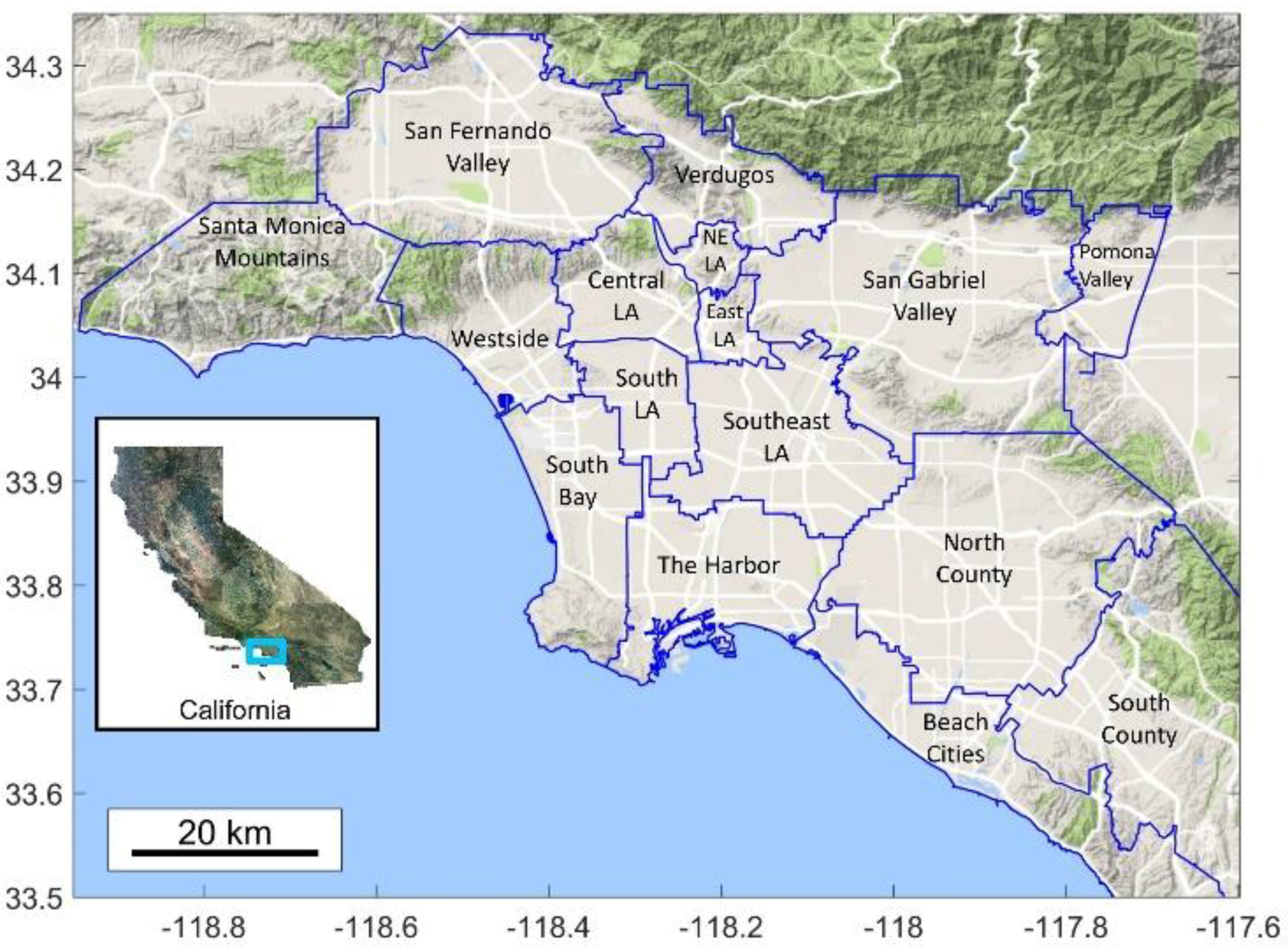
2.1. Study Region
2.2. Heat Vulnerability Index (HVI) Framework
2.2.1. Heat Exposure (E) Variables
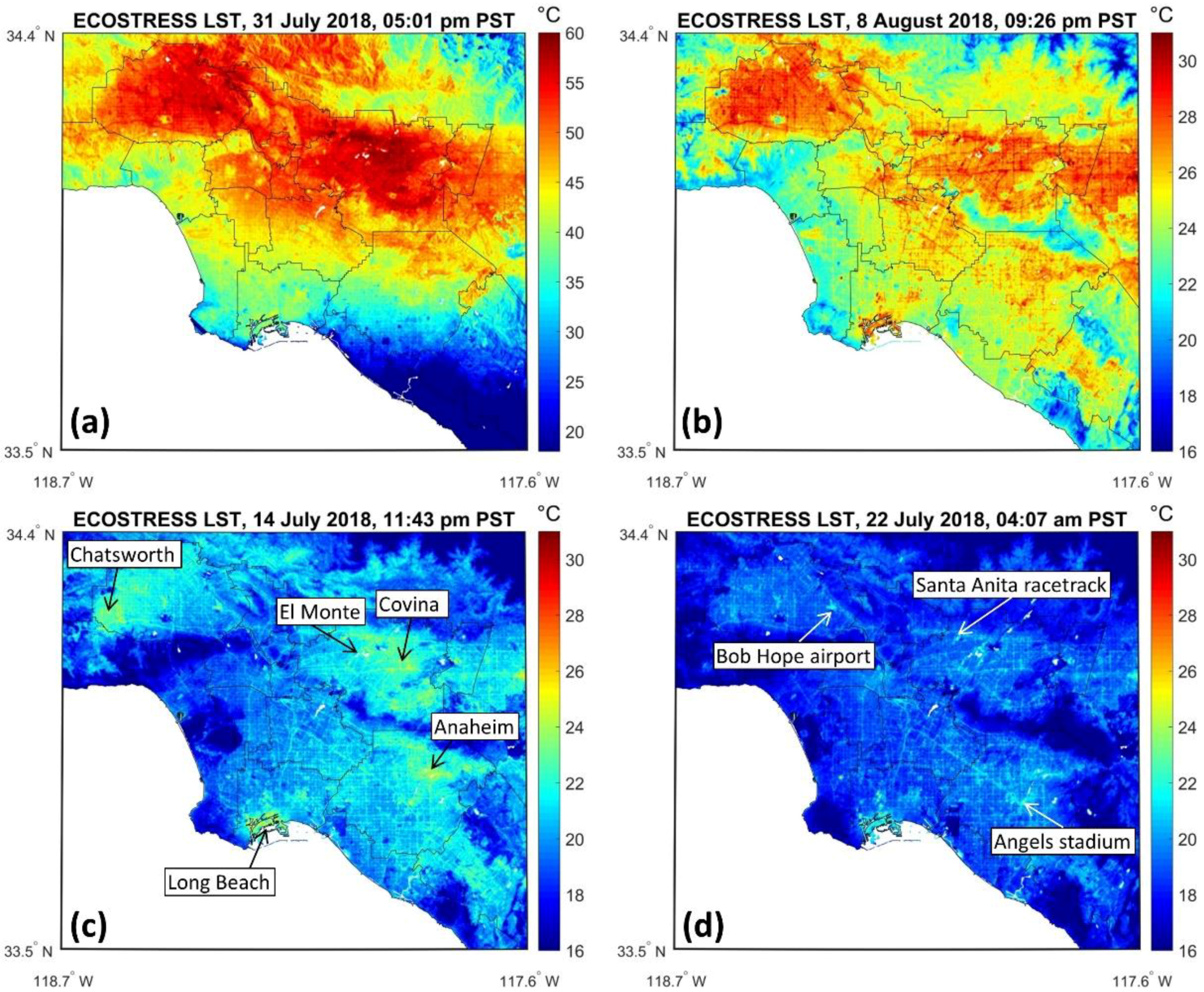
ECOSTRESS Land Surface Temperature
MODIS Land Surface Temperature
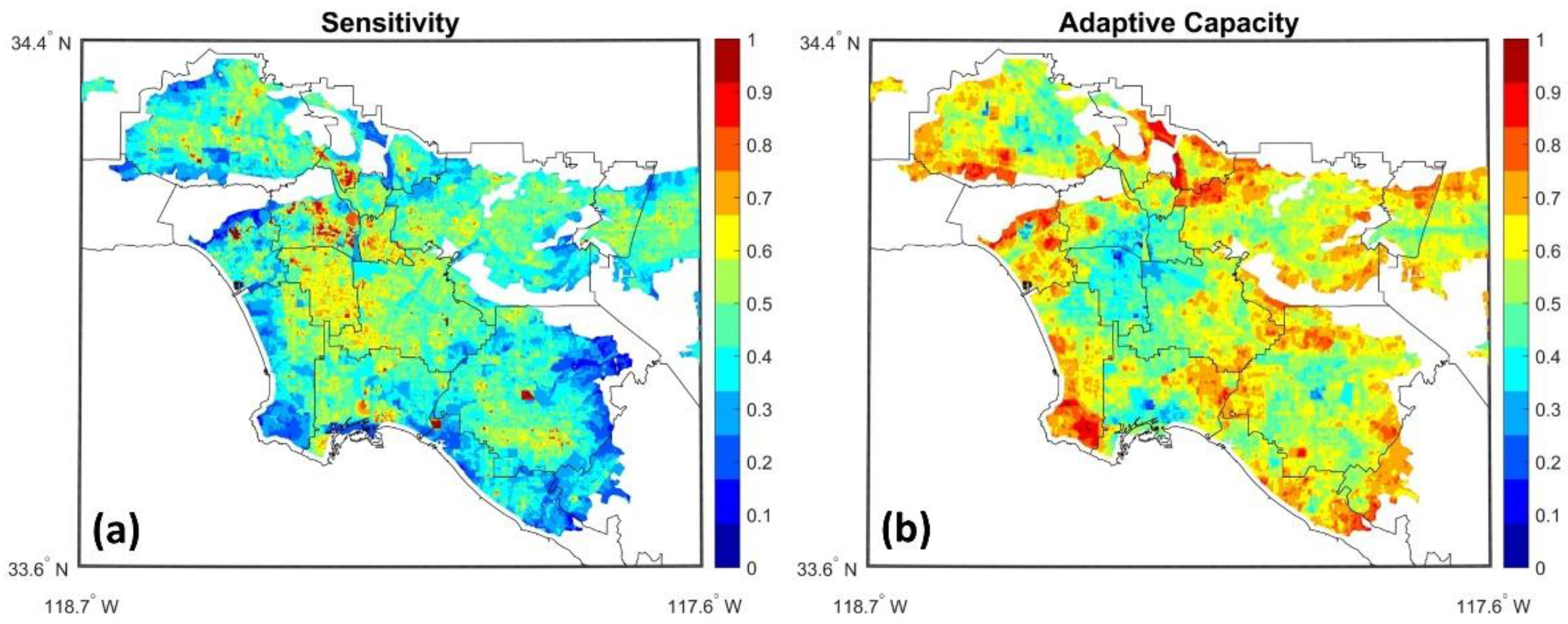
2.2.2. Sensitivity Variables
Elderly Population
Population Density
Poverty Level
Disabled Population
Unemployment
Building Height
2.2.3. Adaptive Capacity Variables
Education
Income
Green Vegetation Fraction
Distance to Cooling Centers
2.2.4. Principal Component Analysis
3. Results and Discussion
3.1. Statistical Analyses of Sensitivity and Adaptive Capacity Variables
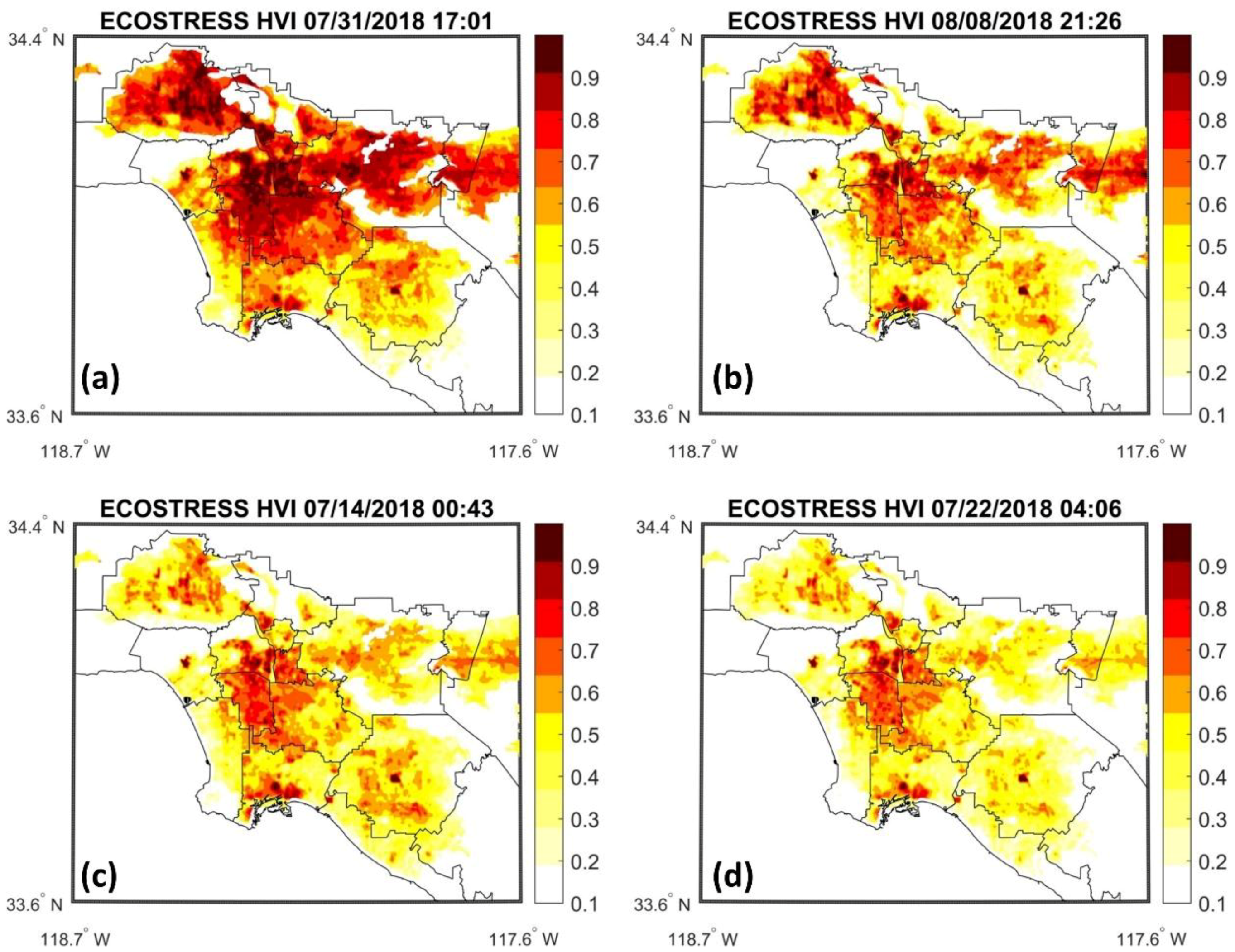
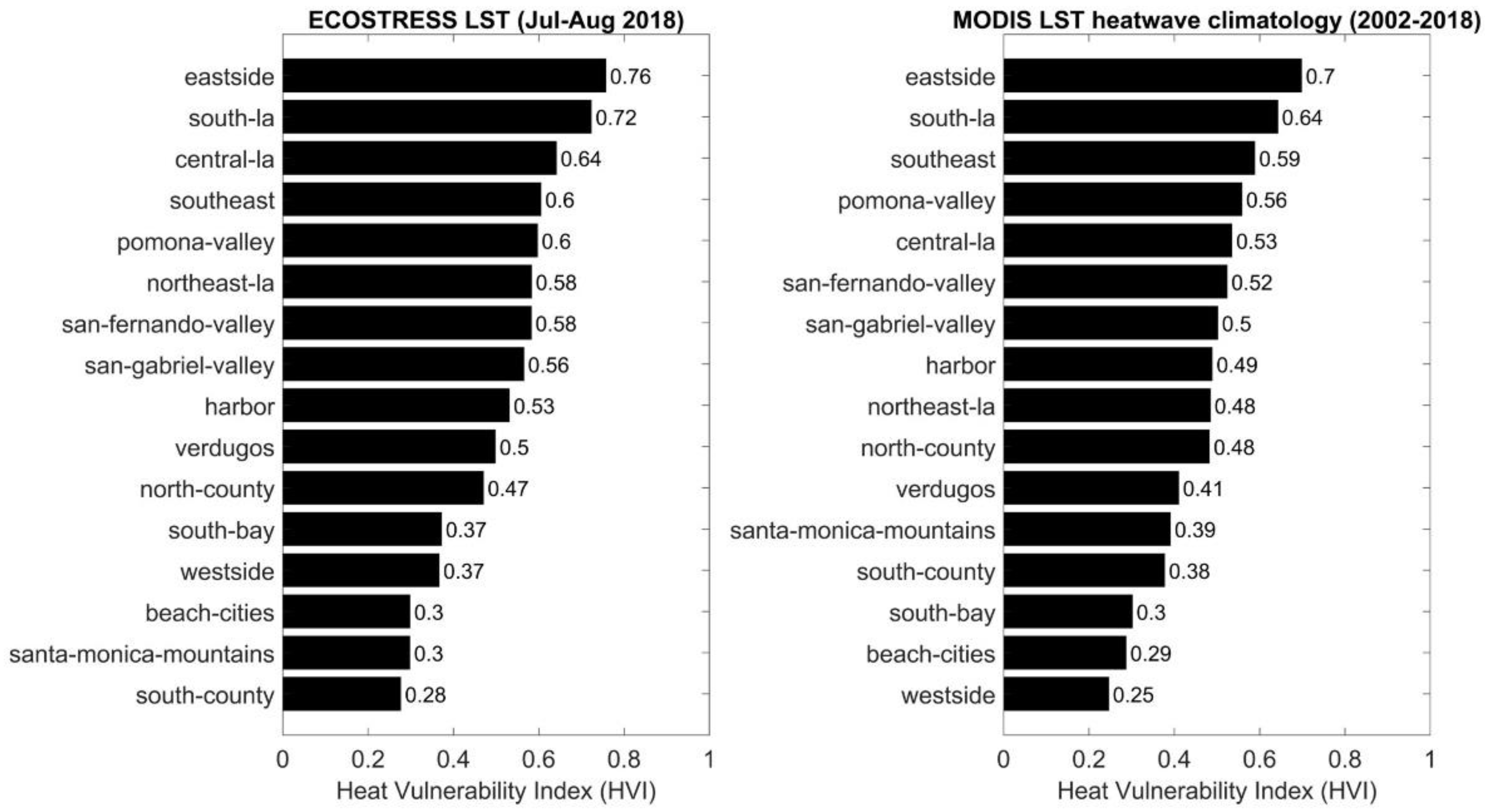
3.2. HVI from ECOSTRESS over the Diurnal Cycle
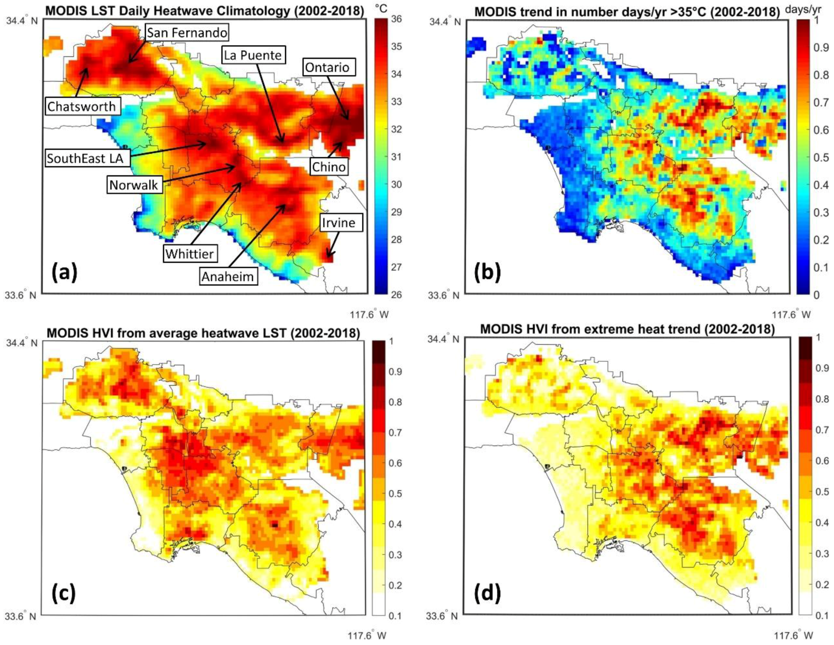
3.3. Historical HVI from MODIS Heatwave Climatology
4. Future Outlook and Validation Plans
5. Summary and Conclusions
Author Contributions
Funding
Acknowledgments
Conflicts of Interest
Appendix A

| Variable | Source | Temporal Scale | Spatial Scale | Index |
|---|---|---|---|---|
| Land Surface Temperature | ECOSTRESS | Diurnal cycle | 70 m | Exposure |
| Extreme Heat Trends | MODIS | 2002–2019 | 1 km | Exposure |
| Heatwave Average Daily Climatology | MODIS | 2002–2019 | 1 km | Exposure |
| Age of Housing | ACS | 2010 | 200 m | Sensitivity |
| Elderly Population | SEDAC | 2010 | 200 m | Sensitivity |
| Total Population | SEDAC | 2010 | 200 m | Sensitivity |
| Poverty | ACS | 2010 | 200 m | Sensitivity |
| Disabled Population | ACS | 2010 | 200 m | Sensitivity |
| Unemployment | ACS | 2010 | 200 m | Sensitivity |
| Building Height | University of Maryland | Static | 30 m | Sensitivity |
| Education | ACS | 2010 | 200 m | Adaptive Capacity |
| Income | ACS | 2010 | 200 m | Adaptive Capacity |
| Green Vegetation Fraction | AVIRIS | 2014 | 36 m | Adaptive Capacity |
| Normalized Difference Vegetation Index (NDVI) | Landsat | 16 days | 30 m | Adaptive Capacity |
| Variables | HVI | LST | Veg Fraction | Impervious Fraction | Building Height | Population Density | Poverty |
|---|---|---|---|---|---|---|---|
| HVI | 1 | ||||||
| LST | 0.69 | 1 | |||||
| Vegetation Fraction | −0.49 | −0.23 | 1 | ||||
| Impervious Fraction | 0.55 | 0.51 | −0.80 | 1 | |||
| Building Height | 0.51 | 0.17 | −0.64 | 0.74 | 1 | ||
| Population Density | 0.45 | 0.08 | −0.05 | 0.28 | 0.66 | 1 | |
| Poverty | 0.83 | 0.23 | −0.51 | 0.52 | 0.49 | 0.49 | 1 |
| Income | −0.85 | −0.30 | 0.61 | −0.61 | −0.56 | −0.45 | −0.96 |

References
- Perkins, S.E.; Alexander, L.V.; Nairn, J.R. Increasing frequency, intensity and duration of observed global heatwaves and warm spells. Geophys. Res. Lett. 2012, 39, L20714. [Google Scholar] [CrossRef]
- Anderson, G.B.; Bell, M.L. Heat Waves in the United States: Mortality Risk during Heat Waves and Effect Modification by Heat Wave Characteristics in 43 U.S. Communities. Environ. Health Persp. 2011, 119, 210–218. [Google Scholar] [CrossRef] [PubMed] [Green Version]
- Mora, C.; Dousset, B.; Caldwell, I.R.; Powell, F.E.; Geronimo, R.C.; Bielecki, C.R.; Counsell, C.W.W.; Dietrich, B.S.; Johnston, E.T.; Louis, L.V.; et al. Global risk of deadly heat. Nat. Clim. Chang. 2017, 7, 501–506. [Google Scholar] [CrossRef]
- United Nations, Department of Economic and Social Affairs, Population Division. World Population Prospects: The 2015 Revision, Key Findings and Advance Tables; Working paper no. Esa/p/wp.241; United Nations: New York, NY, USA, 2015. [Google Scholar]
- IPCC. The IPCC Fourth Assessment Report: Climate Change 2007: The Physical Science Basis; Cambridge University Press: Cambridge, UK, 2007; ISBN 978-0-521-88009-1. [Google Scholar]
- Akbari, H.; Pomerantz, M.; Taha, H. Cool surfaces and shade trees to reduce energy use and improve air quality in urban areas. Sol. Energy 2001, 70, 295–310. [Google Scholar] [CrossRef]
- Tan, J.G.; Zheng, Y.F.; Tang, X.; Guo, C.Y.; Li, L.P.; Song, G.X.; Zhen, X.R.; Yuan, D.; Kalkstein, A.J.; Li, F.R.; et al. The urban heat island and its impact on heat waves and human health in Shanghai. Int. J. Biometeorol. 2010, 54, 75–84. [Google Scholar] [CrossRef] [PubMed]
- Akbari, H. Shade trees reduce building energy use and CO2 emissions from power plants. Environ. Pollut. 2002, 116, S119–S126. [Google Scholar] [CrossRef]
- CDC. Climate Change and Extreme Heat Events 2013. Available online: http://www.cdc.gov/climateandhealth/pubs/ClimateChangeandExtremeHeatEvents.pdf (accessed on 12 september 2019).
- Gershunov, A.; Cayan, D.R.; Iacobellis, S.F. The Great 2006 Heat Wave over California and Nevada: Signal of an Increasing Trend. J. Clim. 2009, 22, 6181–6203. [Google Scholar] [CrossRef] [Green Version]
- Hulley, G.C.; Dousset, B.; Kahn, B. Compounding risk factors affecting heatwave severity in Southern California urban regions. Proc. Natl. Acad. Sci. USA 2019. in review. [Google Scholar]
- Bao, J.Z.; Li, X.D.; Yu, C.H. The Construction and Validation of the Heat Vulnerability Index, a Review. Int. J. Environ. Res. Pub. Health 2015, 12, 7220–7234. [Google Scholar] [CrossRef] [Green Version]
- Abson, D.J.; Dougill, A.J.; Stringer, L.C. Using Principal Component Analysis for information-rich socio-ecological vulnerability mapping in Southern Africa. Appl. Geogr. 2012, 35, 515–524. [Google Scholar] [CrossRef]
- Reid, C.E.; Mann, J.K.; Alfasso, R.; English, P.B.; King, G.C.; Lincoln, R.A.; Margolis, H.G.; Rubado, D.J.; Sabato, J.E.; West, N.L.; et al. Evaluation of a Heat Vulnerability Index on Abnormally Hot Days: An Environmental Public Health Tracking Study. Environ. Health Perspect. 2012, 120, 715–720. [Google Scholar] [CrossRef] [PubMed]
- Bradford, K.; Abrahams, L.S.; Hegglin, M.; Klima, K. A Heat Vulnerability Index and Adaptation Solutions for Pittsburgh, Pennsylvania. Environ. Sci. Technol. 2015, 49, 11303–11311. [Google Scholar] [CrossRef] [PubMed]
- Aubrecht, C.; Ozceylan, D. Identification of heat risk patterns in the U.S. National Capital Region by integrating heat stress and related vulnerability. Environ. Int. 2013, 56, 65–77. [Google Scholar] [CrossRef] [PubMed]
- Harlan, S.L.; Declet-Barreto, J.H.; Stefanov, W.L.; Petitti, D.B. Neighborhood Effects on Heat Deaths: Social and Environmental Predictors of Vulnerability in Maricopa County, Arizona. Environ. Health Persp. 2013, 121, 197–204. [Google Scholar] [CrossRef] [PubMed] [Green Version]
- Ho, H.C.; Knudby, A.; Huang, W. A Spatial Framework to Map Heat Health Risks at Multiple Scales. Int. J. Environ. Res. Public Health 2015, 12, 16110–16123. [Google Scholar] [CrossRef] [PubMed] [Green Version]
- Buscail, C.; Upegui, E.; Viel, J.-F. Mapping heatwave health risk at the community level for public health action. Int. J. Health Geogr. 2012, 11, 38. [Google Scholar] [CrossRef] [PubMed]
- Johnson, D.P.; Wilson, J.S.; Luber, G.C. Socioeconomic indicators of heat-related health risk supplemented with remotely sensed data. Int. J. Heal. Geogr. 2009, 8, 57. [Google Scholar] [CrossRef] [PubMed]
- Zhang, W.; McManus, P.; Duncan, E. A Raster-Based Subdividing Indicator to Map Urban Heat Vulnerability: A Case Study in Sydney, Australia. Int. J. Environ. Res. Public Health 2018, 15, 2516. [Google Scholar] [CrossRef] [PubMed]
- Mendez-Lazaro, P.; Muller-Karger, F.E.; Otis, D.; McCarthy, M.J.; Rodriguez, E. A heat vulnerability index to improve urban public health management in San Juan, Puerto Rico. Int. J. Biometeorol. 2018, 62, 709–722. [Google Scholar] [CrossRef] [PubMed]
- Räsänen, A.; Heikkinen, K.; Piila, N.; Juhola, S. Zoning and weighting in urban heat island vulnerability and risk mapping in Helsinki, Finland. Reg. Environ. Chang. 2019, 19, 1481–1493. [Google Scholar] [CrossRef] [Green Version]
- Wolf, T.; McGregor, G.; Analitis, A. Performance Assessment of a Heat Wave Vulnerability Index for Greater London, United Kingdom. Weather. Clim. Soc. 2014, 6, 32–46. [Google Scholar] [CrossRef] [Green Version]
- Tomlinson, C.J.; Chapman, L.; Thornes, J.E.; Baker, C.J. Including the urban heat island in spatial heat health risk assessment strategies: A case study for Birmingham, UK. Int. J. Health Geogr. 2011, 10, 42. [Google Scholar] [CrossRef] [PubMed]
- Morabito, M.; Crisci, A.; Gioli, B.; Gualtieri, G.; Toscano, P.; Di Stefano, V.; Orlandini, S.; Gensini, G.F. Urban-Hazard Risk Analysis: Mapping of Heat-Related Risks in the Elderly in Major Italian Cities. PLoS ONE 2015, 10, e0127277. [Google Scholar] [CrossRef] [PubMed]
- Chen, Q.; Ding, M.J.; Yang, X.C.; Hu, K.J.; Qi, J.G. Spatially explicit assessment of heat health risk by using multi-sensor remote sensing images and socioeconomic data in Yangtze River Delta, China. Int. J. Health Geogr. 2018, 17, 15. [Google Scholar] [CrossRef] [PubMed]
- Vescovi, L.; Rebetez, M.; Rong, F. Assessing public health risk due to extremely high temperature events: Climate and social parameters. Clim. Res. 2005, 30, 71–78. [Google Scholar] [CrossRef]
- Harlan, S.L.; Brazel, A.J.; Prashad, L.; Stefanov, W.L.; Larsen, L. Neighborhood microclimates and vulnerability to heat stress. Soc. Sci. Med. 2006, 63, 2847–2863. [Google Scholar] [CrossRef] [PubMed]
- Kershaw, S.E.; Millward, A.A. A spatio-temporal index for heat vulnerability assessment. Environ. Monit. Assess. 2012, 184, 7329–7342. [Google Scholar] [CrossRef]
- Hu, K.J.; Yang, X.C.; Zhong, J.M.; Fei, F.R.; Qi, J.G. Spatially Explicit Mapping of Heat Health Risk Utilizing Environmental and Socioeconomic Data. Environ. Sci. Technol. 2017, 51, 1498–1507. [Google Scholar] [CrossRef]
- Ho, H.C.; Knudby, A.; Walker, B.B.; Henderson, S.B. Delineation of Spatial Variability in the Temperature–Mortality Relationship on Extremely Hot Days in Greater Vancouver, Canada. Environ. Health Perspect. 2017, 125, 66–75. [Google Scholar] [CrossRef]
- MacIntyre, H.; Heaviside, C.; Taylor, J.; Picetti, R.; Symonds, P.; Cai, X.-M.; Vardoulakis, S. Assessing urban population vulnerability and environmental risks across an urban area during heatwaves–Implications for health protection. Sci. Total. Environ. 2018, 610, 678–690. [Google Scholar] [CrossRef]
- Dong, W.; Liu, Z.; Liao, H.; Tang, Q.; Li, X. New climate and socio-economic scenarios for assessing global human health challenges due to heat risk. Clim. Chang. 2015, 130, 505–518. [Google Scholar] [CrossRef] [Green Version]
- Krstic, N.; Yuchi, W.; Ho, H.C.; Walker, B.B.; Knudby, A.J.; Henderson, S.B. The Heat Exposure Integrated Deprivation Index (HEIDI): A data-driven approach to quantifying neighborhood risk during extreme hot weather. Environ. Int. 2017, 109, 42–52. [Google Scholar] [CrossRef] [PubMed]
- Sun, F.; Walton, D.B.; Hall, A. A Hybrid Dynamical–Statistical Downscaling Technique. Part II: End-of-Century Warming Projections Predict a New Climate State in the Los Angeles Region. J. Clim. 2015, 28, 4618–4636. [Google Scholar] [CrossRef]
- Wetherley, E.B.; McFadden, J.P.; Roberts, D.A. Megacity-scale analysis of urban vegetation temperatures. Remote. Sens. Environ. 2018, 213, 18–33. [Google Scholar] [CrossRef]
- Sobrino, J.A.; Oltra-Carrió, R.; Jiménez-Muñoz, J.C.; Julien, Y.; Soria, G.; Franch, B.; Mattar, C. Emissivity mapping over urban areas using a classification-based approach: Application to the Dual-use European Security IR Experiment (DESIREX). Int. J. Appl. Earth Obs. Geoinf. 2012, 18, 141–147. [Google Scholar] [CrossRef]
- Oyler, J.W.; Dobrowski, S.Z.; Holden, Z.A.; Running, S.W. Remotely Sensed Land Skin Temperature as a Spatial Predictor of Air Temperature across the Conterminous United States. J. Appl. Meteorol. Clim. 2016, 55, 1441–1457. [Google Scholar] [CrossRef]
- Good, E.J. An in situ-based analysis of the relationship between land surface “skin” and screen-level air temperatures. J. Geophys. Res. Atmos. 2016, 121, 8801–8819. [Google Scholar] [CrossRef]
- Hulley, G.C.; Ghent, D. Taking the Temperature of the Earth: Steps towards Integrated Understanding of Variability and Change, 1st ed.; Elsevier: Amsterdam, The Netherlands, 2019; p. 256. [Google Scholar]
- Voogt, J.A.; Oke, T.R. Complete Urban Surface Temperatures. J. Appl. Meteorol. 1997, 36, 1117–1132. [Google Scholar] [CrossRef]
- Voogt, J.A.; Oke, T.R. Effects of urban surface geometry on remotely-sensed surface temperature. Int. J. Remote Sens. 1998, 19, 895–920. [Google Scholar] [CrossRef]
- Voogt, J.A.; Oke, T.R. Radiometric Temperatures of Urban Canyon Walls obtained from Vehicle Traverses. Theor. Appl. Clim. 1998, 60, 199–217. [Google Scholar] [CrossRef]
- Arnfield, A.J. Two decades of urban climate research: A review of turbulence, exchanges of energy and water, and the urban heat island. Int. J. Clim. 2003, 23, 1–26. [Google Scholar] [CrossRef]
- Mildrexler, D.J.; Zhao, M.; Running, S.W. A global comparison between station air temperatures and MODIS land surface temperatures reveals the cooling role of forests. J. Geophys. Res. Biogeosci. 2011, 116. [Google Scholar] [CrossRef]
- Oyler, J.W.; Ballantyne, A.; Jencso, K.; Sweet, M.; Running, S.W. Creating a topoclimatic daily air temperature dataset for the conterminous United States using homogenized station data and remotely sensed land skin temperature. Int. J. Climatol. 2015, 35, 2258–2279. [Google Scholar] [CrossRef]
- Benali, A.; Carvalho, A.C.; Nunes, J.P.; Carvalhais, N.; Santos, A. Estimating air surface temperature in Portugal using MODIS LST data. Remote Sens. Environ. 2012, 124, 108–121. [Google Scholar] [CrossRef]
- Kloog, I.; Nordio, F.; Coull, B.A.; Schwartz, J. Predicting spatiotemporal mean air temperature using MODIS satellite surface temperature measurements across the Northeastern USA. Remote Sens. Environ. 2014, 150, 132–139. [Google Scholar] [CrossRef]
- Famiglietti, C.A.; Fisher, J.B.; Halverson, G.; Borbas, E.E. Global Validation of MODIS Near-Surface Air and Dew Point Temperatures. Geophys. Res. Lett. 2018, 45, 7772–7780. [Google Scholar] [CrossRef] [Green Version]
- Marzban, F.; Conrad, T.; Marzban, P.; Sodoudi, S. Estimation of the Near-Surface Air Temperature during the Day and Nighttime from MODIS in Berlin, Germany. Int. J. Adv. Remote Sens. GIS 2018, 7, 2478–2517. [Google Scholar] [CrossRef]
- Pichierri, M.; Bonafoni, S.; Biondi, R. Satellite air temperature estimation for monitoring the canopy layer heat island of Milan. Remote Sens. Environ. 2012, 127, 130–138. [Google Scholar] [CrossRef]
- Hu, L.; Brunsell, N.A. A new perspective to assess the urban heat island through remotely sensed atmospheric profiles. Remote Sens. Environ. 2015, 158, 393–406. [Google Scholar] [CrossRef]
- Vahmani, P.; Ban-Weiss, G.A.; Ban-Weiss, G. Impact of remotely sensed albedo and vegetation fraction on simulation of urban climate in WRF-urban canopy model: A case study of the urban heat island in Los Angeles. J. Geophys. Res. Atmos. 2016, 121, 1511–1531. [Google Scholar] [CrossRef]
- Wan, Z. New refinements and validation of the MODIS Land-Surface Temperature/Emissivity products. Remote Sens. Environ. 2008, 112, 59–74. [Google Scholar] [CrossRef]
- Hulley, G.C.; Hook, S.J. Intercomparison of versions 4, 4.1 and 5 of the MODIS Land Surface Temperature and Emissivity products and validation with laboratory measurements of sand samples from the Namib desert, Namibia. Remote Sens. Environ. 2009, 113, 1313–1318. [Google Scholar] [CrossRef]
- Islam, T.; Hulley, G.C.; Malakar, N.K.; Radocinski, R.G.; Guillevic, P.C.; Hook, S.J. A Physics-Based Algorithm for the Simultaneous Retrieval of Land Surface Temperature and Emissivity from VIIRS Thermal Infrared Data. IEEE Trans. Geosci. Remote Sens. 2017, 55, 563–576. [Google Scholar] [CrossRef]
- Hulley, G.C.; Hook, S.J. Generating Consistent Land Surface Temperature and Emissivity Products Between ASTER and MODIS Data for Earth Science Research. IEEE Trans. Geosci. Remote Sens. 2011, 49, 1304–1315. [Google Scholar] [CrossRef]
- Malakar, N.K.; Hulley, G.C.; Hook, S.J.; Laraby, K.; Cook, M.; Schott, J.R. An Operational Land Surface Temperature Product for Landsat Thermal Data: Methodology and Validation. IEEE Trans. Geosci. Remote Sens. 2018, 56, 5717–5735. [Google Scholar] [CrossRef]
- Hulley, G.; Malakar, N.; Islam, T.; Freepartner, R. NASA’s MODIS and VIIRS Land Surface Temperature and Emissivity Products: A Consistent and High Quality Earth System Data Record. IEEE Trans. Geosci. Remote Sens. 2017, 11, 522–535. [Google Scholar]
- Malakar, N.K.; Hulley, G.C. A water vapor scaling model for improved land surface temperature and emissivity separation of MODIS thermal infrared data. Remote Sens. Environ. 2016, 182, 252–264. [Google Scholar] [CrossRef]
- Oltra-Carrió, R.; Sobrino, J.A.; Franch, B.; Nerry, F. Land surface emissivity retrieval from airborne sensor over urban areas. Remote Sens. Environ. 2012, 123, 298–305. [Google Scholar] [CrossRef]
- Sobrino, J.A.; Oltra-Carrió, R.; Soria, G.; Bianchi, R.; Paganini, M. Impact of spatial resolution and satellite overpass time on evaluation of the surface urban heat island effects. Remote Sens. Environ. 2012, 117, 50–56. [Google Scholar] [CrossRef]
- Vanos, J.K.; Middel, A.; McKercher, G.R.; Kuras, E.R.; Ruddell, B.L. Hot playgrounds and children’s health: A multiscale analysis of surface temperatures in Arizona, USA. Landsc. Urban Plan. 2016, 146, 29–42. [Google Scholar] [CrossRef]
- Jenerette, G.D.; Harlan, S.L.; Stefanov, W.L.; Martin, C.A. Ecosystem services and urban heat riskscape moderation: Water, green spaces, and social inequality in Phoenix, USA. Ecol. Appl. 2011, 21, 2637–2651. [Google Scholar] [CrossRef] [PubMed]
- Dominguez, A.; Kleissl, J.; Luvall, J.C.; Rickman, D.L. High-resolution urban thermal sharpener (HUTS). Remote Sens. Environ. 2011, 115, 1772–1780. [Google Scholar] [CrossRef] [Green Version]
- Inamdar, A.K.; French, A.; Hook, S.; Vaughan, G.; Luckett, W. Land surface temperature retrieval at high spatial and temporal resolutions over the southwestern United States. J. Geophys. Res. Atmos. 2008, 113, 113. [Google Scholar] [CrossRef]
- Roberts, D.A.; Quattrochi, D.A.; Hulley, G.C.; Hook, S.J.; Green, R.O. Synergies between VSWIR and TIR data for the urban environment: An evaluation of the potential for the Hyperspectral Infrared Imager (HyspIRI) Decadal Survey mission. Remote Sens. Environ. 2012, 117, 83–101. [Google Scholar] [CrossRef]
- Sismanidis, P.; Keramitsoglou, I.; Kiranoudis, C.T.; Bechtel, B. Assessing the Capability of a Downscaled Urban Land Surface Temperature Time Series to Reproduce the Spatiotemporal Features of the Original Data. Remote Sens. 2016, 8, 274. [Google Scholar] [CrossRef]
- Bechtel, B.; Zaksek, K.; Hoshyaripour, G. Downscaling Land Surface Temperature in an Urban Area: A Case Study for Hamburg, Germany. Remote Sens. 2012, 4, 3184–3200. [Google Scholar] [CrossRef] [Green Version]
- Wang, Q.; Shi, W.; Atkinson, P.M.; Zhao, Y. Downscaling MODIS images with area-to-point regression kriging. Remote Sens. Environ. 2015, 166, 191–204. [Google Scholar] [CrossRef]
- Granero-Belinchon, C.; Michel, A.; Lagouarde, J.-P.; Sobrino, J.A.; Briottet, X. Multi-Resolution Study of Thermal Unmixing Techniques over Madrid Urban Area: Case Study of TRISHNA Mission. Remote Sens. 2019, 11, 1251. [Google Scholar] [CrossRef]
- Gillespie, A.; Rokugawa, S.; Matsunaga, T.; Cothern, J.; Hook, S.; Kahle, A. A temperature and emissivity separation algorithm for Advanced Spaceborne Thermal Emission and Reflection Radiometer (ASTER) images. IEEE Trans. Geosci. Remote Sens. 1998, 36, 1113–1126. [Google Scholar] [CrossRef]
- McGeehin, M.A.; Mirabelli, M. The Potential Impacts of Climate Variability and Change on Temperature-Related Morbidity and Mortality in the United States. Environ. Health Perspect. 2001, 109, 185. [Google Scholar]
- Oke, T. The urban energy balance. Prog. Phys. Geogr. Earth Environ. 1988, 12, 471–508. [Google Scholar] [CrossRef]
- Grimmond, C.S.B.; Oke, T.R. Heat Storage in Urban Areas: Local-Scale Observations and Evaluation of a Simple Model. J. Appl. Meteorol. 1999, 38, 922–940. [Google Scholar] [CrossRef]
- Kjelgren, R.; Montague, T. Urban tree transpiration over turf and asphalt surfaces. Atmos. Environ. 1998, 32, 35–41. [Google Scholar] [CrossRef]
- Akbari, H.; Matthews, H.D. Global cooling updates: Reflective roofs and pavements. Energy Build. 2012, 55, 2–6. [Google Scholar] [CrossRef]
- Akbari, H.; Menon, S.; Rosenfeld, A. Global cooling: Increasing world-wide urban albedos to offset CO2. Clim. Chang. 2009, 94, 275–286. [Google Scholar] [CrossRef]
- Oke, T.R. The energetic basis of the urban heat island. Q. J. R. Meteorol. Soc. 1982, 108, 1–24. [Google Scholar] [CrossRef]
- Hämmerle, M.; Gál, T.; Unger, J.; Matzarakis, A. Comparison of models calculating the sky view factor used for urban climate investigations. Theor. Appl. Clim. 2011, 105, 521–527. [Google Scholar] [CrossRef]
- Bureau, U.S.C. American Community Survey 1-year estimates. In Census Reporter Profile Page; Los Angeles, CA, USA, 2017; Available online: https://censusreporter.org/profiles/16000US0644000-los-angeles-ca/ (accessed on 12 September 2019).
- Gershunov, A.; Guirguis, K. California heat waves in the present and future. Geophys. Res. Lett. 2012, 39, 18. [Google Scholar] [CrossRef]
- Clemesha, R.E.S.; Guirguis, K.; Gershunov, A.; Small, I.J.; Tardy, A. California heat waves: Their spatial evolution, variation, and coastal modulation by low clouds. Clim. Dyn. 2018, 50, 4285–4301. [Google Scholar] [CrossRef]
- Wilhelmi, O.V.; Hayden, M.H. Connecting people and place: A new framework for reducing urban vulnerability to extreme heat. Environ. Res. Lett. 2010, 5, 014021. [Google Scholar] [CrossRef]
- Inostroza, L.; Palme, M.; De La Barrera, F. A Heat Vulnerability Index: Spatial Patterns of Exposure, Sensitivity and Adaptive Capacity for Santiago de Chile. PLoS ONE 2016, 11, e0162464. [Google Scholar] [CrossRef] [PubMed]
- Cutter, S.L.; Boruff, B.J.; Shirley, W.L. Social Vulnerability to Environmental Hazards. Soc. Sci. Q. 2003, 84, 242–261. [Google Scholar] [CrossRef]
- Bulkeley, H.; Tuts, R. Understanding urban vulnerability, adaptation and resilience in the context of climate change. Local Environ. 2013, 18, 646–662. [Google Scholar] [CrossRef] [Green Version]
- Turner, B.L.; Kasperson, R.E.; Matson, P.A.; McCarthy, J.J.; Corell, R.W.; Christensen, L.; Eckley, N.; Kasperson, J.X.; Luers, A.; Martello, M.L.; et al. A framework for vulnerability analysis in sustainability science. Proc. Natl. Acad. Sci. USA 2003, 100, 8074–8079. [Google Scholar] [CrossRef] [PubMed] [Green Version]
- Klinenberg, E. Heat Wave: A Social Autopsy of Disaster in Chicago; University of Chicago Press: Chicago, IL, USA, 2002. [Google Scholar]
- Leichenko, R.M.; Solecki, W.D. Consumption, Inequity, and Environmental Justice: The Making of New Metropolitan Landscapes in Developing Countries. Soc. Nat. Resour. 2008, 21, 611–624. [Google Scholar] [CrossRef]
- Hayden, M.H.; Wilhelmi, O.V.; Banerjee, D.; Greasby, T.; Cavanaugh, J.L.; Nepal, V.; Boehnert, J.; Sain, S.; Burghardt, C.; Gower, S. Adaptive Capacity to Extreme Heat: Results from a Household Survey in Houston, Texas. Weather Clim. Soc. 2017, 9, 787–799. [Google Scholar] [CrossRef]
- Hayden, M.H.; Brenkert-Smith, H.; Wilhelmi, O.V. Differential Adaptive Capacity to Extreme Heat: A Phoenix, Arizona, Case Study. Weather Clim. Soc. 2011, 3, 269–280. [Google Scholar] [CrossRef]
- Hulley, G.C.; Dousset, B. Climatology and rising trends of extreme heat over Los Angeles observed from NASA MODIS land surface temperature data (MYD21). Remote Sens. Environ. 2019. in review. [Google Scholar]
- ECO2LSTEv001. ECOSTRESS Land Surface Temperature and Emissivity Daily L2 Global 70 m. Available online: Https://lpdaac.Usgs.Gov/products/eco2lstev001/ (accessed on 12 September 2019).
- Herold, M.; Roberts, D. Spectral characteristics of asphalt road aging and deterioration: Implications for remote-sensing applications. Appl. Opt. 2005, 44, 4327–4334. [Google Scholar] [CrossRef]
- Justice, C.; Townshend, J. Special issue on the moderate resolution imaging spectroradiometer (MODIS): A new generation of land surface monitoring. Remote Sens. Environ. 2002, 83, 1–2. [Google Scholar] [CrossRef]
- Wan, Z.M. New refinements and validation of the collection-6 MODIS land-surface temperature/emissivity product. Remote Sens. Environ. 2014, 140, 36–45. [Google Scholar] [CrossRef]
- Perkins, S.E.; Alexander, L.V. On the Measurement of Heat Waves. J. Clim. 2013, 26, 4500–4517. [Google Scholar] [CrossRef]
- Nairn, J.R.; Fawcett, R.J.B. The Excess Heat Factor: A Metric for Heatwave Intensity and Its Use in Classifying Heatwave Severity. Int. J. Environ. Res. Public Health 2015, 12, 227–253. [Google Scholar] [CrossRef] [PubMed]
- Socioeconomic Data and Applications Center (SEDAC). Available online: https://sedac.ciesin.columbia.edu/ (accessed on 12 September 2019).
- Seirup, L.; Yetman, G. U.S. Census Grids (Summary File 3), 2000: Metropolitan Statistical Areas; NASA Socioeconomic Data and Applications Center (SEDAC): Palisades, NY, USA, 2006; Available online: https://0-doi-org.brum.beds.ac.uk/10.7927/H4Z31WJ0 (accessed on 4 August 2018).
- Whitman, S.; Good, G.; Donoghue, E.R.; Benbow, N.; Shou, W.; Mou, S. Mortality in Chicago attributed to the July 1995 heat wave. Am. J. Public Health 1997, 87, 1515–1518. [Google Scholar] [CrossRef] [PubMed]
- Conti, S.; Meli, P.; Minelli, G.; Solimini, R.; Toccaceli, V.; Vichi, M.; Beltrano, C.; Perini, L. Epidemiologic study of mortality during the Summer 2003 heat wave in Italy. Environ. Res. 2005, 98, 390–399. [Google Scholar] [CrossRef] [PubMed]
- Fouillet, A.; Rey, G.; Laurent, F.; Pavillon, G.; Bellec, S.; Ghihenneuc-Jouyaux, C.; Clavel, J.; Jougla, E.; Hémon, D. Excess mortality related to the August 2003 heat wave in France. Int. Arch. Occup. Environ. Health 2006, 80, 16–24. [Google Scholar] [CrossRef] [Green Version]
- Knowlton, K.; Rotkin-Ellman, M.; King, G.; Margolis, H.G.; Smith, D.; Solomon, G.; Trent, R.; English, P. The 2006 California Heat Wave: Impacts on Hospitalizations and Emergency Department Visits. Environ. Health Persp. 2009, 117, 61–67. [Google Scholar] [CrossRef] [PubMed]
- Semenza, J. Excess hospital admissions during the July 1995 heat wave in Chicago. Am. J. Prev. Med. 1999, 16, 269–277. [Google Scholar] [CrossRef]
- Bouchama, A.; Dehbi, M.; Mohamed, G.; Matthies, F.; Shoukri, M.; Menne, B. Prognostic Factors in Heat Wave–Related DeathsA Meta-analysis. Arch. Intern. Med. 2007, 167, 2170. [Google Scholar] [CrossRef]
- Stone, B.; Hess, J.J.; Frumkin, H. Urban Form and Extreme Heat Events: Are Sprawling Cities More Vulnerable to Climate Change Than Compact Cities? Environ. Health Perspect. 2010, 118, 1425–1428. [Google Scholar] [CrossRef] [Green Version]
- Borrell, C.; Marí-Dell’Olmo, M.; Rodríguez-Sanz, M.; Garcia-Olalla, P.; Caylà, J.A.; Benach, J.; Muntaner, C. Socioeconomic position and excess mortality during the heat wave of 2003 in Barcelona. Eur. J. Epidemiol. 2006, 21, 633–640. [Google Scholar] [CrossRef] [PubMed]
- Jones, T.S. Morbidity and mortality associated with the July 1980 heat wave in St Louis and Kansas City, Mo. JAMA 1982, 247, 3327–3331. [Google Scholar] [CrossRef] [PubMed]
- Yardley, J.; Sigal, R.J.; Kenny, G.P. Heat health planning: The importance of social and community factors. Glob. Environ. Chang. 2011, 21, 670–679. [Google Scholar] [CrossRef]
- Chestnut, L.G.; Breffle, W.S.; Smith, J.B.; Kalkstein, L.S. Analysis of differences in hot-weather-related mortality across 44 U.S. metropolitan areas. Environ. Sci. Policy 1998, 1, 59–70. [Google Scholar] [CrossRef]
- Naughton, M. Heat-related mortality during a 1999 heat wave in Chicago. Am. J. Prev. Med. 2002, 22, 221–227. [Google Scholar] [CrossRef]
- Heiner, K.S.; Strug, L.; Patz, J.A.; Curriero, F.C.; Samet, J.M.; Zeger, S.L. Temperature and Mortality in 11 Cities of the Eastern United States. Am. J. Epidemiol. 2002, 155, 80–87. [Google Scholar]
- Kim, Y.; Joh, S. A vulnerability study of the low-income elderly in the context of high temperature and mortality in Seoul, Korea. Sci. Total. Environ. 2006, 371, 82–88. [Google Scholar] [CrossRef] [PubMed]
- Patz, J.A.; McGeehin, M.A.; Bernard, S.M.; Ebi, K.L.; Epstein, P.R.; Grambsch, A.; Gubler, D.J.; Reiter, P.; Romieu, I.; Rose, J.B.; et al. The Potential Health Impacts of Climate Variability and Change for the United States: Executive Summary of the Report of the Health Sector of the U.S. National Assessment. Environ. Health Perspect. 2000, 108, 367–376. [Google Scholar] [CrossRef] [PubMed]
- Belmin, J.; Golmard, J.L. Mortality related to the heatwave in 2003 in France: Forcasted or over the top. Presse Med. 2005, 34, 627–628. [Google Scholar] [CrossRef]
- Semenza, J.C.; Rubin, C.H.; Falter, K.H.; Selanikio, J.D.; Wilhelm, J.L.; Flanders, W.D.; Howe, H.L. Heat-Related Deaths during the July 1995 Heat Wave in Chicago. N. Engl. J. Med. 1996, 335, 84–90. [Google Scholar] [CrossRef] [PubMed]
- Bernard, S.M.; McGeehin, M.A. Municipal Heat Wave Response Plans. Am. J. Public Health 2004, 94, 1520–1522. [Google Scholar] [CrossRef] [PubMed]
- Gallie, D.; Paugam, S.; Jacobs, S. unemployment, poverty and social isolation: Is there a vicious circle of social exclusion? Eur. Soc. 2003, 5, 1–32. [Google Scholar] [CrossRef]
- Voogt, J.; Oke, T. Thermal remote sensing of urban climates. Remote Sens. Environ. 2003, 86, 370–384. [Google Scholar] [CrossRef]
- Wang, P.; Huang, C.; Tilton, J.C. Mapping Three-dimensional Urban Structure by Fusing Landsat and Global Elevation Data. arXiv 2018, arXiv:1807.04368. [Google Scholar]
- O’Neill, M.S.; Zanobetti, A.; Schwartz, J. Modifiers of the temperature and mortality association in seven US cities. Am. J. Epidemiol. 2003, 157, 1074–1082. [Google Scholar] [CrossRef] [PubMed]
- Knowlton, K.; Lynn, B.; Goldberg, R.A.; Rosenzweig, C.; Hogrefe, C.; Rosenthal, J.K.; Kinney, P.L. Projecting Heat-Related Mortality Impacts Under a Changing Climate in the New York City Region. Am. J. Public Health 2007, 97, 2028–2034. [Google Scholar] [CrossRef]
- Johnson, D.P.; Stanforth, A.; Lulla, V.; Luber, G. Developing an applied extreme heat vulnerability index utilizing socioeconomic and environmental data. Appl. Geogr. 2012, 35, 23–31. [Google Scholar] [CrossRef]
- Johnson, D.P.; Wilson, J.S. The socio-spatial dynamics of extreme urban heat events: The case of heat-related deaths in Philadelphia. Appl. Geogr. 2009, 29, 419–434. [Google Scholar] [CrossRef]
- Roberts, D.; Gardner, M.; Church, R.; Ustin, S.; Scheer, G.; Green, R. Mapping Chaparral in the Santa Monica Mountains Using Multiple Endmember Spectral Mixture Models. Remote Sens. Environ. 1998, 65, 267–279. [Google Scholar] [CrossRef]
- Dwyer, J.; Roy, D.; Sauer, B.; Jenkerson, C.; Zhang, H.; Lymburner, L. Analysis Ready Data: Enabling Analysis of the Landsat Archive. Remote Sens. 2018, 10, 1363. [Google Scholar] [CrossRef]
- Tucker, C.J.; Newcomb, W.W.; Los, S.O.; Prince, S.D. Mean and inter-year variation of growing-season normalized difference vegetation index for the Sahel 1981–1989. Int. J. Remote Sens. 1991, 12, 1133–1135. [Google Scholar] [CrossRef]
- Geerken, R.; Zaitchik, B.; Evans, J.P. Classifying rangeland vegetation type and coverage from NDVI time series using Fourier Filtered Cycle Similarity. Int. J. Remote Sens. 2005, 26, 5535–5554. [Google Scholar] [CrossRef]
- Telesca, L.; Lasaponara, R. Quantifying intra-annual persistent behaviour in SPOT-VEGETATION NDVI data for Mediterranean ecosystems of southern Italy. Remote Sens. Environ. 2006, 101, 95–103. [Google Scholar] [CrossRef]
- Wardlow, B.; Egbert, S.; Kastens, J. Analysis of time-series MODIS 250 m vegetation index data for crop classification in the U.S. Central Great Plains. Remote Sens. Environ. 2007, 108, 290–310. [Google Scholar] [CrossRef] [Green Version]
- Kovats, R.S.; Kristie, L.E. Heatwaves and public health in Europe. Eur. J. Public Health 2006, 16, 592–599. [Google Scholar] [CrossRef] [PubMed] [Green Version]
- ArcGIS Hub. Available online: Https://hub.Arcgis.Com/datasets/ (accessed on 12 September 2019).
- Abdi, H.; Williams, L.J. Principal component analysis. Wiley Interdiscip. Rev. Comput. Stat. 2010, 2, 433–459. [Google Scholar] [CrossRef]
- Jolliffe, I.T. Graphical Representation of Data Using Principal Components; Springer Inc.: New York, NY, USA, 2002. [Google Scholar]
- Carlson, T.N.; Ripley, D.A. On the relation between NDVI, fractional vegetation cover, and leaf area index. Remote Sens. Environ. 1997, 62, 241–252. [Google Scholar] [CrossRef]
- Dousset, B.; Gourmelon, F.; Laaidi, K.; Zeghnoun, A.; Giraudet, E.; Bretin, P.; Mauri, E.; Vandentorren, S. Satellite monitoring of summer heat waves in the Paris metropolitan area. Int. J. Climatol. 2011, 31, 313–323. [Google Scholar] [CrossRef]
- Hajat, S.; Kovats, R.; Atkinson, R.W.; Haines, A. Impact of hot temperatures on death in London: A time series approach. J. Epidemiol. Community Health 2002, 56, 367–372. [Google Scholar] [CrossRef]
- Laaidi, K.; Zeghnoun, A.; Dousset, B.; Bretin, P.; Vandentorren, S.; Giraudet, E.; Beaudeau, P. The Impact of Heat Islands on Mortality in Paris during the August 2003 Heat Wave. Environ. Health Persp. 2012, 120, 254–259. [Google Scholar] [CrossRef] [Green Version]
- Stewart, I.D.; Oke, T.R. Local Climate Zones for Urban Temperature Studies. Bull. Am. Meteorol. Soc. 2012, 93, 1879–1900. [Google Scholar] [CrossRef]
- Chuang, W.-C.; Gober, P. Predicting Hospitalization for Heat-Related Illness at the Census-Tract Level: Accuracy of a Generic Heat Vulnerability Index in Phoenix, Arizona (USA). Environ. Health Perspect. 2015, 123, 606–612. [Google Scholar] [CrossRef] [PubMed]
- Maier, G.; Grundstein, A.; Jang, W.; Li, C.; Naeher, L.P.; Shepherd, M. Assessing the Performance of a Vulnerability Index during Oppressive Heat across Georgia, United States. Weather Clim. Soc. 2014, 6, 253–263. [Google Scholar] [CrossRef]
- Luber, G.; McGeehin, M. Climate Change and Extreme Heat Events. Am. J. Prev. Med. 2008, 35, 429–435. [Google Scholar] [CrossRef] [PubMed]
- OSHPD. Patient Discharge Data (PDD) Dictionary. Available online: https://oshpd.ca.gov/ml/v1/resources/document?rs:path=/Data-And-Reports/Documents/Request/Data-Documentation/DataDictionary_PDD_2018_Nonpublic.pdf (accessed on 12 September 2019).
- OSHPD. Emergency Department (ED) and Ambulatory Surgery (AS) Data Dictionary. Available online: https://oshpd.ca.gov/ml/v1/resources/document?rs:path=/Data-And-Reports/Documents/Request/Data-Documentation/DataDictionary_EDAS_2018_Nonpublic.pdf (accessed on 12 September 2019).
- Katsouyanni, K.; Pantazopoulou, A.; Touloumi, G.; Tselepidaki, I.; Moustris, K.P.; Asimakopoulos, D.; Poulopoulou, G.; Trichopoulos, D. Evidence for Interaction between Air Pollution and High Temperature in the Causation of Excess Mortality. Arch. Environ. Health Int. J. 1993, 48, 235–242. [Google Scholar] [CrossRef]
- Taha, H.; Konopacki, S.; Akbari, H. Impacts of Lowered Urban Air Temperatures on Precursor Emission and Ozone Air Quality. J. Air Waste Manag. Assoc. 1998, 48, 860–865. [Google Scholar] [CrossRef] [PubMed]
- Goldsmith, J.R. Three Los Angeles heat waves. In Environmental Epidemiology: Epidemiologic Investigation of Community Environmental Health Problems; CRC Press: Boca Raton, FL, USA, 2019; p. 73. [Google Scholar]
- Patel, D.; Jian, L.; Xiao, J.G.; Jansz, J.; Yun, G.; Robertson, A. Joint effect of heatwaves and air quality on emergency department attendances for vulnerable population in Perth, Western Australia, 2006 to 2015. Environ. Res. 2019, 174, 80–87. [Google Scholar] [CrossRef] [PubMed]


| PC1 | PC2 | PC3 | PC4 | ||
|---|---|---|---|---|---|
| Adaptability 1 “Socioeconomic status” | Green vegetation fraction | 0.42 | −0.05 | 0.13 | −0.02 |
| Income | 0.50 | −0.06 | −0.05 | −0.01 | |
| Education | 0.47 | 0.09 | −0.11 | −0.07 | |
| Sensitivity 1 “Congestion” | Elderly | 0.11 | 0.62 | 0.03 | −0.15 |
| Population density | −0.11 | 0.57 | −0.08 | −0.03 | |
| Building height | −0.12 | 0.42 | −0.04 | 0.24 | |
| Sensitivity 2 “Isolation” | Poverty | −0.36 | 0.12 | 0.21 | −0.04 |
| Disabled | 0.01 | −0.08 | 0.67 | −0.07 | |
| Unemployment | −0.23 | −0.07 | 0.48 | −0.05 | |
| Adaptability 2 | Cooling center proximity | −0.11 | −0.11 | −0.16 | 0.82 |
| Vulnerability Ranking | HVI (%) (mean ± SD) | Number of Cooling Centers | Green Space (%) | Temperature (°C) (mean ± SD) |
|---|---|---|---|---|
| 1. East LA | 76 ± 8 | 0 | 14 | 29.0 ± 0.8 |
| 2. South LA | 72 ± 10 | 3 | 15 | 26.8 ± 1.0 |
| 3. Central LA | 64 ± 19 | 1 | 18 | 27.4 ± 1.5 |
| 4. Southeast LA | 61 ± 10 | 13 | 18 | 27.5 ± 1.2 |
| 5. Pomona Valley | 59 ± 14 | 9 | 24 | 28.8 ± 1.7 |
| 6. Northeast LA | 58 ± 10 | 3 | 25 | 28.6 ± 1.1 |
| 7. San Fernando | 58 ± 15 | 5 | 26 | 29.6 ± 1.5 |
| 8. San Gabriel | 56 ± 12 | 13 | 26 | 29.4 ± 2.0 |
| 9. Harbor | 53 ± 14 | 11 | 18 | 25.2 ± 1.5 |
| 10. Verdugos | 50 ± 19 | 4 | 32 | 29.0 ± 1.4 |
| 11. North County | 47 ± 12 | 1 | 25 | 25.5 ± 2.1 |
| 12. South Bay | 37 ± 18 | 3 | 23 | 23.9 ± 1.5 |
| 13. Westside | 36 ± 17 | 2 | 30 | 24.6 ± 1.3 |
| 14. Beach cities | 30 ± 12 | 0 | 25 | 17.6 ± 3.5 |
| 15. Santa Monica | 30 ± 6 | 0 | 39 | 25.1 ± 1.6 |
| 16. South County | 27 ± 9 | 0 | 27 | 20.5 ± 2.9 |
© 2019 by the authors. Licensee MDPI, Basel, Switzerland. This article is an open access article distributed under the terms and conditions of the Creative Commons Attribution (CC BY) license (http://creativecommons.org/licenses/by/4.0/).
Share and Cite
Hulley, G.; Shivers, S.; Wetherley, E.; Cudd, R. New ECOSTRESS and MODIS Land Surface Temperature Data Reveal Fine-Scale Heat Vulnerability in Cities: A Case Study for Los Angeles County, California. Remote Sens. 2019, 11, 2136. https://0-doi-org.brum.beds.ac.uk/10.3390/rs11182136
Hulley G, Shivers S, Wetherley E, Cudd R. New ECOSTRESS and MODIS Land Surface Temperature Data Reveal Fine-Scale Heat Vulnerability in Cities: A Case Study for Los Angeles County, California. Remote Sensing. 2019; 11(18):2136. https://0-doi-org.brum.beds.ac.uk/10.3390/rs11182136
Chicago/Turabian StyleHulley, Glynn, Sarah Shivers, Erin Wetherley, and Robert Cudd. 2019. "New ECOSTRESS and MODIS Land Surface Temperature Data Reveal Fine-Scale Heat Vulnerability in Cities: A Case Study for Los Angeles County, California" Remote Sensing 11, no. 18: 2136. https://0-doi-org.brum.beds.ac.uk/10.3390/rs11182136