Multisensor Characterization of Urban Morphology and Network Structure

Lamont Doherty Earth Observatory, Columbia University, Palisades, NY 10964, USA
Remote Sens. 2019, 11(18), 2162; https://0-doi-org.brum.beds.ac.uk/10.3390/rs11182162
Submission received: 14 July 2019
/
Revised: 7 September 2019
/
Accepted: 9 September 2019
/
Published: 17 September 2019
(This article belongs to the Special Issue Remote Sensing for Urban Morphology)
Abstract
:The combination of decameter resolution Sentinel 2 and hectometer resolution VIIRS offers the potential to quantify urban morphology at scales spanning the range from individual objects to global scale settlement networks. Multi-season spectral characteristics of built environments provide an independent complement to night light brightness compared for 12 urban systems. High fractions of spectrally stable impervious surface combined with persistent deep shadow between buildings are compared to road network density and outdoor lighting inferred from night light. These comparisons show better spatial agreement and more detailed representation of a wide range of built environments than possible using Landsat and DMSP-OLS. However, they also show that no single low luminance brightness threshold provides optimal spatial correlation to built extent derived from Sentinel in different urban systems. A 4-threshold comparison of 6 regional night light networks shows consistent spatial scaling, spanning 3 to 5 orders of magnitude in size and number with rank-size slopes consistently near −1. This scaling suggests a dynamic balance among the processes of nucleation, growth and interconnection. Rank-shape distributions based on √Area/Perimeter of network components scale similarly to rank-size distributions at higher brightness thresholds, but show both progressive then abrupt increases in fractal dimension of the largest, most interconnected network components at lower thresholds.

1. Introduction
The spatial form of urban land cover informs our understanding of its function and evolution. The diversity of the myriad forms of human settlement worldwide suggests that any general understanding of urban morphology requires a systematic characterization of this diversity in both space and time. To establish causal relationships between form and function, the characterization must span the range of scales from the individual objects (e.g., streets, buildings, open spaces) to individual settlements. As the spatial scale of consideration expands from individual settlements to collections of settlements, the range of factors influencing the larger scale morphology must expand accordingly.
Remote sensing provides synoptic perspectives on urban morphology and evolution over the past 40+ years. These perspectives are invaluable for understanding the form of modern urban environments and their evolving relationship to the environments that host them. The utility of remote sensing to rigorous characterization of urban morphology was recognized by Mesev and Longley [1], who introduced a methodology to quantify the fractal form of urban morphology from remotely sensed optical imagery in the context of location theory. This provided a basis for establishing the utility of remotely sensed imagery to rigorous quantitative analysis of the built environment in conjunction with the theoretical basis for its fractal nature as observed at comparable scales [2]. However, since this time, the vast majority of effort in the area of urban remote sensing has focused on the challenges of identification and classification of settlements, with less attention being given to the quantification of the built environment’s form and its relationship to the function of urban systems.
Despite the unique benefits offered by remote sensing, there are also challenges that complicate most attempts to use it for mapping of urban land cover (see [3] for an overview). Most significant is the dual challenge of definition and recognition. The diversity of definitions of urban [4] poses a challenge because many do not have direct analogs in physically measurable quantities—particularly from space. In addition, the task of recognition is complicated by the diversity of physical form of settlements worldwide. The compositional heterogeneity of materials found in built environments violates the cardinal assumption of spectral homogeneity on which almost all thematic classification schemes are based [5,6]. Nonetheless, the potential gains in terms of retrospective global mapping and operational monitoring are so great that considerable effort is still devoted to developing improved approaches to mapping built environments using remote sensing (see [7] for a recent review).
The combination of decameter resolution Sentinel 2 and hectometer resolution VIIRS (Visible Infrared Imaging Radiometer Suite) offers the potential to quantify the relationship between urban morphology and scaling at scales spanning the range from individual objects to global scale settlement networks. City size distributions have been a topic of considerable interest to economists, geographers, and urbanists since the discovery of a consistent scaling relationship among cities on the basis of population by Auerbach in 1913 [8]. Despite a widely observed inconsistency of scaling when defined on the basis of population [9], analysis of city size distributions defined on the basis of area derived from night light observations has shown more consistent agreement at regional, continental and global scales [10], leading to the recognition that these distributions can be treated as spatial networks. This conceptualization confers the benefit that existing, more general, theory of network scaling can be extended to bounded spatial networks such as those resulting from land cover [11]. One objective of this analysis is to explore the relationship between urban morphology and area scaling of networks of lighted development. In order to establish the relationship between night light and land cover, a comparison of Sentinel 2 spectral properties and VIIRS night light is conducted over a set of intercomparison sites, each containing a major city and surrounding land cover network.
The approach used in this study will apply two methodologies in parallel; a multi-season spectral unmixing methodology previously-developed for Landsat to newly available Sentinel 2 and a progressive thresholding scaling methodology previously developed for DMSP-OLS (Defense Meteorological Satellite Program–Operational Line Scanner) night light to VIIRS annual composites recently released by Elvidge and colleagues [12,13]. The first part of this study will briefly discuss the use of multi-season optical imagery to distinguish built environments on the basis of spectrally stable impervious surfaces and persistent building shadow and will then compare a diversity of built environments worldwide using both Sentinel 2 reflectance and VIIRS dnb night light. Having established the relationship between multitemporal reflectance and night light brightness, the second part of the study will compare the relationship between urban morphology, area scaling and spatial network structure of a variety of spectrally stable built environments with VIIRS dnb night light observations.
2. Materials and Methods
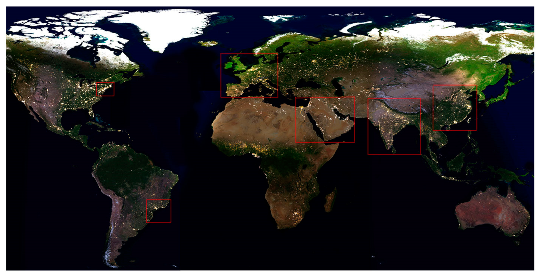
A set of 12 Sentinel 2 + VIIRS intercomparison sites was chosen on the basis of biome, level, and intensity of development, land cover diversity and cloud-free data availability. In addition to the intercomparison sites, a set of 6 regional study areas was chosen for VIIRS spatial network analysis. These larger study areas each include at least one intercomparison site but are chosen to encompass a full regional network of lighted urban development with boundaries generally based on observed geographic extents of night light. In two cases (USA and Brazil), spatial subsets of lighted development within larger networks are intentionally chosen to illustrate morphology of sub-networks. The regional study area extents are show in Figure 1.
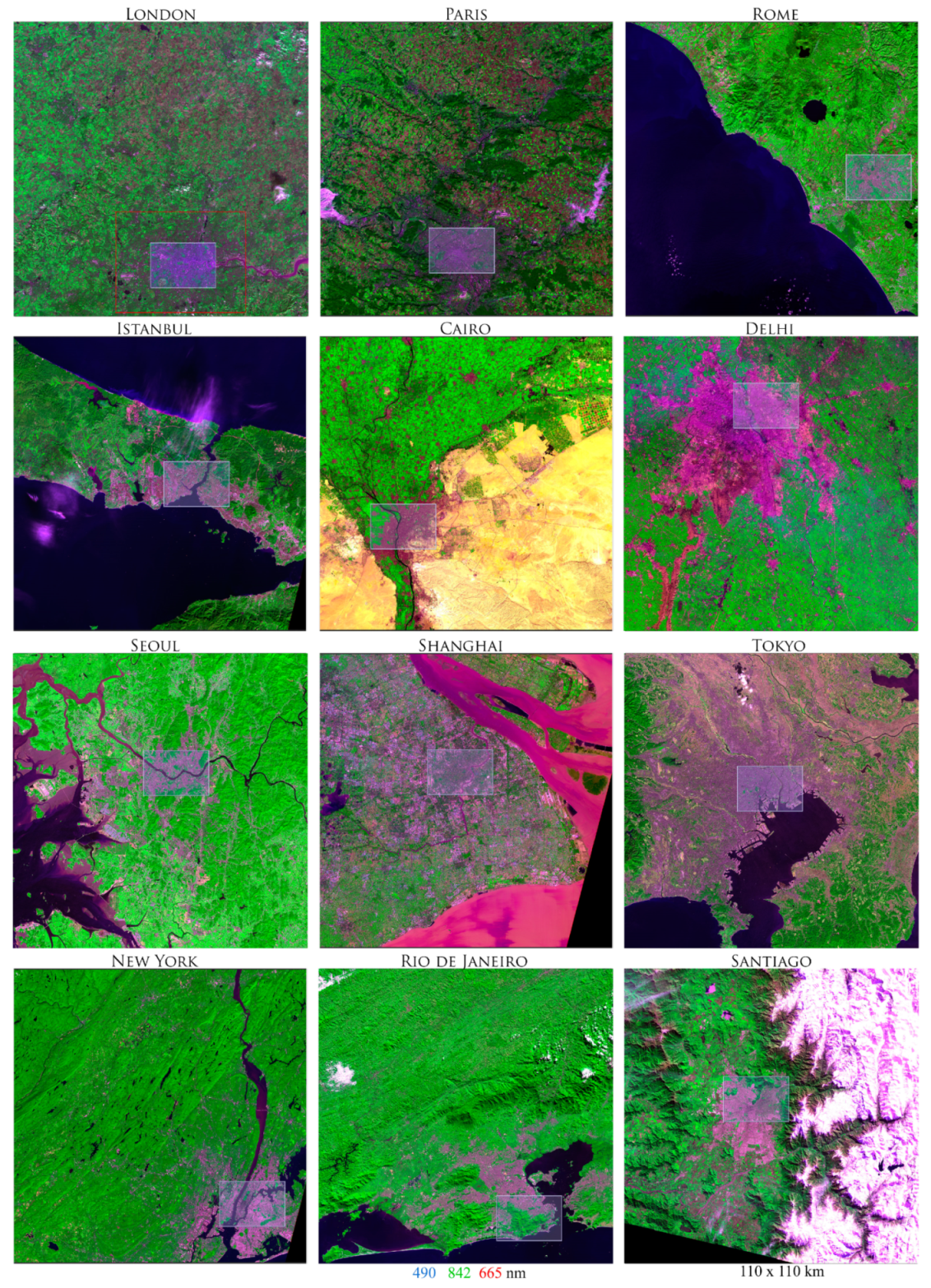
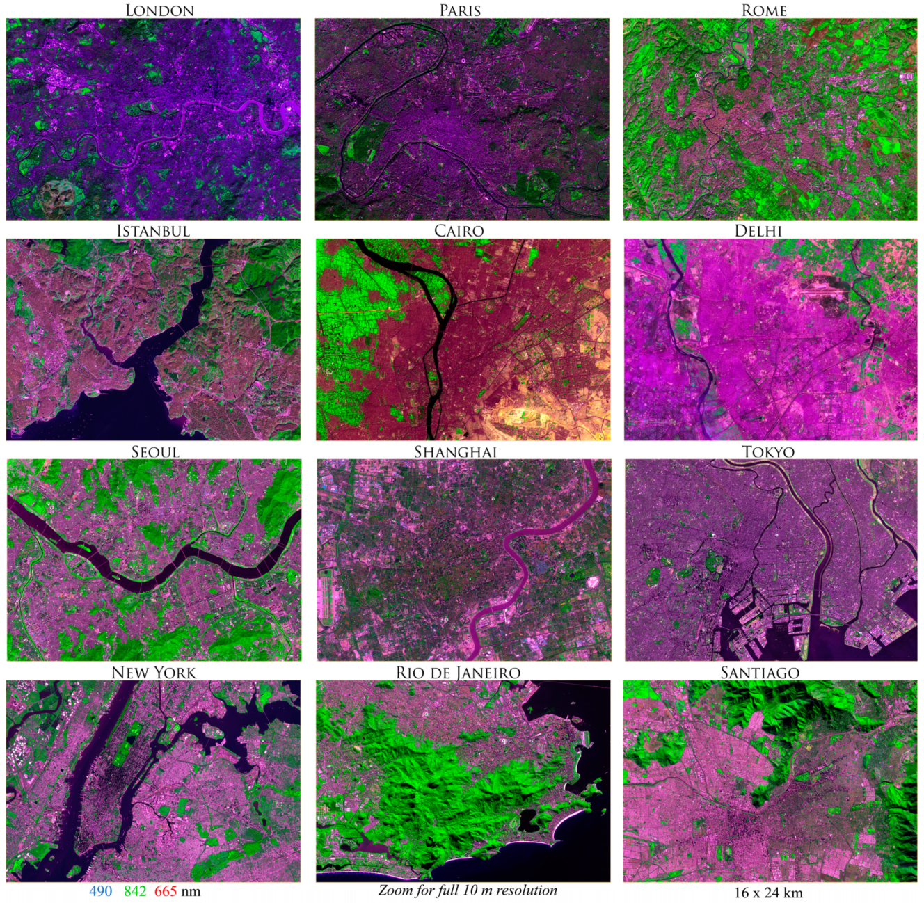
Intercomparison sites were chosen to include a major city as well as the full diversity of its land cover setting with multiple gradients of development intensity (Figure 2). Full resolution examples of each built up urban core (Figure 3) illustrate the benefit of using 10 m imagery for mapping urban land cover. Individual buildings and transportation thoroughfares are generally resolved, considerably reducing the ambiguity introduced by the spatial aliasing of Landsat’s 30 m IFOV. Sentinel 2 Top of Atmosphere (ToA) reflectance products were obtained from the USGS EDC via earthexplorer.usgs.gov. For each of 12 single-tile (110 × 110 km) intercomparison sites, three to five mostly or entirely cloud-free single tile acquisitions were selected for dates with contrasting solar illumination and vegetation phenology phase (Table 1). For cities spanning two tiles within the same swath (therefore date), two tiles were mosaicked and a 10,980 × 10,980 subset was used. In the case of the London site, persistent cloud cover precluded use of a full tile and limited the multi-season extents to a smaller subset in the sidelap of adjacent swaths (Figure 2). ToA reflectance images for the 11 VSWIR bands (omitting bands 9 and 10) were resampled to the 10 m resolution of the four VNIR bands and unmixed using a constrained linear spectral mixture model with standardized spectral endmembers (EMs) derived from 1.4 million Sentinel 2 spectra worldwide [14] The full set of standardized EMs includes: (1) rock and soil Substrate, (2) illuminated photosynthetic Vegetation, and (3) Dark surfaces like deep shadow and water, as well as (4) ice and snow, (5) evaporites, and (6) reefs and submerged substrates. As in previous analyses with 30 m Landsat and 2 m commercial multispectral sensors, a simple 3 EM model based on S, V and D EMs is able to represent aggregate land cover reflectances with <0.05 RMS misfit for >98% of spectra [15]. The generality of the global model is applicable in urban settings because of the spectral similarity of pervious and impervious substrates. A similarity that leads to the considerable challenge of mapping impervious surface based on spectral properties alone. Individual date SVD fraction maps were coregistered to compute multi-season mean (μ) and standard deviation (σ) maps for each SVD EM fraction at each intercomparison site.
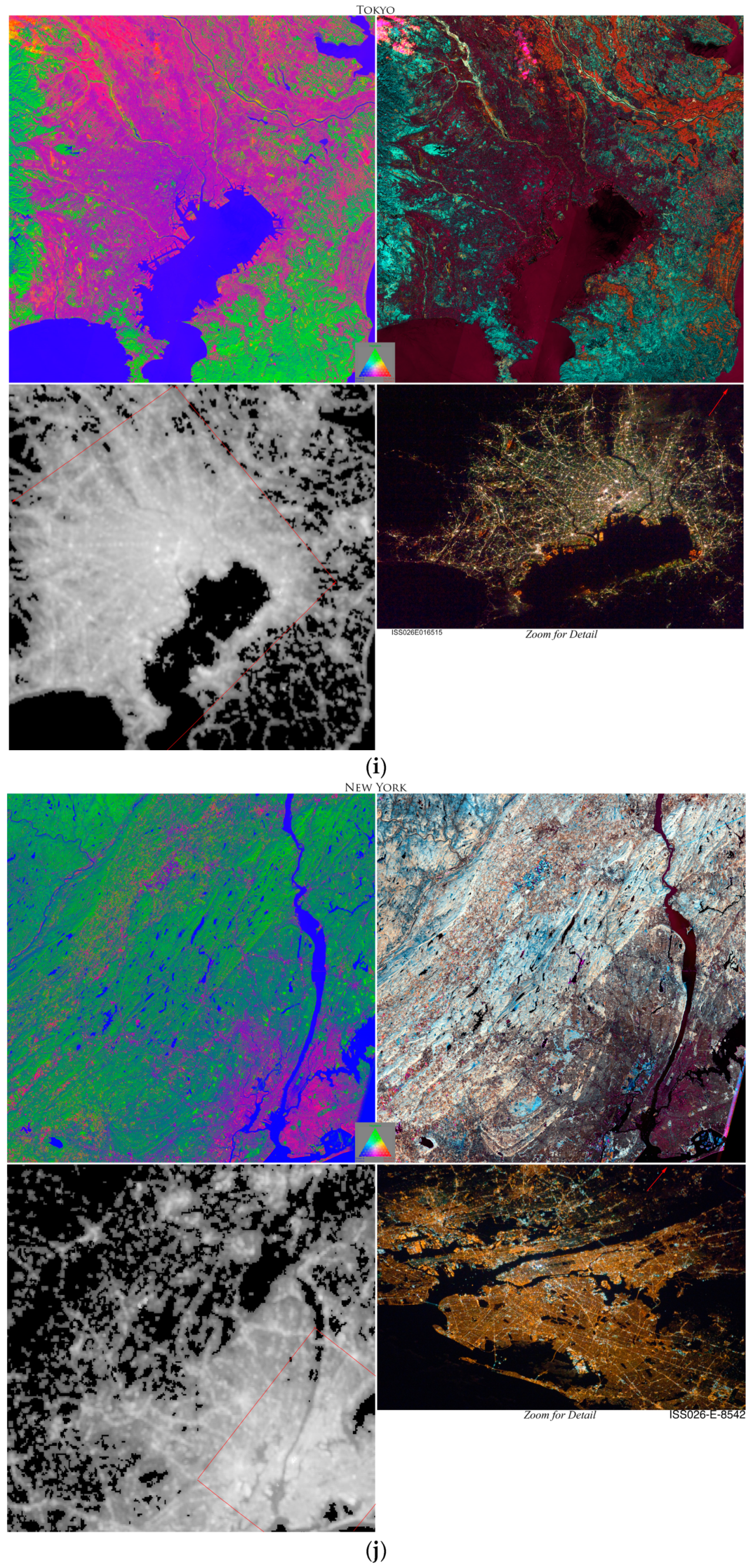
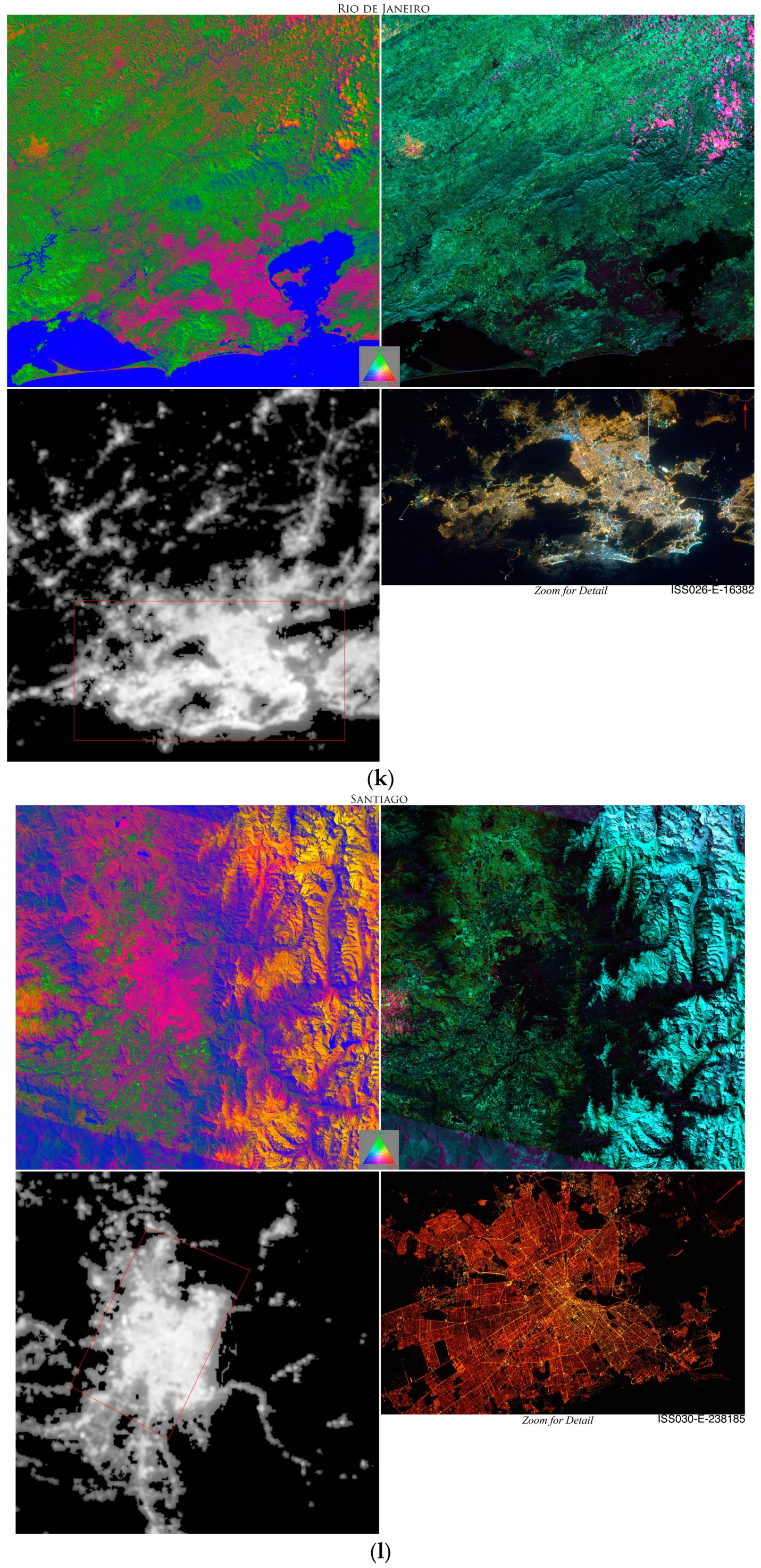
VIIRS dnb annual mean luminance composites for 2016 were obtained from https://www.ngdc.noaa.gov/eog/viirs/download_dnb_composites.html. In order to quantify the land cover diversity and seasonal variability within each 500 m VIIRS pixel, the VIIRS composite for each intercomparison site was reprojected into the UTM zone of the corresponding Sentinel 2 tile, and coregistered to the Sentinel 2 multi-season SVD composite. The VIIRS pixel value for each 10 m Sentinel pixel was extracted from the coregistered grid for correlation and heterogeneity analysis. Direct side by side comparisons of Log10 annual mean dnb luminance and SVD μ and σ composites are shown for each intercomparison site in Figure 4. In addition, astronaut photographs taken from the International Space station (circa 2013) are shown for comparison. The regional subsets used for the network analysis were reprojected from the native cylindrical projection to 500 m resolution equal area projections (Americas: Molleweide, Eurasia/Africa: Sinusoidal).
2.1. Multi-Season Spectral Characterization of Urban Land Cover
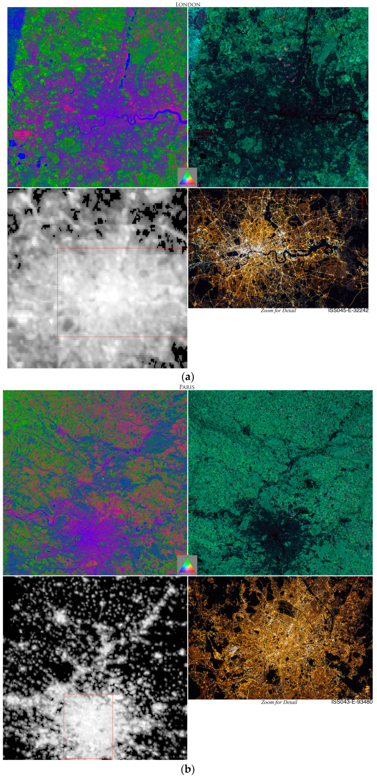
The Sentinel 2 SVD composites and VIIRS dnb composites in Figure 4 show a clear correspondence between brighter night light and lower seasonal variability (σ) in S, V, and D. The correspondence between night light brightness and seasonal mean (μ) is less consistent but generally corresponds to a range of mixtures of illuminated impervious substrate (S) and shadow (D). As discussed by [16,17,18], the relatively low seasonal variability is a result of three characteristics of most built environments; (1) Persistent shadow between buildings, (2) spectral stability of impervious surface relative to moisture-varying soils, and (3) relatively low abundance of vegetation. Accordingly, the seasonal mean SVD mixtures of these areas have relatively high D fractions (shadow), varying S fractions (impervious), and low V fractions.
The relationships between aggregate land cover and its seasonal variation in the SVD mixing space are related, in part, to the scale and compositional homogeneity of land cover within the pixel IFOV. At one extreme, pixels dominated by impervious surface tend to be spectrally stable, varying primarily with seasonal illumination if shadow area is comparable to illuminated area (e.g., buildings + streets). At the opposite extremes are pixels with large seasonal variations in either vegetation abundance or soil moisture. While the seasonal variability of compositionally (therefore spectrally) mixed pixels tends to vary with 3D relief and illumination, the seasonal variability of built up land cover tends to diminish with increasing shadow fraction resulting from greater building relief compared to illuminated nadir-facing surface area. This suggests that the fundamental properties of the SVD μ and σ spaces can be represented by the relationship between the magnitude of the SVD μ and σ vectors in these spaces.
The magnitude of the μ and σ vectors in SVD space are used here to represent the spectral homogeneity and multi-season spectral variability as:
Homogeneity = (μS2 + μV2 + μD2) 1/2
Variability = (σS2 + σV2 + σD2) 1/2
Homogeneity represents SVD mixtures as points in a mixing space—bounded by the plane representing the SVD fractions’ unit sum constraint. Because of this constraint, the largest homogeneity values are associated with pure pixels lying on or near one axis of the space. In contrast, the variability also represents an SVD space corresponding to the seasonal variability of each fraction in each pixel—but it is not subject to a unit sum constraint so the greatest variability can be associated with either pure or mixed pixels.
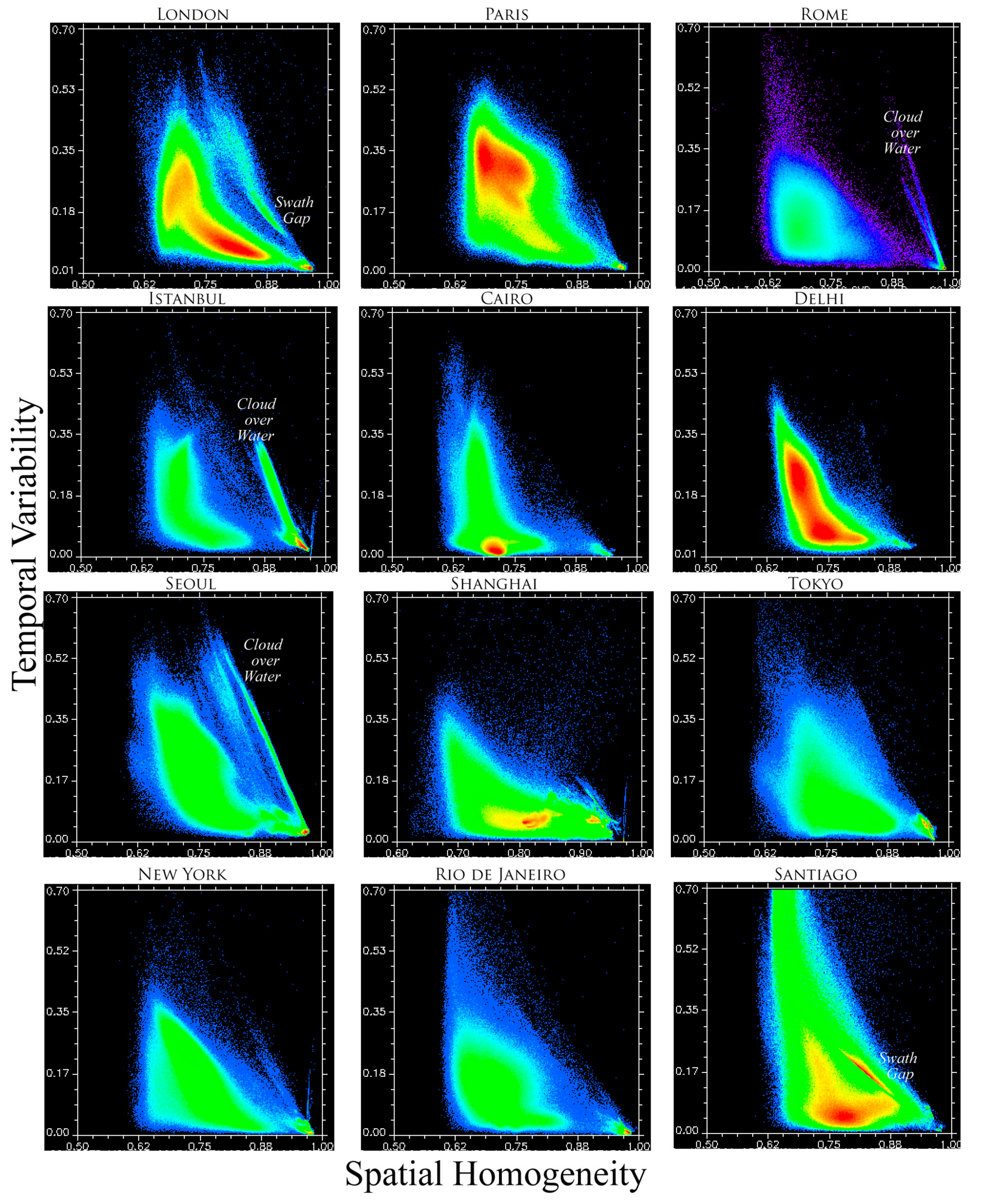
There is a consistent relationship between H and V for all 12 intercomparison site landscapes. Figure 5 shows full-tile scatterplots of spectral homogeneity versus variability for each of the 12 intercomparison sites. As expected, maximum seasonal variability diminishes with increasing spatial homogeneity at the pixel scale. It is noteworthy that these spaces are continuous—but with a prominent separation between spectrally stable water with maximum homogeneity and the somewhat less homogeneous shadow-dominated areas of urban cores with deep street canyons. The consistently inverse relationship suggests a single metric to incorporate the continuum of both of these spectrotemporal properties;
2.2. Network Identification by Progressive Segmentation
Spatial network structure of continuous fields, like night light brightness, can be quantified using progressive segmentation. Because the VIIRS dnb luminance composites are continuous fields, it is possible to impose multiple low luminance thresholds to create suites of binary maps of the spatial extent and size distribution of night light exceeding a progression of thresholds. Earlier analyses of DMSP-OLS night light [19] and comparisons in Figure 5 suggest no direct correspondence between a single brightness level and urban land cover so multiple thresholds are used to quantify the effects of progressive segmentation on the resulting distributions of lighted and non-lighted area. By progressively segmenting the continuous field into spatially contiguous areas above and below each threshold we create a series of illumination maps that can be used to quantify sensitivity of the resulting network structure to brightness threshold. Each continuous field of night light is projected into an equal area projection and segmented using the more conservative (smaller, less connected components) Rook’s case in which spatial contiguity is defined on the basis of 4 shared edges of each pixel. To account for spatial autocorrelation of the input imagery and avoid large numbers of spurious detections, a minimum segment size of 9 pixels is imposed. In two regions (W. Europe and S. Asia), a larger limit of 16 pixels is applied to eliminate large numbers very small detections at the lowest light threshold. A more detailed description of the progressive segmentation methodology is given by [10] and [11]. The progressive segmentation shows the changing spatial extent and structure of different ranges of luminance. For each low luminance threshold, the area and perimeter of each spatially contiguous segment is calculated to produce distinct area and perimeter distributions for each region and threshold.
2.3. Morphology Characterization by Area-Perimeter Distribution
A fundamental determinant of urban morphology is the fractal dimension of the built area [2]. While defined in terms of the scaling properties of a self-similar object, the fractal dimension of a city, or any spatially contiguous land cover, can be thought of as a measure of the complexity of its boundary or shape. A very smooth simple boundary (e.g., a circle) has a dimension of 1, but as the boundary becomes more complex, and self-similar across scales, the dimension of the boundary approaches 2 as it fills the space of the plane more completely. While a variety of methods have been developed to estimate fractal dimension from different spatial proxies for urban extent (See Batty and Longley (1996) for an extensive treatment), a relatively simple and commonly used metric is based on the area-perimeter relationship. In this analysis the area and perimeter distributions of the spatially contiguous segments that result from the low luminance thresholding are used to characterize the shapes of the segments—as well as the scaling properties of individual settlements and network components.
2.4. Network Characterization by Rank-Size and Rank-Shape Distribution
Spatial scaling of the spatial networks resulting from the thresholding is quantified using the rank-size distribution, in which the area of each spatially contiguous segment (i.e., lighted patch) is sorted by size to yield its ordinal rank, from largest to smallest. In the context of a spatial network, the size of each contiguous segment is analogous to the size of a single network component and the rank-size plot is analogous to the component size distribution [20]. Because the rank-size distributions of night light span several (4–6) orders of magnitude in both size and rank, they are displayed on log–log plots. Because these distributions generally form straight lines, power law exponents are estimated to quantify their slopes. While linear rank-size distributions are often assumed to be generated by power law processes, it may be difficult or even impossible to conclusively eliminate other long-tailed distributions (e.g., log–normal) from consideration. Hence the use of the power law here is merely a tool to quantify the linearity, slope and domain of the rank-size distributions used to infer the spatial scaling properties of the night light networks. To estimate the power law exponents, domain, uncertainty and validity, the approach given by [21] is used. This procedure repeatedly computes maximum likelihood estimates of the power law exponent for increasing subsets of the upper tail of the distribution and identifies a lower tail cutoff coinciding with the minimum of the Kolmogorov–Smirnov goodness-of-fit statistic. This cutoff gives an indication of the domain (range of spatial scales) over which the rank size distribution can be plausibly described with a power law.
3. Results
3.1. Consistency of Spectrotemporal Characteristics
The decrease in maximum temporal variability with spectral homogeneity is a consistent characteristic of all 12 intercomparison sites. In each case, the decrease in variability with increasing homogeneity is a combined result of the spectral stability of the impervious substrate and the persistence of deep shadow. However, there is considerable variability in this relationship among the different sites. This is evident from the variability of the scatterplots in Figure 5. This variability is presumably a result of differences in building material as well as scaling of building heights and spacings that determine the relative amounts of illumination and shadowing. This variability precludes using the homogeneity, variability and stability for quantitative comparisons among sites – even though they clearly correspond to the density of built surface over the gradient from urban core to periphery. These metrics are useful for direct comparison of the built area density to the night light brightness (e.g., Figure 6), and to demonstrate the site-specific threshold correlations (e.g., Figure 7) but without some form of cross calibration, the metrics are not valid for computation of morphology parameters. In addition, the presence of water bodies would require a masking procedure to prevent conflation of the two distributions.
3.2. VIIRS + Sentinel Comparisons
One of the primary complications of using night light composites to map built environments is the presence of “blooming” [22,23] or overglow [19]. These lower luminance halos surrounding bright light sources result from atmospheric scattering as well as upward diffuse scattering from reflective surfaces near the light source [24]. Comparisons between the Log10 VIIRS dnb annual mean luminance and the astronaut photographs shown in Figure 4 clearly depict the order of magnitude lower luminance “halos” surrounding bright sources. While the greater dynamic range and signal/noise of the VIIRS dnb sensor reduces overglow considerably, compared to the DMSP OLS sensor [25,26], it can still be seen clearly in areas where brightly lighted development is adjacent to water and in comparisons of the VIIRS dnb composites with the astronaut photos in Figure 4. The photos do not show overglow because the cameras used by the astronauts do not have the dynamic range or sensitivity of the VIIRS sensor to detect the low luminance halos. For the same reason, the photos do not capture the smaller dimmer light sources that VIIRS does. The effects of overglow can be reduced by imposing a low luminance threshold, but this results in attenuation of smaller, dimmer light sources unrelated to the overglow from bright sources and thereby much of the useful information content of the data [19].
Comparison of VIIRS dnb Log10 luminance distributions of the intercomparison sites reveal a characteristic multimodal distribution of brightness that is not apparent in large area distributions because of the large dynamic range and dominance of vast numbers of unlighted pixels. Multimodal luminance distributions are shown for the 12 intercomprison sites in Figure 6. In 9 of the 12 distributions multiple modes are clearly visible, while in the remaining 3 a second mode appears as an asymmetric shoulder on the primary mode. It is also apparent that the location of the lower luminance mode of each distribution varies somewhat from site to site. For comparison, a common threshold of 0.25 has been applied to the Log10 luminance of the composites in Figure 6.
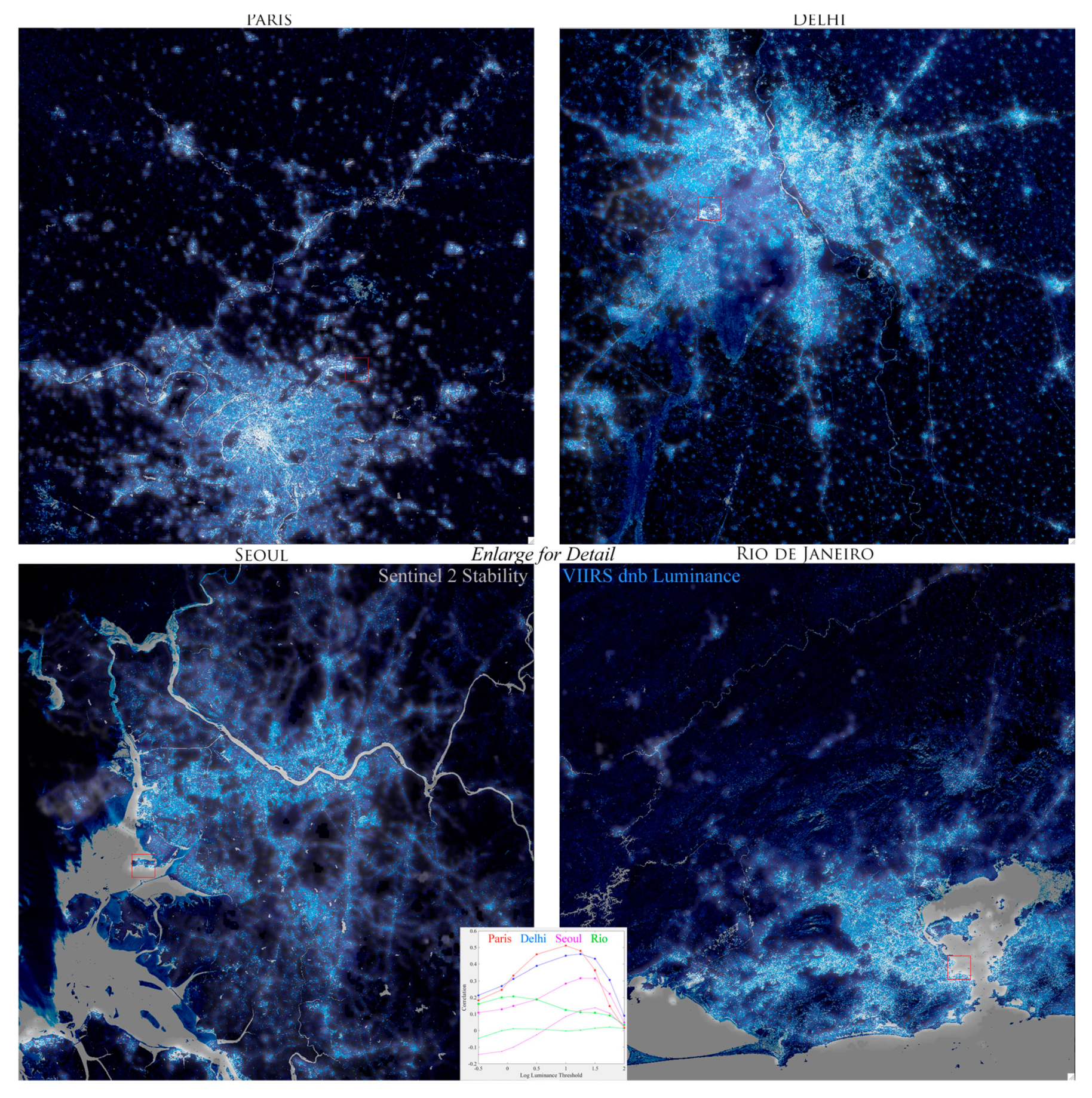
Comparison of VIIRS night light with Sentinel 2 Homogeneity and Variability metrics suggests that the spectral Stability metric may be used to identify an optimal low luminance threshold for which the spatial extent of higher stability areas corresponds to the spatial extent of the higher luminance areas. The spectral stability provides a single proxy for both homogeneity of impervious surface and persistence of building shadow. When compared to full range VIIRS luminance, some overglow is apparent extending beyond the most densely built areas with high spectral stability values. Progressively increasing the low luminance threshold attenuates the overglow and causes the more brightly lighted extents to shrink, more closely approximating the spatial extent of the higher stability values. This changing correspondence can be quantified by computing the spatial correlation between VIIRS luminance pixels above each threshold with Sentinel stability values. This is illustrated in Figure 7. As overglow is reduced, spatial correlation increases, until the more brightly lighted area becomes smaller than the more densely built up area and the correlation decreases. However, a common complication is illustrated in Figure 7 as each luminance threshold produces varying spatial agreement with different peripheral morphologies in different locations. The spatial correlation metric therefore represents an average of the overall spatial agreement of the luminance and built density. The generally low correlation values are partially a result of the spatial disparity between the 500 m VIIRS GIFOV and the 10 m Sentinel GIFOV and the greater spectral diversity within the VIIRS pixel in less densely built peripheral areas. It is also a result of the presence of water bodies which have very high spectral stability but are not lighted, thereby reducing the overall correlation. This is especially apparent in the cases of Seoul and Rio de Janeiro. The thin curves in Figure 7 show the full tile correlations for these two cities—including large areas of unlighted, but spectrally stable water. Using spatial subsets of each with large water areas excluded increases the overall correlation (thick curves) but does not change the peak correlation threshold. It is also noteworthy that each of the 4 examples shows peak correlation at a somewhat different low luminance threshold. This is consistent with the findings of [19] that no single threshold produces consistent agreement between DMSP-OLS lighted extent and Landsat-derived built area estimates.
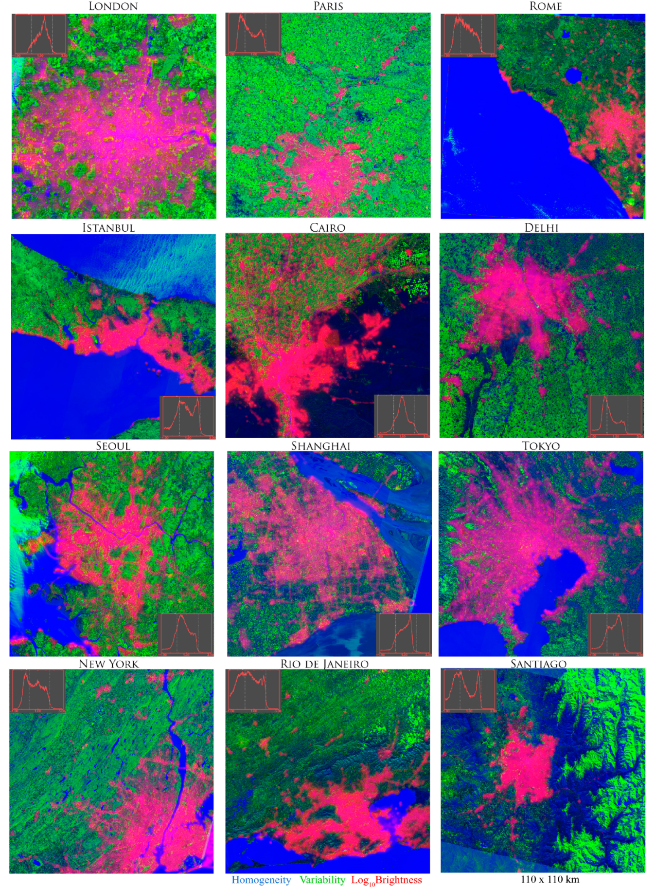
A key result of this analysis is the conflation of overglow and small dim light sources made clear by the Sentinel—VIIRS comparisons. In the RGB composites in Figure 6 the lower luminance levels (red) coincide with the higher spectral variability (green) and lower homogeneity (low blue) to show yellow peripheries surrounding the brighter, more homogeneous core areas in magenta (red + blue). As the density of spectrally stable impervious surface diminishes and the density of spectrally variable vegetation and soil increases toward the peripheries the luminance level decreases accordingly. However, the presence of overglow is clearly evident over water bodies in all the intercomparison sites. This ambiguity inherent in lower luminance levels is a serious limitation for DMSP [19], but must also be considered for VIIRS.
Compared to the full range of VIIRS dnb Log10 luminance values shown in Figure 4, the lower luminance pixels have clearly been attenuated in Figure 6 and Figure 7. As a result, the overglow is greatly reduced. However, what is less obvious is the complete attenuation of a great many smaller, dimmer light sources in areas that appear dark in the stretched composite. Figure 6 shows spectral luminance composites combining Log10 VIIRS dnb luminance (R) with multi-season spectral variability (G) and homogeneity (B). The correspondence of increasing luminance with decreasing temporal variability can be seen in both the spectral-temporal feature space, and on the composite images. The persistent magenta hue of the urban cores indicates that they are relatively homogenous (blue) and luminant (red), with consistently low temporal variability. In a couple of examples (e.g., Rome, Shanghai), a more yellow cast indicates greater seasonal variability presumably related to more finely dispersed vegetation and bare soil. However, in the suburbs west of NYC, the density and seasonal variability of the suburban forest is enough to suppress the low background luminance, suggesting that accurate depiction of forested suburban development may be a weakness of this approach.
The dual consequence of the low luminance ambiguity is that the thresholding process attenuates both overglow and small, low luminance light sources simultaneously. The relative amount, and effect, of each type of attenuation depends on the distribution and spatial configuration of bright and dim sources. The net effect of increasing the low luminance threshold is to reduce overglow around larger brighter sources, thereby representing their spatial extent more accurately, while simultaneously attenuating increasing numbers of smaller, dimmer sources, thereby underrepresenting them. The implication is that any analysis using VIIRS dnb to represent urban extent must take into account the effect of the low luminance threshold on the derived quantities. In this analysis, multiple thresholds are used, and results compared in the context of threshold sensitivity.
3.3. Progressive Evolution of Morphology and Spatial Network Structure
Spatial networks are generated using Log10 low luminance thresholds of −1.0, 0, 1.0, and 1.5 for each regional night light image. Areas and perimeters are computed for each spatially contiguous node (lighted settlement) on each network. Color-coded maps of network component size (km2) are shown in Figure 8 for the most extensive network corresponding to the lowest (least conservative) low luminance threshold (−1.0) in each case. Superimposed on these larger area extents are the corresponding smaller extents produced by a higher threshold of 1.0. These composite maps show both the bright urban cores and the dimmer network extents—but in terms of spatially contiguous area rather than brightness. This emphasizes the spatial contiguity of the networks that is difficult to see in traditional brightness maps. Based on comparison to the Sentinel 2 Stability maps, the −1 threshold can be seen to overestimate the spatial extent of urban land cover, while still eliminating large areas of low luminance overglow (e.g., over water). Conversely, the 1 threshold was found to underestimate built area in some, but not all, cases. The 1.5 threshold either bisects or completely attenuates the primary mode of most of the 12 distributions, thereby eliminating large lighted areas and leaving only the brightest urban cores. This suggests that a rigorous application of the progressive segmentation approach would use a set of at least 3 thresholds between the intermediate 0 and 1 thresholds (e.g., −0.25, 0.0, 0.25) and quantify the sensitivity of the segmentation maps and size distributions to the threshold chosen [10] and [11].
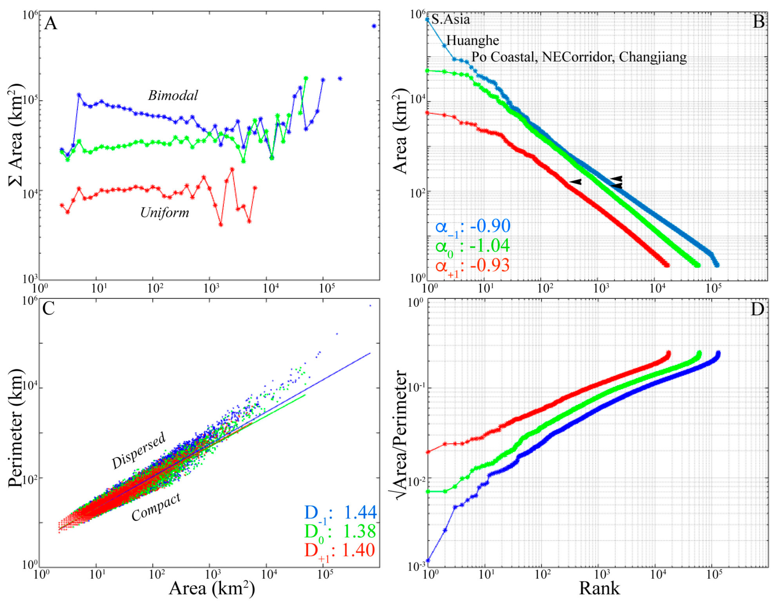
Distributions of segment areas and perimeters show a progressive evolution with decreasing low luminance threshold. Distributions calculated from each of the six regional VIIRS composites using four low luminance thresholds are shown inset on each of the network maps in Figure 8. The individual distributions are combined in Figure 9. The rank-size distributions (Figure 9B) are all linear spanning 4 to 5 orders of magnitude with slopes near unity (−0.9 to −1.04). This linearity with near unity slope implies equal areas across spatial scale of segment size. This is verified in the logarithmically binned ΣArea histograms in Figure 9A. The concavity of the rank-size distribution with the lower Log10 luminance threshold (−1) produces the bimodal distribution in the corresponding histogram indicating greater areas in the upper and lower tails than in the center of the distribution. The implications of this are discussed in detail below.
Area-perimeter distributions quantify the morphology of the segments resulting from different low luminance thresholds. The area-perimeter plot (Figure 9C) shows quasi-linear scaling over 3 to 5 orders of magnitude in both dimensions. However, the linearity and dispersion of the area–perimeter distributions change with luminance threshold. The lowest luminance threshold (−1) distribution shows some upward curvature, indicating that the morphology of the larger segments becomes increasingly complex as the luminance threshold approaches the lower end of the luminance distribution. Fractal dimension estimates, derived from the area-perimeter regression range from 1.38 to 1.44—consistent with the range of values obtained for the finer scale observations of Batty and Longley [2]. However, the distributions in Figure 9C represents much larger numbers of components and areas, including not only individual isolated settlements but also larger interconnected systems of settlements. For all three low luminance thresholds, some dispersion about the trend is apparent. The effect of the dispersion in the area-perimeter distribution can also be seen in the rank-shape plot (Figure 9D) derived from the sorted √Area/Perimeter distribution of all segments. This plot complements the rank-size plot in that it shows the progression from the simplest, near-circular segments (√A/P = 0.28) to more complex, crenulated segments with √A/P more than two orders of magnitude lower. While the highest luminance threshold shows a linear scaling of dimension over 3–4 orders of magnitude, the lowest threshold shows a clear downward curvature with multiple discontinuities approaching the highest fractal dimensions.
The effects of the progressive segmentation are apparent in comparison of the resulting rank-size distributions. As expected, in every case the lower tail (high rank, small size) shows the attenuation by reduced numbers and size of the smallest components in the distribution. However, increasing the low luminance threshold has varying effects on the larger components in the distribution. This can be seen by comparing the green and blue distributions in each case. In some cases, (e.g., China) the attenuation affects primarily the lower tail, while in others (e.g., Middle East, S. Asia) the reduction from the higher threshold propagates well into the middle of the distribution, or even into the upper tail (e.g., US Northeast Corridor). In contrast, the change from the intermediate (0) to higher (1) luminance threshold is more consistent across the regions; reducing both size and number of components by near equal amounts to produce a parallel shift from the second (green) to third (red) distribution. The effect of increasing the low luminance threshold on the lower and middle parts of the distribution results in attenuation and shrinkage (respectively) of the components of the network above threshold. The effect of increasing the threshold on the upper tail is fragmentation. This is seen in the profound changes in size of the largest components, particular in the case of South Asia where the giant component encompassing much of the subcontinent is fragmented into several smaller components.
The effects of the progressive segmentation on the slope estimates of the resulting rank-size distributions are largely as expected based on previous studies using DMSP. In cases where the effect is seen on components of all sizes, the entire distribution shifts in parallel. In the cases mentioned above, the effect may be primarily in the lower tail. Because the exponent fitting procedure works progressively from the upper tail down into the lower tail, the slope estimates apply only to the distribution above the cutoff (arrows on Figure 8), below which the misfit increases, and the plausibility of the power law characterization diminishes. This focus on the upper tail of the distribution is appropriate because the low luminance noise effectively imposes a detection limit, which makes the smaller, dimmer components of the network less reliable than the larger, brighter ones. In the case of South Asia, increasing the threshold fragments the giant component thereby producing a large number of smaller components and significantly increasing the slope from −0.8 to −1.0.
4. Discussion
Recent increases in both spatial and temporal resolution offered by Sentinel 2 and VIIRS fundamentally change our ability to characterize urban morphology and network structure relative to what was possible using Landsat and DMSP-OLS. Sentinel 2 can resolve individual buildings and roads that are manifest as mixed pixels in Landsat imagery. Relative to DMSP-OLS, VIIRS’ increased dynamic range and higher spatial resolution reduce overglow extent and resolve smaller, dimmer light sources.
4.1. Characterizing Urban Morphology and Network Structure
Combined use of rank-size (Area) and rank-shape (√Area/Perimeter) distributions provides a common basis for simultaneous characterization of urban morphology and spatial network structure. Whereas the area-perimeter distribution has been used extensively to quantify scaling properties and fractal dimensions of urban land cover at meter to hectometer scales (e.g., [2]), and rank-size distributions of urban populations have been used to quantify urban hierarchy (e.g., [27,28]) at national scales, the two concepts can be combined to characterize the full range of built environments in the context of evolving spatial networks of land use. By using contiguous area rather than administratively bounded population, administrative fragmentation is avoided and both size and shape of network components are referenced to common dimensions of length and area. The rank-size distribution quantifies the scaling properties of the network components with respect to area while the rank-shape distribution quantifies the scaling properties with respect to length and complexity of boundary.
The dispersion of the area-perimeter distribution reveals a size dependence in the scaling of shape and area of settlements. For all three thresholds shown in Figure 9C, the dispersion about the linear trend shows a significant range of perimeters for each segment area, indicating variation in shape. However, the dispersion increases with area for segments smaller than ~500 km2 then progressively diminishes for larger segments, which diverge upward from the regression line. The coalescence of large network components into larger more interconnected components reduces the variability of shape while simultaneously increasing the morphologic complexity (fractal dimension) of the largest network components. The implication is that the largest network components are more complex, with somewhat higher fractal dimension, than would be predicted by a single scaling law. Nonetheless, the quasi-linear nature of the area-perimeter plot over 5+ orders of magnitude suggests that the fractal nature of urban morphology extends from the scale of individual cities to include vastly larger spatial networks of interconnected settlements.
Distributions of network component size and shape together provide a basis for understanding the dynamic evolution of spatial networks through the combined processes of nucleation, growth and interconnection. In the lowermost tail of the rank-size distribution, new components come into existence through the process of nucleation. Components progress upward through the distribution toward the upper tail by a process of growth (e.g., radial, ballistic) at their peripheries. In the upper tail, the finite spatial domain leads to increasing dominance of interconnection as large components merge to form larger components. The scaling of the component shape, as given by the area–perimeter relations, is critical because components’ shapes determine the length of their periphery and therefore their potential for 2D growth by peripheral expansion or infill.
The slope and linearity of the rank-size distribution provides constraints on relative rates of nucleation, growth and interconnection. Distributions with slopes > −1 imply dominance by large numbers of small components in the lower tail. Distributions with slopes < −1 imply dominance by small numbers of large components in the upper tail. Slopes near −1 imply uniform area distribution across scales (e.g., Figure 9A). In a similar way, slope and linearity of rank-shape distributions provide independent constraints on the spatial form of growth. A more linear rank-shape distribution implies stricter scaling of fractal dimension, while greater downward curvature implies a progressive increase in complexity of shape—possibly suggesting a multifractal process. The slope and linearity of the rank-size distribution have clear implications for the process of urban growth because the persistence of a linear distribution with unity slope implies a balance between nucleation, growth and interconnection [11].
Combining rank-size and rank-shape distributions with progressive thresholding of continuous fields provides a partial solution to the problem of definition (discussed in the Introduction) by allowing comparison of scaling properties across multiple realizations of a single process. Consistency of distribution across thresholds suggests a scale-free process. Progressive change with threshold may suggest multiple processes. The latter may be relevant in the case of night light due to the similarity of luminance levels from diffuse sources and from overglow of bright sources.
Comparing the progression of rank-size and rank-shape distributions for the different regions shown in Figure 8 highlights differences in their network structures. The rank-size distributions for the Southeast Corridor of Brazil maintain linearity and near-unity slope over all but the lowest threshold, where the lower tail falls off at a greater slope. In the rank-shape distribution, the lowest threshold distribution shows a conspicuous drop in √Area/Perimeter for the largest 15 components reflecting the transition from smaller components with lower fractal dimension to larger, more dendritic components. In comparison, the US Northeast Corridor example shows the emergence of the giant component in both of the lower threshold distributions contrasting starkly with the dominance of the 7 largest cities in the most restrictive threshold distribution. The Western Europe and Middle East regions both show a strong disparity between the two lower threshold and two upper threshold distributions. This is manifest both by jumps in the size of component (over the full distribution) and jumps in the scaling of the largest few components in both regions. Both South Asia and China examples show the simultaneous emergence of giant components and the progressive expansion of the lower tail with the lowest threshold.
The abrupt transitions occurring at the lowest threshold for the South Asia and China networks raise an interesting question about the information content of the VIIRS night light. We know from spatiotemporal analysis of DMSP that night lights tend to get brighter as they grow larger in area [11,29]. If the presence of dim light is a predictor of future presence of brighter light as development intensifies, then the spatial networks corresponding to the lowest thresholds may suggest the spatial form and extent of future network development. If so, the implications could be particularly interesting in the case of interconnection of large components to form giant components in the future. The proximity of the Huanghe and Changjiang networks in China could suggest the emergence of a giant component interconnecting much of eastern China’s lighted development.
4.2. What VIIRS Reveals
The improved spatial resolution, geolocation, and dynamic range of the VIIRS dnb allows for mapping much smaller dimmer light sources than was possible with DMSP-OLS. Comparison of the VIIRS annual composite with astronaut photos from ISS confirms earlier local studies’ suggestions that the vast majority of light detected at hectometer scales originates from lighted road networks, suggesting that integrated brightness may serve as a proxy for road network density and the building density that generally accompanies it.
Different luminance thresholds reveal different manifestations of the built environment. The higher thresholds, admitting only the upper tail of the distribution, attenuate all but the brightest light, thereby showing the brightest, and generally most compact urban cores and infrastructure (e.g., airports, seaports, industrial complexes). Lower thresholds, admitting the upper mode of the distribution, increase the areal extent considerably by extending from the brightest cores to the large areas surrounding them. Still lower thresholds, admitting the lower mode of the distribution, increase the areal extent further by including larger numbers of smaller dimmer sources, as well as longer, more isolated high traffic road networks with sufficient traffic to be detected against a darker background. The multi-threshold maps in Figure 8 clearly show the disproportionate effect that the lowest threshold has on the connectivity of the spatial networks. This increase in connectivity is manifest as both the downward curvature and discontinuities in the rank-shape distributions and the emergence of giant components (e.g., S. Asia and NECorridor) of interconnected settlements spanning a wide range of sizes. The emergence of the largest, most complex network components at the lowest threshold illustrates the central role of transportation networks—both to the morphology of settlement networks and to material and human flows throughout the network.
4.3. The Nature of Light Sources
The fine detail seen in the astronaut photos in Figure 4 and other decameter-scale night light imagery (e.g., [30,31,32]) illustrate a challenge in interpretation of hectometer-scale night light imagery. In contrast to daytime measurements of reflected sunlight by most optical sensors, the aggregate radiance of night light measured for a single pixel is much less representative of the luminance of the full area of the IFOV. Even at a resolution of 1 m, most of the IFOV is generally dark so the sensor response is a result of a small number of very bright point sources—or perhaps just one. This is similar to the case of a single specular reflector dominating the reflectance of the IFOV in daytime optical imagery. In the case of hectometer-resolution sensors like VIIRS, the pixel response may be even more dominated by a few point sources and even less influenced by light scattered from ground surfaces. The implications of this bias are important for studies that infer causality from statistical analyses of hectometer to kilometer resolution night lights with other aggregate measures of potential correlates (e.g., land cover, GDP, population density).
The comparisons between VIIRS and the astronaut photos in Figure 6 confirm the importance of lighted streets and roads to the night light signal. Sub-meter night light imagery from Berlin Germany [30], Birmingham England [31], and Brisbane Australia [32] all clearly show lighted streets and roads as the principal source of the nocturnal radiance field. Lighted commercial, industrial, and residential spaces also contribute, but the astronaut photos in Figure 4 show that their spatial extent is significantly less than that of streets and roads. In all of these studies, the brightness distributions are dominated by small numbers of very bright point sources superimposed on a background of effectively dark pixels. The implication is that night light in built environments comes almost entirely from outdoor lighting rather than from light transmitted from within buildings, and that most of this light comes from streets and roads.
Unlike the DMSP-OLS night light composites, which show little more than monotonic luminance gradients and distributions, the greater dynamic range of the VIIRS composites reveals multiple distinct modes of the brightness distribution, corresponding to orders of magnitude differences in luminance of sources. This provides considerable additional information on intra-urban structure like transportation network density. The tails of the distributions also distinguish both the brightest sources and the decaying overglow at urban peripheries. While overglow gradients are modulated by source brightness, and there does not seem to be a single threshold that matches source boundaries in all of the 12 intercomparison sites, the range of brightnesses of the lower tail falloffs generally lie within the Log10 luminance range of −0.5 to 0.5, thereby providing far more spatial detail of network structure than the DMSP-OLS products. In addition, the lack of saturation of the brightest sources reveals far more internal structure of urban cores. However, spatial aliasing of this decameter scale internal structure by VIIRS’ hectometer resolution IFOV produces some incoherent variations in brightness that introduce spurious fractal structure to continuously developed areas that might be more accurately considered spatially contiguous. The result is an underestimation of total area for the lowest thresholds. This underestimation is generally reduced as thresholds increase and the structure of the most brightly lit infrastructure emerges from the background luminance. The fractal structure is therefore only partially a result of the underlying fractal land cover. It is also a result of the aliasing described above.
4.4. Contrasting Forms of Urban Morphology and Network Structure
Depiction of urban morphology by progressive segmentation of night light luminance provides two complementary perspectives on urban dynamics. Increasing the low luminance threshold reduces the full extent of the network to progressively reveal the structure connecting cores of greater luminance. As such, it provides an independent criterion to describe internal structure of continuously developed areas that may not be apparent from optical imagery—even with the resolution of Sentinel 2. For example, it can provide partial proxies for road density, public infrastructure investment or energy consumption. In a complementary sense, decreasing the low luminance threshold progressively reveals the evolving structure of the network, and potentially future growth patterns—if present day luminance is a predictor of more intensive future development. Spatiotemporal analyses of DMSP-OLS data suggest that this has often been the case in the past decades [29].
5. Conclusions
Multi-season spectral characteristics of built environments associated with urban development provide an independent complement to the night light brightness that is increasingly being used for spatial analysis of urban systems. The benefit of spectral properties derived from Sentinel 2 imagery is primarily related to its 10 m resolution and frequent revisit—making it possible to use seasonal variation in reflectance characteristics as proxies for physical properties associated with the diversity of built environments worldwide. Specifically, high fractions of spectrally stable impervious surface combined with persistent deep shadow between buildings. Direct comparisons of multi-season spectral stability from Sentinel with night light brightness from VIIRS show better spatial agreement and more detailed representation of a wide range of built environments than was possible using Landsat and DMSP-OLS. However, these comparisons also show location-specificity in the spectral homogeneity and variability of different intercomparison sites. As with DMSP and Landsat, the cross-sensor comparisons suggest that no single low luminance threshold for VIIRS provides optimal spatial correspondence to built extent derived from Sentinel in different urban systems. This, combined with the continuous and fractal scaling nature of urban land cover suggests that the most informative way to use these data sources together may be through progressive segmentation of both to characterize the evolving spatial networks of the properties associated with each. A simple 4 threshold comparison of 6 regional night light networks shows consistent scaling behavior spanning 3 to 5 orders of magnitude in size and number with rank-size slopes consistently near −1—suggesting a dynamic balance among the processes of nucleation, growth and interconnection [11]. The same thresholds yield rank-shape distributions that reveal progressive non-linear decreases in √Area/Perimeter with increasing size, transitioning abruptly to larger, higher dimensional networks for the lowest thresholds. In part, this may be due to a dual origin for low luminance from both diffuse sources and overglow from bright sources. However, the changes in the slopes with decreasing low luminance threshold also reveal systematic differences among these systems that may inform our understanding of the spatiotemporal evolution of urban development going forward.
Funding
This research was funded by the NASA Multisensor Land Imaging Program (grant NNX15AT65G).
Acknowledgments
The author is grateful to D. Sousa, C. Elvidge, C. Milesi, X. Li, Q. Zhang, B. Yu, D. Balk, M. Montgomery, G. Henebry, M. Friedl and D. Roy for thought-provoking discussions on some the topics discussed here. Thanks to A. Clauset and colleagues for developing the power law estimation methodology and sharing the software.
Conflicts of Interest
The author declares no conflict of interest.
References
- Mesev, V.; Longley, P.; Batty, M.; Xie, Y. Morphology from imagery: Detecting and measuring the density of urban land use. Environ. Plan. A 1995, 27, 759–780. [Google Scholar] [CrossRef]
- Batty, M.; Longley, P. Fractal Cities; Academic Press: London, UK; San Diego, CA, USA, 1996; p. 394. [Google Scholar]
- Mesev, V. Remotely Sensed Cities—An Introduction; CRC Press: London UK, 2003; p. 433. [Google Scholar]
- Deuskar, C. What does urban mean? In Sustainable Cities; World Bank: Washington, DC, USA, 2015. [Google Scholar]
- Forster, B.C. An examination of some problems and solutions in monitoring urban areas from satellite platforms. Int. J. Remote Sens. 1985, 6, 139–151. [Google Scholar] [CrossRef]
- Small, C. The Color of Cities: An Overview of Urban Spectral Diversity. In Global Mapping of Human Settlements; Herold, M., Gamba, P., Eds.; Taylor and Francis: Didecott, UK, 2009; pp. 59–106. [Google Scholar]
- Du, P.; Liu, P.; Xia, J.; Feng, L.; Liu, S.; Tan, K.; Cheng, L. Remote Sensing Image Interpretation for Urban Environment Analysis: Methods, System and Examples. Remote Sens. 2014, 6, 9458–9474. [Google Scholar] [CrossRef] [Green Version]
- Auerbach, F. Das Gesetz der Bevolkerungskonzentration. Petermanns Geogr. Mitt. 1913, 59, 74–76. [Google Scholar]
- Soo, K.T. Zipf’s Law for cities: A cross-country investigation. Reg. Sci. Urban Econ. 2005, 35, 239–263. [Google Scholar] [CrossRef]
- Small, C.; Elvidge, C.D.; Balk, D.; Montgomery, M. Spatial Scaling of Stable Night Lights. Remote Sens. Environ. 2011, 115, 269–280. [Google Scholar] [CrossRef]
- Small, C.; Sousa, D. Spatial Scaling of Land Cover Networks. arXiv 2015, arXiv:1512.01517. [Google Scholar]
- Elvidge, C.D.; Baugh, K.; Zhizhin, M.; Hus, F.C.; Ghosh, T. VIIRS night-time lights. Int. J. Remote Sens. 2017, 38, 5860–5879. [Google Scholar] [CrossRef]
- Elvidge, C.D.; Baugh, K.E.; Zhizhin, M.; Hsu, F.C. Why VIIRS data are superior to DMSP for mapping nighttime lights. In Proceedings of the Asia-Pacific Advanced Network, Honolulu, HI, USA, 13–16 January 2013; Volume 35, pp. 62–69. [Google Scholar]
- Small, C. Multisource Imaging of Urban Growth and Infrastructure Using Landsat, Sentinel and SRTM. In Proceedings of the NASA Landsat-Sentinel Science Team Meeting, Rockville, MD, USA, 3–5 April 2018. [Google Scholar]
- Small, C.; Nghiem, S.V. A continuous infrastructure index for mapping human settlements. In Proceedings of the NASA Multi-source Land Imaging Landsat-Sentinel Science Team Meeting, Bethesda, MD, USA, 20–21 April 2016. [Google Scholar]
- Small, C.; Machado, R.P.P.; Barrozo, L.V.; Luchiari, A. Mapping decades of urban growth and development with multi-temporal spectral mixture models. In Proceedings of the XVII SBSR—Simpósio Brasileiro de Sensoriamento Remoto, João Pessoa, Brazil, 25–29 April 2015. [Google Scholar]
- Small, C.; Milesi, C.; Elvidge, C.; Baugh, K.; Henebry, G.M.; Nghiem, S.V. The Land Cover Continuum; Multi-sensor Characterization of Human-Modified Landscapes. In Proceedings of the EARSeL/NASA Joint Workshop on Land Use and Land Cover Berlin, Berlin, Germany, 17–18 March 2014. [Google Scholar]
- Small, C.; Okujeni, A.; Van der Linden, S.; Waske, B. Remote Sensing of Urban Environments. In Comprehensive Remote Sensing; Liang, S., Ed.; Elsevier: Oxford, UK, 2018; Volume 6, pp. 96–127. [Google Scholar]
- Small, C.; Pozzi, F.; Elvidge, C.D. Spatial analysis of global urban extent from DMSP-OLS night lights. Remote Sens. Environ. 2005, 96, 277–291. [Google Scholar] [CrossRef]
- Small, C.; Sousa, D. Humans on Earth: Global Extents of Anthropogenic Land Cover from Remote Sensing. Anthropocene 2016, 14, 1–33. [Google Scholar] [CrossRef]
- Clauset, A.; Shalizi, C.R.; Newman, M.E.J. Power-law distributions in empirical data. SIAM Rev. 2009, 51, 661–703. [Google Scholar] [CrossRef]
- Imhoff, M.L.; Lawrence, W.T.; Elvidge, C.D.; Paul, T.; Levine, E.; Privalsky, M.V. Using nighttime DMSP/OLS images of city lights to estimate the impact of urban land use on soil resources in the United States. Remote Sens. Environ. 1997, 59, 105–117. [Google Scholar] [CrossRef]
- Elvidge, C.D.; Baugh, K.E.; Kihn, E.A.; Kroehl, H.W.; Davis, E.R. Mapping city lights with nighttime data from the DMSP Operational Linescan System. Photogramm. Eng. Remote Sens. 1997, 63, 727–734. [Google Scholar]
- Levin, N.; Zhang, Q. A global analysis of factors controlling VIIRS nighttime light levels fromdensely populated areas. Remote Sens. Environ. 2017, 190, 366–382. [Google Scholar] [CrossRef]
- Small, C.; Elvidge, C.D.; Baugh, K. Mapping urban structure and spatial connectivity with VIIRS and OLS night light imagery. In Proceedings of the Joint Urban Remote Sensing Event, Sao Paulo, Brazil, 21–23 April 2013; pp. 230–233. [Google Scholar]
- Yu, B.; Tang, M.; Wu, Q.; Yang, C.; Deng, S.; Shi, K.; Peng, C.; Wu, J.; Chen, Z. Urban Built-Up Area Extraction From Log- Transformed NPP-VIIRS Nighttime Light Composite Data. IEEE Geosci. Remote Sens. Lett. 2018, 15, 1279–1283. [Google Scholar] [CrossRef]
- Batty, M. Hierarchy in Cities and City Systems. In Hierarchy in Natural and Social Sciences; Pumain, D., Ed.; Springer: Berlin/Heidelberg, Germany, 2006; Volume 3, pp. 143–168. [Google Scholar]
- Pumain, D. Alternative explanations of hierarchical differentiation in urban systems. In Hierarchy in Natural and Social Sciences; Pumain, D., Ed.; Springer: Berlin/Heidelberg, Germany, 2006; Volume 3, pp. 169–222. [Google Scholar]
- Small, C.; Elvidge, C.D. Night on Earth: Mapping decadal changes of anthropogenic night light in Asia. Int. J. Appl. Earth Obs. Geoinf. 2013, 22, 40–52. [Google Scholar] [CrossRef] [Green Version]
- Kuechly, H.U.; Kyba, C.C.M.; Ruhtz, T.; Lindemann, C.; Wolter, C.; Fischer, J.; Hölker, F. Aerial survey and spatial analysis of sources of light pollution in Berlin, Germany. Remote Sens. Environ. 2012, 126, 39–50. [Google Scholar] [CrossRef]
- Hale, J.D.; Davies, G.; Fairbrass, A.J.; Matthews, T.J.; Rogers, C.D.F.; Sadler, J.P. Mapping Lightscapes: Spatial Patterning of Artificial Lighting in an Urban Landscape. PLoS ONE 2013, 8, e61460. [Google Scholar] [CrossRef]
- Levin, N.; Johansen, K.; Hacker, J.M.; Phinn, S. A new source for high spatial resolution night time images—The EROS-B commercial satellite. Remote Sens. Environ. 2014, 149, 1–12. [Google Scholar] [CrossRef]
Figure 1.
Global networks of night light and land cover. VIIRS dnb brightness superimposed on MODIS false color composite shows the wide range of biomes hosting lighted development in 2019. The full extent of human habitation is considerably greater than suggested by anthropogenic night light. Boxes show approximate extents of regional analyses.

Figure 2.
Sentinel 2 VNIR composites of 12 urban systems and surrounding land cover networks. Inset boxes spanning urban cores give extents of full resolution subsets shown in Figure 3. Equivalent stretches highlight spectral diversity within and among urban cores. Low solar elevations emphasize shadow and topography.

Figure 3.
Sentinel 2 VNIR composites of 12 urban cores shown in Figure 2 Equivalent stretches highlight spectral diversity within and among urban cores. Viewed at full 10 m resolution, individual buildings and streets are clearly distinguished in most, but not all, examples. Low solar elevations emphasize shadow and topography.

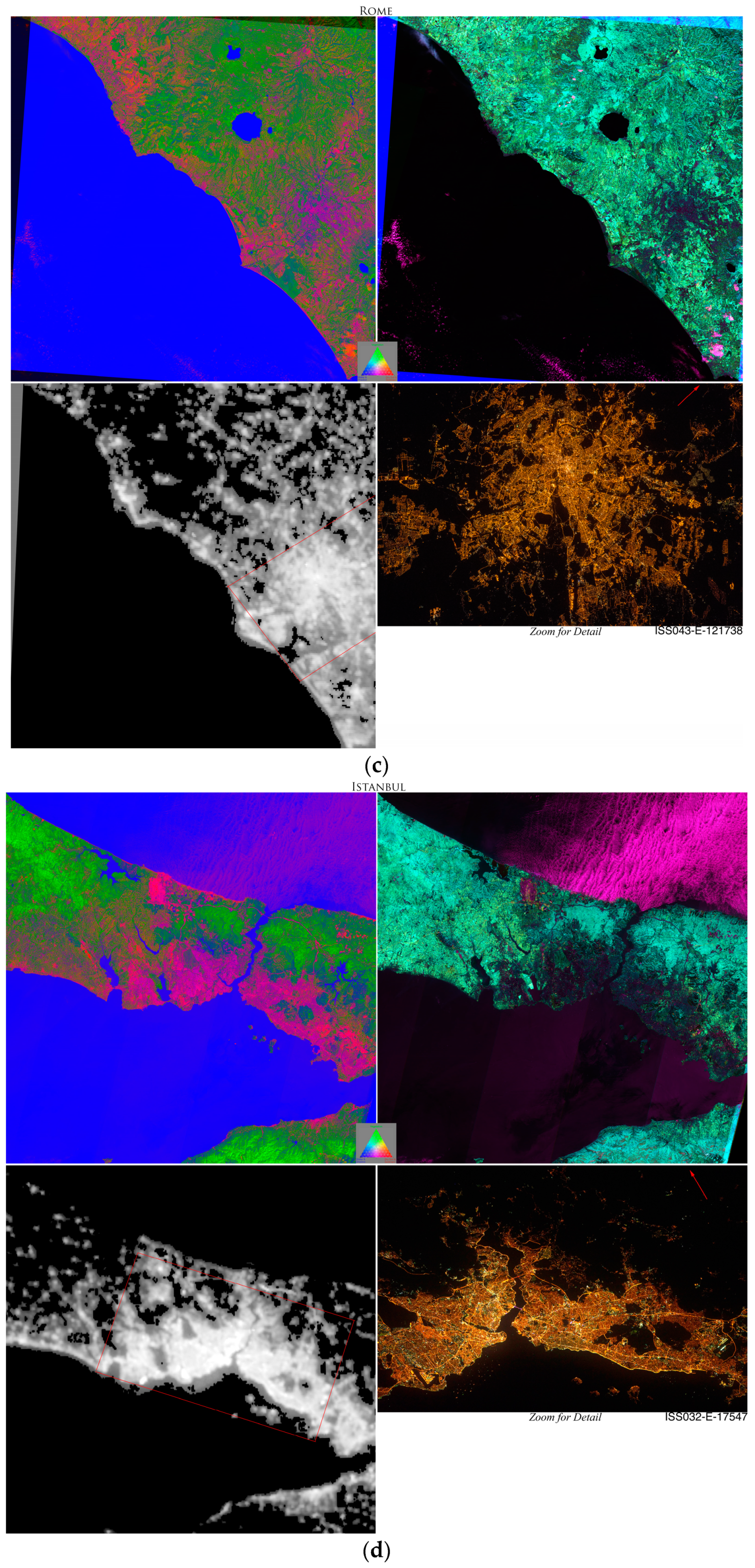
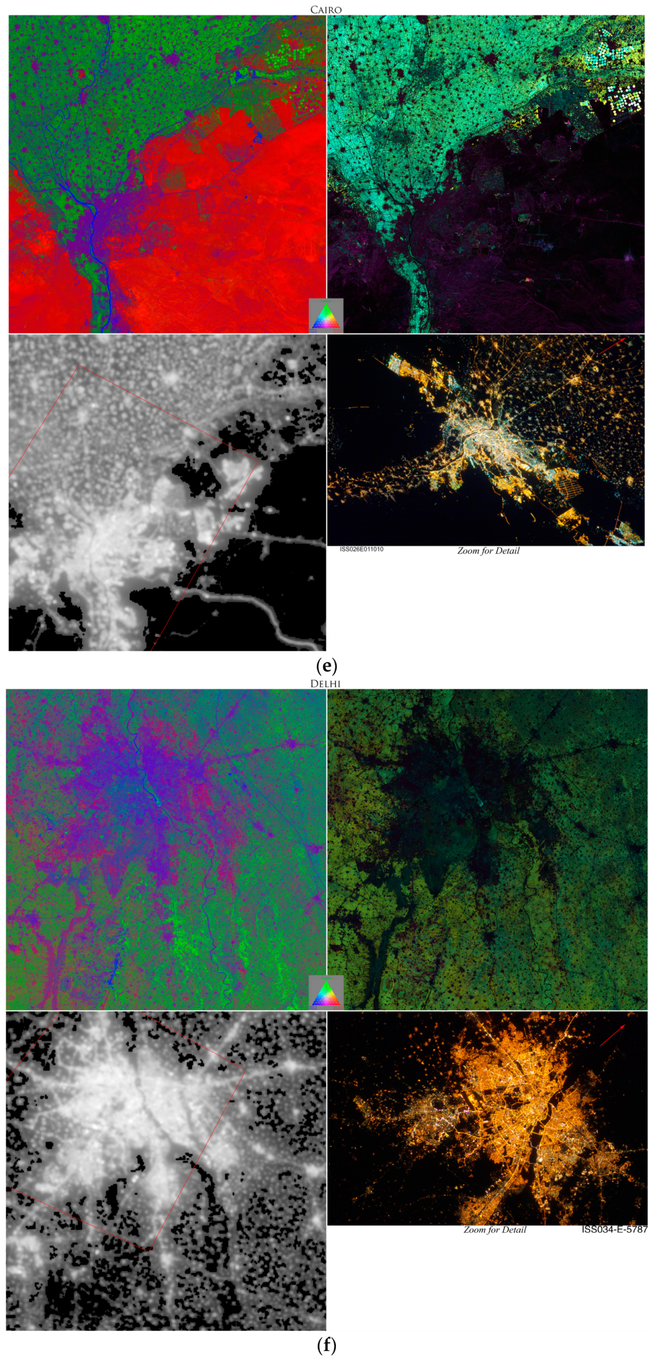
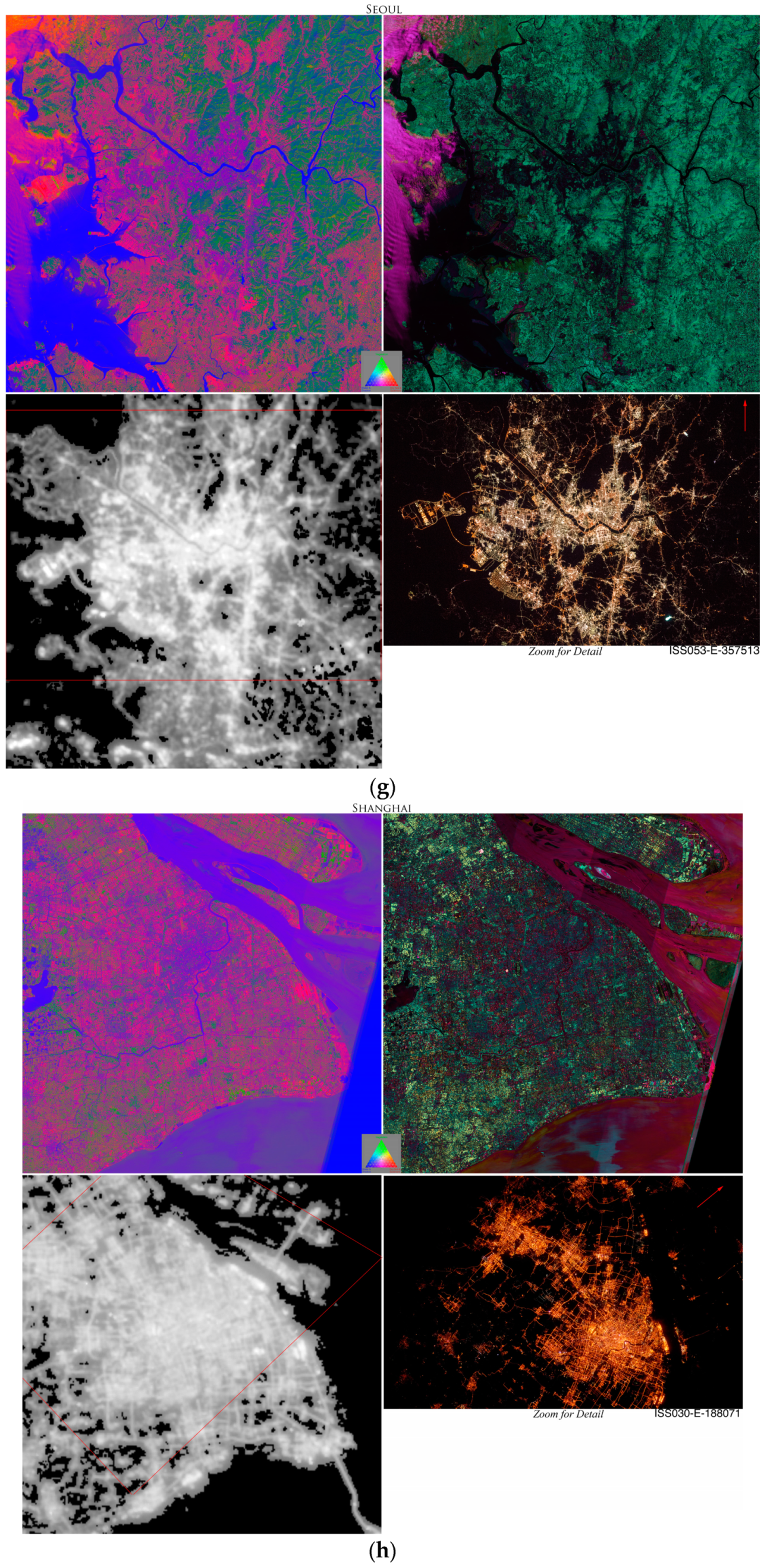
Figure 4.
Multi-season land cover composites and night light for 12 intercomparison sites. Seasonal mean (UL) and variability (UR) of Substrate, Vegetation and Dark fractions from Sentinel 2 clearly distinguish most densely built up areas as mixtures of shadow and impervious substrate. VIIRS dnb composite (LL) shows these areas are also brightly lighted. Astronaut photograph (LR) indicates that most bright light comes from road networks. Sites are: (a) London, (b) Paris, (c) Rome, (d) Istanbul, (e) Cairo, (f) Delhi, (g) Seoul, (h) Shanghai, (i) Tokyo, (j) New York, (k) Rio de Janeiro, (l) Santiago.


Figure 5.
Spectral stability spaces of 12 urban systems and surrounding land cover networks. In every example, maximum seasonal variability of reflectance decreases as spatial homogeneity of mixed pixels increases. The most stable (lower right apex) are water bodies, then urban cores with persistent deep shadow, while the most variable are mixtures of seasonal vegetation and soils of varying moisture contents. Aggregate land cover reflectance and illlumination vary continuously in space and time but seasonal variability always decreases with increasing building density.

Figure 6.
Spectral luminance composites of 12 urban systems and surrounding land cover networks. Inset histograms show clipping thresholds on Log10 luminance distributions of VIIRS dnb. A low luminance threshold of 0.25 generally attenuates overglow over water to match shorelines but diffusion of luminance on more crenulated boundaries (yellow) overestimates spatial extent of high homogeneity/low variability build up from Sentinel.

Figure 7.
Spectral stability and night light. Progressive increase of VIIRS dnb Log10 low luminance threshold attenuates dimmer light and reduces overglow. As overglow is reduced, spatial correlation with Sentinel spectral stability generally increases (inset) until lighted area becomes smaller than built area and correlation decreases. Note different optimal threshold for each location. A common threshold of 0 shows general agreement of cores with varying amount of overglow at coastlines.

Figure 8.
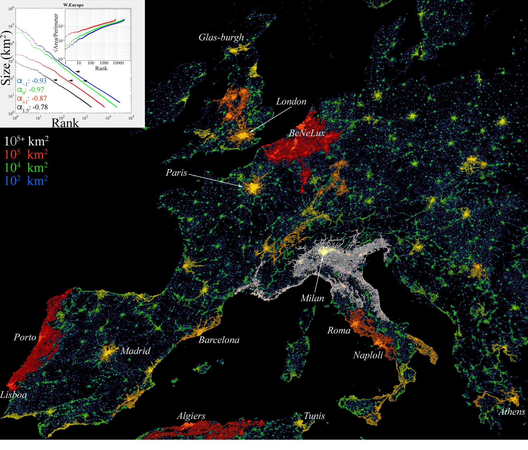
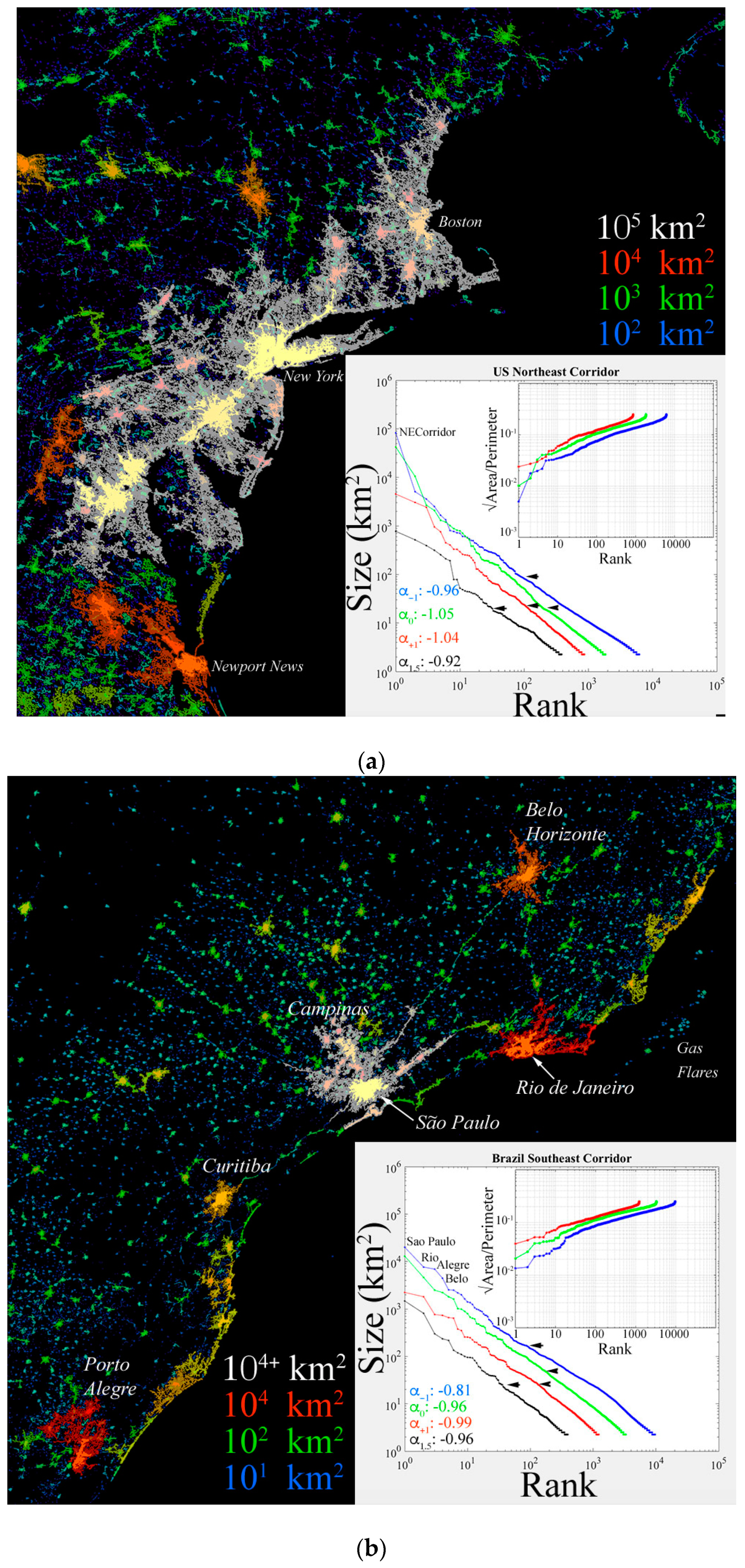
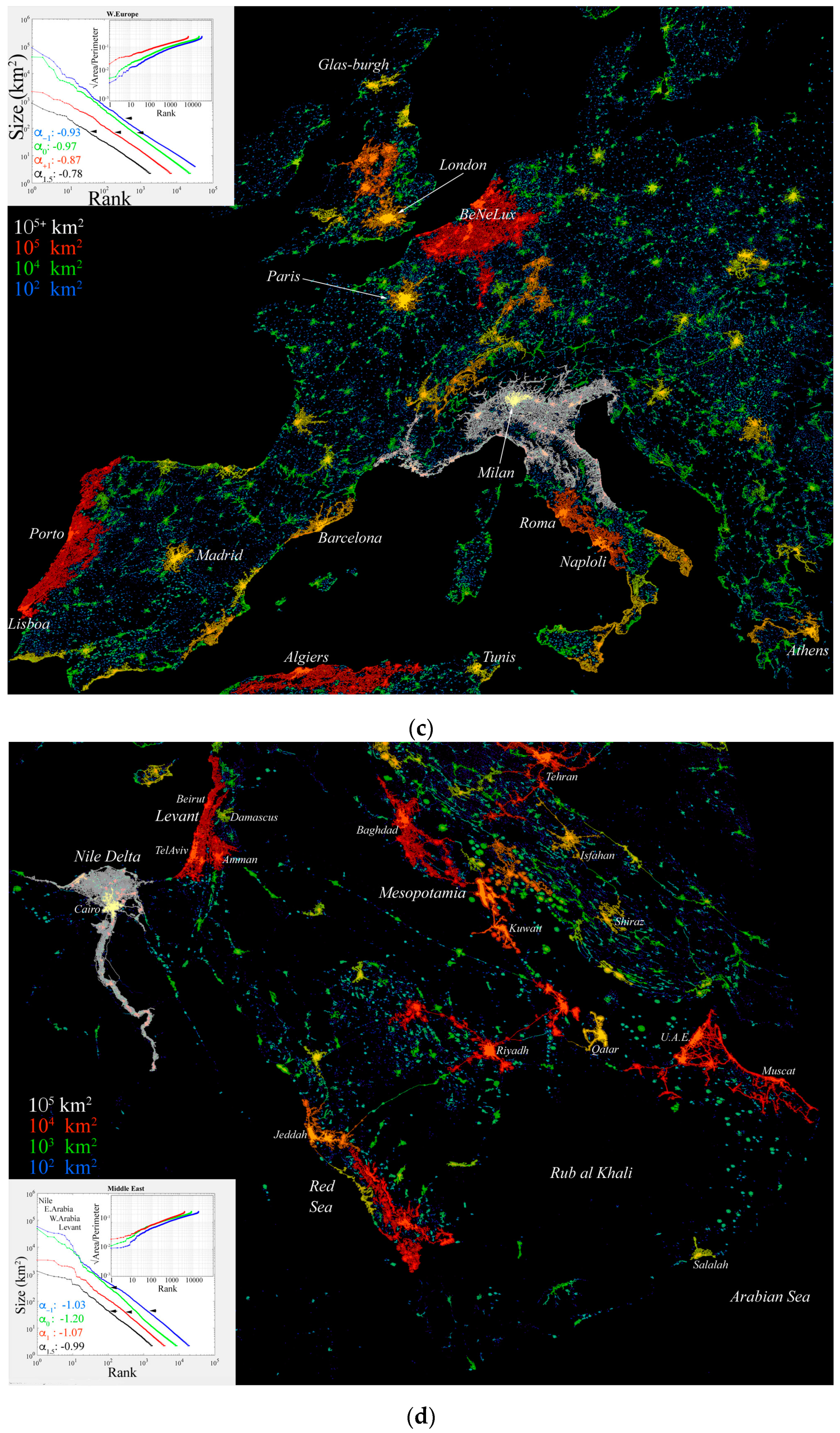
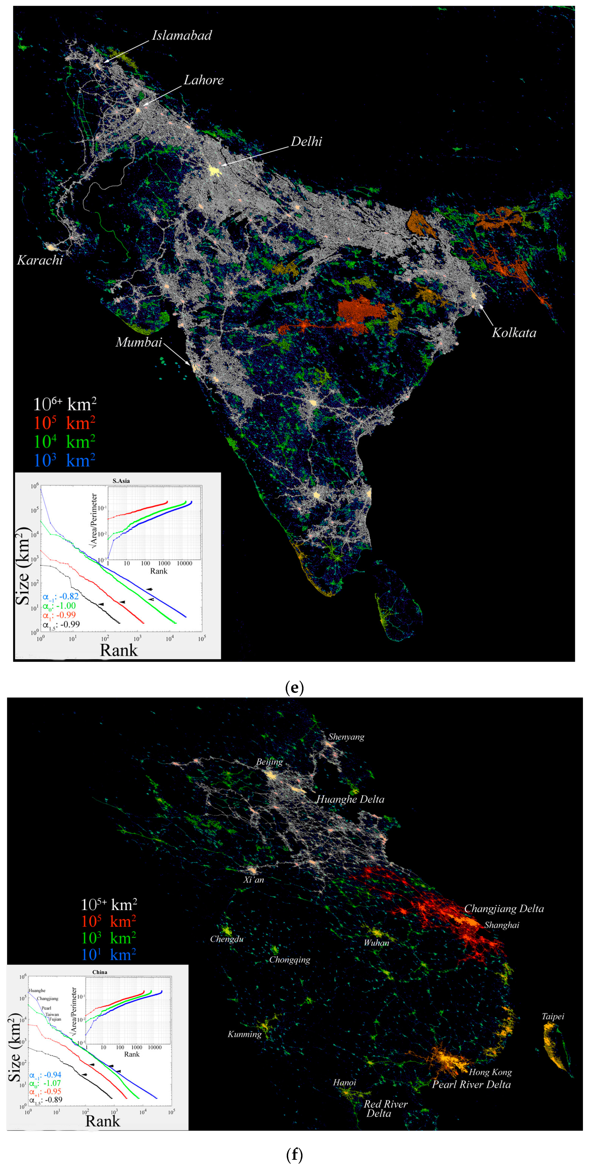
Network component maps and luminance threshold distributions for six regional examples. Background map shows bounding network component size for lower 10−1 brightness threshold. Foreground map shows smaller bounded component size for higher 10+1 threshold. Size color legend given for larger bounding components. Inset distributions and slope estimates show effect of progressive thresholding on size (area) and shape (√area/perimeter) of network components. Optimal lower tail cutoffs for slope estimates shown by arrows. Enlarge for additional detail. (a) Network component maps and luminance threshold distributions for the Northeast Corridor of the USA. Note the appearance of a single giant component (white) for the lowest threshold. (b) Network component maps and luminance threshold distributions for the Southeast Corridor of Brazil. The rank-size distribution for the lowest threshold (blue) shows the Rio de Janeiro and Porto Alegre components of similar size while the rank-shape distribution shows the Rio de Janeiro and São Paulo components of similar fractal dimension. (c) Network component maps and luminance threshold distributions for Western Europe. Note marked difference between distributions for Log10 luminance thresholds of 0 (green) and +1 (red). (d) Network component maps and luminance threshold distributions for the Middle East. Note the similarity of size and fractal dimension of the largest components in comparison to the clear hierarchy of the Western European components seen in (c). (e) Network component maps and luminance threshold distributions for South Asia. Note how the formation of a single giant component (white) for the lowest threshold affects the shape and slope of the corresponding rank-size distribution. (f) Network component maps and luminance threshold distributions for Eastern China and Northern Vietnam. Note the effect of the lowest threshold (blue) on the upper and lower tails of the rank-size distribution.
Figure 8.
Network component maps and luminance threshold distributions for six regional examples. Background map shows bounding network component size for lower 10−1 brightness threshold. Foreground map shows smaller bounded component size for higher 10+1 threshold. Size color legend given for larger bounding components. Inset distributions and slope estimates show effect of progressive thresholding on size (area) and shape (√area/perimeter) of network components. Optimal lower tail cutoffs for slope estimates shown by arrows. Enlarge for additional detail. (a) Network component maps and luminance threshold distributions for the Northeast Corridor of the USA. Note the appearance of a single giant component (white) for the lowest threshold. (b) Network component maps and luminance threshold distributions for the Southeast Corridor of Brazil. The rank-size distribution for the lowest threshold (blue) shows the Rio de Janeiro and Porto Alegre components of similar size while the rank-shape distribution shows the Rio de Janeiro and São Paulo components of similar fractal dimension. (c) Network component maps and luminance threshold distributions for Western Europe. Note marked difference between distributions for Log10 luminance thresholds of 0 (green) and +1 (red). (d) Network component maps and luminance threshold distributions for the Middle East. Note the similarity of size and fractal dimension of the largest components in comparison to the clear hierarchy of the Western European components seen in (c). (e) Network component maps and luminance threshold distributions for South Asia. Note how the formation of a single giant component (white) for the lowest threshold affects the shape and slope of the corresponding rank-size distribution. (f) Network component maps and luminance threshold distributions for Eastern China and Northern Vietnam. Note the effect of the lowest threshold (blue) on the upper and lower tails of the rank-size distribution.


Figure 9.
Aggregate urban morphology and network structure parameters of 6 geographic regions from VIIRS. Low luminance thresholds of −1, 0 and 1 (blue, green, red) yield consistent distributions. (A) Binned area histograms show near uniform Σ area distributions spanning 3 to 5 orders of magnitude in component size. (B) Rank-size distributions are linear, with slopes (α) near −1, but slightly concave for the lowest threshold. (C) Area-Perimeter plots scale over 3 to 5 orders of magnitude in component size with nearly identical slopes (fractal dimensions) but significant dispersions about trend line for smaller components, converging to higher dimension for the larger components. (D) Rank-shape distributions show increasing curvature with lower luminance threshold and considerably higher dimensionality for largest networks. Diversity of individual fractal dimensions in (C) and (D) exceed mean A/P estimates.


Table 1.
Sentinel 2 Tiles and Dates.
| City | Y | M | D | Tile | City | Y | M | D | Tile |
|---|---|---|---|---|---|---|---|---|---|
| London | 2016 | 06 | 06 | T30UXC-UYC | Delhi | 2016 | 06 | 04 | T43RFM-RGM |
| London | 2016 | 09 | 11 | T30UXC-UYC | Delhi | 2016 | 10 | 22 | T43RFM-RGM |
| London | 2017 | 01 | 02 | T30UXC-UYC | Delhi | 2016 | 12 | 21 | T43RFM-RGM |
| London | 2017 | 04 | 09 | T30UXC-UYC | Seoul | 2016 | 04 | 08 | T52SBG-SCG |
| Paris | 2016 | 12 | 27 | T31UDQ | Seoul | 2017 | 01 | 03 | T52SBG-SCG |
| Paris | 2017 | 01 | 26 | T31UDQ | Seoul | 2017 | 05 | 03 | T52SBG-SCG |
| Paris | 2017 | 05 | 26 | T31UDQ | Seoul | 2017 | 09 | 20 | T52SBG-SCG |
| Paris | 2017 | 11 | 22 | T31UDQ | Shanghai | 2017 | 02 | 28 | T51RUQ |
| Paris | 2018 | 02 | 25 | T31UDQ | Shanghai | 2017 | 04 | 29 | T51RUQ |
| Rome | 2015 | 08 | 30 | T32TQM | Shanghai | 2017 | 04 | 29 | T51RUQ |
| Rome | 2015 | 12 | 18 | T33TTG | Shanghai | 2017 | 12 | 20 | T51RUQ |
| Rome | 2016 | 08 | 04 | T323TQM | Tokyo | 2017 | 02 | 07 | T54SUE-SVE |
| Rome | 2017 | 01 | 01 | T33TTG | Tokyo | 2017 | 05 | 08 | T54SUE-SVE |
| Rome | 2017 | 04 | 02 | T33TTG | Tokyo | 2017 | 11 | 29 | T54SUE-SVE |
| Istanbul | 2016 | 02 | 08 | T35TPF | New York | 2015 | 09 | 24 | T18TWL |
| Istanbul | 2016 | 04 | 18 | T35TPF | New York | 2016 | 03 | 12 | T18TWL |
| Istanbul | 2017 | 05 | 03 | T35TPF | New York | 2016 | 10 | 18 | T18TWL |
| Istanbul | 2017 | 07 | 12 | T35TPF | Rio de Janeiro | 2017 | 03 | 10 | T23KPQ |
| Istanbul | 2017 | 09 | 10 | T35TPF | Rio de Janeiro | 2017 | 06 | 18 | T23KPQ |
| Cairo | 2015 | 09 | 02 | T36RUU | Rio de Janeiro | 2017 | 09 | 06 | T23KPQ |
| Cairo | 2016 | 03 | 10 | T36RUU | Santiago | 2016 | 03 | 05 | T19HCC-HCD |
| Cairo | 2016 | 04 | 19 | T36RUU | Santiago | 2016 | 08 | 02 | T19HCC-HCD |
| Delhi | 2016 | 02 | 05 | T43RFM-RGM | Santiago | 2016 | 12 | 20 | T19HCC-HCD |
© 2019 by the author. Licensee MDPI, Basel, Switzerland. This article is an open access article distributed under the terms and conditions of the Creative Commons Attribution (CC BY) license (http://creativecommons.org/licenses/by/4.0/).
Share and Cite
MDPI and ACS Style
Small, C. Multisensor Characterization of Urban Morphology and Network Structure. Remote Sens. 2019, 11, 2162. https://0-doi-org.brum.beds.ac.uk/10.3390/rs11182162
AMA Style
Small C. Multisensor Characterization of Urban Morphology and Network Structure. Remote Sensing. 2019; 11(18):2162. https://0-doi-org.brum.beds.ac.uk/10.3390/rs11182162
Chicago/Turabian StyleSmall, Christopher. 2019. "Multisensor Characterization of Urban Morphology and Network Structure" Remote Sensing 11, no. 18: 2162. https://0-doi-org.brum.beds.ac.uk/10.3390/rs11182162
Note that from the first issue of 2016, this journal uses article numbers instead of page numbers. See further details here.