Dip Filter and Random Noise Suppression for GPR B-Scan Data Based on a Hybrid Method in f - x Domain

Abstract

Ground-penetrating radar (GPR) is a close-range remote-sensing tool applied in a great many near-surface projects for engineering or environmental purposes. In GPR B-scans, there may exist a variety of reflections and diffractions that corresponds to different structures and targets in the subsurface media, and the noise is always embedded. To assist in the interpretation, GPR B-scans can be generally divided into two parts according to the dip attribute of the reflections, where the sub-horizontal layers and dipping structures are properly separated. In this work, we extend the f - x empirical mode decomposition (f - x EMD) to form a semi-adaptive dip filter for GPR data. In f - x domain, each frequency slice is decomposed by EMD and reconstructed to form a dipping profile and a horizontal profile respectively, where the reflections at different dips are separated adaptively. Then the noises mixed in the dipping profile are further separated by rank-deduction methods in f - x domain. The above two-step scheme constitutes the hybrid scheme, which can separate the dipping structures, sub-horizontal layers, and most of the random noise in GPR B-scans. We briefly review the basics of the f - x EMD, and then introduce the derived hybrid scheme in f - x domain. The proposed method is tested by the synthetic data, the forward simulation data, and the field data, respectively.

1. Introduction

Ground-penetrating radar (GPR) has been one of the most significant geophysical techniques and applied in a great many near-surface projects for engineering or environmental purposes. It features the non-invasive way of prospecting and the high resolution of the observed data [1,2]. As to most of practical GPR applications, processing and interpreting 2D GPR profiles (i.e., GPR B-scans) are one of the main tasks. In a GPR B-scan profile, there may be the reflections of the subsurface layers, the target objectives (e.g., rebars or metal pipelines), and various geological structures such as faults and fractures, etc. [3]. As to different prospecting purposes, all the above contents can be the targets of the survey, and the noise is inevitably mixed into the GPR data during acquisition due to the unstable equipment conditions. In some cases, these complex contents in the B-scans are not easy to identify, and the interpretation work may be time-consuming and relies on the skilled interpreters in their experience. So, if the reflections of the different structures and targets in the subsurface media, as well as the embedded noise can be separated according to the dip attributes or features, it is beneficial to the post-processing steps and the interpretation work.

There are several commonly accepted methods for separating the layers or events at different dips in GPR B-scan profiles. The simplest solution is to use the statistical properties, such as the “dip filter” modularized in some GPR software [4,5] based on the spatial mean filter within a sliding window [6]. It can simply highlight the sub-horizontal components in the B-scan, and the residual profile corresponds to the reflections that dip at high angles. The limit of this method is that the separation effect depends on the selection of the chosen window width, and the whole profile is processed by one standard once the parameter is decided. Moreover, when the GPR B-scans are transformed to the frequency-wavenumber (f - k) domain [7,8] or the linear Radon ($\tau$-p) domain [9], the components or events at different dips can be extracted or filtered by some designed filters. With the introduction of the directional wavelets, such as the curvelet transform [10,11] and the shearlet transform [12], some more substantial progress has been made. However, the methods in the transform or wavelets domain share a common problem that it is inconvenient and fallible to set the filter parameters, and the scheme thus appears to be not intuitive.

To avoid the process of adjusting filter parameters, Bekara et al. [13] applied the empirical mode decomposition (EMD) to replace the filters in the frequency-spatial domain, and referred to it as the frequency-spatial EMD or the f - x EMD. The classical EMD algorithm has played an important role in handling the non-stationarity of the signal since its introduction [14], and in the f - x EMD scheme, the frequency slice can be adaptively decomposed into a set of sub-components termed intrinsic mode functions (IMFs) by EMD. The f - x EMD was proposed for seismic noise suppression at first [15,16], and the random noise which corresponds to the highest wavenumber components are wiped out by removing the first IMF from each frequency slice. However, there are hardly any applications of the f - x EMD to GPR data, and the original scheme can be improved by sifting more IMFs in f - x domain that correspond to not only the high-wavenumber noise but also the reflections at different dips, i.e., the proposed dip filter in this work. In this dip filter, the decomposed IMFs of each frequency slice are reconstructed to form a dipping profile and a horizontal profile respectively, where the reflections at different dips are separated adaptively. Then the noise in the dipping profile need to be further separated by using some rank-deduction methods, and we choose the singular spectrum analysis (SSA) [17] with sliding windows. The two-step scheme constitutes the hybrid scheme in f - x domain as a dip filter and noise suppression of GPR B-scan.

As part of the long-term program focused on the algorithms and applications of the GPR data time-frequency decomposition, this paper can be seen as a follow-up study of our previous work [18]. The research targets of this paper are to: (1) review the method of the f - x EMD and test its effectiveness on GPR data; (2) extend the original f - x EMD to the dip filter in f - x domain by reconstructing the frequency slices from the linear combination of different IMFs; (3) form the hybrid scheme by combining noise suppression based on SSA with sliding windows with the dip filter in f - x domain. This paper consists of the methodological introduction and workflow about the proposed hybrid approach in f - x domain, the experimental results of application to three different data sets, and at last the conclusions are drawn.

2. Methods

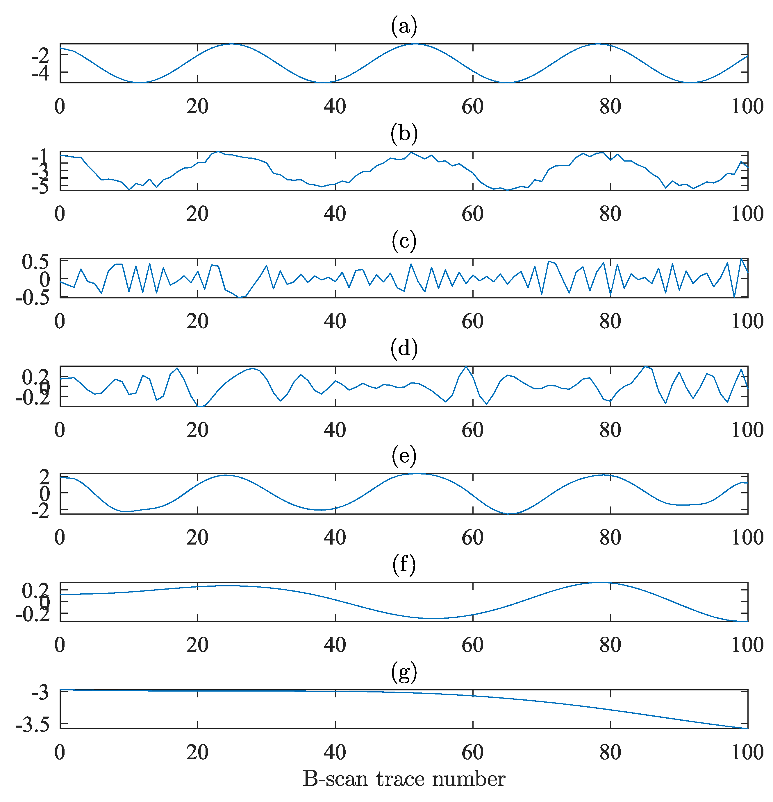
2.1. Dip Filter Based On the f - x EMD

Let $B(t,x)$ denote a GPR B-scan data, which has n traces (i.e., n A-scan). By performing the Fourier transform on each A-scan, the B-scan can be represented in the f - x domain as $B(\omega ,x)$, where $\omega$ is the angular frequency. For each frequency within the frequency bins, the frequency slice can be represented by $B(\omega ,x)$ = [$B(\omega ,x_1)$, $B(\omega ,x_2)$, ..., $B(\omega ,x_n)$]. Its real and imaginary part can be represented apart as $B^{\prime }(\omega ,x)$ and $B^{\prime \prime }(\omega ,x)$, i.e., $B(\omega ,x)=B^{\prime }(\omega ,x)+i{B}^{\prime \prime }(\omega ,x)$.

The f - x EMD is actually an extended application of the classic EMD implemented on the frequency slices in the f - x domain. In the f - x EMD, the real and imaginary part of $B(\omega ,x)$ are decomposed by the EMD, respectively. Considering a certain frequency ${\omega }_m$, the real and imaginary part of the corresponding frequency slice can be decomposed into N IMFs by the EMD respectively, i.e.,

$$B^{\prime }({\omega }_m,x)=\sum _{k=1}^{N}Im{f}_k^{\prime }({\omega }_m,x)+r^{\prime }({\omega }_m,x),$$

(1)

and

$$B^{\prime \prime }({\omega }_m,x)=\sum _{k=1}^{N}Im{f}_k^{\prime \prime }({\omega }_m,x)+r^{\prime \prime }({\omega }_m,x),$$

(2)

where $Im{f}_k^{\prime }({\omega }_m,x)$ denotes the derived kth IMF of real part, $r^{\prime }({\omega }_m,x)$ the monotone residual signal known as the trend term, and $Im{f}_k^{\prime \prime }({\omega }_m,x)$ and $r^{\prime \prime }({\omega }_m,x)$ are the corresponding terms in the imaginary case.

One of the important features of the EMD scheme in f - x domain is that the decomposed IMFs correspond to different wavenumber ranges, and are sorted in the order from high-wavenumber vibrations to low-wavenumber vibrations. So when the first K IMFs of the real and imaginary parts are extracted respectively, the high-wavenumber components ${\acute{B}}_K({\omega }_m,x)$ are adaptively separated from each frequency slice as

$${\acute{B}}_K({\omega }_m,x)=\sum _{k=1}^{K}Im{f}_k^{\prime }({\omega }_m,x)+i\sum _{k=1}^{K}Im{f}_k^{\prime \prime }({\omega }_m,x).$$

(3)

Then the low-wavenumber components ${\overline{B}}_K({\omega }_m,x)$ can be derived by reconstructing the frequency slice from rest of IMFs as follows,

$$\begin{array}{cc}\hfill {\overline{B}}_K({\omega }_m,x)& =B({\omega }_m,x)-{\acute{B}}_K({\omega }_m,x)\hfill \\ \hfill & =B^{\prime }({\omega }_m,x)-\sum _{k=1}^{K}Im{f}_k^{\prime }({\omega }_m,x)+i\left[B^{\prime \prime }({\omega }_m,x)-\sum _{k=1}^{K}Im{f}_k^{\prime \prime }({\omega }_m,x)\right].\hfill \end{array}$$

(4)

By implementing the above f - x EMD among all frequency slices (both the positive and negative frequencies), the high-wavenumber components and low-wavenumber components are primarily separated in the f - x domain, denoted by ${\acute{B}}_K(\omega ,x)$ and ${\overline{B}}_K(\omega ,x)$. When transforming back to t - x domain by the inverse Fourier transform, the corresponding profiles ${\acute{B}}_K(t,x)$ and ${\overline{B}}_K(t,x)$ that features the dipping events and the sub-horizontal layers respectively can be derived.

It should be noted here that the original f - x EMD scheme is designed for denoising, and only the first IMF is removed, i.e., $K=1$. When K takes more than 1, ${\acute{B}}_K(t,x)$ will include more components of relative high wavenumber. We term it as the Kth mode dipping profile, and correspondingly, ${\overline{B}}_K(t,x)$ is termed as Kth mode horizontal profile.

Here, K can be decided from the separated t - x profiles by the interpreter easily, and the maximum of the mode is 3 by some experiments empirically. Some detailed examples are shown in the “Results” section.

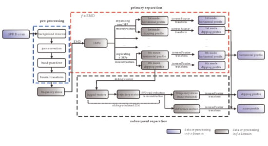
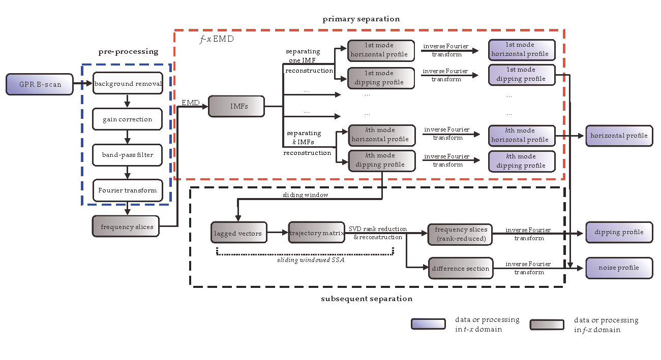
2.2. The Hybrid Approach in f - x Domain

After implementing the dip filter in the former section, most of the dipping events has been extracted in ${\acute{B}}_K(t,x)$, or ${\acute{B}}_K({\omega }_m,x)$ in f - x domain. However, the random noise is still mixed in it. There are several options to further denoise the profile. Here, we select to use the SSA algorithm [19,20] to further separate the dipping reflections and the random noise and then form a hybrid approach in f - x domain.

When the SSA scheme is implemented on a GPR B-scan in f - x domain, each frequency slice is recursively intercepted to a set of lagged vectors as ${[B(\omega ,x_1),B(\omega ,x_2),...B(\omega ,x_{\ell })]}^{\mathrm{T}}$, ${[B(\omega ,x_2),B(\omega ,x_3),...,B(\omega ,x_{\ell +1})]}^{\mathrm{T}}$,...${[B(\omega ,x_{n-\ell +1}),B(\omega ,x_{n-\ell +2}),...,B(\omega ,x_n)]}^{\mathrm{T}}$ so that a Hankel matrix termed as trajectory matrix is formed. Here, ℓ is termed as the embedding dimension for describing the length of these lagged vectors, and in general, it takes the rounded integer of $n/2$. The formulated trajectory matrix is as follows,

$$\mathbf{H}=\left[\begin{array}{cccc}B(\omega ,x_1)& B(\omega ,x_2)& \dots & B(\omega ,x_{n-\ell +1})\\ B(\omega ,x_2)& B(\omega ,x_3)& \dots & B(\omega ,x_{n-\ell +2})\\ ⋮& ⋮& & ⋮\\ B(\omega ,x_{\ell })& B(\omega ,x_{\ell +1})& \dots & B(\omega ,x_n)\end{array}\right].$$

(5)

By using SVD, H can be to decomposed into unitary matrices $\mathbf{U},\mathbf{V}$ and the diagonal matrix $\mathsf{\Sigma }$, i.e., $\mathbf{H}=\mathbf{U}\mathsf{\Sigma }{\mathbf{V}}^H$. If we reduce the reserved rank to r, the singular values of the diagonal of $\mathsf{\Sigma }$ are sorted and only the first r biggest ones remain. Then the rank-reduced trajectory matrix ${\mathbf{H}}_r$ can be recovered by ${\mathbf{H}}_r={\mathbf{U}}_r{\mathsf{\Sigma }}_r{\mathbf{V}}_r^H$, and the updated frequency slice can be derived by averaging its diagonal detailed in the Oropeza’s thesis [20]. The ${\acute{B}}_K(\omega ,x)$ with updated frequency slices in f - x domain can be transformed back to t - x domain ${\acute{B}}_K(t,x)$, and the difference section is classified to the noise section. We remark here due to the reflections along the measurement line by some targets (e.g., small rebars) are discontinuous, the SSA scheme implemented on the whole frequency slices or part of the frequency slices using spatial windows may lose some important dipping events. In this work, the proposed implementation with a sliding window can solve this problem better, and we discuss the comparison of these schemes in the following Result part.

The above processing can be seen as the subsequent separation after the dip filter based on the f - x EMD, and the two parts form the hybrid approach in f - x domain. The corresponding schematic diagram is shown in Figure 1.

3. Results

Three examples are shown in this section. The proposed hybrid approach in f - x domain is tested by using synthetic two-layer model, a simulated data, and field data, respectively.

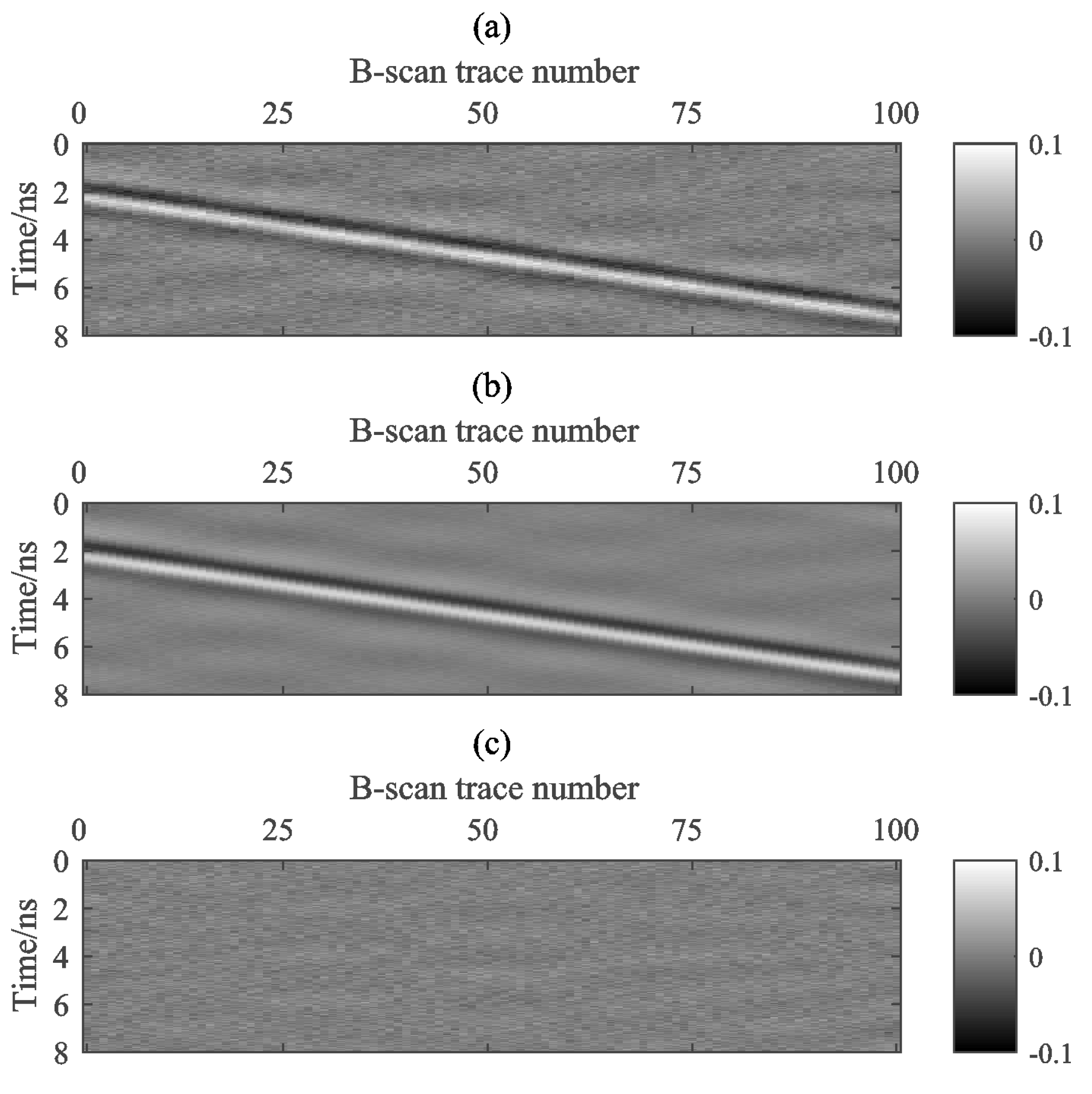
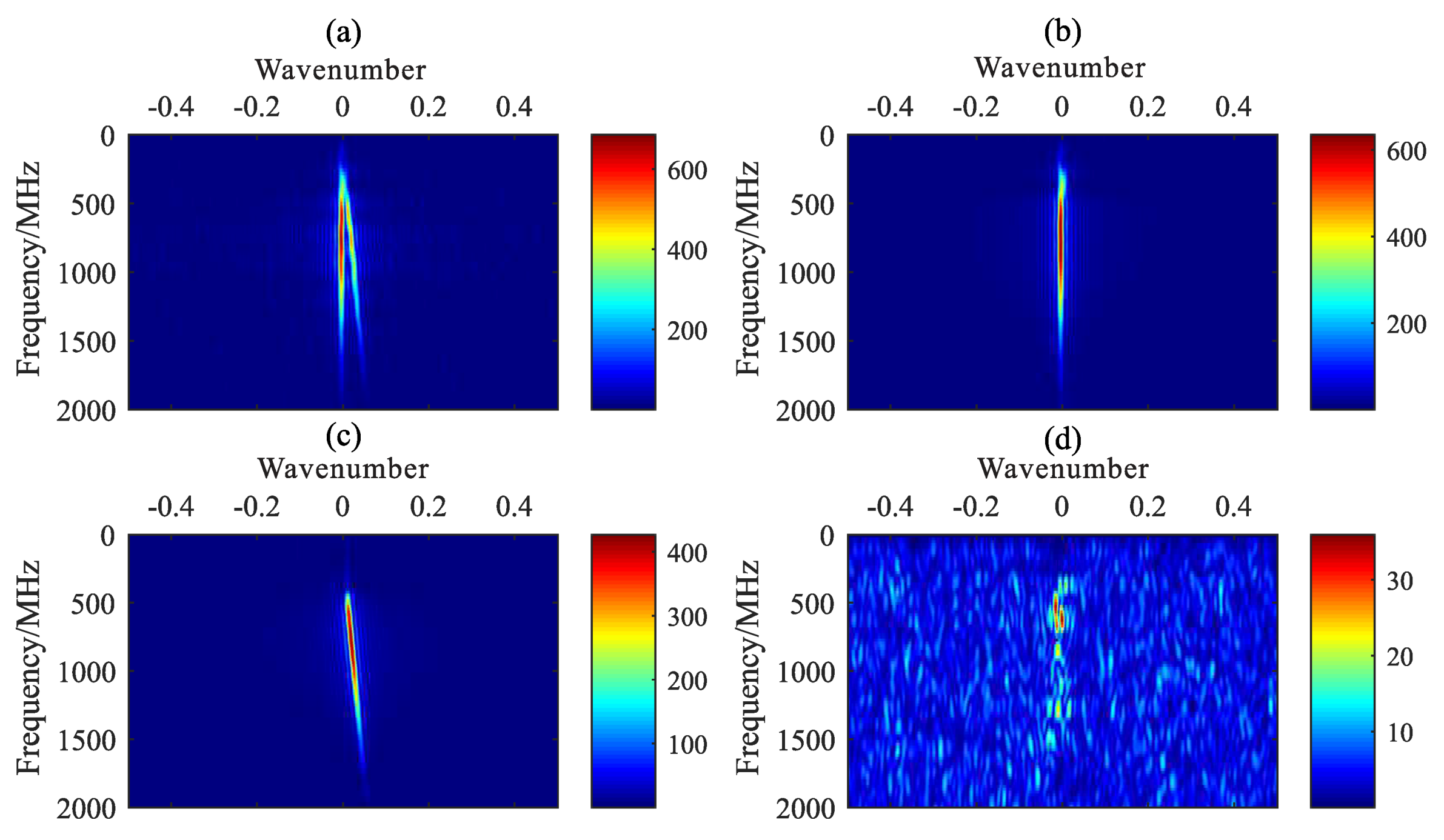
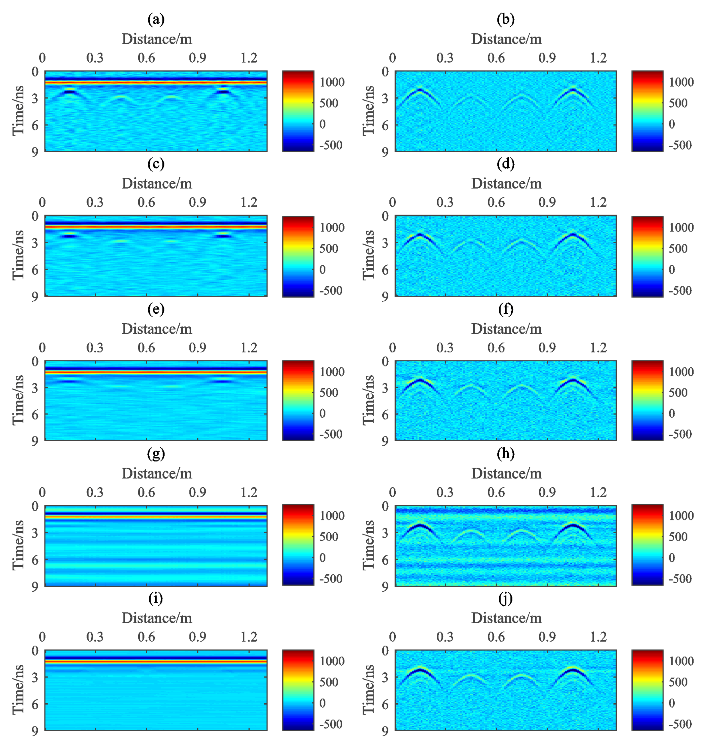
3.1. Synthetic Data Tests

The proposed method is first demonstrated with a synthetic example (Figure 2a), which is simply formulated by the convolution of the two layers and the mixed-phase Ricker wavelet (dominant frequency is 800 MHz). Figure 2 presents the primary separation results of the synthetic B-scan data using the f - x EMD. It is obvious that the shallow layer in this model is horizontal, whereas the deeper one is relatively slant. The corresponding noisy section is shown in Figure 2b, in which the random noise (SNR =10) is added. In the primary separation using the f - x EMD scheme, the dipping events on different levels can be extracted by reconstructing the frequency slices from the first one, two, three and four IMFs in f - x domain respectively, i.e., the 1st - 4th mode dipping profile, and their profiles in t - x domain are shown in Figure 2d,f,h,j. The corresponding sub-horizontal layers can be reconstructed by rest of IMFs of each frequency slice in f - x domain, i.e., the 1st - 4th mode horizontal profile, and their t - x domain profiles are shown in Figure 2c,e,g,i. In the 1st mode profiles (Figure 2c,d), most of the random noise which can be treated as the dipping events at the highest angles is separated. In the 2nd mode profiles, though some dipping structures as well as the artefacts due to strong noise have been extracted in Figure 2f, the dipping layers at low angles are still blended with the horizontal layer, see Figure 2e. Then in the case of removing three IMFs, the horizontal events and the dipping events are well separated into Figure 2g,h respectively, and most of the random noise is contained in Figure 2h as well. When more than three IMFs are removed, some sub-horizontal events which correspond to the relative low wavenumbers are also separated into the dipping profile, and only some horizontal components are left in the horizontal profile. Here we only show the case of K = 4, see Figure 2i,j. Therefore, in this case the K in Equation (3) or (4) takes 3. In contrast, the filtered results by the spatial mean filter (window size is 15 traces) are shown in Figure 2k,l, where the horizontal and dipping events are not separated appropriately.

The above separation process in the f - x EMD scheme can also be revealed by the EMD decomposition implemented on one frequency slice, and here we take the real part of 1200MHz frequency slice for instance in Figure 3. Figure 3a,b are the 1200MHz frequency slices (real part) of the clean and noisy B-scan in f - x domain (see Figure 2a,b), where the noise obviously increases the non-stationarity of the frequency slice. By using the EMD, the frequency slice of the noisy data (i.e., Figure 3b) are decomposed into several IMFs as shown in Figure 3c–g and these derived IMFs are sorted from high-frequency to low-frequency. As more IMFs are separated, more high-frequency components of each frequency slice in f - x domain are extracted and the relatively low-frequency ones remain, so in Figure 2 the dipping and sub-horizontal layers are gradually separated in t-x domain. In the last two IMFs (the 4th and 5th IMFs), there are only several wavenumbers (see Figure 2f,g), and this explains why we have to stop at K = 3 otherwise strong horizontal components will mix in the dipping profiles.

As to the 3rd mode dipping profile section (Figure 2h) which contains both the dipping events and the noise, the subsequent separation needs to be implemented. For comparison, the 3rd dipping profile is copied here in Figure 4a, and Figure 4b,c are the sections after the SSA extraction and the corresponding difference section, respectively. In this example, by using SSA the singular values representing the dipping events are well retrieved in Figure 4b with most of the noise left in Figure 4c. We remark here the SSA can be simply implemented without sliding window in this example, because there are only linear events. By the two-step separation above, the synthetic profile has been separated to three parts, i.e., the 3rd mode horizontal profile (Figure 2g), the 3rd mode dipping profile (Figure 4b) and the noise section (Figure 4c). This can also be observed by their f - k spectrum of the separated sections as shown in Figure 5, where the wavenumber is normalized. Figure 5a is the f - k spectrum of the input noisy GPR data. Figure 5b–d are the f - k spectrum of the horizontal profile, the dipping profile and the random noise, respectively. It is easily observed that the synthetic data can be separated effectively by the proposed hybrid scheme.

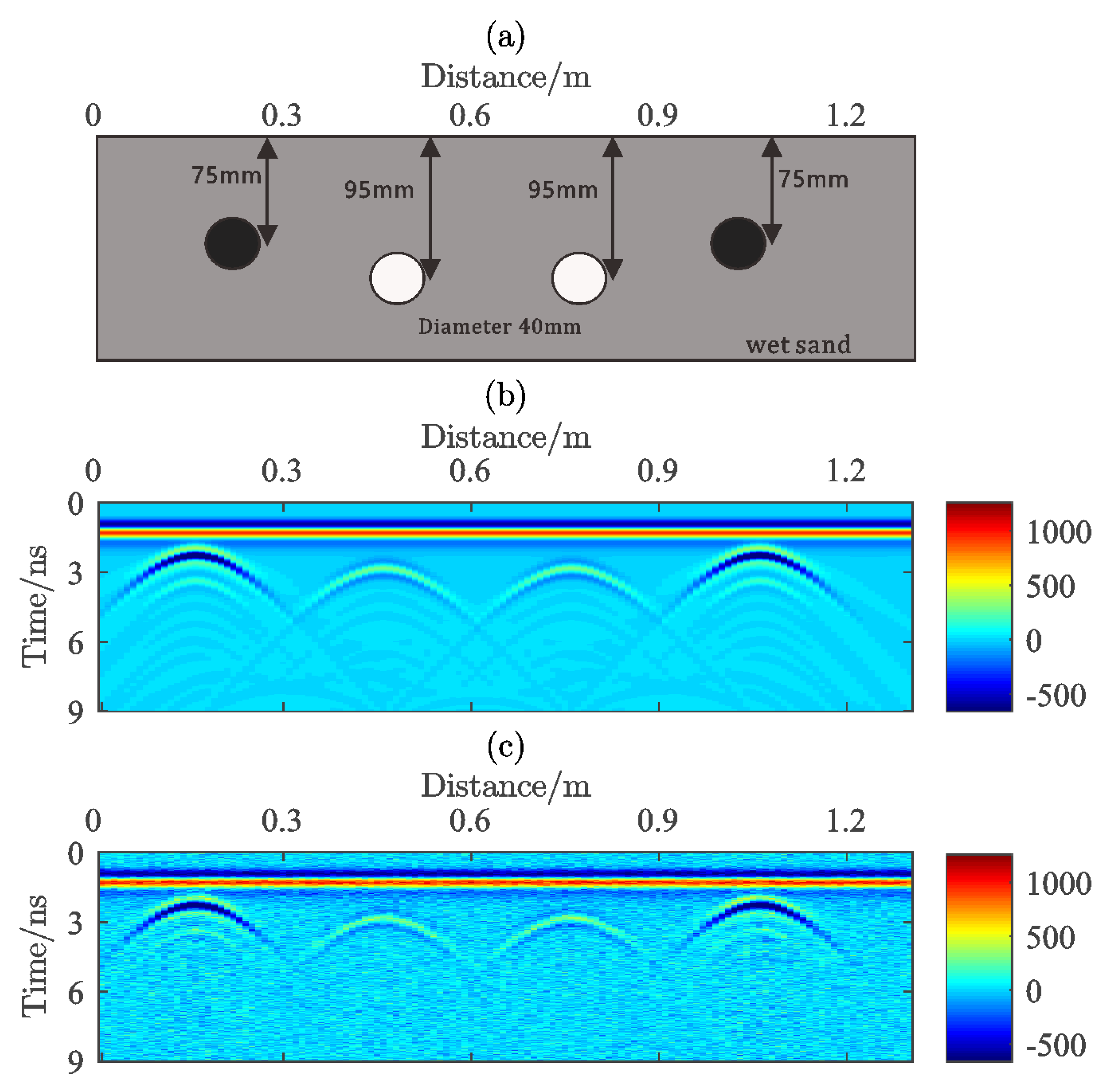
3.2. Forward Simulation Data Tests

In this section, we test the proposed method by the forward simulation data. In the model, there are two different types of cylinder targets in the background of wet sand, i.e., two metal rebars and two hollow tubes, see the schematic drawing in Figure 6a. The metal rebars are denoted by the black circles, and the hollow tubes by the white circles. Their diameters are all 40 mm. Figure 6b is the simulated B-scan by using the open-sourced GPR simulation software gprMax [21,22], and there are a strong direct wave and four hyperbolic diffractions corresponding to the horizontal and dipping features, respectively. The random noise (SNR = 10) is added in Figure 6c, which is used as the test data. Figure 7 shows the primary separation results of the noise-contaminated simulation data, where Figure 7a,c,e,g are the filtering results by removing one, two, three and four IMFs for each frequency slices in the f - x EMD scheme respectively, and the corresponding difference sections are shown on the right (see Figure 7b,d,f,h). It can be easily observed that with more IMFs removed, the hyperbolic diffractions as well as the random noise are gradually separated from the original profile and leave direct wave and some of horizontal parts near the diffraction vertexes behind. When $K=4$ or higher, most of the low-wavenumber components are also separated to the dipping profile, which makes the separated profiles have less geophysical meaning, see Figure 7g,h. In this case, the 3rd mode dip filter (i.e., $K=3$) separates the B-scan better, though there are a few small residuals at the top of the hyperbola diffraction. Here, we also show the separated results using the spatial mean filter (window size = 15 traces) for comparison in Figure 7i,j.

Then we implement the subsequent separation for the noisy dipping profile obtained (see the 3rd mode dipping profile in Figure 7f). In Figure 8, the dipping reflections and the random noise are further separated by implementing the SSA on each frequency slices in f - x domain, where the reserved rank of the SSA scheme and different types of window are discussed. Figure 8a,c are both the dipping events processed by the f - x SSA without applying any local windows, where the reserved rank of SSA is 3 and 5 respectively, and their corresponding residual difference sections are shown in Figure 8b,d. It is obvious that the subsequent separation effect is not ideal for the dipping hyperbola diffractions when the SSA are implemented on each frequency slices without any windows, because some important dipping events are left in the noise sections. Figure 8e is the separated dipping profile by the f - x SSA (rank = 3) with spatial windows (window size = 15 traces, overlapping 6 traces), and the Figure 8g is that by the f - x SSA (rank = 3) with sliding windows (window size = 15 traces). The corresponding residual difference sections treated as noise are shown in the right column, i.e., Figure 8f,h. In this case, the subsequent separation by SSA with sliding windows achieves better results.

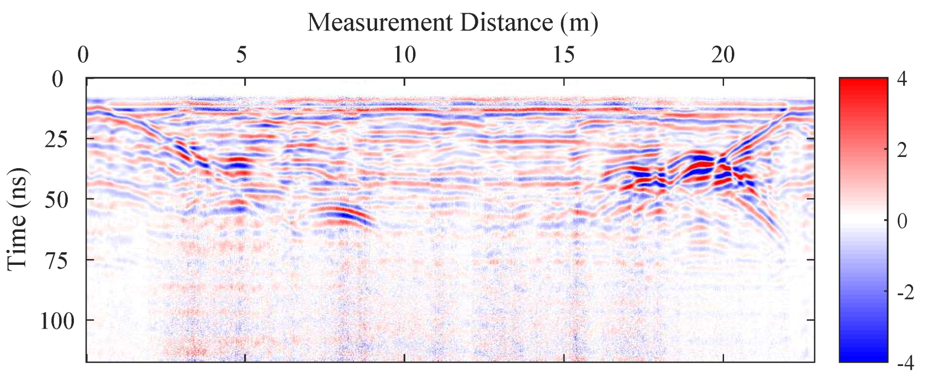
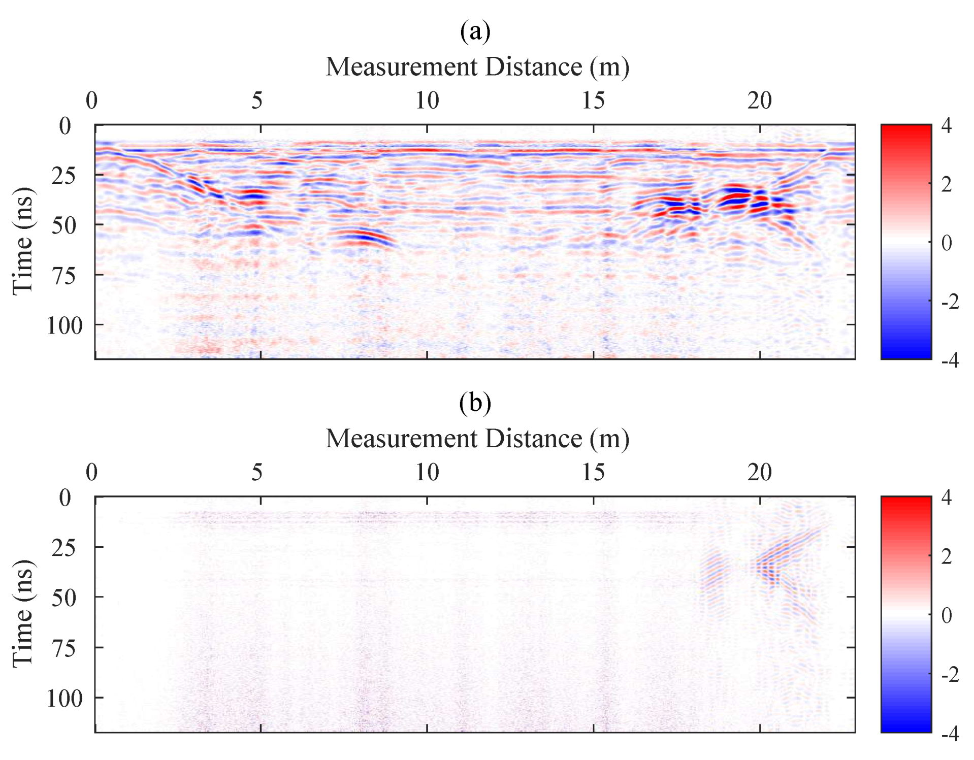
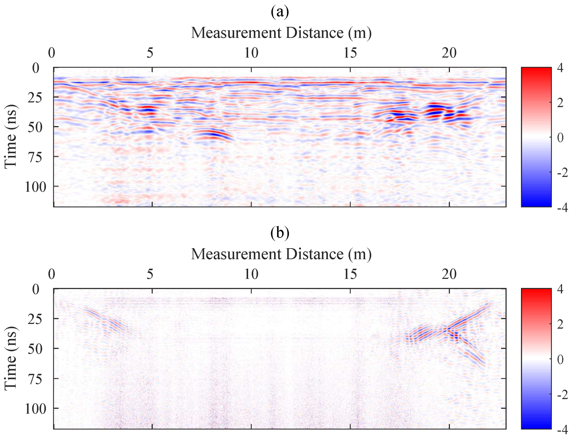
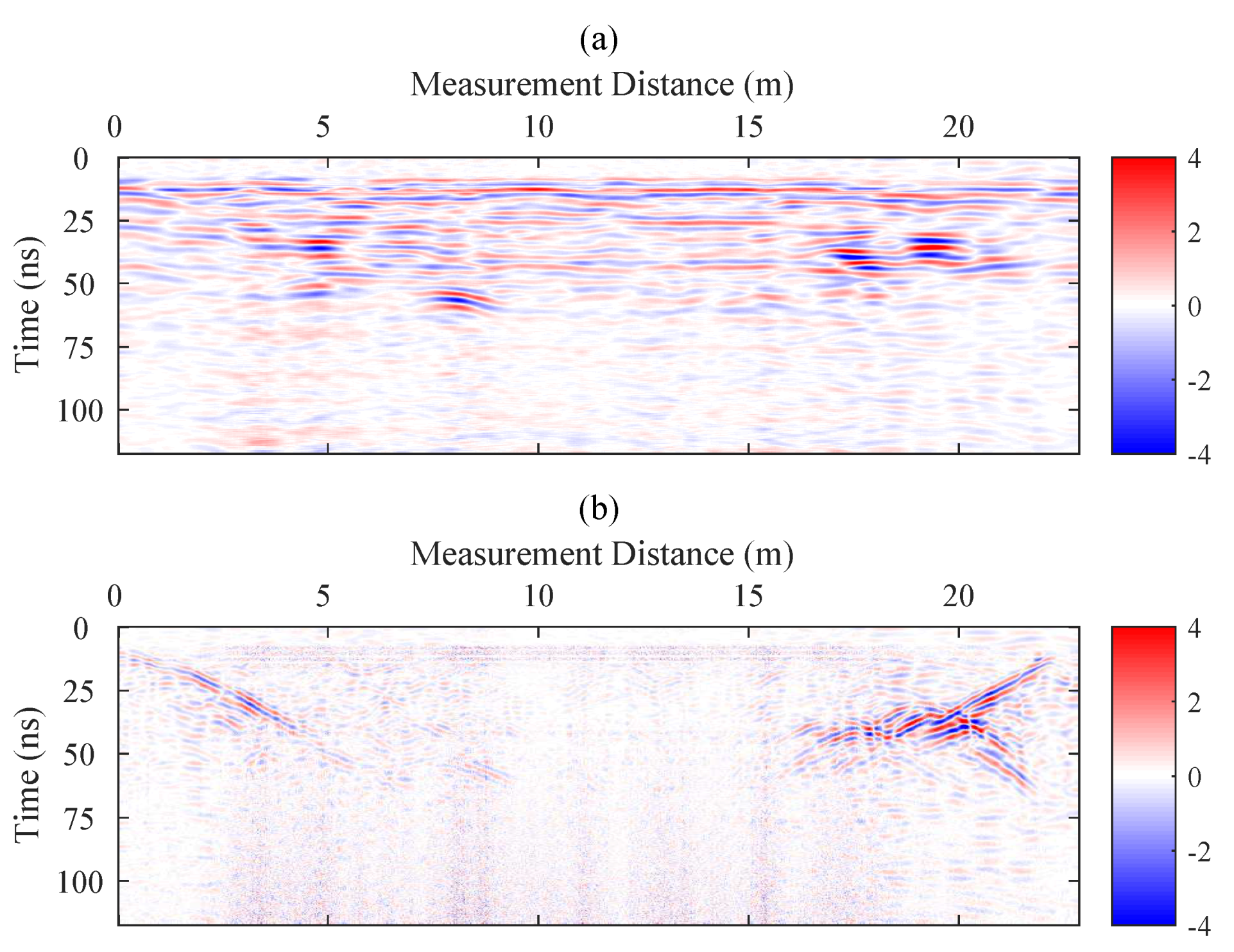
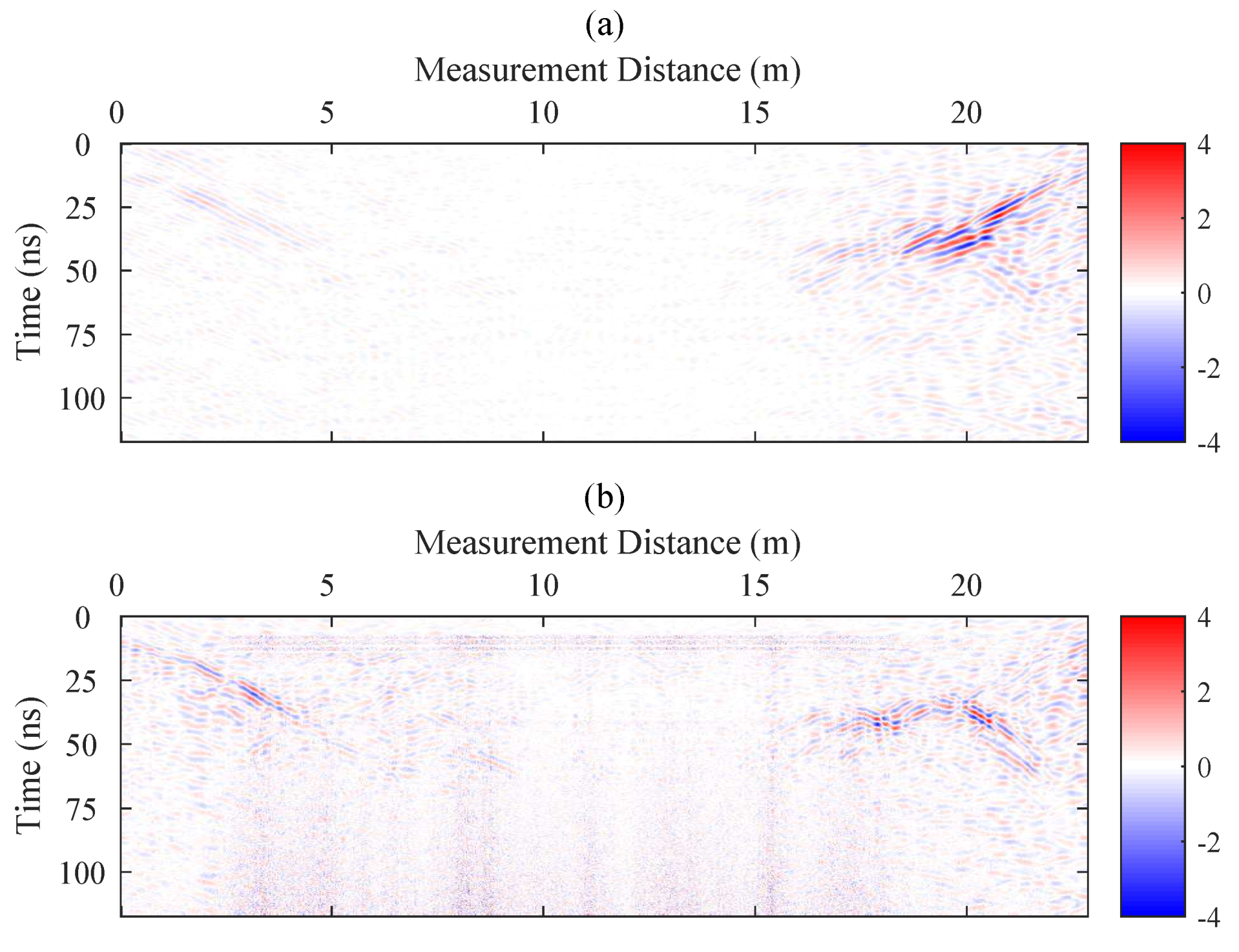
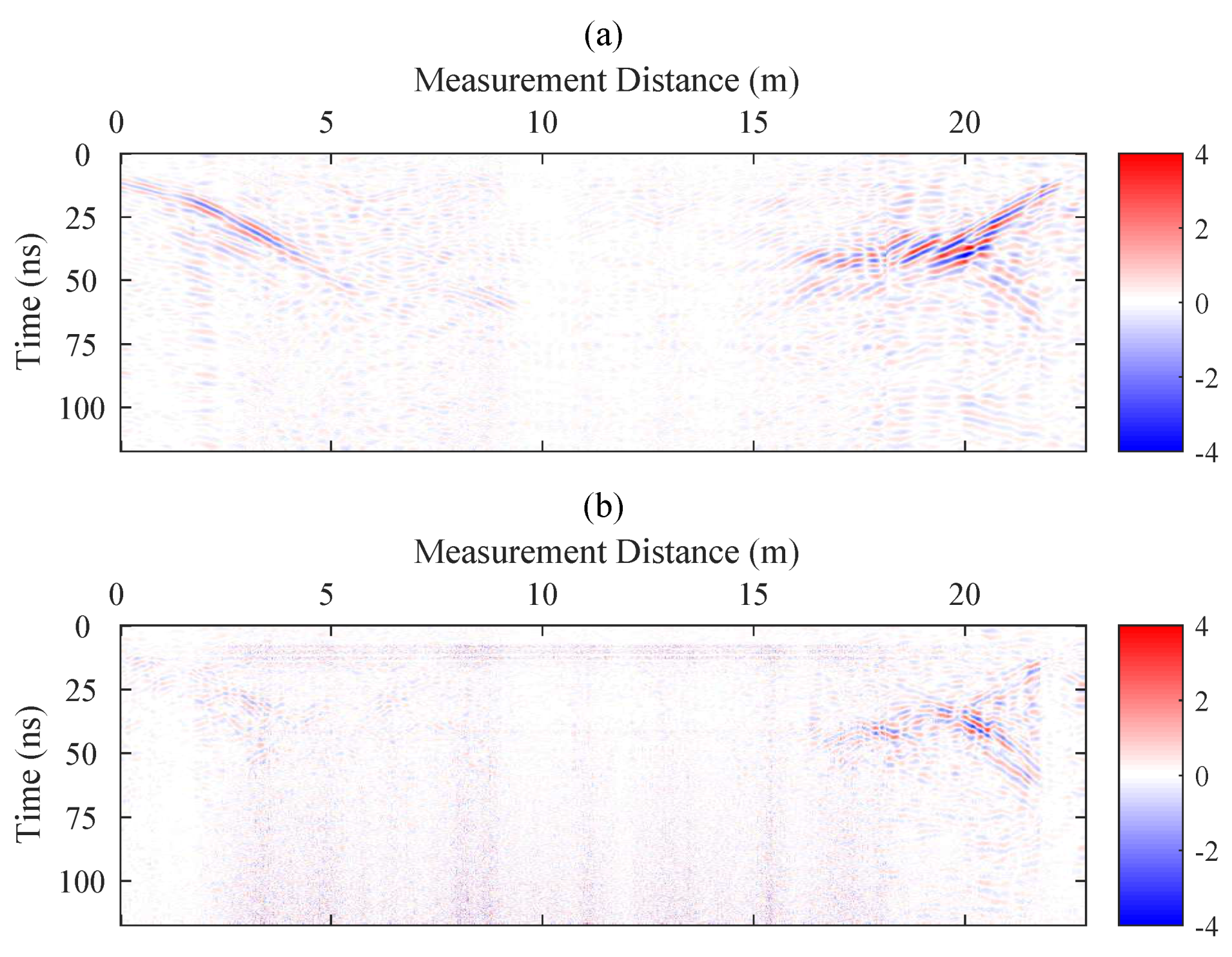
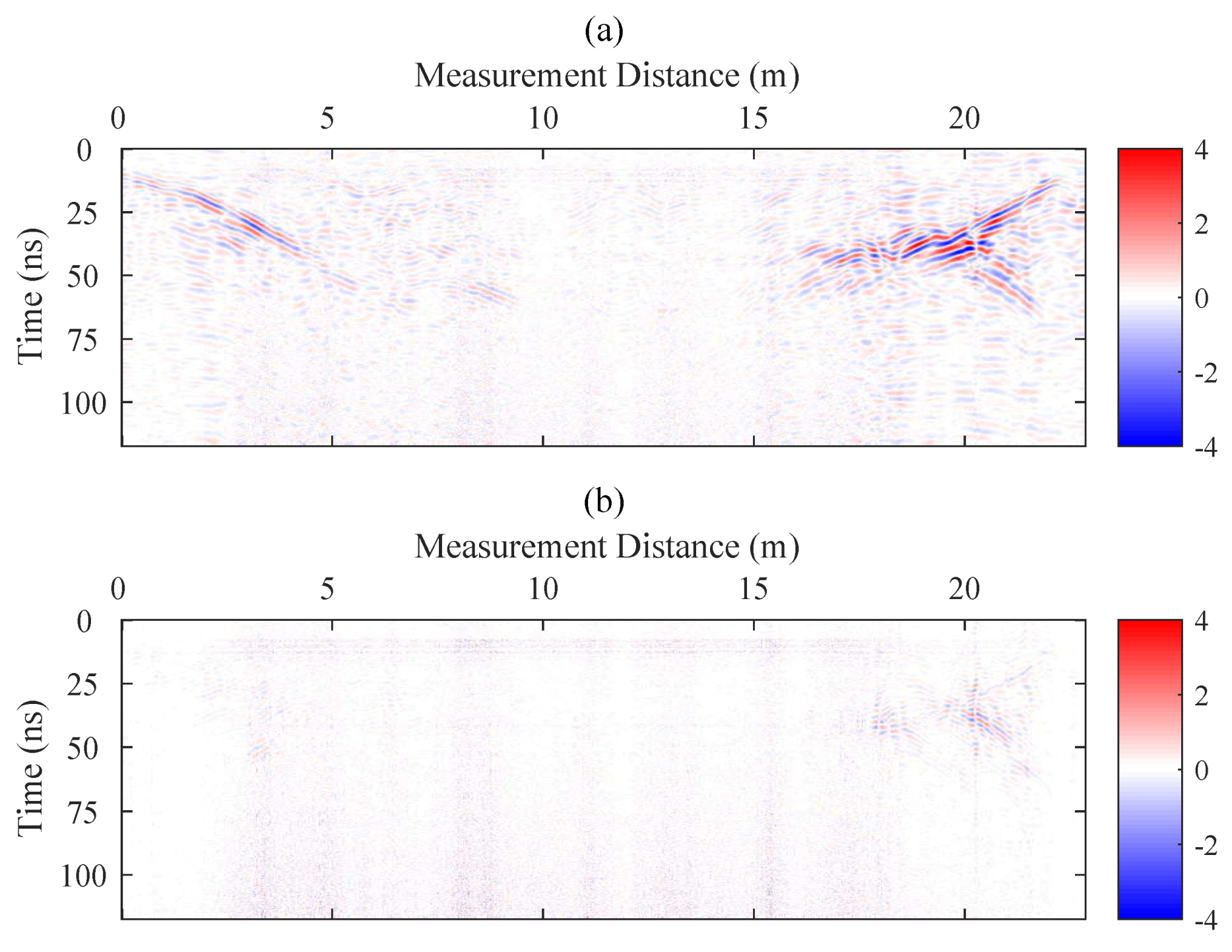
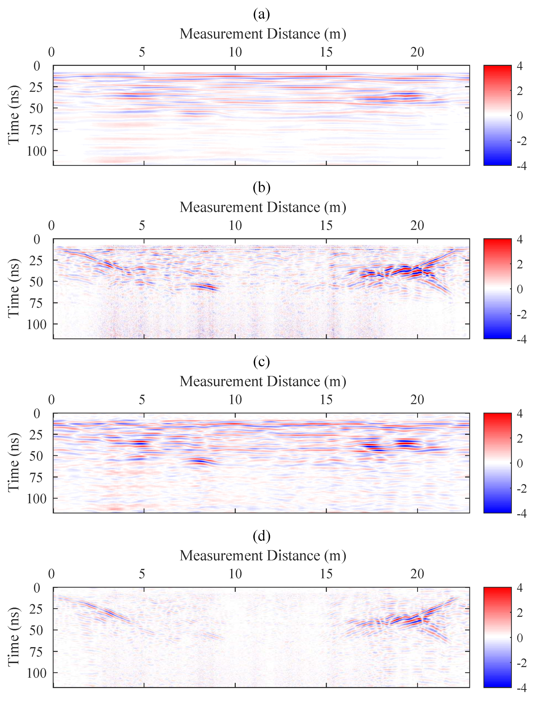
3.3. Field Data Results

In this section, we apply the proposed method to the field GPR data shown in Figure 9, which is collected by the 250 MHz shielded antenna of the MALÅ system at the IFSTTAR Geophysical Test Site, France [23]. The time-window length of the dataset is about 117 ns and the measurement distance about 23 m. There are dipping embankments and the embedded objects between them.

The primary separation results of the field GPR data using the f - x EMD are shown in Figure 10, Figure 11 and Figure 12, in which the horizontal profiles of different mode are presented by (a) and the dipping profiles of different mode are presented by (b). In Figure 10 and Figure 11, the dipping events such as the two dipping embankments are not evident, and the lateral discontinuity still exists in the horizontal profiles. However, the sub-horizontal layers in the 3rd mode horizontal profiles are more continuous (see Figure 12a), and meanwhile, the dipping embankments and some hyperbolic diffractions as well as most of the noise are all separated to the 3rd mode dipping profile (Figure 12b). In addition, when more than three IMFs are removed from each frequency slices, some sub-horizontal layers are also separated to the dipping profile, which is not beneficial to the interpretation work, though they are not shown in the test. $K=3$ in this case is appropriate.

Then we process the noisy dipping profile obtained (Figure 12b) by implementing the subsequent separation (i.e., denoising). Figure 13, Figure 14 and Figure 15 are the dipping reflections separated by SSA using the different window schemes and the corresponding difference sections. The separated results using SSA without any window and spatial windows (window size = 25 traces, overlapping 6 traces) are shown in Figure 13a and Figure 14a respectively, however, there are still some dipping events left in the corresponding difference sections (see Figure 13b and Figure 14b). In contrast, Figure 15a shows the separated results using SSA with the sliding windows (window size = 25 traces), where most of the dipping events remain, and the random noise is moved to the corresponding difference section as shown in Figure 15b.

Figure 16 shows the final separation results by the proposed scheme, see Figure 16c,d, and the separated results using the spatial mean filter (window size = 25 traces) in Figure 16a,b are also shown here for comparison. The profile shown in Figure 16c that features the sub-horizontal layers is in fact the 3rd horizontal profile after the primary separation step. Figure 16d is the dipping profiles through the two-step separation step including the dip filter and the subsequent denoising. The dipping features (see the dipping embankments) in the dipping profile using the proposed scheme are clearer and less affected by noise. Meanwhile, the horizontal features are more continuous.

4. Discussion

We have shown three examples of the proposed hybrid scheme, and we will discuss its benefits and limitations in this section.

The feasibility of the proposed dip filter relies on the adaptivity and sparsity of the EMD decomposition in f - x domain. The main advantage of the proposed hybrid scheme is the semi-adaptive way of decomposing GPR B-scans into pairs of profiles highlighting the sub-horizontal and dipping components separately and its intuitive procedures of setting parameters. Compared to the other existing dip filters, there is only one parameter to be determined in the proposed scheme, i.e., the profile mode, which can be intuitively judged from only a few separated profiles. This just avoids the difficulties of selecting thresholds for wavelet coefficients or adjusting filter parameters artificially, which require interpreters to have good mathematical basis. Then most of the random noise can also be further separated, and the sub-horizontal and dipping components of GPR B-scans can be highlighted without noise interference.

However, both the horizontal and the dipping components are vital for the interpretation, and some diffractions may be separated to the different profiles by using the proposed scheme. For instance the horizontal parts near the vertex and the dipping parts along the arms which both contribute to the interpretation of the subsurface targets are separated (see the forward simulation example in Section 3.2), so we remark that the separated profiles should be cross-referenced, and the proposed method can also be implemented after the migration with an accurate velocity. In the future work, we will introduce some more intelligent algorithms (e.g., machine learning) to make the procedures of parameter selection more adaptive, and some algorithms such as automatic event picking or fault recognition can also be applied to the separated profiles.

5. Conclusions

The proposed hybrid scheme in f - x domain mainly consists of two parts, i.e., the adaptive dip filter derived from the f - x EMD and the denoising by SSA with sliding windows. It can separate the sub-horizontal layers and the dipping structures or events as well as the random noise properly. By using the proposed scheme, the structures at different dips in GPR B-scans can be revealed more clearly, and more different aspects can be provided in the interpretation work.

The effectiveness of this work has been illustrated by three examples. Though the proposed hybrid scheme can realize the separation almost adaptively, there are still some parts need to be decided by observing the intermediate results, such as the mode of the separated profile and the remaining rank. We wish to further improve the scheme by bonding some intelligent algorithms in the future so that the scheme can separate the GPR B-scans more adaptively and more in line with the needs of the interpretation work.

References

1. Benedetto, A.; Tosti, F.; Bianchini Ciampoli, L.; D’Amico, F. An Overview of Ground-Penetrating Radar Signal Processing Techniques for Road Inspections. Signal Process. 2017, 132, 201–209. [Google Scholar] [CrossRef]
2. Solla, M.; Lagüela, S. Editorial for Special Issue “Recent Advances in GPR Imaging”. Remote Sens. 2018, 10, 676. [Google Scholar] [CrossRef]
3. Tzanis, A. Detection and Extraction of Orientation-and-Scale-Dependent Information from Two-Dimensional GPR Data with Tuneable Directional Wavelet Filters. J. Appl. Geophys. 2013, 89, 48–67. [Google Scholar] [CrossRef]
4. Tzanis, A. MatGPR Release 2: A Freeware Matlab® Package for the Analysis and Interpretation of Common and Single Offset GPR Data. FastTimes 2010, 15, 17–43. [Google Scholar]
5. Tzanis, A.; Kafetsis, G. A Freeware Package for the Analysis and Interpretation of Common-Offset Ground Probing Radar Data, Based on General Purpose Computing Engines. Bull. Geol. Soc. Greece 2004, 36, 1347–1354. [Google Scholar] [CrossRef]
6. Davies, E. Machine Vision: Theory, Algorithms and Practicalities; Academic Press: Waltham, MA, USA, 1990; pp. 51–60. [Google Scholar]
7. Spitz, S. Seismic Trace Interpolation in the F-X Domain. Geophysics 1991, 56, 785–794. [Google Scholar] [CrossRef]
8. Hornbostel, S. Spatial Prediction Filtering in the t-x and f-x Domains. Geophysics 1991, 56, 2019–2026. [Google Scholar] [CrossRef]
9. Nuzzo, L.; Quarta, T. Improvement in GPR Coherent Noise Attenuation Using τ-p and Wavelet Transforms. Geophysics 2004, 69, 789–802. [Google Scholar] [CrossRef]
10. Herrmann, F.; Wang, D.; Hennenfent, G.; Moghaddam, P. Curvelet-Based Seismic Data Processing: A Multiscale and Nonlinear Approach. Geophysics 2008, 73. [Google Scholar] [CrossRef]
11. Terrasse, G.; Nicolas, J.; Trouvé, E.; Drouet, É. Application of the Curvelet Transform for Clutter and Noise Removal in GPR Data. IEEE J. Sel. Top. Appl. Earth Obs. Remote Sens. 2017, 10, 4280–4294. [Google Scholar] [CrossRef]
12. Wang, X.; Liu, S. Noise Suppressing and Direct Wave Arrivals Removal in GPR Data Based on Shearlet Transform. Signal Process. 2017, 132, 227–242. [Google Scholar] [CrossRef]
13. Bekara, M.; van der Baan, M. Random and Coherent Noise Attenuation by Empirical Mode Decomposition. Geophysics 2009, 74, V89–V98. [Google Scholar] [CrossRef]
14. Huang, N.E.; Shen, Z.; Long, S.R.; Wu, M.C.; Shih, H.H.; Zheng, Q.; Yen, N.-C.; Tung, C.C.; Liu, H.H. The Empirical Mode Decomposition and the Hilbert Spectrum for Nonlinear and Non-Stationary Time Series Analysis. Proc. R. Soc. Lond. A 1998, 454, 903–995. [Google Scholar] [CrossRef]
15. Chen, Y.; Ma, J. Random Noise Attenuation by f-x Empirical-Mode Decomposition Predictive Filtering. Geophysics 2014, 79, V81–V91. [Google Scholar] [CrossRef]
16. Chen, Y.; Gan, S.; Liu, T.; Yuan, J.; Zhang, Y.; Jin, Z. Random Noise Attenuation by a Selective Hybrid Approach Using f-x Empirical Mode Decomposition. J. Geophys. Eng. 2015, 12, 12. [Google Scholar] [CrossRef]
17. Cagnoli, B.; Ulrych, T.J. Singular Value Decomposition and Wavy Reflections in Ground-Penetrating Radar Images of Base Surge Deposits. J. Appl. Geophys. 2001, 48, 175–182. [Google Scholar] [CrossRef]
18. Zhang, X.; Nilot, E.; Feng, X.; Ren, Q.; Zhang, Z. Imf-Slices for Gpr Data Processing Using Variational Mode Decomposition Method. Remote Sens. 2018, 10, 476. [Google Scholar] [CrossRef]
19. Oropeza, V.; Sacchi, M. Simultaneous Seismic Data Denoising and Reconstruction Via Multichannel Singular Spectrum Analysis. Geophysics 2011, 76, V25–V32. [Google Scholar] [CrossRef]
20. Elsner, J.B.; Tsonis, A.A. Singular Spectrum Analysis: A New Tool in Time Series Analysis; Springer: Boston, MA, USA, 1996; pp. 39–50. [Google Scholar]
21. Giannakis, I.; Giannopoulos, A.; Warren, C. A Realistic Fdtd Numerical Modeling Framework of Ground Penetrating Radar for Landmine Detection. IEEE J. Sel. Top. Appl. Earth Obs. Remote Sens. 2016, 9, 37–51. [Google Scholar] [CrossRef]
22. Warren, C.; Giannopoulos, A.; Giannakis, I. Gprmax: Open Source Software to Simulate Electromagnetic Wave Propagation for Ground Penetrating Radar. Comput. Phys. Commun. 2016, 209, 163–170. [Google Scholar] [CrossRef]
23. Dérobert, X.; Pajewski, L. TU1208 Open Database of Radargrams: The Dataset of the IFSTTAR Geophysical Test Site. Remote Sens. 2018, 10, 530. [Google Scholar] [CrossRef]
Figure 1. Schematic diagram of the proposed hybrid approach in f - x domain.
Remotesensing 11 02180 g001
Figure 2. (a) Synthetic B-scan data. (b) The B-scan section with the random noise (SNR = 10). (c,e,g,i) are the 1st, 2nd, 3rd and 4th mode horizontal profile after the primary separation of (b) respectively, and (d,f,h,j) are the corresponding dipping profile. In the 3rd mode profiles, the sub-horizontal layers and the dipping events are well separated into (g,h) respectively, and most of random noise is contained in (h) as well. In contrast, the separated results by using the spatial mean filter are shown in (k,l).
Remotesensing 11 02180 g002
Figure 3. Demonstration of the f - x EMD scheme (take one frequency slice as an example). (a,b) are the 1200 MHz frequency slices (real part) of the clean and noisy B-scan (in Figure 2a,b) in f - x domain, where the noise obviously increase the non-stationarity of the frequency slices. (cg) are the decomposed IMFs of the frequency slice of the noisy data (i.e., Figure 3b) by using the EMD decomposition.
Remotesensing 11 02180 g003
Figure 4. The dipping events and the random noise are subsequently separated by using the SSA in f - x domain. (a) The section which contains both the dipping events and the noise, which is same as Figure 2f. (b,c) are the section after the SSA extraction and the corresponding difference section, respectively. In this example, by using SSA the singular values representing the dipping events are well retrieved in (b) with most of the noise left in (c).
Remotesensing 11 02180 g004
Figure 5. The f - k spectrum of the sections separated by the proposed hybrid scheme. (a) the f - k spectrum of the input noisy GPR data. (bd) are the f - k spectrum of the horizonal profile, the dipping profile and the random noise, respectively.
Remotesensing 11 02180 g005
Figure 6. (a) The sketch map of the 2D forward simulation model, where two types of cylinder target in the background of wet sand, i.e., two metal rebars ( ϕ 40mm, in blank) and two hollow tubes ( ϕ 40 mm, in white). (b,c) are the simulated GPR B-scans without and with the random noise (SNR = 10) respectively.
Remotesensing 11 02180 g006
Figure 7. The primary separation results of the noise-contaminated simulation data. (a,c,e,g) are the 1st, 2nd, 3rd and 4th mode horizontal profile after the primary separation respectively, and (b,d,f,h) are the corresponding dipping profile. (i,j) are the separated results using the spatial mean filter (window size = 15 traces) for comparison.
Remotesensing 11 02180 g007
Figure 8. The subsequent separation of dipping events and noise using the SSA in f - x domain. (a) the extracted dipping events by the f - x SSA (rank = 3) without local windows and (b) the residual section; (c) the extracted dipping events by the f - x SSA (rank = 5), without local windows and (d) the residual section; (e) the extracted dipping events by the f - x SSA (rank = 3), with spatial windows (window size = 15 traces, overlapping 6 traces) and (f) the residual section; (g) the extracted dipping events by the f - x SSA (rank = 3) with sliding windows (window size = 15 traces) and (h) the residual section.
Remotesensing 11 02180 g008
Figure 9. Field GPR B-scan.
Remotesensing 11 02180 g009
Figure 10. The 1st mode horizontal profile (a) and dipping profile (b) of the primary separation.
Remotesensing 11 02180 g010
Figure 11. The 2nd mode horizontal profile (a) and dipping profile (b) of the primary separation.
Remotesensing 11 02180 g011
Figure 12. The 3rd mode horizontal profile (a) and dipping profile (b) of the primary separation.
Remotesensing 11 02180 g012
Figure 13. The subsequent separation of dipping events and noise using the SSA without window in the f - x domain (a) and the corresponding difference section (b).
Remotesensing 11 02180 g013
Figure 14. The subsequent separation of dipping events and noise using the SSA with overlapping windows in the f - x domain (a) and the corresponding difference section (b).
Remotesensing 11 02180 g014
Figure 15. The subsequent separation of dipping events and noise using the SSA with sliding windows in the f - x domain (a) and the corresponding difference section (b).
Remotesensing 11 02180 g015
Figure 16. The final separation results by the proposed scheme. The horizontal profile (a) and the dipping profile (b) separated by using the spatial mean filter (window size = 25 traces); The horizontal profile (c) and the dipping profile (d) finally separated by the proposed scheme in f - x domain.
Remotesensing 11 02180 g016