Automatic Methodology to Detect the Coastline from Landsat Images with a New Water Index Assessed on Three Different Spanish Mediterranean Deltas

Abstract

Due to the importance of coastline detection in coastal studies, different methods have been developed in recent decades in accordance with the evolution of measuring techniques such as remote sensing. This work proposes an automatic methodology with new water indexes to detect the coastline from different multispectral Landsat images; the methodology is applied to three Spanish deltas in the Mediterranean Sea. The new water indexes use surface reflectance rather than top-of-atmosphere reflectance from blue and shortwave infrared (SWIR 2) Landsat bands. A total of 621 sets of images were analyzed from three different Landsat sensors with a moderate spatial resolution of 30 m. Our proposal, which was compared to the most commonly used water indexes, showed outstanding performance in automatic detection of the coastline in 96% of the data analyzed, which also reached the minimum value of bias of $-0.91$ m and a standard deviation ranging from ±4.7 and ±7.29 m in some cases in contrast to the existing values. Bicubic interpolation was evaluated for a simple sub-pixel analysis to assess its capability in improving the accuracy of coastline extraction. Our methodology represents a step forward in automatic coastline detection that can be applied to micro-tidal coastal sites with different land covers using many multi-sensor satellite images.

1. Introduction

The coastal areas constitute one of the most productive yet vulnerable ecosystems in the world [1]. Furthermore, most of the world population is concentrated in the coastal area, with up to 60% living close to the sea [2,3]. As a consequence, coastline monitoring must be an essential issue for public policies regarding coastal management.

The coastal zone is a very dynamic environment affected by different factors, such as hydrography, geology, climate, and vegetation [4]. The increasing development of coastal areas causes persistent erosion and flooding problems [5]. Therefore, the knowledge and assessment of the shifts in shoreline position are crucial in the understanding of the morphodynamic processes driving changes [6]. Thus, coastal observation is under permanent development to improve measuring capabilities and to characterize processes related to water quality, hydrodynamics, meteorology, and ecology, as well as submarine geomophology [7].

During the last decades, the most commonly used methods for coastline mapping were field surveys [8,9] and aerial photography [10,11]. Although aerial photographs provide good spatial coverage of the coast [12], temporal coverage can be restricted [13]. To avoid such limitations, remote sensing techniques constitute a good alternative due to the increase in the availability of satellite images; the improvement in spatial, temporal, and radiometric resolution on satellite sensors; and the development of tools for geographic data analysis (Geographic Information Systems (GIS)) as well as of image processing techniques [14]. During the last 30 years, images from different types of satellites have been used to detect coastline, such as radar images, e.g., Synthetic Aperture Radar (SAR) from European Remote Sensing satellite (ERS-1) [15] and ERS-2 [16], high spatial resolution (between 0.5 m and 2.5 m) in multispectral images from DubaiSat-1 and DubaiSat-2 satellites [17], WorldView-2 satellite images [18], and moderate spatial resolution in multispectral images (Operational Land Imager) from satellite Landsat 8 [19].

The Landsat project is one of the most frequently used sources of space-based imagery for Earth studies due to the large collection of multispectral imaging of moderate spatial and temporal resolution; in addition, it is a free access database since 2008 [20]. Therefore, it has been widely used in different areas such as agriculture [21], forestry [22,23], disaster prevention [24], hydrology [25], land planning [26,27], etc. Nowadays, there are two satellites still in orbit, Landsat 7 and Landsat 8.

Many researchers such as Zhu [28], Rasuly et al. [29], Zhang et al. [30], and Rokni et al. [31] have been using Landsat images to detect and monitor the coastline using visible and infrared multispectral bands. Although the Landsat project allows to develop long-term (between 10 and 30 years) analyses due to the large image collection [29,32,33], an important limitation in some cases is the spatial resolution. Landsat images permit a coarse pixel analysis, which in some cases is not detailed enough to detect small or sub-pixel features or changes [34]. In these circumstances, a sub-pixel methodology by super resolution techniques may be useful [35], such as interpolation techniques [36,37]. Most of the accepted interpolation methods for image spatial resolution improvement are based on nearest neighbor and bilinear and bicubic interpolation [38,39,40].

Different types of image processing techniques have been developed for coastline detection, such as segmentation and single band threshold [41,42]; segmentation based on local spectral histogram and level set method [43], which is based on active contours or snakes [44,45]; water indexes [46,47]; classification techniques such as neural network, isodata, support vector machine among others [48,49,50]; fuzzy logic [51]; band ratio [52]; high water-line visual interpretation [53,54,55,56]; and edge detection [57]. Some of these techniques are made by manual detection [43], and others allow an automatic image processing, which is often required in cases like classification of surface water to mask water pixels and in enabling effective monitoring [58]. This is essential when long-term studies are conducted because automating the process reduces human errors since it requires minimal or no human intervention and improves the standardization and efficiency of the studies.

Deltas are among the most environmentally dynamic ecosystems in the world [59]. They are also one the most affected coastal environments due to natural resources and human influence [60]. The deltaic coastal areas are used nowadays as human settlements and for different activities such as tourism, natural reserves, and agriculture, among other things, making this area of high ecological, economic, and social importance [61]. Hence, one of the main concerns of these areas is related to the impact of the sea level rise driven by climate change [62], which results, among other things, in coastline retreat. For this reason, it is essential to track coastline changes to understand the relationship between spatiotemporal patterns of sea-level rise and those of coastline changes which requires studying the coastline dynamic at large spatial scales and over long time periods [63].

It is clear that long-term studies are necessary to better understand coastal changes, so automated methodologies are essential to carry out this task. Also, in some cases, the unsupervised classification methods are useful due to their flexibility [64] where there is no need to feed the algorithm with prior ground information [65], which is time consuming and can induce higher human errors. The proposed water indexes combined with the methodology followed gave outstanding results in coastline detection from different sites with different land covers. Also, it showed the effectiveness in detecting a greater quantity of shorelines from different Landsat sensors in different coastal areas compared to the usual indexes used over all the images analyzed in this paper, with a high positional accuracy in the coastlines detected. The methodology proposed has the advantage to be simple, with relatively high accuracy and low-cost implementation.

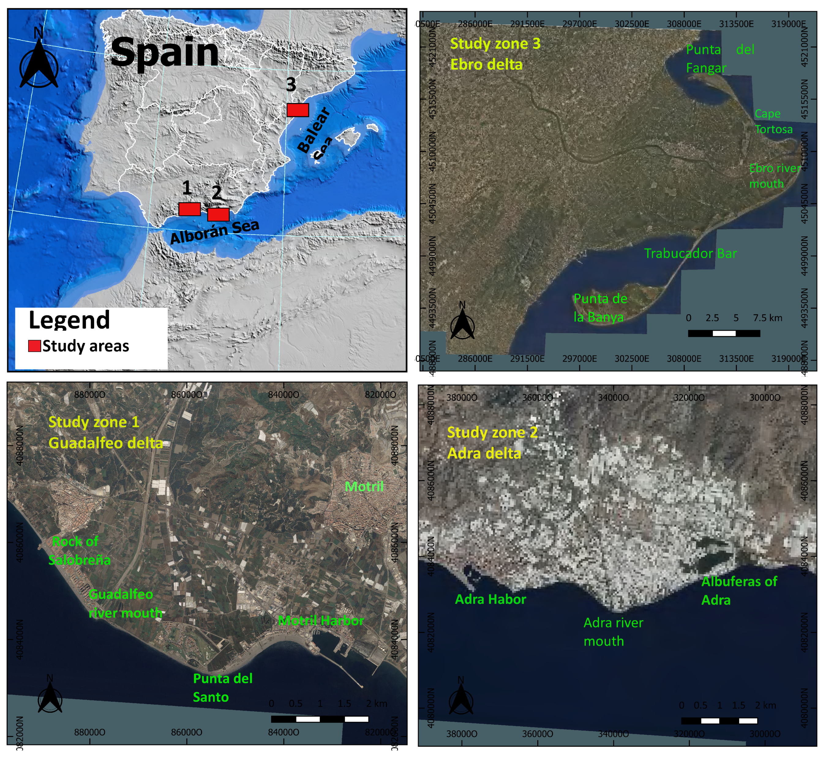
This research proposes a methodology to automatically extract the coastline from different satellite images by the combination of different processing techniques commonly used in the literature. The methodology includes a new water spectral index, which improves the effectiveness to detect the coastline compared to three of the existing and most common water indexes used: the modified normalized difference water index (MNDWI), the normalized water index (NDWI), and the automated water extraction index (AWEI). The methodology was applied to different deltas located on the Spanish Medierranean coast (Guadalfeo, Adra, and Ebro). Multispectral satellite images from three different sensor, i.e., the thematic mapper (TM), the enhanced thematic mapper plus (ETM+), and the operational land imager (OLI) of the Landsat project were used, which increased their spatial resolution by bicubic interpolation in order to asses a simple sub-pixel analysis. Accuracy assessment was done by comparing the coastline extracted to high resolution data.

2. Study Sites

Three different river deltas (Figure 1) were selected in this study to apply the new methodology and to compare the water-index behavior. An important characteristic that influenced the selection of the three study zones is their micro-tidal conditions (a tidal range of approximately 0.5 m in the Guadalfeo, usually not exceeding 1.0 m high in the Adra delta [61], and a maximum tidal range about of 0.25 m in the Ebro delta [66]). This research aims to detect automatically the coastline from sites with different land use using a water spectral index, the delta morphologic analysis is out of the scope of this paper.

2.1. Guadalfeo River Delta

The Guadalfeo river catchment has an area of 1252 km², forming an irregular rectangle and draining to the Mediterranean Sea [67]. The catchment is limited by three main crest lines; in the northern line, the division corresponds to the crest line of the Sierra Nevada, whereas in the south, the division corresponds to the crest lines of the Sierra de la Contraviesa and the Sierra de Lujar.

The current Guadalfeo river delta is located between Punta del Santo, former location of the river mouth channel (before 1943), and the Rock of Salobreña [68]. The delta plain is delimited by this rock in the west and by the Motril Port in the east [67,69]. According to the land-use distribution on the delta plain, the main land use in this area is sugarcane, subtropical farming, and market gardening. However, there is also a small percentage of land used for greenhouses [70], particularly between the eastern side of the river and Motril Harbor.

The Guadalfeo River catchment has a subtropical Mediterranean climate with an average annual rainfall of 586 mm [71]. Due to the steep topographic gradient, sediment sizes with different levels of gradation and mixing are found [72], so the particle-size distribution on the coast is particularly complex with varying proportions of sand and gravel [73].

2.2. Adra River Delta

The Adra river is the fifth longest river from the Mediterranean river systems of Andalusia with a basin of 750.7 km² [74] located in southeastern Spain and bounded by Sierra of Gador to the east and by Contraviesa to the west [75].

The climate follows a typical Mediterranean semiarid regime, with an average annual temperature of 18 °C and an average annual precipitation of around 300 mm [76]. The fluvial discharge of Adra river is one of the largest compared to others from the Spanish Mediterranean river systems with a mean discharge of 1 m${}^3$/s according to Liquete et al. [74] and with the characteristic to have water year-round in contrast to other rivers in the region that have discharge only during storms [61].

Around the delta, the main land use is dominated by plastic greenhouses extended out of the fertile floodplain along the rain-fed slopes of the delta valley [76]. In the southeastern side of the river is located the most important coastal wetland of southeastern Spain which comprises two small lagoons (0.5 Km²) which are protected areas of the Ramsar Convention.

2.3. Ebro River Delta

The Ebro river basin is located in the northeast of the Iberian Peninsula, and it has a surface of 85,362 km². The Pyrenees range delimits the basin to the north, whereas the Cantabrian Massif delimits it to the Northwest, the Iberian System Range delimits it to the south and southwest, and the Catalan Pre-Coastal Range delimits it to the east [77].

The Ebro delta is located 200 km southward of Barcelona (Spain). The subaerial surfaces are of approximately 320 km [78], and the sandy coastline has an approximate length of 50 km [60]. During the last decades, the Ebro delta has changed mainly due to the dam construction that decreases the river sediment discharge which, combined with wave-induced processes, resulted in a drastic reshape of the delta [66,78,79].

More than half of the delta plain is used for agriculture, mainly rice crops [78,80]. The rest of the area is represented by bog vegetation, lagoons and fresh marshes, sand beaches, canals, and roads [80,81]. It is a highly valuable ecologic environment, being protected by international regulations such as the Ramsar List of Wetlands of International Importance and the Natura 2000 network [82].

3. Data

3.1. Moderate Resolution Data Multispectral Satellite Images

Multispectral imaging sensors capture image data from at least two or more wavelengths across the electromagnetic spectrum. On the sensor, each channel is sensitive to radiation within a narrow wavelength band resulting in a multi-layer image that contains both brightness and spectral (color) information of the pixels sampled [83].

Multispectral Landsat images were selected from three different sensors: the Thematic Mapper (TM), Enhanced Thematic Mapper Plus (ETM+), and Operational Land Imager (OLI). These sensors were selected due to their better spatial resolution (30 m) in contrast to Multispectral Scanner (MSS) sensor which was present in Landsat 1, 2 and 3, of which the spatial resolution was 79 m (resampled to 60 m). A total of 621 sets of images ranging between 1984 and 2017 were analyzed to test the effectiveness to obtain a shoreline after applying the methodology for a pixel and sub-pixel analysis, with different water indexes used to compare.

Table 1. Set of images analyzed.

STUDY ZONE	SENSOR	No of Images	SUBTOTAL
Guadalfeo	TM	51	264
	ETM+	149
	OLI	64
Adra	TM	61	172
	ETM+	50
	OLI	61
Ebro	TM	45	185
	ETM+	104
	OLI	36

shows the distribution of the images depending on the type of sensor. The selected images were from the visible region of the electromagnetic spectrum (VIS, i.e., blue, green, and red bands), Near Infrared Region (NIR), and Mid Infrared Region (MIR, i.e., SWIR 1 and SWIR 2), according to the water index used.

The Landsat images were downloaded from the online tool http://earthexplorer.usgs.gov/ developed by the United States Geological Survey (USGS). This tool enables searching, visualizing, and downloading satellite images from several sources. All the images downloaded are cloud free and the highest quality product available in the Landsat collection [84]. Images are already orthorectified, geometrically corrected, and registered to a Universal Transverse Mercator (zone 30N for Guadalfeo and Adra deltas and 31N for Ebro delta ) WGS84 ellipsoid coordinate system (with a georegistration accuracy of Root Mean Square Error < 0.4 pixel).

3.2. High Resolution Data

In order to test the accuracy of the methodology through a geometric evaluation, high-resolution data such as aerial orthophotos or high-resolution satellite images were selected. We searched the available information that coincides with the dates of the Landsat images selected. Little information was found that matches the same date (or close). In the case of Guadalfeo river delta, two sets of Landsat images were compared with the coastline extracted from aerial images with a resolution equal to 0.5 m/pixel provided by the Instituto de Estadística y Cartografía de Andalucía (Spain) [85], whereas the other three sets of images were compared to field measurements collected with a Differential Global Positioning System (DGPS) with less than 2 cm of instrument error, as described in Bergillos et al. [86]. Also, for the Adra and Ebro cases, the 0.5-m/pixel orthophotos were obtained from the The National Center for Geographic information (CNIG) of Spain.

Table 2. Acquisition dates of data used in the study to asses the methodology.

		High Resolution Data
Study Site	Landsat	DGPS	Orthophoto
Guadalfeo	18-Jul-2010		Jul-2010
	23-May-2013		May-2013
	25-Oct-2014	17-Oct-2014
	12-Dec-2014	11-Dec-2014
	6-Feb-2015	6-Feb-2015
Adra	18-Jul-2010		6-Jul-2010
	23-May-2013		13-Jun-2013
	2-Jul-2016		22-Jun-2016
Ebro	13-Aug-2007		21-Aug-2007
	20-Jun-2008		22-Jun-2008
	15-Jun-2012		22-Jun-2012

shows acquisition date information about the different data used to test the methodology for the three different deltas analyzed. In the Appendix A,

Table A1. Technical specifications of Landsat images.

Satellite/Sensor	Date Acquired	Geometry RMSE	Characteristics
4,5/TM	18-Jul-2010	4.065	Landsat Band	B1	B2	B3	B4	B5	B7
			Electromagnetic spectrum region	0.45 $\mathsf{\mu }$m–0.52 $\mathsf{\mu }$m	0.52 $\mathsf{\mu }$m–0.60 $\mathsf{\mu }$m	0.63 $\mathsf{\mu }$m–0.69 $\mathsf{\mu }$m	0.76 $\mathsf{\mu }$m–0.90 $\mathsf{\mu }$m	1.55 $\mathsf{\mu }$m–1.75 $\mathsf{\mu }$m	2.08 $\mathsf{\mu }$m–2.35 $\mathsf{\mu }$m
				Blue	Green	Red	Near Infrared	Mid-Infrared (SWIR 1)	Mid-Infrared (SWIR 2)
			Spatial Resolution	30 m
7/ETM+	25-Oct-2014	4.924	Landsat Band	B1	B2	B3	B4	B5	B7
			Electromagnetic spectrum region	0.45 $\mathsf{\mu }$m–0.52 $\mathsf{\mu }$m	0.52 $\mathsf{\mu }$m–0.60 $\mathsf{\mu }$m	0.63 $\mathsf{\mu }$m–0.69 $\mathsf{\mu }$m	0.76 $\mathsf{\mu }$m–0.90 $\mathsf{\mu }$m	1.55 $\mathsf{\mu }$m–1.75 $\mathsf{\mu }$m	2.09 $\mathsf{\mu }$m–2.35 $\mathsf{\mu }$m
	12-Dec-2014	6.054		Blue	Green	Red	Near Infrared	Mid-Infrared (SWIR 1)	Mid-Infrared (SWIR 2)
			Spatial Resolution	30 m
8/OLI	23-May-2013	7.710	Landsat Band	B2	B3	B4	B5	B6	B7
			Electromagnetic spectrum region	0.45 $\mathsf{\mu }$m–0.51 $\mathsf{\mu }$m	0.53 m–0.59 $\mathsf{\mu }$m	0.64 $\mathsf{\mu }$m–0.67 $\mathsf{\mu }$m	0.85 $\mathsf{\mu }$m–0.88 $\mathsf{\mu }$m	1.56 $\mathsf{\mu }$m–1.65 $\mathsf{\mu }$m	2.09 $\mathsf{\mu }$m–2.35 $\mathsf{\mu }$m
	6-Feb-2015	7.919		Blue	Green	Red	Near Infrared	Mid-Infrared (SWIR 1)	Mid-Infrared (SWIR 2)
			Spatial Resolution	30 m

shows some parameters of the Landsat images selected for each sensor to be compared with high resolution data. In Section 5.3, we will explain how the assessment was done.

4. Methodology

The methodology applied in this research for the coastline detection was divided into three main phases, as shown in Figure 2. First, in the preprocessing, as usually required, before extracting a physical meaning or comparing between different sensors and dates, the Landsat images for the analysis are selected to be radiometric normalized and atmospheric corrected. Second, in the processing step, the spectral water index is applied. Finally, during postprocessing, the coastlines are obtained by means of vectorization. A detailed explanation of the first two phases will be done in a later section.

Shoreline Indicator

The coastline is ideally defined as the interface between land and water [12]. Although this may appear simple and easy to be identified, it is a challenging task because the coastline is continually changing depending on several factors such as astronomical tides, sediment transport, waves, currents, and even human interventions, among others. The coastlines analyzed in this work are instant shorelines representing a specific position according to the date and time of the satellite image.

During the last decades, different types of shoreline indicators have been defined mainly depending on the data source and the method applied to detect the shoreline. Boak and Turner [13] compiled and summarized 45 different shoreline indicators found in the literature; in our study, the shoreline indicator selected is the line between wet and dry pixels, the so-called wet/dry line.

5. New Water Index Definition

Water indexes have been widely used to separate water from other features of satellite images. The spectral water indexes method consists of calculating a ratio, pixel by pixel, from different bands on an image to distinguish water from land. Some water indexes are not obtained by ratios but by just applying an arithmetic operations like sum, subtraction, and multiplication as proposed by Feyisa et al. [87] and Fisher et al. [58]. Some water indexes developed and the multi-band-based methodology found in the literature [58,88] are listed in

Table A3. Some of the water indexes used to extract water features on multispectral images: $\rho$ indicates raw data (DN) or reflectance values from the different bands proposed for each index.

Index	Formula
NDWI [90]	$\frac{{\rho }_{Green}-{\rho }_{NIR}}{{\rho }_{Green}+{\rho }_{NIR}}$
MNDWI [91]	$\frac{{\rho }_{Green}-{\rho }_{SWIR1}}{{\rho }_{Green}+{\rho }_{SWIR1}}$
AWEI [87]	$AWE{I}_{nsh}=4\left({\rho }_{Green}-{\rho }_{SWIR1}\right)-\left(0.25{\rho }_{NIR}+2.75{\rho }_{SWIR2}\right)$
	$AWE{I}_{sh}={\rho }_{Blue}-2.5{\rho }_{Green}-1.5\left({\rho }_{NIR}+{\rho }_{SWIR1}\right)-0.25{\rho }_{SWIR2}$
NDX [117]	$\frac{{\rho }_{Red}-{\rho }_{SWIR1}}{{\rho }_{Red}+{\rho }_{SWIR1}}$
NDPI [118]	$\frac{{\rho }_{SWIR1}-{\rho }_{Green}}{{\rho }_{SWIR1}+{\rho }_{Green}}$
NDWI [14]	$NDW{I}_1=\frac{{\rho }_{SWIR2}-{\rho }_{SWIR1}}{{\rho }_{SWIR2}+{\rho }_{SWIR1}}$
	$NDW{I}_2=\frac{{\rho }_{NIR}-{\rho }_{Green}}{{\rho }_{NIR}+{\rho }_{Green}}$
	$NDW{I}_3=\frac{{\rho }_{SWIR1}-{\rho }_{NIR}}{{\rho }_{SWIR1}+{\rho }_{NIR}}$
	$NDW{I}_4=\frac{{\rho }_{SWIR1}-{\rho }_{Green}}{{\rho }_{SWIR1}+{\rho }_{Green}}$
	$NDW{I}_5=\frac{{\rho }_{SWIR2}-{\rho }_{Green}}{{\rho }_{SWIR2}+{\rho }_{Green}}$
TCW [119]	${0.0315}_{{\rho }_{Blue}}+{0.2021}_{{\rho }_{Green}}+{0.3102}_{{\rho }_{Reed}}+{0.1594}_{{\rho }_{NIR}}-{0.6806}_{{\rho }_{SWIR1}}-{0.6109}_{{\rho }_{SWIR2}}$
WI [58]	$1.7204+171{\rho }_{Green}+3{\rho }_{Red}-7{\rho }_{NIR}-45{\rho }_{SWIR1}-{71}_{SWIR2}$

.

The most common spectral water indexes used to extract coastline from satellite images are based on normalized difference indexes used in prior vegetation studies such as the Normalized Difference Vegetation Index (NDVI) and the Normalized Difference Water Index (NDWI) [89]. One of the most often water index used is the NDWI proposed by McFeeters [90] to delineate open water features, which uses the top-of-atmosphere (TOA) reflectance of green and NIR bands. Since water features extracted using this NDWI include false positives from built-up land [31], a Modified Normalized Difference Water Index (MNDWI) was proposed by Xu [91], using the SWIR1 instead of the NIR band and enhancing the removal of shadows in city areas [92]. Another water index commonly used is the Automated Water Extraction Index (AWEI) proposed by Feyisa et al. [87], which has two versions: (1) AWEInsh that was proposed to eliminate non-water pixels, including dark built surfaces in areas with urban background, and (2) AWEIsh that removes shadow pixels that AWEInsh may not effectively eliminate.

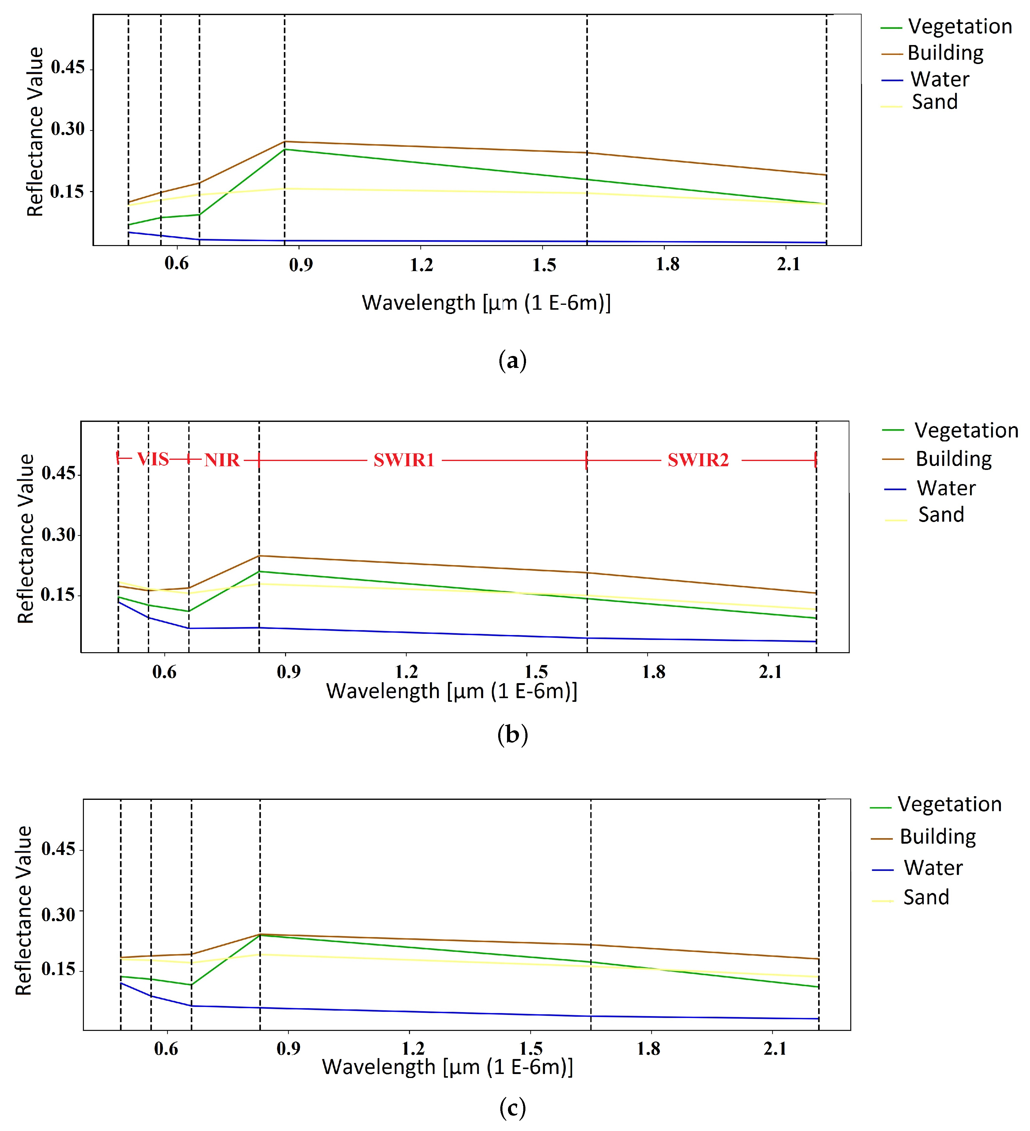
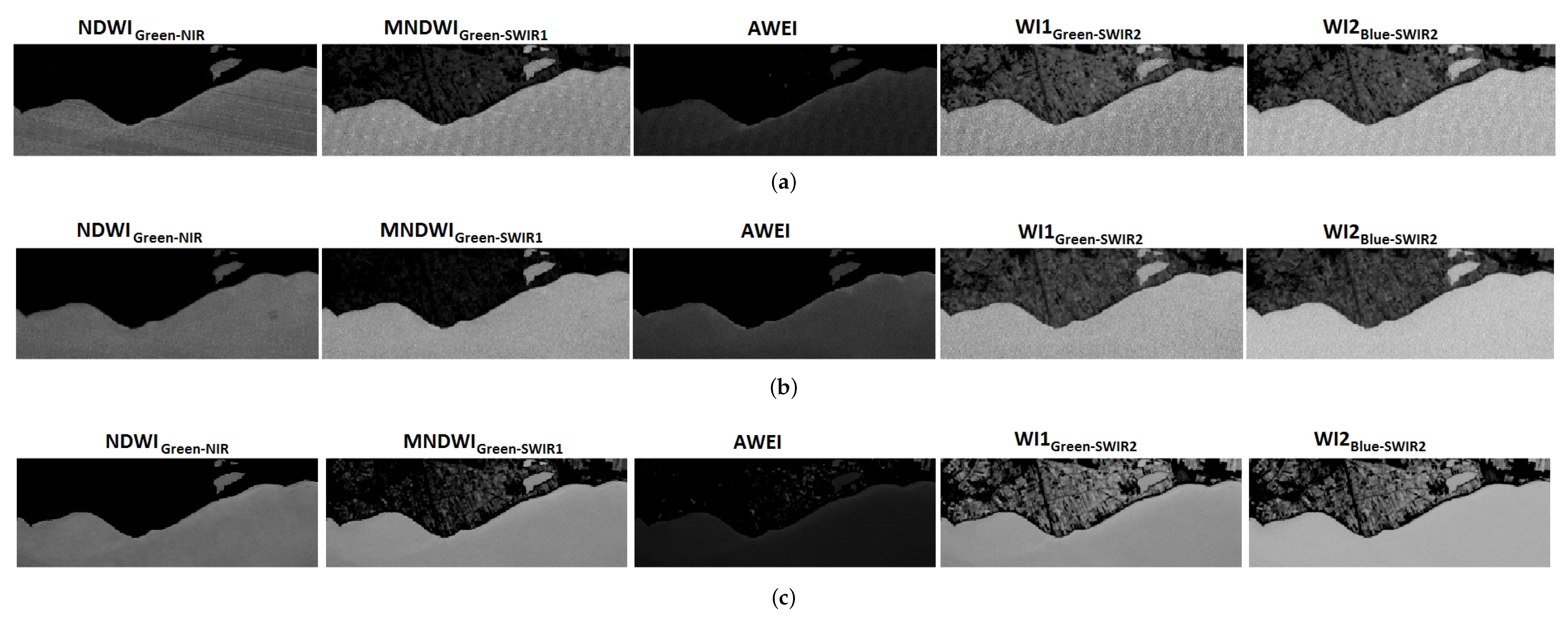
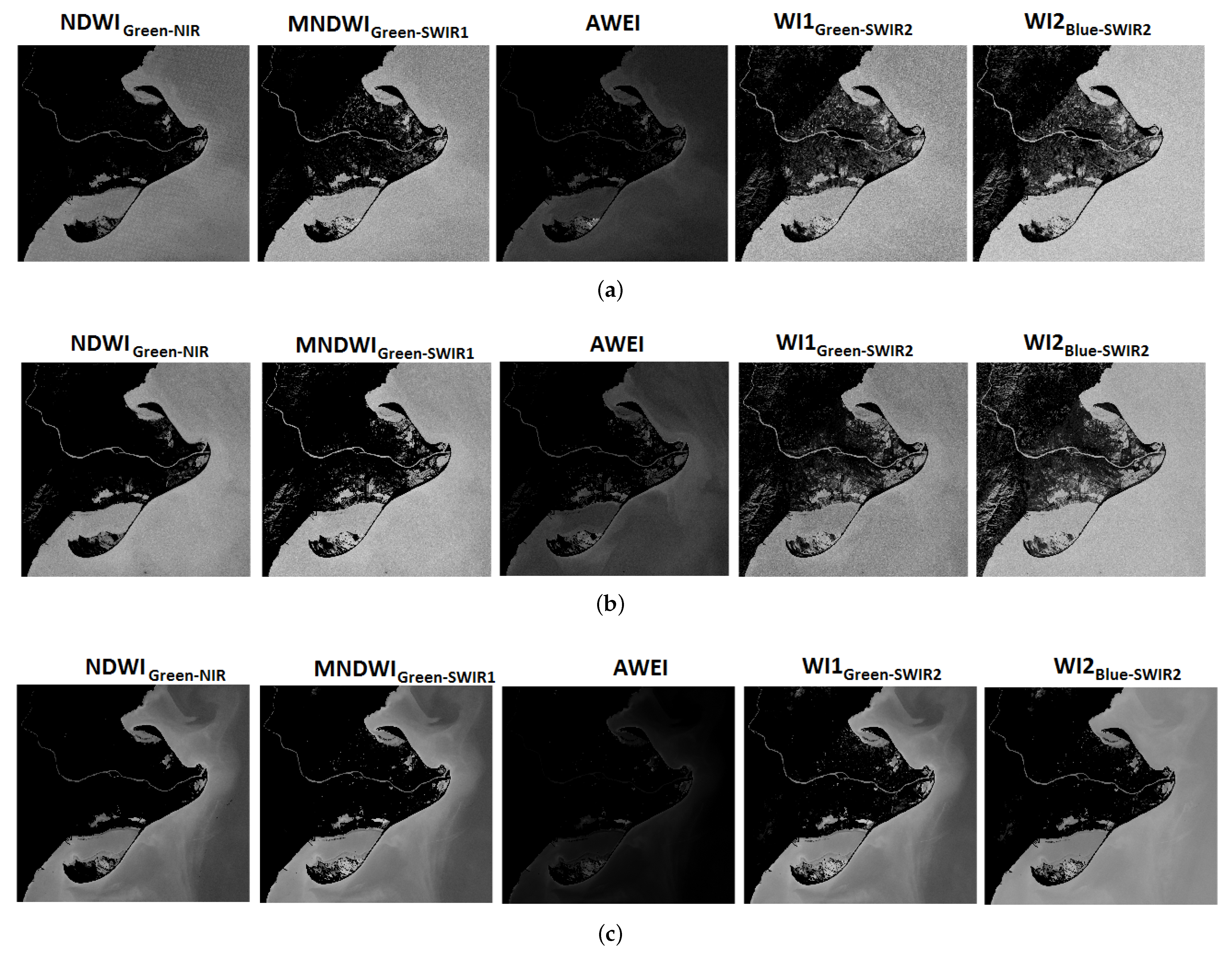
In this work, two new water indexes are proposed to identify the coastline based on the assumption that a spectral reflectance signature of water bodies is quite different from that of vegetation and soils. According to Chuvieco [93], water reflectance is higher in the VIS region and decreases when increasing the wavelengths, which means that water reflectance approaches zero in the NIR and SWIR regions in contrast to soil and vegetation of which reflectance increases significantly.

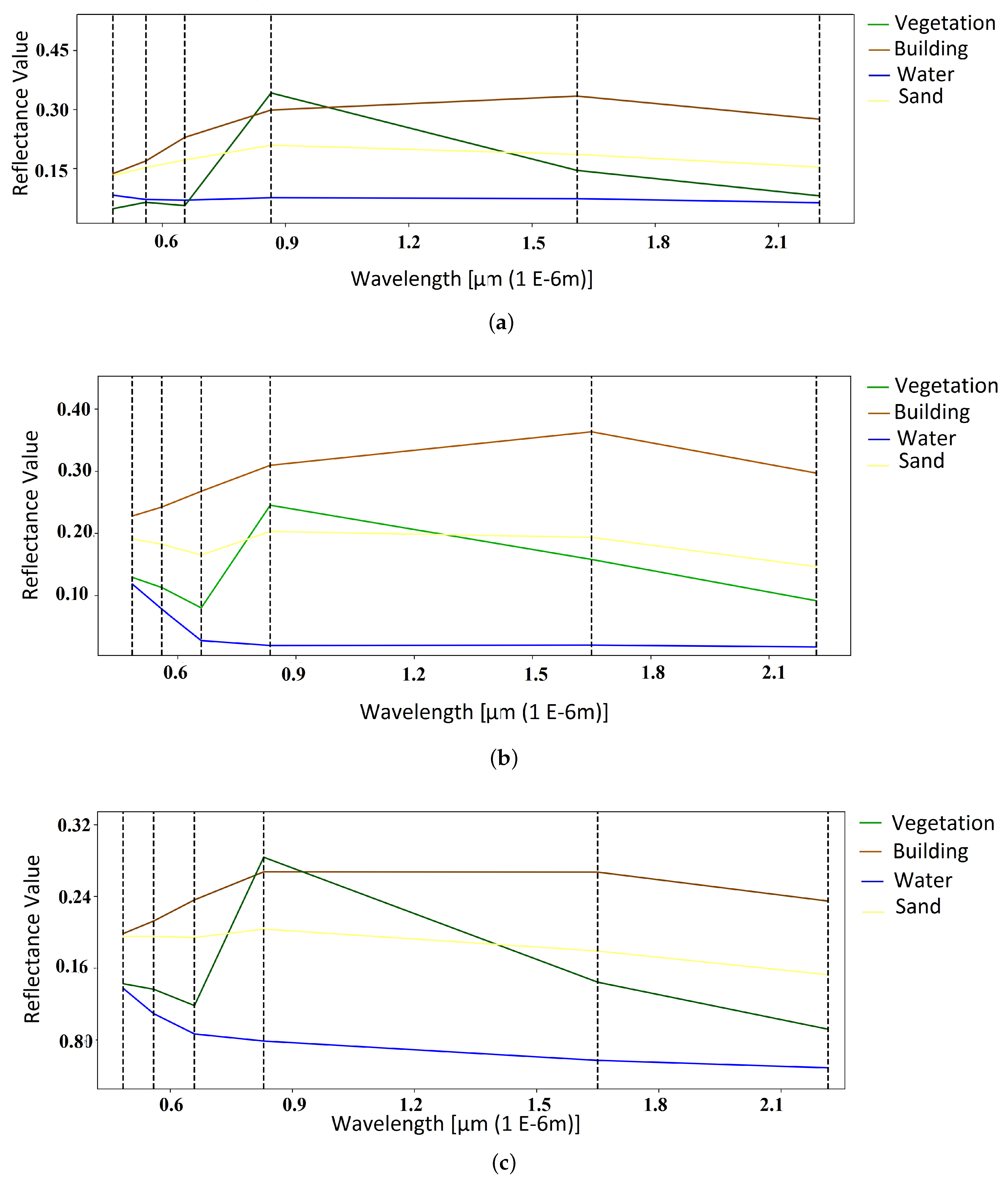
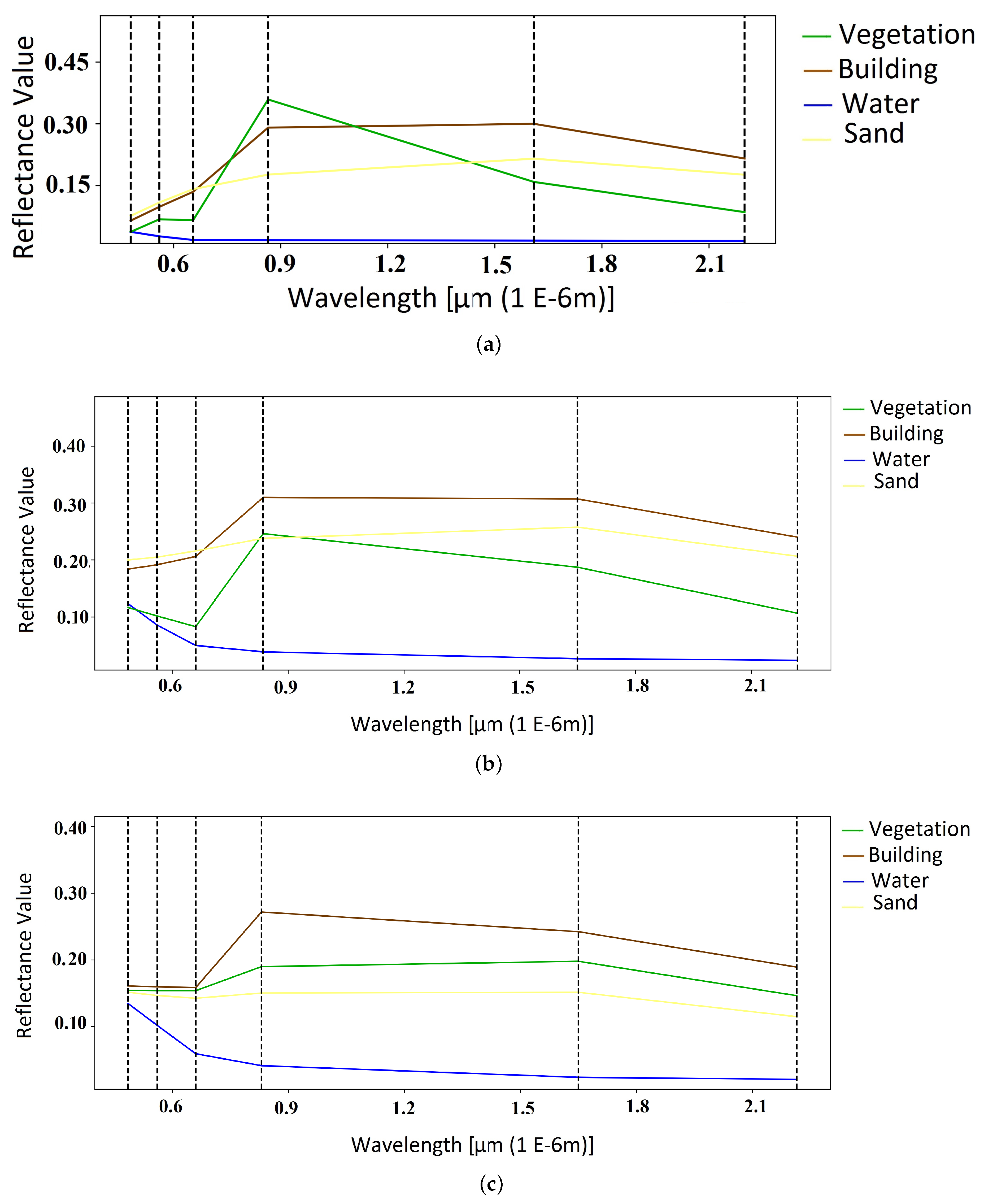
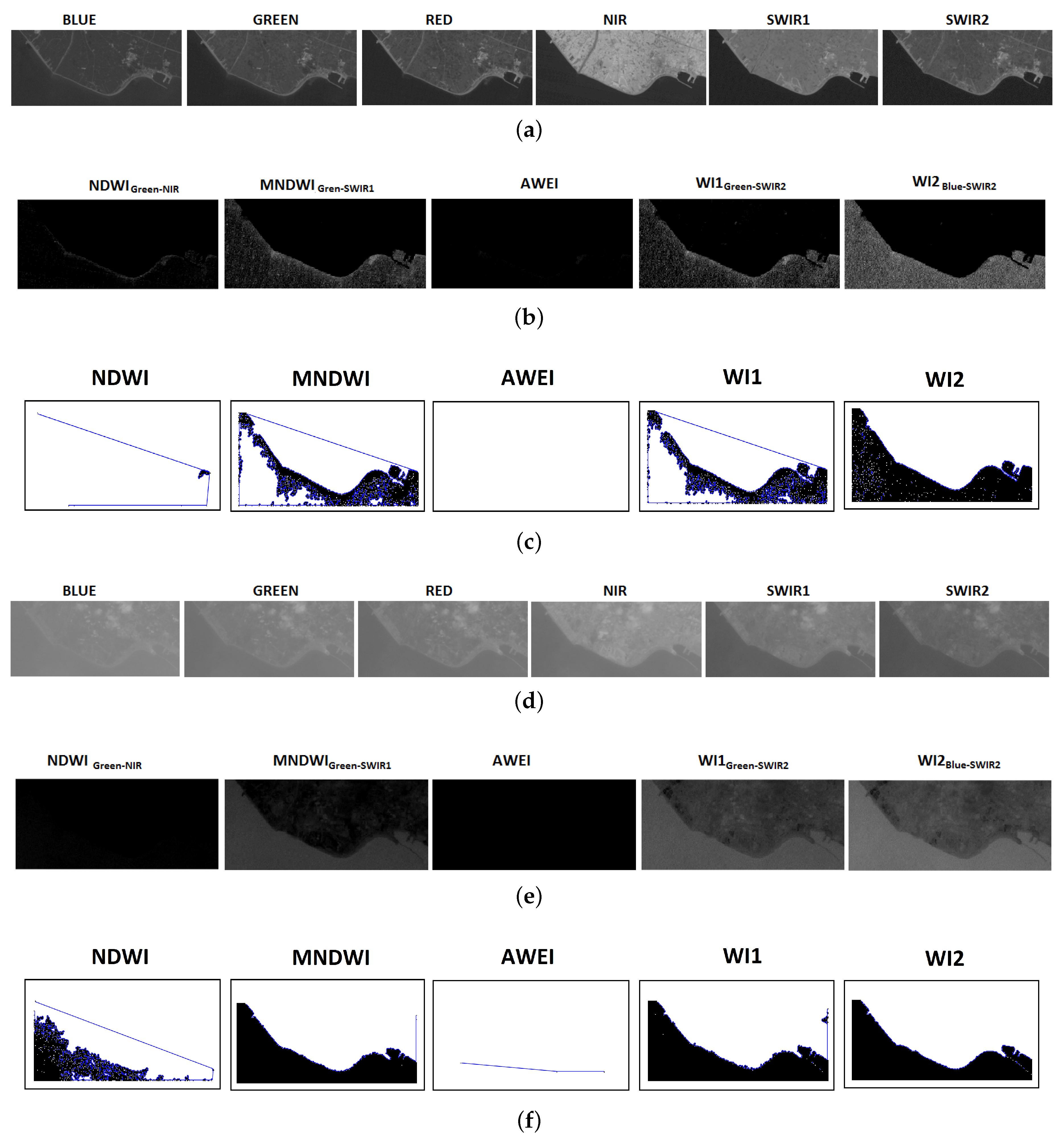
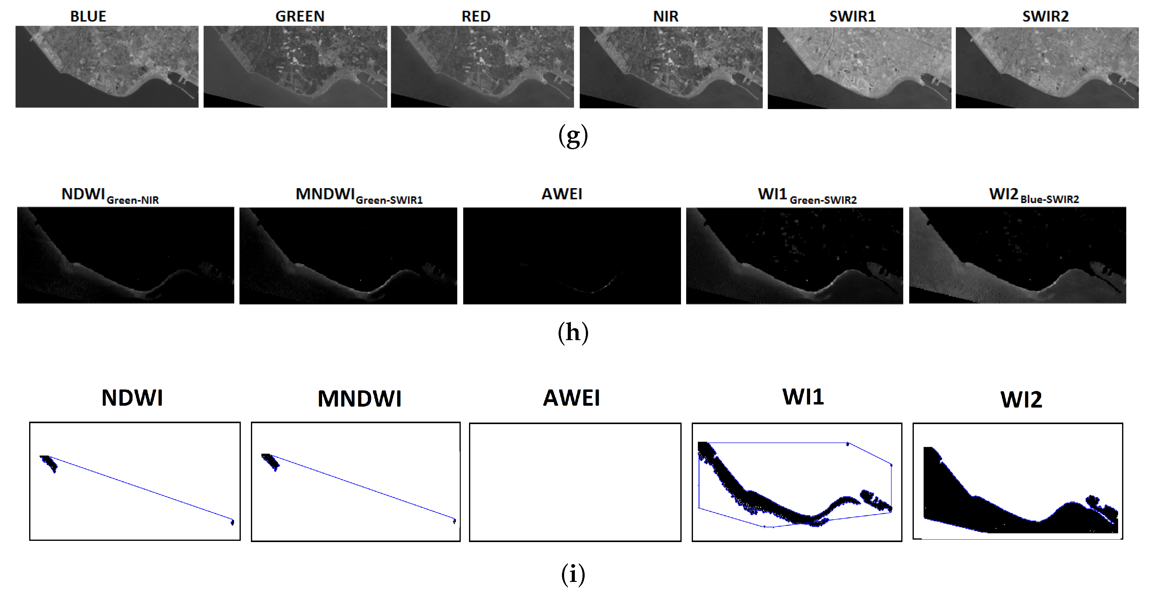
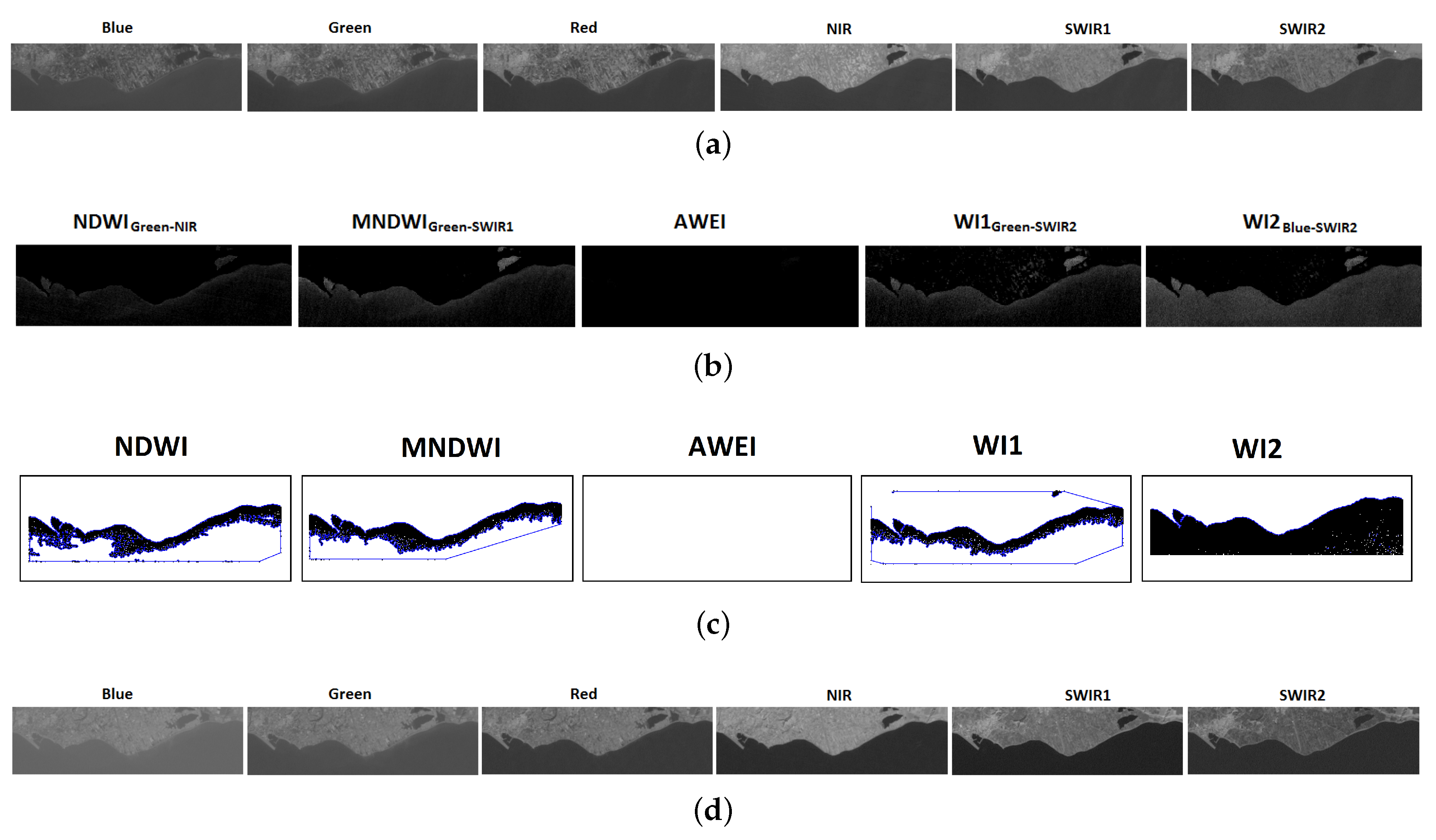
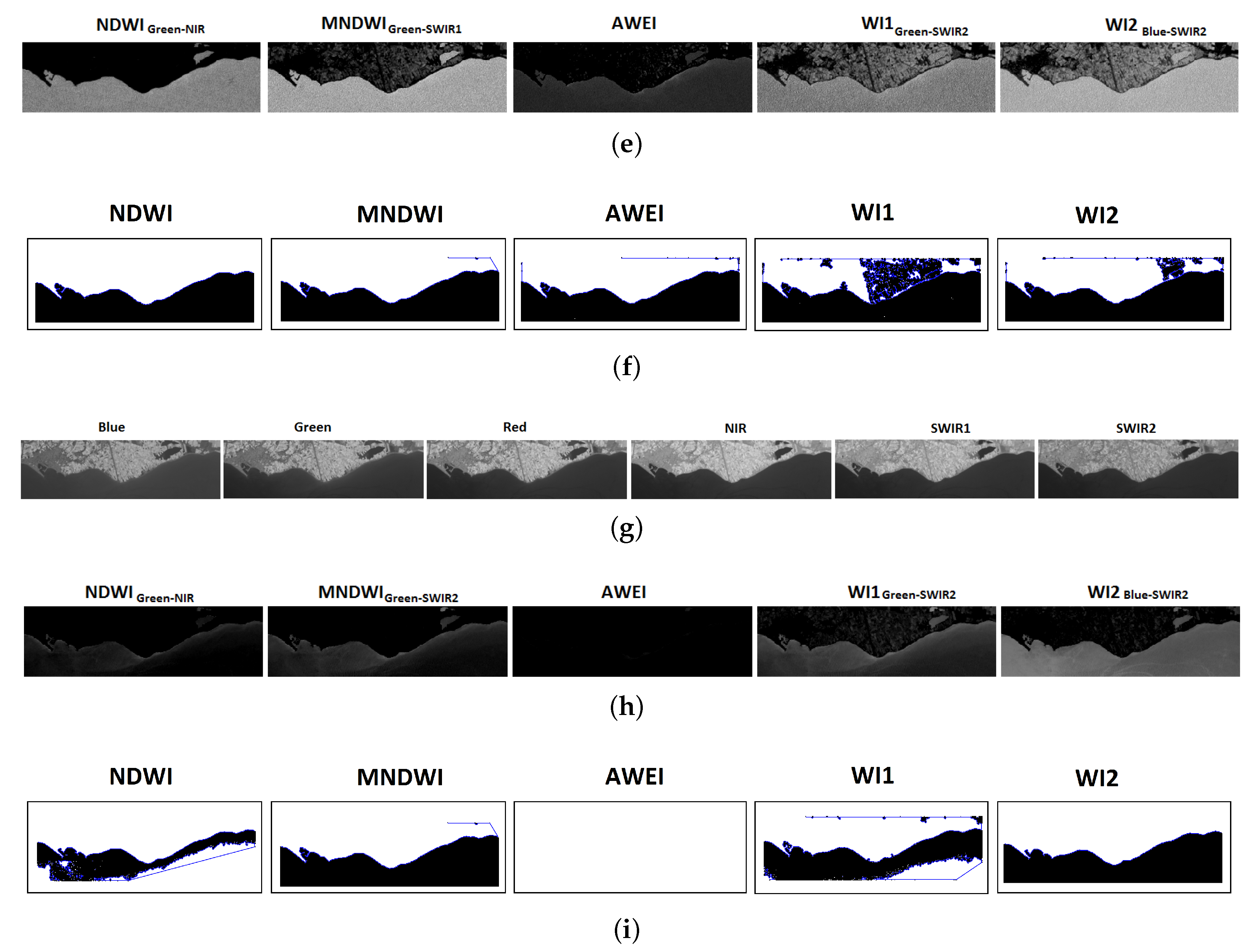
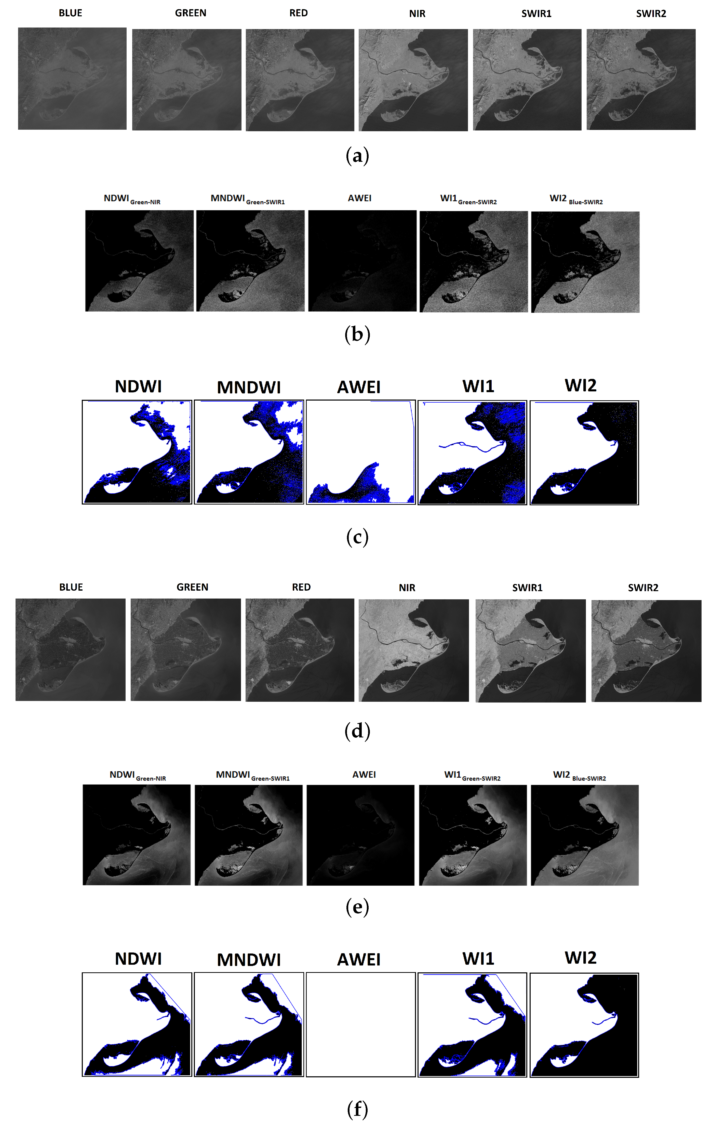
In this research, the spectral signatures of different land covers were analyzed from selected images of the Guadalfeo, Adra, and Ebro river deltas (Figure 3, Figure 4 and Figure 5). These spectral signatures allow to compare the land cover spectral behavior of the different sensors for each band. It was observed that the highest water reflectance was attained in the blue band, followed by the green one. However, the lowest water reflectance was found on the SWIR 2 band for all sensors. Thus, the proposed indexes were as follows:

$$WI1=\frac{{\rho }_{Green}-{\rho }_{SWIR2}}{{\rho }_{Green}+{\rho }_{SWIR2}}$$

(1)

$$WI2=\frac{{\rho }_{Blue}-{\rho }_{SWIR2}}{{\rho }_{Blue}+{\rho }_{SWIR2}}$$

(2)

where ${\rho }_{Blue}$, ${\rho }_{Green}$, and ${\rho }_{SWIR2}$ represent the surface reflectance in the green, blue, and shortwave infrared 2 bands, respectively.

The spectral signature of the different land covers from the three deltas tested is quite similar in terms of blue and SWIR2 band spectral behavior. From Figure 3, Figure 4 and Figure 5, it is noticeable that changes in the spectral behavior of the sand beach is almost imperceptible. Usually, NDWI and MNDWI are based on the assumption that spectral behavior of non-water covers have similar behavior in the green band but opposite in the NIR or SWIR1 bands. Although they usually give negative index values for non-water pixels and positive index values for water pixels, this is not always the case, as can be seen in different images analyzed as the TM image from Guadalfeo Delta river (Figure 3c), the TM and ETM+ image from Adra delta river (Figure 4b,c, as well as the TM image from Ebro delta river (Figure 5c), in which, if MNDWI was calculated, sand pixels would take positive values just as water. This can result in sand pixels misinterpreted as water pixels, so the accuracy of the coastline detection decreases. The presence of sand is an important issue because sand reflectance may vary depending on sand color or grain size of sediments and the content of water, as Drakopoulos et al. [94] confirmed by laboratories measurements.

On the other hand, as can been seen in all the spectral signatures from the three deltas tested, if WI1 and WI2 are calculated in any of the images of Figure 3, Figure 4 and Figure 5, they will usually get positive pixels values but non-water pixels will get values close to zero or negative while water pixel values will be much higher. Thus, these differences in pixel values would help the Otsu’s algorithm performs better in segmentation processes since this method maximizes the between-class variance and minimizes the within-class variance [95].

5.1. Preprocessing Phase

The preprocessing process was done using open source Quantum GIS (QGIS) software. The Semi Classification Plugin (SCP) allows not only for the semi automatic classification of remote-sensing images but also for the preprocessing of images and raster calculations [96]. Using SCP, digital numbers of each Landsat image selected were converted into radiance and then into surface reflectance by applying the Dark Object Subtraction (DOS) method [97]. Prior studies have compared the DOS method to other atmospheric correction models over water areas and urban coastal environments, showing that DOS exhibits better performance, being one of the atmospheric correction models widely used in coastal studies [7,29,31,98]. Surface reflectance was used rather than TOA reflectance since atmospheric correction is needed for analyzing multiple images acquired from different satellite sensors [99,100]. Parameters required for preprocessing were extracted from metadata files downloaded with image data products. To find out more about how the radiometric normalization and the atmospheric correction was calculated, see Appendix B.

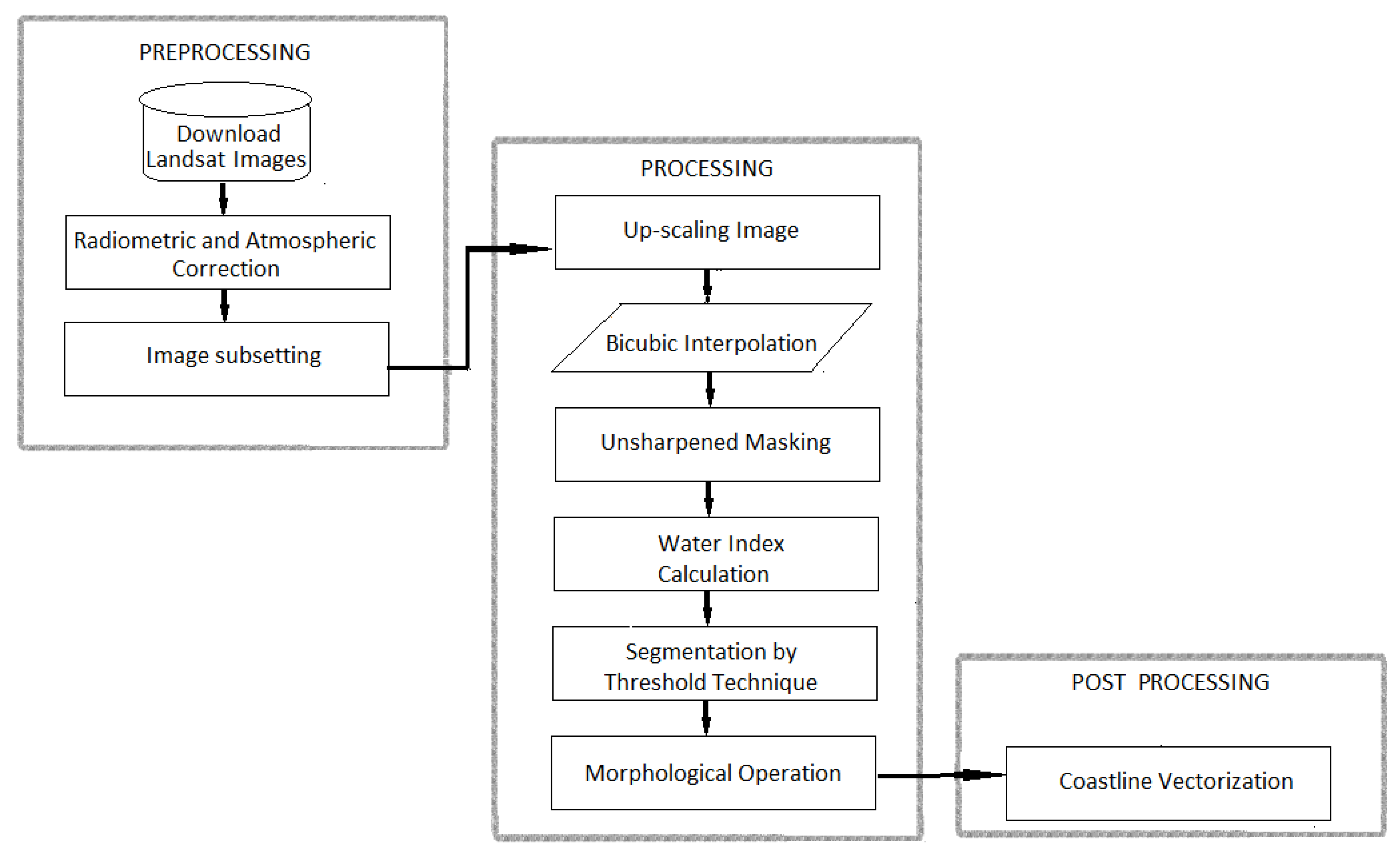
5.2. Processing Phase

The processing step was made using Matlab®. First, each band image was subset to extract the study area in the first part of the automatic algorithm developed; this part allows to select all the original size Landsat images needed from the same zone. When all the images are loaded, the algorithm asks for the desired area to be cropped in the first image. The algorithm user points out the desired area, and the algorithm saves the coordinates selected in the image and applies the crop to the rest of the images with the same parameters. The next step was to apply a Matlab built-in function of unsharp masking (i.e., an image sharpening subtracting a blurred version of the image from itself [101]) to enhance the edges presented in the images [102]. 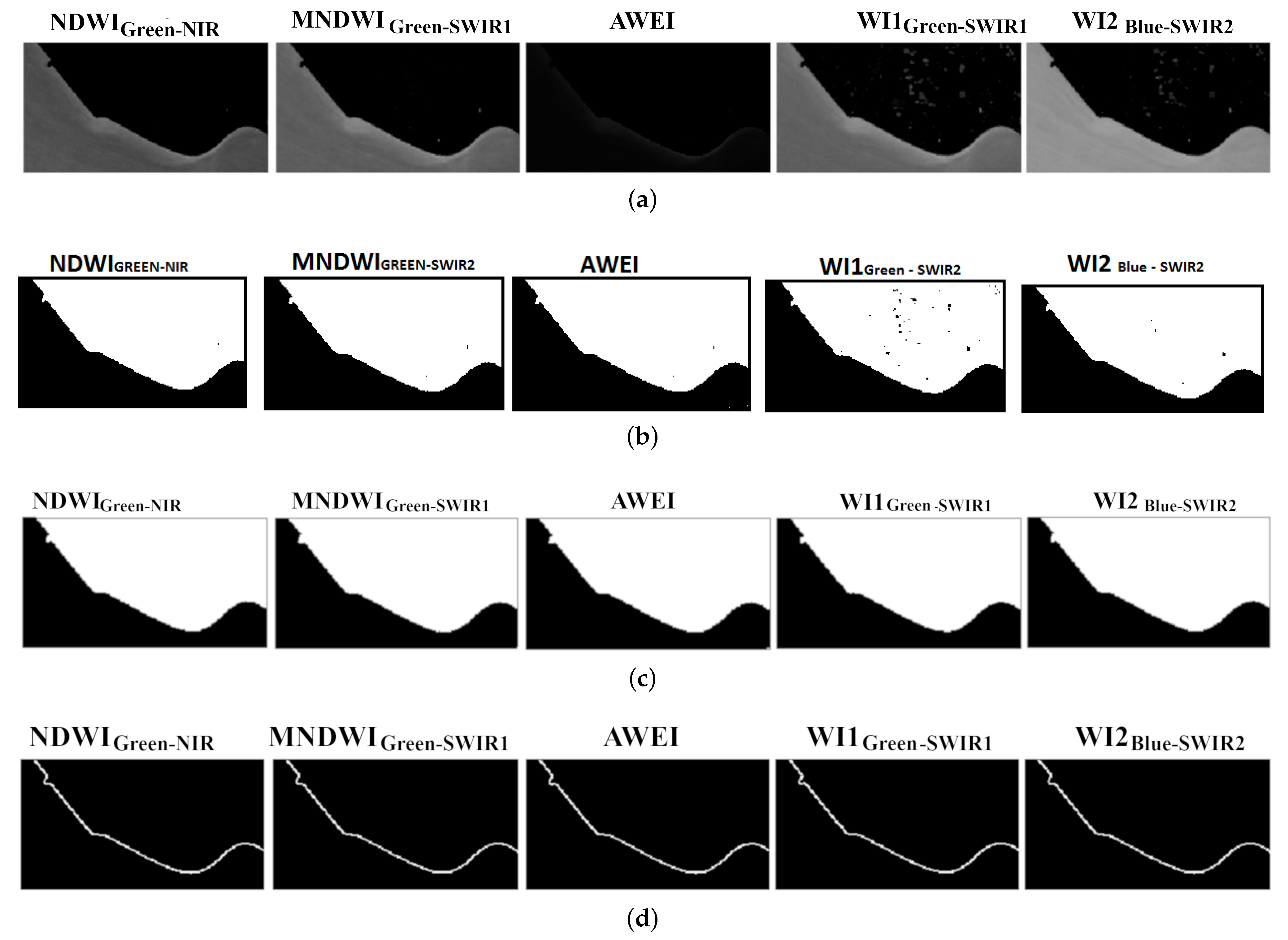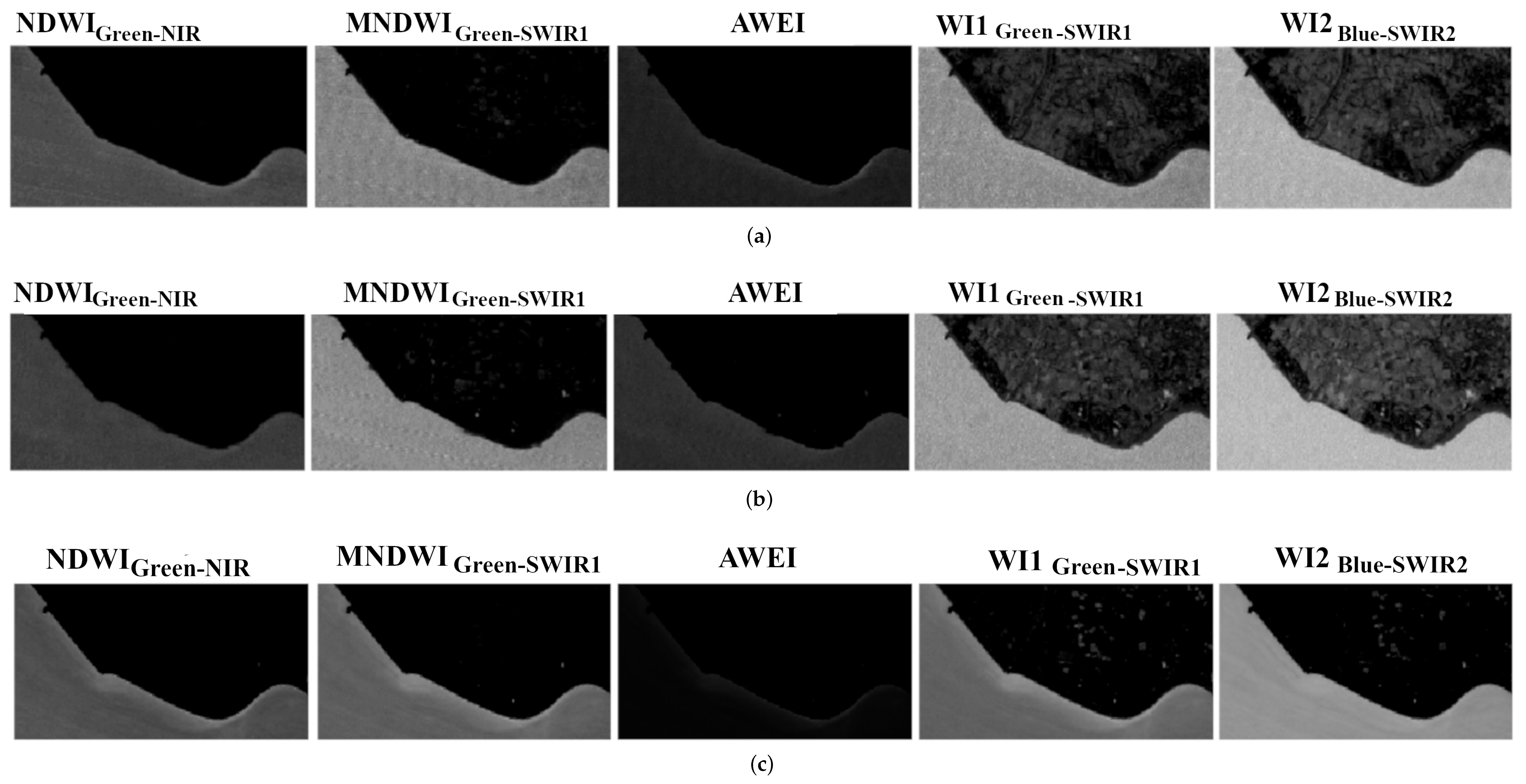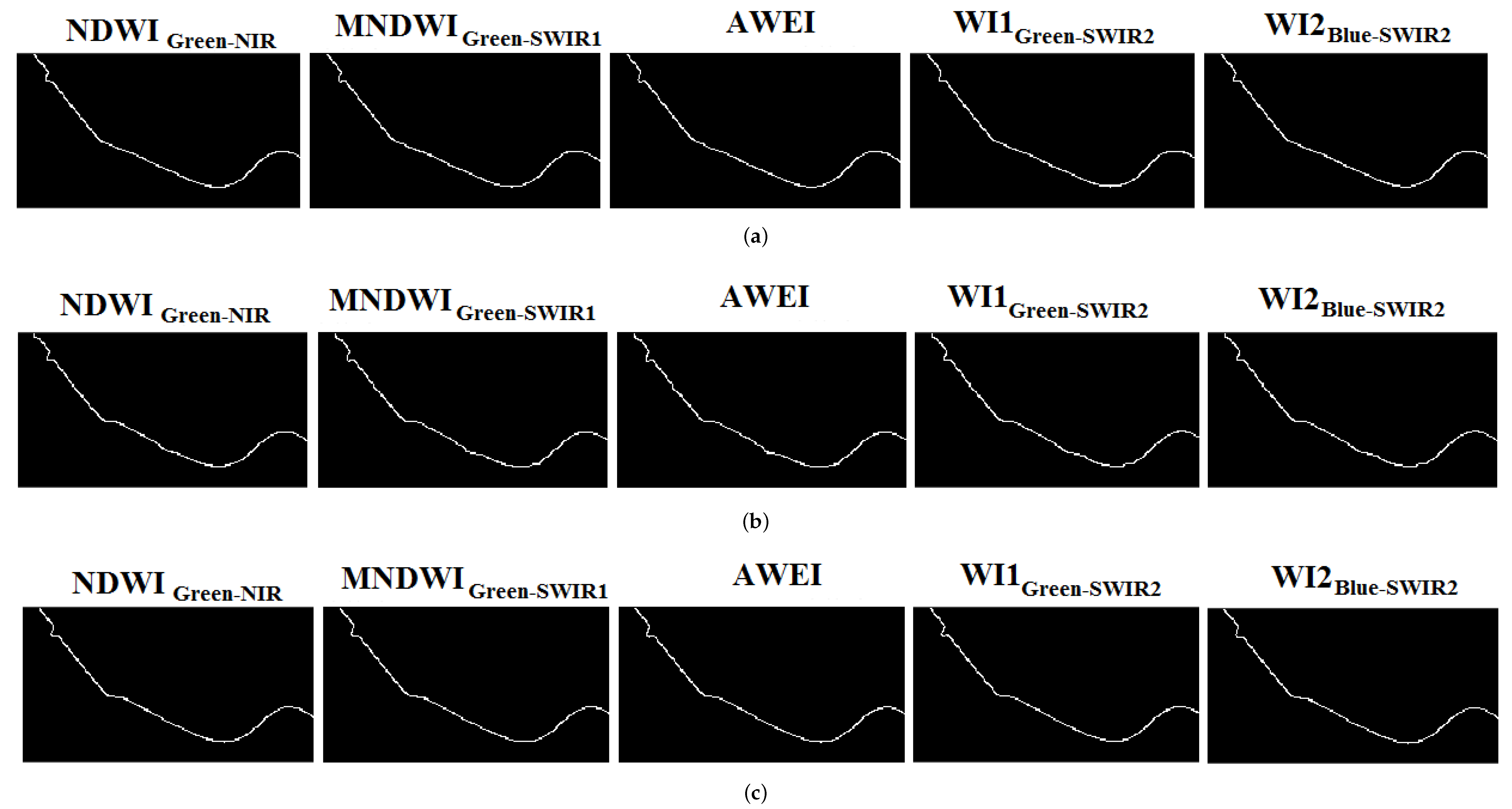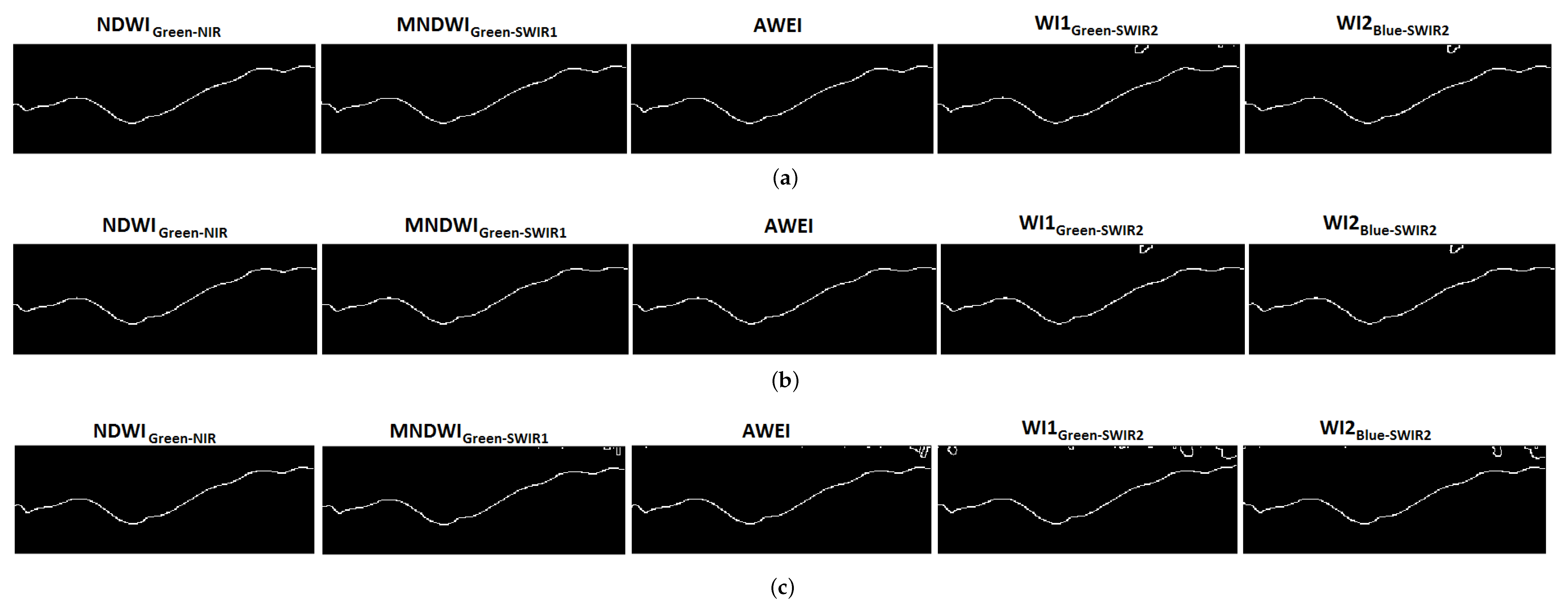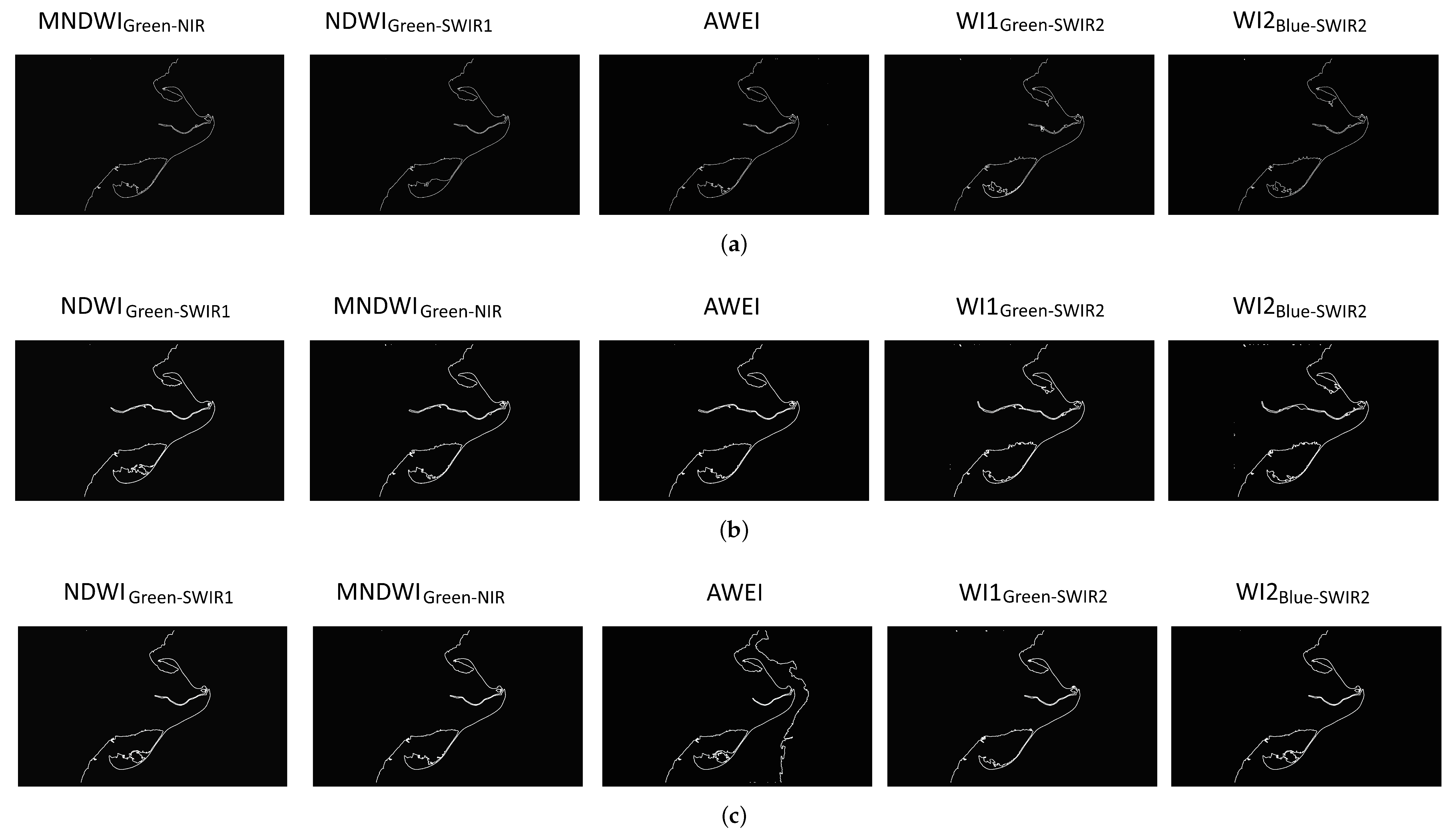Then, the water indexes were applied according to Equations (1) and (2) for the proposed water index (WI1 and WI2, respectively), and the expressions found in Table A3 for the water indexes were selected to compare the proposed ones (NDWI, MNDWI, and AWEI). After the application of the water indexes, the segmentation step was performed to produce a binary image by threshold technique. In segmentation techniques, an image is partitioned into meaningful parts, which have similar features and properties [103]. This method permits to extract objects by selecting a specific threshold to differentiate the object from the background. Otsu’s method [104] was selected as the global threshold automatic selection method because it is widely used [105] and it is one of the best threshold methods of general real-world images with regard to uniformity and shape measures [95]. Otsu’s method assumes that the image has two kind of pixels that either fall in a foreground class or background class, so iterations are made until an optimal threshold value that separates both classes is found.

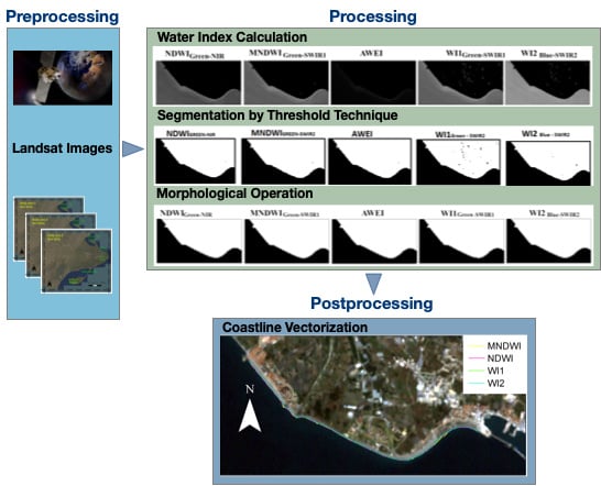
Once a binarized image is obtained, a morphological operation is applied to clean up the image, removing useless pixels. The morphological operation was an imfill built-in Matlab function to fill all the holes inside the land area. Finally, a vectorization step was performed to obtain the coordinates of the coastline extracted. An example of the sequence of the methodology applied on every image can be seen in Figure 6 from an image obtained in the Guadalfeo delta on September 12, 2013 by the OLI sensor.

This methodology was applied to original-size Landsat images and to increased spatial resolution images for further assessment of accuracy improvement. We used bicubic interpolation because it offers the best results compared to different linear up-sampling methods [37,39,106,107] in spite of its simplicity [108,109].

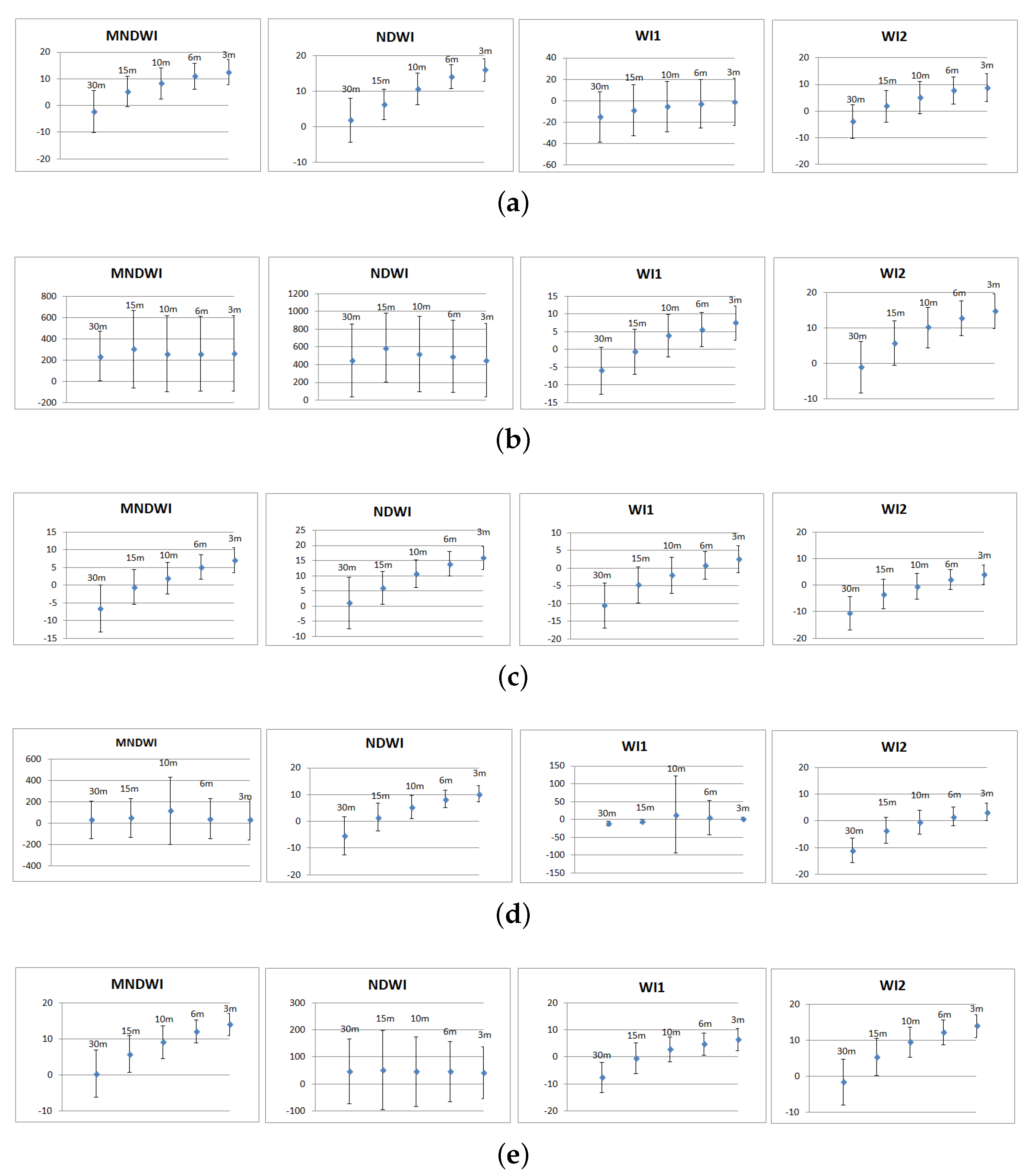
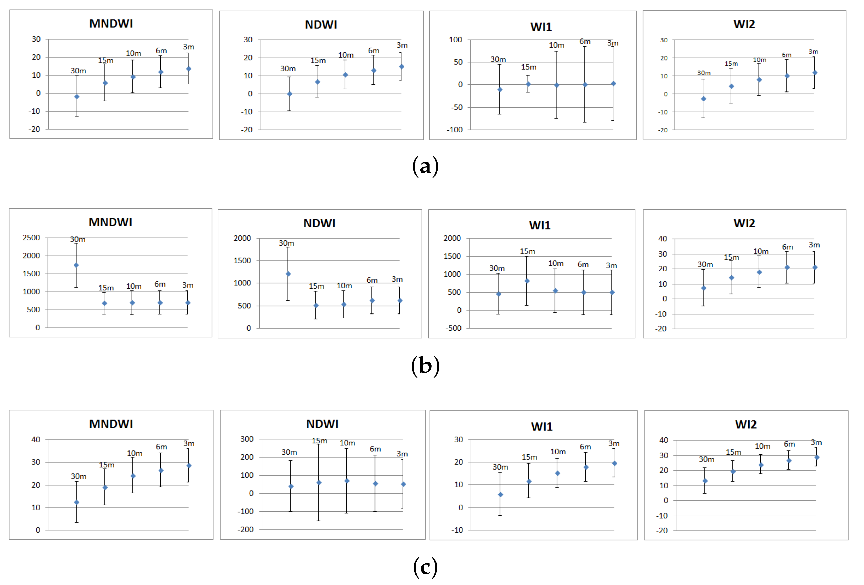
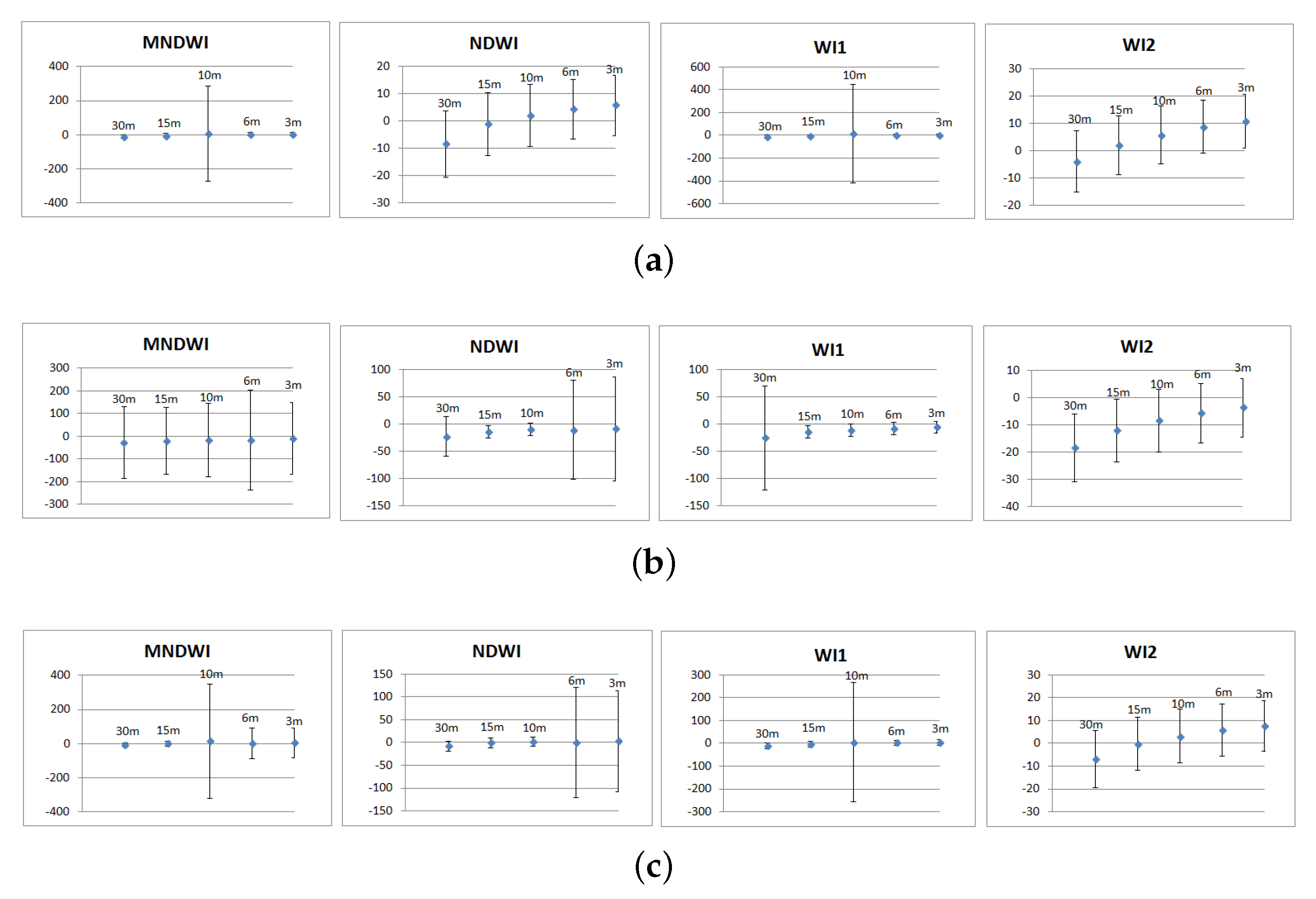
The spatial resolution increase was assessed by detecting the coastline with the original spatial resolution image (30 m/pixel) and then by testing bicubic interpolation with different factors of up-sampling to assess if the accuracy of the detected coastline with WI1 and WI2 could improve. We assessed bicubic interpolation with factors of 2 (15 m/pixel), 3 (10 m/pixel), 5 (6 m/pixel), and 10 (3 m/pixel).

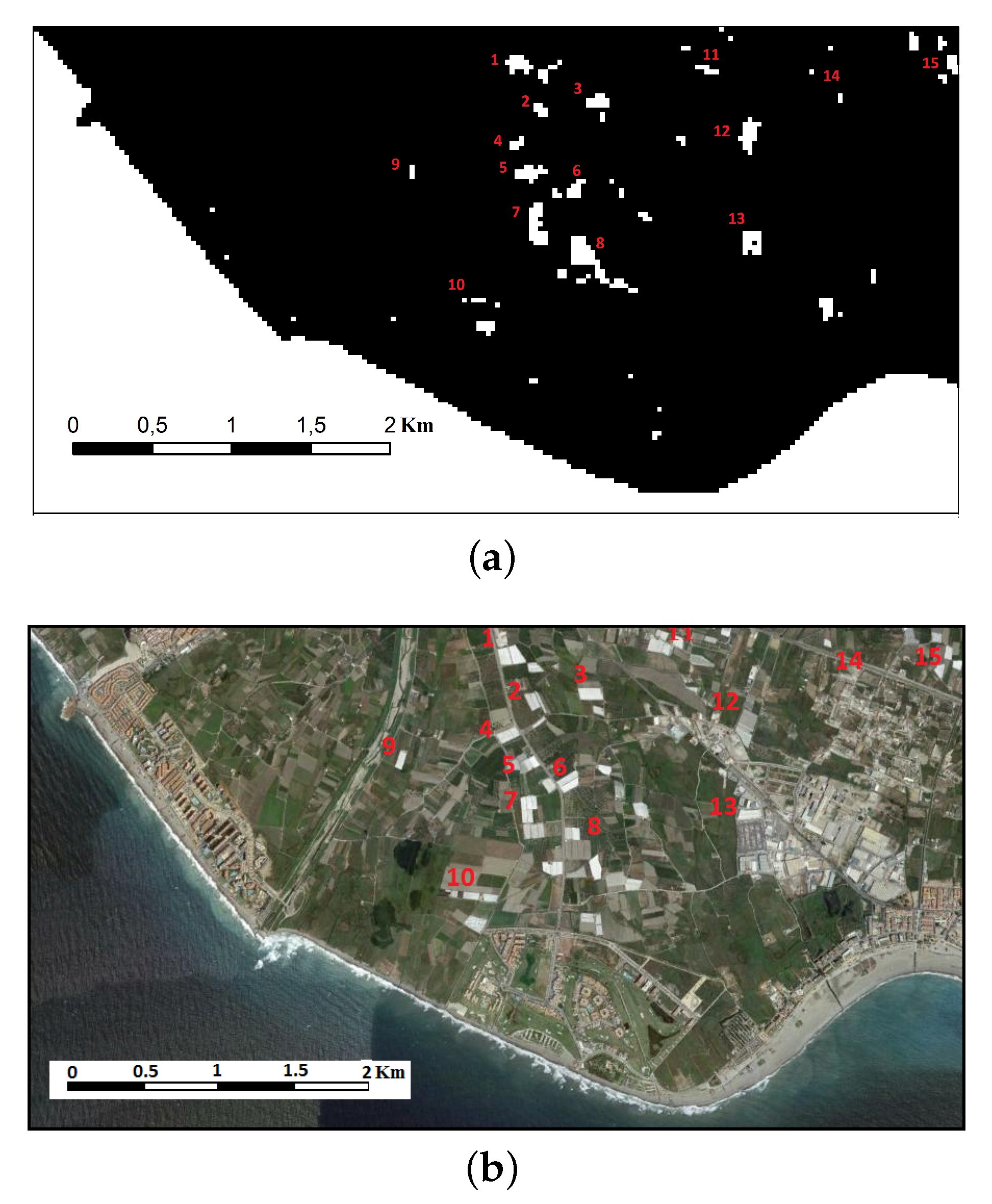
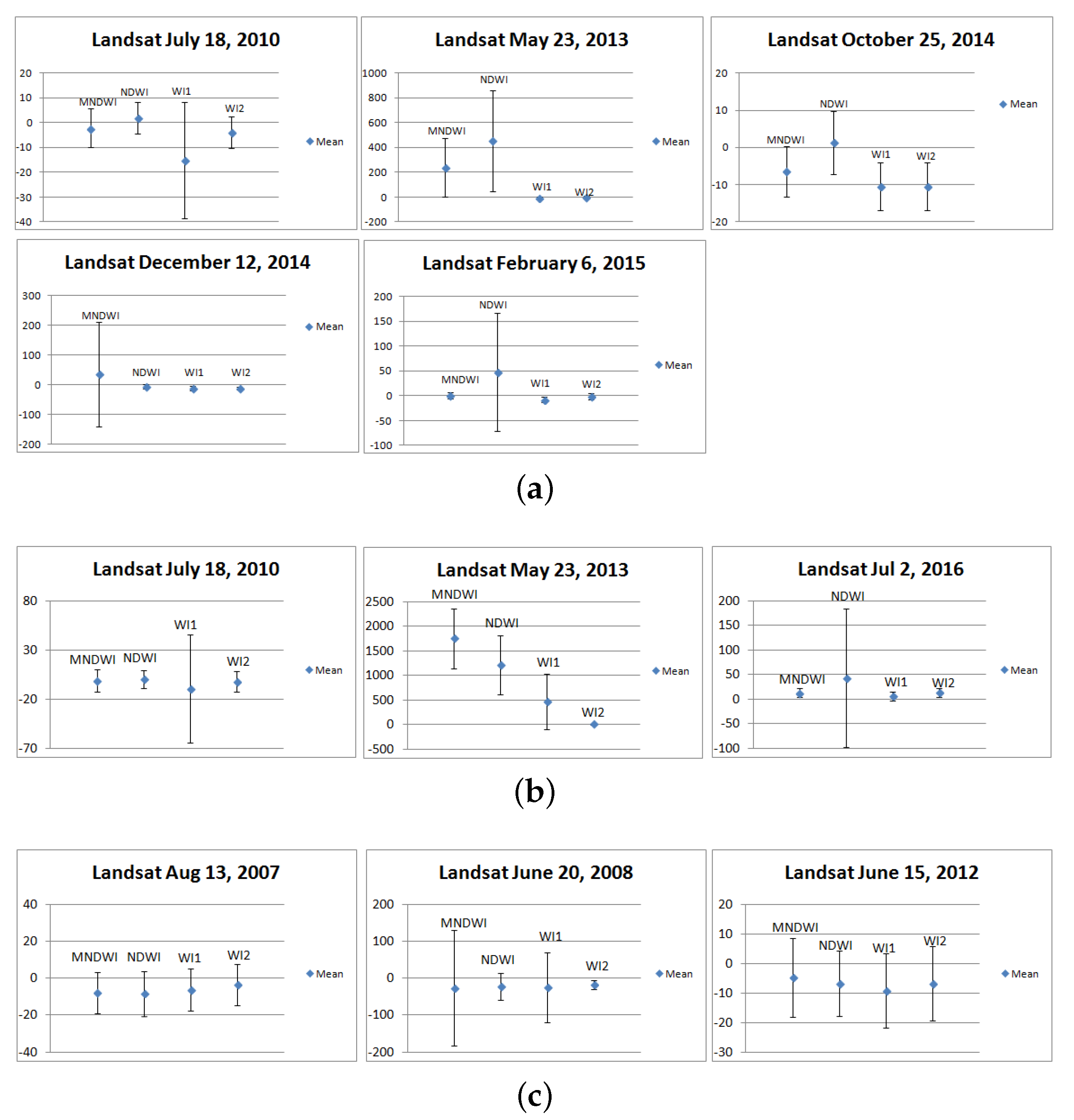
5.3. Data Validation

The methodology proposed was applied using NDWI, MNDWI, and AWEI indexes and then compared to the coastline extracted with the new water indexes proposed WI1 and WI2. The statistic metric used to analyze the goodness of the different indexes were the mean and the standard deviation of the distances between the shoreline extracted from high-resolution data and from the Landsat images. It was calculated as follows:

$$Mean=\frac{{\sum }_{j=1}^n\left(Y{j}_{Hr}-Y{j}_{LS}\right)}{n}$$

(3)

$$Dj=\left(Y{j}_{Hr}-Y{j}_{LS}\right)$$

(4)

$$\mathit{STD}=\sqrt{\frac{{\sum }_{j=1}^n{\left(Dj-Mean\right)}^2}{n}}$$

(5)

where

• Dj = Distance in meters between the high resolution data and the data derived from the Landsat images. The difference of the vertical distance between the shorelines compared for the same X coordinate was calculated. Dj is a positive value as Landsat data is seaward, and if Dj is a negative value, it means that the Landsat data is landward.
• Yj_LS = Coordinate of the Landsat data.
• Yj_Hr = Coordinate of the high-resolution data.
• Mean = The mean of Dj in meters.
• STD = Standard deviation of Dj in meters.
• n = Number of elements of the data evaluated.

6. Results

6.1. Coastline Extraction at the Pixel Level

We applied the methodology proposed for coastline extraction to Landsat images in the Guadalfeo, Adra, and Ebro deltas. Each pixel value or digital number (DN) of these images was transformed to spectral radiance and then converted into surface reflectance values, as explained in Section 5.1. An example of the sequence of the methodology applied to every image can be seen in Figure 6 from an image obtained in the Guadalfeo delta on September 12, 2013 by the OLI sensor.

It can be observed through a visual comparison that the methodology applied using the water indexes WI1 and WI2 were able to separate water from non-water pixels across the study areas covered. WI1 and WI2 were more sensitive in detecting vegetation areas than the other indexes, as can be seen in Figure 7, Figure 8 and Figure 9 in the TM and ETM+ images.

The Ebro delta is a more complex area in a geomorphological characterization sense due to the presence of coastal lagoons, salt marshes, and narrow long sand bars. In contrast to TM and ETM+ images, in the OLI images after WI1 and WI2 was applied, the vegetation area was not detected but the salt marshes, the different lagoons inside the area, and the course of the river were still present, which is consistent with the goal of detaching water pixels from non-water pixels.

The non-water pixels (vegetation/greenhouses areas) that presented in TM/ETM+ images after applying WI1 and WI2 were eliminated with the segmentation and morphological operation steps, as seen in Figure 6b,c. Apparently, after applying the methodology, the visual comparisons for both Guadalfeo and Adra deltas (Figure 10 and Figure 11) show a similar coastline detection with all the water indexes applied, including the proposed WI1 and WI2. In the Ebro delta case (Figure 12), there are some variations, especially in the inner side of the coastline of the Banya spit.

Some of the non-water areas detected were associated with greenhouses, as seen in Figure 13, regarding the Guadalfeo delta area, where the noise identified in the analyzed image matched some greenhouses found in a high-resolution image. This greenhouse-related behavior is more evident in the Adra delta, where most of the land is dedicated to this use, so the three sensors detected the greenhouses areas (see Figure 8). However, the contrast between the sea water and the shoreline is slightly better when obtained with WI1 and WI2. Furthermore, after application of the methodology, WI1 and WI2 detect the shoreline, avoiding non-water areas.

In the visual comparison across the entire set of images, we found that, in the Guadalfeo delta, AWEI was not able to detect the coastline in 43.19% of the images. The OLI sensor presented a higher number of images by which AWEI could not detect the coastline (54.69% of the OLI images). Moreover, in 19.70% of the total images analyzed, AWEI detected noise around the coastline, which makes the result useless. NDWI and MNDWI showed noise around the coastline in almost 12.88% and 11.36% of the images, respectively. This behavior was observed in 25% of TM images and in 18% of OLI images. In addition, NDWI and MNDWI were not able to detect the coastline in almost 4.90% and 11.36%, so in these cases, these indexes were not useful. Instead, WI1 was able to detect the coastline in 85.98% of the set of images but showed noise in almost 7.33% of them, while WI2 was the only index that was able to detect the coastline in almost all the scenes that were analyzed (99.62%). Figure 14 shows examples of no coastline being detected or the noise that presented in some of the images after applying the methodology with the different water indexes that were evaluated.

Regarding the Adra delta, the results after applying the methodology to the images point to a similar behavior as that of the Guadalfeo delta. According to

Table 3. Number of images that has no error or noise after applying the methodology for coastline detection with the different indexes evaluated.

STUDY ZONE	SENSOR	No OF IMAGES	NDWI	MNDWI	AWEI	WI1	WI2
Guadalfeo	TM	264	30	31	24	25	50
	ETM+		146	145	113	149	149
	OLI		41	28	24	50	64
Adra	TM	172	39	39	25	26	56
	ETM+		50	50	40	32	46
	OLI		34	36	9	49	58
Ebro	TM	185	24	24	17	24	35
	ETM+		104	104	43	104	104
	OLI		7	8	0	8	102

, in the TM and OLI images, the AWEI index showed more scenes (72.53% of the TM images and 85.25% of the OLI images) that were not able to detect the coastline or presented too much noise, which need further image processing or a different methodology, for example. In addition, WI1, MNDWI, and NDWI presented a significant proportion of results with no coastline or too much noise (approximately 37.80%, 27.33%, and 36%, respectively). However, WI2 showed better performances in detecting the coastline, with only 6.92% of the images, whereby the methodology could not obtain useful results. The results from the ETM+ images showed that MNDWI, NDWI, and WI2 behaved in a similar manner, giving the best outputs and obtaining a useful coastline from almost all the images. For a while, AWEI and WI1 gave a satisfactory result in more than 64% of the ETM+ images. In Figure 15, the common error that presented in the analyzed images from Adra delta can be seen.

For the images analyzed from Ebro delta, WI2 showed by far the best result in detecting the shoreline for both OLI and TM images, with 88.9% and 100% of the images, respectively, in comparison with those of MNDWI (22.2% of the OLI images and 53.3% of the TM images), NDWI (19.4% of the OLI images and 53.3% of the TM images), and AWEI (0% of the OLI images and 37.77% of the TM images). Nevertheless, for the ETM+ sensor, the indexes compared (except AWEI) could detect the coastline in the entire set of images from that sensor. Figure 16 shows some of the errors after applying the methodology to detect the coastline.

In general, as seen in Table 3, the best performance according to accurate coastline detection was WI2, which detected the shoreline in 95.65% of the total of images that were analyzed, including the three deltas. WI1, MNDWI, and NDWI obtained similar results (75.65%, 74.9%, and 74.50%, respectively). The worst result was obtained by AWEI, which detected the shoreline in only 45.75% of the total of images that were analyzed in this paper.

6.1.1. Accuracy Assessment

The Landsat images that were selected from the three study zones were compared to field measurements that were collected with a differential global positioning system (DGPS) and/or with high-resolution orthophotos. The statistical validation was performed for pixel and sub-pixel analyses of each of the evaluated images by calculating the bias (mean ± standard deviation), as described in Section 5.3. Each high-resolution data gives a coastline to be compared with the coastline that was detected in the Landsat images after applying the methodology using the water indexes that have commonly been used in the literature as well as the water indexes proposed in this research. The statistical results are plotted for visual comparison in Figure 17, Figure 18, Figure 19 and Figure 20, where the AWEI index was excluded due to its unsatisfactory results in detecting the coastline along the analysis. Appendix D shows the numerical results that were obtained for bias and standard deviation calculations, including AWEIs.

Pixel Level

First, we compared at the pixel level the difference in distance between the coastline detected with the high resolution data and those detected with the different water indexes used in this paper. Based on the Landsat image recorded on May 23, 2013, WI1 and WI2 were the only two indexes that were able to detect the coastline; the rest of the evaluated indexes showed too much noise due to misidentification of water pixels as land pixels, and the bias and precision that were obtained with WI1 and WI2 were also satisfactory.

According to the statistical results, the pixel analysis in the Guadalfeo delta (Figure 20a) showed that, for most of the dates evaluated in this study area (three of five), the shorelines detected with NDWI had the lowest seaward bias; however, the standard deviations in both NDWI (ranging between ±6.22 and ±119.40) and MNDWI (±6.48 and ±175.25)) were much higher and heterogeneous than those obtained in shorelines detected with WI2 (±4.70 and ±7.29), which means that shorelines detected with the WI2 method are more precise and stable than those detected with the rest of the indexes. In addition, WI2 reached the minimum value of bias (−0.91 m).

Figure 20b shows the bias and standard deviation calculated between shorelines detected from high-resolution data and the shorelines detected from Landsat images in the Adra delta. AWEI was again not taken into account because it has no useful result for any of the dates that were evaluated. The shoreline detected with WI1 on July 18, 2010 had a high standard deviation value due to a misidentification of land pixels as water pixels in the mouth of the Adra river area. The shorelines detected with the MNDWI, NDWI, and WI1 methods only showed one date with an acceptable standard deviation less than ±12.00. Therefore, in this study zone, WI2 had the best performance since it was the only index that had a bias less than 13 m for the three dates analyzed, with a homogeneous standard deviation less than ±12.50.

Figure 20c shows the graphs regarding the bias and standard deviation calculated between shorelines that were detected from the Landsat images and high-resolution orthophotos from the Ebro delta. The results obtained for these study zones were consistent with the results of the other two study zones. AWEI was also not plotted because it has no useful results for any of the dates that were evaluated. Once again, the shoreline detected with the WI2 method had the best performance since almost all the dates that were evaluated showed a lower bias and obtained a lower standard deviation, which means that the shorelines obtained with the WI2 method is a good approach for the expected shoreline.

Sub-Pixel Level

Although the Landsat collection is the largest collection of satellite images with moderate resolution, this resolution sometimes is not enough, depending on the type of analysis that is required. We applied a simple sub-pixel analysis to assess the position accuracy of the detected shorelines. However, the statistical results showed an increasing trend of bias, although the standard deviation remained nearly constant.

7. Discussion

7.1. Coastline Extraction at Pixel Level

The applied methodologies (with water indexes WI1 and WI2) were able to separate water from non-water pixels across the study areas covered, although WI1 and WI2 were more sensitive to detecting vegetation areas than the other indexes. This may be because both water indexes use the SWIR 2 band, which is useful for detecting the moisture content of soil and vegetation. However, WI1 and WI2 combined with Otsu’s segmentation were able to remove the building and beach sand areas next to the coastal zone, which is critical for dividing water from non-water pixels. The differences that were observed in the WI1/WI2 results between TM/ETM+ and OLI images may be due to technical differences between the sensors. The OLI sensor has better spectral resolution, with a 12-bit dynamic range and a higher signal-to-noise ratio. In addition, in the OLI sensor, the NIR, SWIR 1, and SWIR 2 pass bands are narrower than in the ETM+ sensor to avoid some atmospheric attenuation features, which means that it better discriminates contrast over land surfaces [110,111,112].

Regarding the errors found in many images while detecting the coastline (Figure 14, Figure 15 and Figure 16), it was observed that, in most cases, after the index calculations for most of the water indexes were assessed (except WI2), water pixels (brighter pixels) were discriminated only near the coast; however, in the deep water areas, misidentified pixels were sometimes classified as land (dark pixels). This behavior obstructs the ability of Otsu’s segmentation method to separate land from water along the coast. It did not occur using WI2, which could be due to the advantage of the capability of penetration of the blue wavelength in water [113], and is one of the reasons this wavelength is used to bathymetry applications [7].

It is noticeable that the methodology of the proposed water index WI2 represents a better alternative for automatic detection of the coastline, since it was the only method that detected the shoreline in 96% of the images evaluated (621), unlike the other compared water indexes with which the coastline was detected in less than 76% of the images. In addition, it is clear that the WI2 method can be applied to different study zones with different land covers, which allows for more data obtained from the three different Landsat sensors to be used. This is an important advantage when a historical analysis of a coastline is needed for the data that are offered by the three Landsat sensors (TM, ETM+, and OLI).

Accuracy Assessment

According to the statistical results, the pixel analysis of the three sites that were analyzed showed that the AWEI water index obtained the worst results because, in some cases, the coastline vanished in the last step or it had too much noise, which gave inconsistent error values (which is why it was not included in the statistical plots, as was mentioned before).

In the Guadalfeo delta site, the higher values of standard deviation found in MNDWI and NDWI resulted from misidentification of sea water pixels as land pixels; however, the high value of standard deviation for WI1 on 18 July 2010 was the opposite case. Here, the coastline that was detected with the WI1 index gave a land pixel misidentification with a water pixel. It was over a small area near the coastline. In these cases, the small distance between some pixels increases the chance of incorrectly identifying pixels in areas where similar reflectance values are nearby, depending on the surrounding land cover. This is a handicap that is expected when working with similar reflectance values of certain types of targets. The visual analysis showed that this kind of misidentification over the coastline only occurred in some cases when the coastline was detected with WI1, but none of the coastline was detected with WI2. In addition, it can be highlighted that, for the three sensors that were evaluated, the shorelines that were detected with WI1 and WI2 tended to move landward, unlike the shorelines that were detected with NDWI.

In the Adra delta area, the high value of standard deviation (18 July 2010) that was obtained with WI1 can be understood since there may be some zones with water that make the algorithm behave incorrectly around this area (on the river mouth). The remaining values of high standard deviation that presented on the remaining dates for the Adra site with the MNDWI, NDWI, and WI1 were caused by the misidentification of sea water pixels as land pixels. This can happen due to the image noise that is detected with those methods or sea state characteristics that can influence the reflectance in these areas, but more research is needed to better understand the reason.

In the results obtained in the Ebro delta, the lower bias and standard deviation obtained also confirmed that the shorelines obtained with the WI2 method were a good approximation of the expected shorelines.

In regard to the sub-pixel approach that was made in this study, the super resolution technique (i.e., bicubic interpolation) used in this research was not able to enhance the accuracy of the shorelines detected with the methodology, but the error bias in the pixel level was transferred to the sub-pixel level, so the bias increased as the factor of interpolation increased. Therefore, other alternatives for a more accurate sub-pixel analysis must be assessed.

8. Conclusions

The main goal of this research was to detect the coastline automatically from Landsat satellite images. Although this methodology has been applied to three Spanish Mediterranean deltas (Guadalfeo, Adra, and Ebro) to assess the method performance, the study of the morphology of the delta is beyond the scope of this paper.

The methodology is based on the definition of a new water index that improves the effectiveness of coastline detection from different coastal areas over the common water indexes that are used in the literature, namely, NDWI, MNDWI, and AWEI. This new index uses the blue and SWIR 2 bands of Landsat images. The methodology with the new index was applied to images from three different sensors TM, ETM+, and OLI of the Landsat project. In addition, a sub-pixel approximation was performed by applying bicubic interpolation.

The methodology permits the extraction of shorelines from as many images as are required to obtain outstanding results compared to that of the most commonly used water indexes for coastline detection. The water indexes that are most commonly used currently in the literature to detect water have been separately shown in this paper to be less useful than was expected for each of the different sites. However, the method with water index WI2 showed high performance by detecting the coastline in more than 96% of the satellite images that were analyzed. In addition, this WI2 method allows for the shoreline to be detected from different Landsat sensors and different sites with micro-tidal conditions and diverse land cover, such as build-up, agriculture, greenhouses, or wetlands, with good positional accuracy. This provides a great advantage because the same method can be used in different kinds of coastal areas unlike other water indexes that are usually restricted to certain sites.

Bicubic interpolation was unable to enhance the accuracy of the extracted shoreline, so it is advisable to assess more complex techniques and to verify whether better accuracy is possible.

Further investigation could be carried out in future work in order to do the following:

• Evaluate the influence of different site conditions (sea level rise, tide effects, run-up, etc.) with the accuracy that is obtained with the methodology proposed.
• Use other satellite images with similar characteristics but with higher spatial resolution (10 m–20 m) such as Sentinel 2 imagery from the European Space Agency (ESA) to assess their performance.
• Test other sup-pixel approaches to improve the accuracy, such as the super resolution technique based on Fourier transform, discrete wavelet transform [114], and Daubechies complex wavelet transform [115], which are frequency domain techniques for image enhancement.

References

1. Mani, R.; Ankita, M.; Amrita, S.; Vethamony, P. Coastal vulnerability assessment of Puducherry coast, India, using the analytical hierarchical process. Nat. Hazards Earth Syst. Sci. 2013, 13, 3291–3311. [Google Scholar] [CrossRef] [Green Version]
2. Vitousek, P.M.; Mooney, H.; Lubchenco, J.; Melillo, J. Human domination of earth’ s ccosystems. Science 1997, 277, 494–499. [Google Scholar] [CrossRef]
3. Masselink, G.; Hughes, M.G. An Introduction to Coastal Processes and Geomorphology, 1st ed.; Routledge: London, UK, 2003; p. 288. [Google Scholar]
4. Guariglia, A.; Buonamassa, A.; Losurdo, A.; Saladino, R.; Trivigno, M.L.; Zaccagnino, A.; Colangelo, A. A multisource approach for coastline mapping and identification of shoreline changes. Ann. Geophys. 2006, 49, 295–304. [Google Scholar] [CrossRef]
5. Bayram, B.; Acar, U.; Seker, D.; Ari, A. A Novel Algorithm for Coastline Fitting through a Case Study over the Bosphorus. J. Coast. Res. 2008, 244, 983–991. [Google Scholar] [CrossRef]
6. Sheeja, P.; Ajay-Gokul, A. Application of Digital Shoreline Analysis System in Coastal Erosion Assessment. Int. J. Eng. Sci. Comput. 2016, 6, 7876–7883. [Google Scholar] [CrossRef]
7. Pacheco, A.; Horta, J.; Loureiro, C.; Ferreira, Ó. Retrieval of nearshore bathymetry from Landsat 8 images: A tool for coastal monitoring in shallow waters. Remote Sens. Environ. 2015, 159, 102–116. [Google Scholar] [CrossRef] [Green Version]
8. Holland, K.T.; Holman, R.A. Field observations of beach cusps and swash motions. Mar. Geol. 1996, 134, 77–93. [Google Scholar] [CrossRef]
9. Masselink, G.; Russell, P.; Coco, G.; Huntley, D. Test of edge wave forcing during formation of rhythmic beach morphology. J. Geophys. Res. C Oceans 2004, 109, 1–10. [Google Scholar] [CrossRef]
10. Del Río, L.; Gracia, F.J.; Benavente, J. Shoreline change patterns in sandy coasts. A case study in SW Spain. Geomorphology 2013, 196, 252–266. [Google Scholar] [CrossRef] [Green Version]
11. Basterretxea, G.; Orfila, A.; Jordi, A.; Fornós, J.; Tintoré, J. Evaluation of a small volume renourishment strategy on a narrow Mediterranean beach. Geomorphology 2007, 88, 139–151. [Google Scholar] [CrossRef] [Green Version]
12. Dolan, R.; Hayden, B.; May, P.; May, S. The reliability of shoreline change measurements from aerial photographs. Shore Beach 1980, 48, 22–29. [Google Scholar]
13. Boak, E.H.; Turner, I.L. Shoreline Definition and Detection: A Review. J. Coast. Res. 2005, 21, 688–703. [Google Scholar] [CrossRef]
14. Ouma, Y.; Tateishi, R. A water index for rapid mapping of shoreline changes of five East African Rift Valley lakes: An empirical analysis using Landsat TM and ETM+ data. Int. J. Remote Sens. 2006, 27, 3153–3181. [Google Scholar] [CrossRef]
15. Mason, D.; Davenport, I. Accurate and efficient determination of the shoreline in ERS-1 SAR images. IEEE Trans. Geosci. Remote Sens. 1996, 34, 1243–1253. [Google Scholar] [CrossRef]
16. Dellepiane, S.; De Laurentiis, R.; Giordano, F. Coastline extraction from SAR images and a method for the evaluation of the coastline precision. Pattern Recognit. Lett. 2004, 25, 1461–1470. [Google Scholar] [CrossRef]
17. Al-mansoori, S.; Al-marzouqi, F. Coastline Extraction using Satellite Imagery and Image Processing Techniques. Int. J. Curr. Eng. Technol. 2016, 6, 1245–1251. [Google Scholar]
18. Maglione, P.; Parente, C.; Vallario, A. Coastline extraction using high resolution WorldView-2 satellite imagery. Eur. J. Remote Sens. 2014, 47, 685–699. [Google Scholar] [CrossRef]
19. Liu, Y.; Wang, X.; Ling, F.; Wang, C. Analysis of coastline extraction from Landsat-8 OLI imagery. Water 2017, 9, 816. [Google Scholar] [CrossRef]
20. Zhu, Z. Change detection using landsat time series: A review of frequencies, preprocessing, algorithms, and applications. ISPRS J. Photogramm. Remote Sens. 2017, 130, 370–384. [Google Scholar] [CrossRef]
21. Prishchepov, A.V.; Radeloff, V.C.; Dubinin, M.; Alcantara, C. The effect of Landsat ETM/ETM+ image acquisition dates on the detection of agricultural land abandonment in Eastern Europe. Remote Sens. Environ. 2012, 126, 195–209. [Google Scholar] [CrossRef]
22. Zhu, Z.; Woodcock, C.E.; Olofsson, P. Continuous monitoring of forest disturbance using all available Landsat imagery. Remote Sens. Environ. 2012, 122, 75–91. [Google Scholar] [CrossRef]
23. DeVries, B.; Verbesselt, J.; Kooistra, L.; Herold, M. Robust monitoring of small-scale forest disturbances in a tropical montane forest using Landsat time series. Remote Sens. Environ. 2015, 161, 107–121. [Google Scholar] [CrossRef]
24. Yusuf, Y.; Matsuoka, M.; Yamazaki, F. Damage Detection from Landsat-7 Satellite Images for the 2001 Gujarat, India Earthquake. J. Indian Soc. Remote Sens. 2001, 29, 17–28. [Google Scholar] [CrossRef]
25. Santillan, J.; Makinano, M.; Paringit, E. Integrated landsat image analysis and hydrologic modeling to detect impacts of 25-year land-cover change on surface runoff in a Philippine watershed. Remote Sens. 2011, 3, 1067–1087. [Google Scholar] [CrossRef]
26. Fuller, R.; Groom, G.; Jones, A. The Land Cover Map of Great Britain: An Automated Classification of Landsat Thematic Mapper Data. Photogramm. Eng. Remote Sens. 1994, 60, 553–562. [Google Scholar] [CrossRef]
27. Yuan, F.; Sawaya, K.E.; Loeffelholz, B.C.; Bauer, M.E. Land cover classification and change analysis of the Twin Cities (Minnesota) metropolitan area by multitemporal Landsat remote sensing. Remote Sens. Environ. 2005, 98, 317–328. [Google Scholar] [CrossRef]
28. Zhu, X. Remote sensing monitoring of coastline change in Pearl River estuary. In Proceedings of the 22nd Asian Conference on Remote Sensing, Singapore, 5–9 November 2001. [Google Scholar]
29. Rasuly, A.; Naghdifar, R.; Rasoli, M. Monitoring of Caspian Sea coastline changes using object-oriented techniques. Procedia Environ. Sci. 2010, 2, 416–426. [Google Scholar] [CrossRef]
30. Zhang, T.; Yang, X.; Hu, S.; Su, F. Extraction of coastline in aquaculture coast from multispectral remote sensing images: Object-based region growing integrating edge detection. Remote Sens. 2013, 5, 4470–4487. [Google Scholar] [CrossRef]
31. Rokni, K.; Ahmad, A.; Selamat, A.; Hazini, S. Water feature extraction and change detection using multitemporal landsat imagery. Remote Sens. 2014, 6, 4173–4189. [Google Scholar] [CrossRef]
32. White, K.; El Asmar, H.M. Monitoring changing position of coastlines using Thematic Mapper imagery, an example from the Nile Delta. Geomorphology 1999, 29, 93–105. [Google Scholar] [CrossRef]
33. Almonacid-Caballer, J.; Sánchez-García, E.; Pardo-Pascual, J.E.; Balaguer-Beser, A.; Palomar-Vázquez, J. Evaluation of annual mean shoreline position deduced from Landsat imagery as a mid-term coastal evolution indicator. Mar. Geol. 2016, 372, 79–88. [Google Scholar] [CrossRef]
34. Sethre, P.; Rundquist, B.; Todhunter, P. Remote Detection of Prairie Pothole Ponds in the Devils Lake Basin, North Dakota. GISci. Remote Sens. 2005, 42, 277–296. [Google Scholar] [CrossRef]
35. Thapa, D.; Raahemifar, K.; Bobier, W.R.; Lakshminarayanan, V. A performance comparison among different super-resolution techniques. Comput. Electr. Eng. 2016, 54, 313–329. [Google Scholar] [CrossRef]
36. Demirel, H.; Anbarjafari, G. IMAGE resolution enhancement by using discrete and stationary wavelet decomposition. IEEE Trans. Image Process. 2011, 20, 1458–1460. [Google Scholar] [CrossRef] [PubMed]
37. Singh, G.; Goyal, G. Linear Image Upscaling: A Reveiw. Int. J. Emerg. Trends Technol. Comput. Sci. 2015, 4, 152–156. [Google Scholar]
38. Xu, L.; Jia, J.; Kang, S.B. Improving sub-pixel correspondence through upsampling. Comput. Vis. Image Underst. 2012, 116, 250–261. [Google Scholar] [CrossRef]
39. Titus, J.; Geroge, S. A Comparison Study on Different Interpolation Methods Based On Satellite Images. Int. J. Eng. Res.Technol. 2013, 2, 82–85. [Google Scholar]
40. Kwan, C. Image Resolution Enhancement for Remote Sensing Applications. In Proceedings of the International Conference on Vision, Image and Signal Processing, Las Vegas, NV, USA, 27–29 August 2018. [Google Scholar] [CrossRef]
41. El-Asmar, H.M.; White, K. Changes in coastal sediment transport processes due to construction of New Damietta Harbour, Nile Delta, Egypt. Coast. Eng. 2002, 46, 127–138. [Google Scholar] [CrossRef]
42. Pardo-Pascual, J.E.; Almonacid-Caballer, J.; Ruiz, L.A.; Palomar-Vázquez, J. Automatic extraction of shorelines from Landsat TM and ETM+ multi-temporal images with sub-pixel precision. Remote Sens. Environ. 2012, 123, 1–11. [Google Scholar] [CrossRef]
43. Modava, M.; Akbarizadeh, G.; Soroosh, M. Integration of Spectral Histogram and Level Set for Coastline Detection in SAR Images. IEEE Trans. Aerosp. Electron. Syst. 2019, 55, 810–819. [Google Scholar] [CrossRef]
44. Liu, C.; Xiao, Y.; Yang, J. A coastline detection method in polarimetric SAR images mixing the region-based and edge-based active contour models. IEEE Trans. Geosci. Remote Sens. 2017, 55, 3735–3747. [Google Scholar] [CrossRef]
45. Paravolidakis, V.; Ragia, L.; Moirogiorgou, K.; Zervakis, M. Automatic Coastline Extraction Using Edge Detection and Optimization Procedures. Geosciences 2018, 8, 407. [Google Scholar] [CrossRef]
46. Kuleli, T.; Guneroglu, A.; Karsli, F.; Dihkan, M. Automatic detection of shoreline change on coastal Ramsar wetlands of Turkey. Ocean Eng. 2011, 38, 1141–1149. [Google Scholar] [CrossRef]
47. Li, W.; Gong, P. Continuous monitoring of coastline dynamics in western Florida with a 30-year time series of Landsat imagery. Remote Sens. Environ. 2016, 179, 196–209. [Google Scholar] [CrossRef]
48. Yu, K.; Hu, C.; Muller-karger, F.E. Shoreline changes in west-central Florida between 1987 and 2008. Int. J. Remote Sens. 2011, 32, 8299–8313. [Google Scholar] [CrossRef]
49. Sarp, G.; Ozcelik, M. Water Body Extraction and Change Detection Using Time Series: A Case Study From Lake Burdur, Turkey. J. Taibah Univ. Sci. 2016. [Google Scholar] [CrossRef]
50. Petropoulos, G.P.; Kalivas, D.P.; Griffiths, H.M.; Dimou, P.P. Remote sensing and GIS analysis for mapping spatio-temporalchanges of erosion and deposition of two Mediterranean river deltas: The case of the Axios and Aliakmonas rivers, Greece. Int. J. Appl. Earth Obs. Geoinf. 2015, 35, 217–228. [Google Scholar] [CrossRef]
51. Ghanavati, E.; Firouzabadi, P.Z.; Jangi, A.A.; Khosravi, S. Monitoring geomorphologic changes using Landsat TM and ETM+ data in the Hendijan River delta, southwest Iran. Int. J. Remote Sens. 2008, 29, 945–959. [Google Scholar] [CrossRef]
52. Tong, S.S.; Pham, T.L.; Gunasekara, K.; Nguyen, T.N.; Deroin, J.P. Monitoring Coastal Morphological Changes Using Remote Sensing and Gis in the Red River Delta Area, Vietnam. Photo-Interpret. Eur. J. Appl. Remote Sens. 2014, 2, 51–66. [Google Scholar]
53. Aguilar, F.J.; Fernandez-Luque, I.; Aguilar, M.A.; García-Lorca, A.; Viciana, A.R. The integration of multi-source remote sensing data for the modelling of shoreline change rates in a mediterranean coastal sector. Int. J. Remote Sens. 2019, 40, 1148–1174. [Google Scholar] [CrossRef]
54. Hou, X.; Wu, T.; Hou, W.; Chen, Q.; Wang, Y.D.; Yu, L.J. Characteristics of coastline changes in mainland China since the early 1940s. Sci. China Earth Sci. 2016, 59, 1791–1802. [Google Scholar] [CrossRef]
55. Mahapatra, M.; Ratheesh, R.; Rajawat, A.S. Shoreline Change Analysis along the Coast of South Gujarat, India, Using Digital Shoreline Analysis System. J. Indian Soc. Remote Sens. 2014, 42, 869–876. [Google Scholar] [CrossRef]
56. Markose, V.J.; Rajan, B.; Kankara, R.S.; Chenthamil Selvan, S.; Dhanalakshmi, S. Quantitative analysis of temporal variations on shoreline change pattern along Ganjam district, Odisha, east coast of India. Environ. Earth Sci. 2016, 75, 1–17. [Google Scholar] [CrossRef]
57. Liu, H.; Jezek, K.C. Automated extraction of coastline from satellite imagery by integrating Canny edge detection and locally adaptive thresholding methods. Int. J. Remote Sens. 2004, 25, 937–958. [Google Scholar] [CrossRef]
58. Fisher, A.; Flood, N.; Danaher, T. Comparing Landsat water index methods for automated water classification in eastern Australia. Remote Sens. Environ. 2016, 175, 167–182. [Google Scholar] [CrossRef]
59. Karpouzoglou, T.; Dang Tri, V.; Ahmed, F.; Warner, J.; Hoang, L.; Nguyen, T.; Dewulf, A. Unearthing the ripple effects of power and resilience in large river deltas. Environ. Sci. Policy 2019, 98, 1–10. [Google Scholar] [CrossRef]
60. Lavoie, C.; Jiménez, J.A.; Canals, M.; Lastras, G.; De Mol, B.; Amblas, D.; Liquete, C.; De Batist, M.; Hughes Clarke, J.E. Influence on present-day coastal dynamics and evolution of a relict subaqueous delta lobe: Sol de riu lobe, ebro delta. Cont. Shelf Res. 2014, 74, 94–104. [Google Scholar] [CrossRef]
61. Jabaloy-Sánchez, A.; Lobo, F.J.; Azor, A.; Bárcenas, P.; Fernández-Salas, L.M.; del Río, V.D.; Pérez-Peña, J.V. Human-driven coastline changes in the Adra River deltaic system, southeast Spain. Geomorphology 2010, 119, 9–22. [Google Scholar] [CrossRef]
62. Cazenave, A.; Cozannet, G. Earth ’ s Future Sea level rise and its coastal impacts. Earth’s Future 2013, 2, 15–34. [Google Scholar] [CrossRef]
63. Xu, N. Detecting coastline change with all available landsat data over 1986-2015: A case study for the state of Texas, USA. Atmosphere 2018, 9, 107. [Google Scholar] [CrossRef]
64. Hutchinson, C.F. Land Remote Sensing Technology and Methodology. Clim. Chang. 1986, 9, 149–166. [Google Scholar] [CrossRef]
65. Al-doski, J.; Mansor, S.B.; Zulhaidi, H.; Shafri, M. Image Classification in Remote Sensing. J. Environ. Earth Sci. 2013, 3, 141–148. [Google Scholar]
66. Jiménez, J.A.; Sánchez-Arcilla, A.; Valdemoro, H.I.; Gracia, V.; Nieto, F. Processes reshaping the Ebro delta. Mar. Geol. 1997, 144, 59–79. [Google Scholar] [CrossRef]
67. Jabaloy-Sanchez, A.; Lobo, F.J.; Azor, A.; Martin-Rosales, W.; Perez-Pena, J.V.; Barcenas, P.; Macias, J.; Fernandez-Salas, L.M.; Vazquez-Valchez, M. Six thousand years of coastline evolution in the Guadalfeo deltaic system (southern Iberian Peninsula). Geomorphology 2014, 206, 374–391. [Google Scholar] [CrossRef]
68. Bergillos, R.; Rodriguez-Delgado, C.; Millares, A.; Ortega-Sánchez, M.; Losada, M.A. Impact of river regulation on a Mediterranean delta: Assessment of managed versus unmanaged scenarios. Water Resour. Res. 2016, 52, 1–20. [Google Scholar] [CrossRef]
69. Bergillos, R.; Rodriguez-Delgado, C.; Lopez-Ruiz, A.; Millares, A.; Ortega-Sanchez, M.; Losada, M.Á. Recent Human-Induced Coastal Changes in the Guadalfeo River Deltaic System (Souther Spain). In Proceedings of the IAHR World Congress, Hague, The Netherlands, 28 June–3 July 2015; pp. 1–10. [Google Scholar]
70. Pérez Campaña, R.; Valenzuela Montes, L.M. Agro-urban open space as a component of agricultural multifunctionality. J. Land Use Sci. 2014, 9, 82–104. [Google Scholar] [CrossRef]
71. Jiménez-Sánchez, J.; Martín-Rosales, W.; Fernández-Chacón, F.; Rubio-Campos, J. Variabilidad temporal de las precipitaciones en la cuenca del río Guadalfeo (provincia de Granada). Agua y Cultura, Publicaciones del Instituto Geológico y Minero de España 2008, 2, 159–168. [Google Scholar]
72. Millares, A.; Polo, M.J.; Moñino, A.; Herrero, J.; Losada, M.A. Bedload dynamics and associated snowmelt influence in mountainous and semiarid alluvial rivers. Geomorphology 2014, 206, 330–342. [Google Scholar] [CrossRef]
73. Bergillos, R.; Lopez-Ruiz, A.; Ortega-Sánchez, M.; Masselink, G.; Losada, M.A. Implications of delta retreat on wave propagation and longshore sediment transport—Guadalfeo case study (southern Spain). Mar. Geol. 2016, 382, 1–16. [Google Scholar] [CrossRef]
74. Liquete, C.; Arnau, P.; Canals, M.; Colas, S. Mediterranean river systems of Andalusia, southern Spain, and associated deltas: A source to sink approach. Mar. Geol. 2005, 222–223, 471–495. [Google Scholar] [CrossRef]
75. Mendes, I.; Lobo, F.J.; Fernández-Salas, L.M.; López-González, N.; Bárcenas, P.; Schönfeld, J.; Ferreira, Ó. Multi-proxy evidence of rainfall variability recorded in subaqueous deltaic deposits off the Adra River, southeast Iberian Peninsula. Estuar. Coast. Shelf Sci. 2015, 167, 300–312. [Google Scholar] [CrossRef]
76. Rodríguez-Rodríguez, M.; Benavente, J.; Alcalá, F.J.; Paracuellos, M. Long-term water monitoring in two Mediterranean lagoons as an indicator of land-use changes and intense precipitation events (Adra, Southeastern Spain). Estuar. Coast. Shelf Sci. 2011, 91, 400–410. [Google Scholar] [CrossRef]
77. Castelltort, X.; Ruiz-Bellet, J.; Balasch, J.; Barriendos, M.; Pino, D.; Peña, J.; Tuset, J. The extreme floods in the Ebro River basin since 1600 CE. Sci. Total Environ. 2018, 646, 645–660. [Google Scholar] [CrossRef]
78. Sanchez-Arcilla, A.; Jimenez, J.; Valdemoro, H. The Ebro Delta: Morphodynamics and Vulnerability. J. Coast. Res. 1998, 14, 755–772. [Google Scholar]
79. Zografos, C. Flows of sediment, flows of insecurity: Climate change adaptation and the social contract in the Ebro Delta, Catalonia. Geoforum 2017, 80, 49–60. [Google Scholar] [CrossRef]
80. Mikhailova, M.V. Transformation of the Ebro River Delta under the Impact of Intense Human-Induced Reduction of Sediment Runoff. Water Resour. 2003, 30, 370–378. [Google Scholar] [CrossRef]
81. Fatorić, S.; Chelleri, L. Vulnerability to the effects of climate change and adaptation: The case of the Spanish Ebro Delta. Ocean Coast. Manag. 2012, 60, 1–10. [Google Scholar] [CrossRef]
82. Alvarado-Aguilar, D.; Jiménez, J.A.; Nicholls, R.J. Flood hazard and damage assessment in the Ebro Delta (NW Mediterranean) to relative sea level rise. Nat. Hazards 2012, 62, 1301–1321. [Google Scholar] [CrossRef]
83. Keith, D.J. Coastal and Estuarine Waters: Optical Sensors and Remote Sensing. Encycl. Nat. Resour. Water 2016, 656–661. [Google Scholar] [CrossRef]
84. U.S. Geological Survey. Landsat Missions I; U.S. Geological Survey: Reston, VA, USA, 2016.
85. de Andalucia, J. Ortofotografias de Andalucía. Ortofotografía de Andalucía en Color 0,5 metros/pixel 2008–2009; Instituto de Estadística y Cartografía de Andalucía: Sevilla, Spain, 2009. [Google Scholar]
86. Bergillos, R.; Rodríguez-Delgado, C.; Ortega-Sánchez, M. Advances in management tools for modeling artificial nourishments in mixed beaches. J. Mar. Syst. 2017, 172, 1–13. [Google Scholar] [CrossRef]
87. Feyisa, G.L.; Meilby, H.; Fensholt, R.; Proud, S.R. Automated Water Extraction Index: A new technique for surface water mapping using Landsat imagery. Remote Sens. Environ. 2014, 140, 23–35. [Google Scholar] [CrossRef]
88. Ji, L.; Zhang, L.; Wylie, B. Analysis of Dynamic Thresholds for the Normalized Difference Water Index. Photogramm. Eng. Remote Sens. 2009, 75, 1307–1317. [Google Scholar] [CrossRef]
89. Gao, B.C. NDWI—A normalized difference water index for remote sensing of vegetation liquid water from space. Remote Sens. Environ. 1996, 58, 257–266. [Google Scholar] [CrossRef]
90. McFeeters, S.K. The use of the Normalized Difference Water Index (NDWI) in the delineation of open water features. Int. J. Remote Sens. 1996, 17. [Google Scholar] [CrossRef]
91. Xu, H. Modification of normalised difference water index (NDWI) to enhance open water features in remotely sensed imagery. Int. J. Remote Sens. 2006, 27, 3025–3033. [Google Scholar] [CrossRef]
92. Zhai, K.; Wu, X.; Qin, Y.; Du, P. Comparison of surface water extraction performances of different classic water indices using OLI and TM imageries in different situations. Geo-Spat. Inf. Sci. 2015, 18, 32–42. [Google Scholar] [CrossRef]
93. Chuvieco, E. Teledeteccion Ambiental; Grupo Planeta: Madrid, Spain, 2008; p. 594. [Google Scholar]
94. Drakopoulos, P.G.; Oikonomou, E.; Skianis, G.; Poulos, S.E.; Vaiopoulos, A.; Lazogiannis, K.; Ghionis, G. Use of satellite imagery for automated monitoring of the shoreline retreat rate. In Proceedings of the 11th Panhelenic Symposium on Oceanography and Fisheries, Mytilene, Greece 13–17 May 2015. [Google Scholar]
95. Vala, H.J.; Baxi, A. A Review on Otsu Image Segmentation Algorithm. Int. J. Adv. Res. Comput. Eng. Technol. (IJARCET) 2013, 2, 387–389. [Google Scholar]
96. Congedo, L. Semi Automatic Classification Plugin Semi Automatic Classification Plugin Documentation. Scp 2016. [Google Scholar] [CrossRef]
97. Chavez, P.S. An improved dark-object subtraction technique for atmospheric scattering correction of multispectral data. Remote Sens. Environ. 1988, 24, 459–479. [Google Scholar] [CrossRef]
98. Nazeer, M.; Nichol, J.E.; Yung, Y.K. Evaluation of atmospheric correction models and Landsat surface reflectance product in an urban coastal environment. Int. J. Remote Sens. 2014, 35, 6271–6291. [Google Scholar] [CrossRef]
99. Vicente-Serrano, S.M.; Pérez-Cabello, F.; Lasanta, T. Assessment of radiometric correction techniques in analyzing vegetation variability and change using time series of Landsat images. Remote Sens. Environ. 2008, 112, 3916–3934. [Google Scholar] [CrossRef]
100. Vuolo, F.; Mattiuzzi, M.; Atzberger, C. Comparison of the Landsat Surface Reflectance Climate Data Record (CDR) and manually atmospherically corrected data in a semi-arid European study area. Int. J. Appl. Earth Obs. Geoinf. 2015, 42, 1–10. [Google Scholar] [CrossRef]
101. Mathworks. Sharpen Image Using Unsharp Masking; Mathworks: Natick MA, USA, 2018. [Google Scholar]
102. Richards, J. Remote Sensing Digital Image Analysis; Springer: Berlin/Heidelberg, Germany, 2013; p. 503. [Google Scholar] [CrossRef]
103. Anjna, S.; Rajandeep, G. Review of image segmentation technique. Int. J. Adv. Res. Comput. Sci. 2016, 175, 246–247. [Google Scholar] [CrossRef]
104. Otsu, N. A Threshold Selection Method from Gray-Level Histograms. IEEE Trans. Syst. Man Cybern. 1979, 9, 62–66. [Google Scholar] [CrossRef] [Green Version]
105. Qu, Z.; Zhang, L. Research on image segmentation based on the improved Otsu algorithm. In Proceedings of the 2010 2nd International Conference on Intelligent Human-Machine Systems and Cybernetics, IHMSC 2010, Nanjing, China, 26–28 August 2010; Volume 2, pp. 228–231. [Google Scholar] [CrossRef]
106. Gavale, A.B.; Sane, P. Super Resolution Image Reconstruction By Using Bicubic Interpolation. ATEES 2014 Natl. Conf. 2014, 204–209. [Google Scholar] [CrossRef]
107. Qifang, X.; Guoqing, Y.; Pin, L. Super-resolution Reconstruction of Satellite Video Images Based on Interpolation Method. Procedia Comput. Sci. 2017, 107, 454–459. [Google Scholar] [CrossRef]
108. Al-Mansoori, S.; Kunhu, A. Enhancing DubaiSat-1 satellite imagery using a single image super-resolution. In Proceedings of the The International Society for Optical Engineering, San Diego, CA, USA, 24 September 2013; Number 88710. pp. N1–N9. [Google Scholar] [CrossRef]
109. Rumora, L.; Miler, M.; Medak, D. Image Fusion Influence On Forest Area Change Using Unsupervised Classification. Sumarski List 2018, 2, 67–75. [Google Scholar] [CrossRef]
110. Li, P.; Jiang, L.; Feng, Z. Cross-comparison of vegetation indices derived from landsat-7 enhanced thematic mapper plus (ETM+) and landsat-8 operational land imager (OLI) sensors. Remote Sens. 2013, 6, 310–329. [Google Scholar] [CrossRef]
111. Flood, N. Continuity of reflectance data between landsat-7 ETM+ and landsat-8 OLI, for both top-of-atmosphere and surface reflectance: A study in the australian landscape. Remote Sens. 2014, 6, 7952–7970. [Google Scholar] [CrossRef]
112. Alhirmizy, S. A Comparative Study between Landsat-8 OLI and Landsat-7 ETM +, for sensor signal-to-noise performance, Spectral Distortion, and spectral signature matching: A Study in the IRAQ Landcape. In Proceedings of the SPIE international symposium on Remote Sensing, Toulouse, France, 21–24 September 2015; pp. 1–18. [Google Scholar]
113. Tang, K.K.W.; Mahmud, M.R. Imagery-derived bathymetry in Strait of Johor’s turbid waters using multispectral images. Int. Arch. Photogramm. Remote Sens. Spat. Inf. Sci. ISPRS Arch. 2018, 42, 133–137. [Google Scholar] [CrossRef]
114. Desai, S.A.; Bhadade, U.S. Image Resolution Enhancement Based on DWT & SWT. Int. J. Comput. Sci. Mob. Comput. 2014, 3, 344–348. [Google Scholar]
115. Kaawaase, K.S.; Chi, F. Image superresolution based on interpolation of complex Daubechies wavelet coefficients. Inf. Technol. J. 2013, 12, 951–958. [Google Scholar] [CrossRef]
116. USGS. Using the USGS Landsat Level-1 Data Product; USGS: Reston, VA, USA, 2019.
117. Rogers, A.S.; Kearney, M.S. Reducing signature variability in unmixing coastal marsh Thematic Mapper scenes using spectral indices. Int. J. Remote Sens. 2004, 25, 2317–2335. [Google Scholar] [CrossRef]
118. Lacaux, J.P.; Tourre, Y.M.; Vignolles, C.; Ndione, J.A.; Lafaye, M. Classification of ponds from high-spatial resolution remote sensing: Application to Rift Valley Fever epidemics in Senegal. Remote Sens. Environ. 2007, 106, 66–74. [Google Scholar] [CrossRef]
119. Crist, E.P. A TM Tasseled Cap equivalent transformation for reflectance factor data. Remote Sens. Environ. 1985, 17, 301–306. [Google Scholar] [CrossRef]
Figure 1. Location map of the three study areas used to validate the mehodology.
Remotesensing 11 02186 g001
Figure 2. Study workflow for the methodology used in coastline extraction.
Remotesensing 11 02186 g002
Figure 3. Spectral signature graphs of main land covers analyzed in the Guadalfeo Delta from different dates and Landsat sensors: (a) Operational Land Imager (OLI) Landsat image captured on 23 May 2013. (b) Enhanced Thematic Mapper Plus (ETM+) Landsat image captured on 25 October 2014. (c) Thematic Mapper (TM) Landsat image captured on 18 July 2010.
Remotesensing 11 02186 g003
Figure 4. Spectral signature graphs of main land covers analyzed in the Adra Delta from different dates and Landsat sensors: (a) OLI Landsat image captured on 24 June 2013. (b) ETM+ Landsat image captured on 28 July 1990. (c) TM Landsat image captured on 18 July 2010.
Remotesensing 11 02186 g004
Figure 5. Spectral signature graphs of main land covers analyzed in the Ebro Delta from different dates and Landsat sensors: (a) OLI Landsat image captured on 10 September 2014. (b) ETM+ Landsat image captured on 4 May 2014. (c) TM Landsat image captured on 14 March 2010.
Remotesensing 11 02186 g005
Figure 6. Sequence of the methodology for coastline detection on an OLI image from 12 September 2013. (a) An image after applying the water indexes for comparison. (b) The result of the segmentation process by Otsu’s Method: the image became binary where the black pixels correspond to water and the white pixels correspond to a non-water area. (c) The binary image after the application of morphological operation to finally delineate the coastline (d) after the automatic algorithm is applied.
Remotesensing 11 02186 g006
Figure 7. Water Indexes calculated for comparison in each of the sensors selected: TM, ETM+, and OLI in the Guadalfeo River Delta. (a) The water indexes calculated on a TM image recorded on 17 September 2003. (b) The water indexes calculated on an ETM+ image recorded on 20 September 2013. (c) The water indexes calculated on an OLI image recorded on 12 September 2013.
Remotesensing 11 02186 g007
Figure 8. Water Indexes calculated for comparison in each of the sensors selected: TM, ETM+, and OLI in the Adra River Delta. (a) The water indexes calculated on a TM image recorded on 9 October 2011. (b) The water indexes calculated on an ETM+ image recorded on 6 September 2002. (c) The water indexes calculated on an OLI image recorded on 20 December 2014.
Remotesensing 11 02186 g008
Figure 9. Water indexes calculated for comparison in each of the sensors selected: TM, ETM,+ and OLI in the Ebro River Delta. (a) The water indexes calculated on a TM image recorded on 11 October 2011. (b) The water indexes calculated on an ETM+ image recorded on 22 Janyary 2000. (c) The water indexes calculated on an OLI image recorded on 3 October 2014.
Remotesensing 11 02186 g009
Figure 10. Shoreline extracted from images of different sensors in the Guadalfeo River Delta. (a) The shoreline detected on a TM image recorded on 17 September 2003. (b) The shoreline detected on an ETM+ image recorded on 20 September 2013. (c) The shoreline detected on an OLI image recorded on 12 September 2013.
Remotesensing 11 02186 g010
Figure 11. Shorelines extracted from TM, ETM+, and OLI images in the Adra River Delta. (a) The shoreline detected on a TM image recorded on 9 October 2011. (b) The shoreline detected on an ETM+ image recorded on 6 September 2002. (c) The shoreline detected on an OLI image recorded on 20 December 2014.
Remotesensing 11 02186 g011
Figure 12. Shorelines extracted from TM, ETM+, and OLI images in the Ebro River Delta. (a) The shoreline detected on a TM image on 11 October 2011. (b) The shoreline detected on an ETM+ image recorded on 22 January 2000. (c) The shoreline detected on an OLI image recorded on 3 October 2014.
Remotesensing 11 02186 g012
Figure 13. Comparison of the locations of some of the greenhouses in the delta plain of the Guadalfeo River. (a) The greenhouses detected with WI2 in an OLI Image captured on 12 September 2013. (b) The greenhouses on a Google image from 31 December 2013.
Remotesensing 11 02186 g013
Figure 14. Errors detected after the methodology was applied to the set of 264 images in the Guadalfeo River Delta. (a) The corrected Landsat band images from 7 March 1985. (b) The water indexes calculated from Landsat band images from 7 March 1985. (c) The coastline detected from water indexes calculated from a Landsat Image (7 March 1985). (d) The corrected Landsat image from 3 April 2015. (e) The water indexes calculated from Landsat band images from 3 April 2015. (f) The coastline detected from water indexes calculated from a Landsat Image (3 April 2015). (g) The corrected Landsat image from 24 June 2013. (h) The water indexes calculated from Landsat band images from 24 June 2013. (i) The coastline detected from water indexes calculated from a Landsat Image (24 June 2013).
Remotesensing 11 02186 g014aRemotesensing 11 02186 g014b
Figure 15. Errors detected after the methodology was applied to the set of 172 images in the Adra River Delta. (a) The corrected Landsat band images from 1 June 1987. (b) The water indexes calculated from Landsat band images from 1 June 1987. (c) The coastline detected from water indexes calculated from a Landsat images (1 June 1987). (d) The corrected Landsat image from 4 January 2000. (e) The water indexes calculated from Landsat band images from 4 January 2000. (f) The coastline detected from water indexes calculated from a Landsat Image (4 January 2000). (g) The corrected Landsat image from 22 August 2014. (h) The water indexes calculated from Landsat band images from 22 August 2014. (i) The coastline detected from water indexes calculated from a Landsat Image (22 August 2014).
Remotesensing 11 02186 g015aRemotesensing 11 02186 g015b
Figure 16. Errors detected after the methodology was applied to the set of 185 images in the Ebro River Delta. (a) The corrected Landsat band images from 30 January 2000. (b) The water indexes calculated from Landsat band images from 30 January 2000. (c) The coastline detected from water indexes calculated from a Landsat Image (30 January 2000). (d) The corrected Landsat image from 31 July 2014. (e) The water indexes calculated from Landsat band images from 31 July 2014. (f) The coastline detected from water indexes calculated from a Landsat Image (31 July 2014).
Remotesensing 11 02186 g016
Figure 17. The graphs show the mean distance and standard deviation behavior according to the different factor of bicubic interpolation used on the Landsat images to analyze accuracy assessment in the coastline detected in Guadalfeo river delta. (a) The image captured on 18 July 2010. (b) The image captured on 23 May 2013. (c) The image captured on 25 October 2014. (d) The image captured on 12 December 2014. (e) The image captured on 6 February 2015.
Remotesensing 11 02186 g017
Figure 18. The graphs show the mean distance and standard deviation behavior according to the different factor of bicubic interpolation used on the Landsat images to analyze accuracy assessment in the coastline detected in Adra river delta. (a) The image captured on 18 July 2010. (b) The image captured on 23 May 2013. (c) The image captured on 2 July 2016.
Remotesensing 11 02186 g018
Figure 19. The graphs show the mean distance and standard deviation behavior according to the different factor of bicubic interpolation used on the Landsat images to analyze accuracy assessment in the coastline detected in Ebro river delta. (a) The image captured on 13 August 2007. (b) The image captured on 20 June 2008. (c) The image captured on 15 June 2012.
Remotesensing 11 02186 g019
Figure 20. Mean distance and standard deviation graphs between the high resolution data and the original Landsat resolution images (30 m/pixel) in the study sites for accuracy validation. (a) The statistic results in the coastline detected in the Guadalfeo delta river. (b) The statistic results in the coastline detected in the Adra delta river. (c) The statistic results in the coastline detected in the Ebro delta river.
Remotesensing 11 02186 g020