High-Resolution Sea Surface Temperature and Salinity in Coastal Areas Worldwide from Raw Satellite Data

Abstract

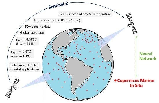
The aim of this work is to obtain high-resolution values of sea surface salinity (SSS) and temperature (SST) in the global ocean by using raw satellite data (i.e., without any band data pre-processing or atmospheric correction). Sentinel-2 Level 1-C Top of Atmosphere (TOA) reflectance data is used to obtain accurate SSS and SST information. A deep neural network is built to link the band information with in situ data from different buoys, vessels, drifters, and other platforms around the world. The neural network used in this paper includes shortcuts, providing an improved performance compared with the equivalent feed-forward architecture. The in situ information used as input for the network has been obtained from the Copernicus Marine In situ Service. Sentinel-2 platform-centred band data has been processed using Google Earth Engine in areas of 100 m × 100 m. Accurate salinity values are estimated for the first time independently of temperature. Salinity results rely only on direct satellite observations, although it presented a clear dependency on temperature ranges. Results show the neural network has good interpolation and extrapolation capabilities. Test results present correlation coefficients of 82% and 84% for salinity and temperature, respectively. The most common error for both SST and SSS is 0.4 °C and 0.4 PSU. The sensitivity analysis shows that outliers are present in areas where the number of observations is very low. The network is finally applied over a complete Sentinel-2 tile, presenting sensible patterns for river-sea interaction, as well as seasonal variations. The methodology presented here is relevant for detailed coastal and oceanographic applications, reducing the time for data pre-processing, and it is applicable to a wide range of satellites, as the information is directly obtained from TOA data.

1. Introduction

Covering around 71% of the Earth’s surface, oceans play a major role in the global climate system, [1]. The study of sea surface temperature and salinity is important to understand how oceans communicate with land and atmosphere, but also for the understanding of marine ecosystems and weather prediction, [2]. Sea surface salinity (SSS) and temperature (SST) are also relevant in the study of estuarine processes (mixing of fresh and sea water), stratification, hypoxia, organic matter, or algal blooms, among others, [3]. The SSS and SST data collection has typically been done by means of static buoys, drifters, and ship-based systems, [4]. The problems that these measurements present are related to poor extended data coverage. Moreover, the estimation of SST and SSS near the coast, where the detail needed might be higher due to the development of different near-shore processes and human activities, is difficult.

Different satellite missions have focused over the past decades on the measurement of oceanographic characteristics to overcome the issues that the in situ measuring techniques present. Satellites provide worldwide coverage of ocean and land phenomena, which is particularly relevant for the extraction of time series and general trends, but also for the study of localised events. One of these satellite operations is the European Space Agency’s (ESA) SMOS (Soil Moisture Ocean Salinity) mission, which provides measurements of both soil moisture and ocean salinity by using a Microwave Imaging Radiometer with Aperture Synthesis (MIRAS), [5]. The spatial resolution is 35 km at the centre of the field of view. On the other hand, NASA’s Aquarius mission focuses also on sea surface salinity from space, [6]. Its spatial resolution is 150 km.

The MODIS–Aqua mission (Moderate Resolution Imaging Spectroradiometer), [7], views the complete Earth’s surface every 2 days, obtaining information in 36 spectral bands. It started operations in 2000, and its role is relevant in the development of Earth system models. Bands capture information useful for the study of aerosols boundaries and properties, ocean colour, phytoplankton and biochemistry, water vapour, temperature, and much more. Data is acquired in three different spatial resolutions: 250 m, 500 m and 1000 m, having the bands used for ocean reflectance the latter. MODIS data has been used for the extraction of SST datasets.

Other sensors, such as SeaWiFS (Sea-Viewing Wide Field-of-View Sensor) [8], have been used for the extraction of SSS data from their colour information. It was designed to collect ocean biological data, mainly chlorophyll, and was active from 1997 to 2010. It recorded information in eight bands and its resolution ranges from 1100 to 4500 m. Moreover, the NOAA CoastWatch mission, [9], derived SST products from different instruments in a set of satellites: Visible Infrared Imaging Radiometer Suite (VIIRS) in the Joint Polar Satellite System, Advanced Very High Resolution Radiometer (AVHRR) in the MetOp, or Advanced Baseline Imager (ABI) from GOES-16, among others. In every case, the highest available resolution is in the order of 1000 m. The low available resolution in built-for-purpose ocean observation satellites is clear from the information provided above. This influences the use of remote data for coastal and detailed oceanographic applications, where more detail might be needed. The different satellite missions and principal characteristics detailed in this introduction are summarised in

Table 1. Summary of satellite missions and projects used for SST and/or SSS estimation.

Mission/Project	Measured Property	Sensor Type	Spatial Resolution	Revisit Time	Organisation
SMOS	Soil moisture, ocean salinity	MIRAS	35 km	3 days	ESA
Aquarius	Ocean salinity	Radiometer	150 km	7 days	NASA
MODIS–Aqua	Ocean colour and temperature	Spectro–radiometer	1 km	2 days	NASA
SeaWiFs	Ocean salinity	VNIR	1.1 km	2 days	NASA
Sentinel-2	Coastal areas and water bodies monitoring	Multi-spectral	60 m	5 days	ESA
Sentinel-3	Ocean colour	Radiometer and spectrometer	300 m	2 days	ESA
CoastWatch	Ocean temperature	VIIRS, AVHRR, ABI, ...	1 km	-	NOAA

.

SST is normally estimated from satellite measurements following different retrieval algorithms, depending on the type of sensor. For example, [10] summarises the SST retrieval algorithm for Aqua. This is based in the correction of several factors affecting temperature at the surface, leading to an accurate estimation of SST through clouds. The corrections included in the algorithm are due to atmosphere, wind, incident angle, sea ice, sun glitter, land contamination, salinity, and ground interferences. The inclusion of corrections leads to higher SST-derived accuracy. The spatial resolution of the satellites considered in [10] is about 50 km. Moreover, [11] evaluates the accuracy of SST at different frequencies. It is found that radiometer noise and geophysical errors are less representative in lower frequencies and are independent of latitude.

Although some satellite data provide users with direct SST information and retrieval algorithms, researchers are developing techniques to further estimate SST information and make more accurate predictions. The use of neural networks to estimate oceanographic information is a good example of further efforts in predicting SST. [12] presents an artificial neural network model to predict SST based on measurements of SST in the previous day. A 2-year dataset is predicted with errors below 0.5 °C in most cases. [13] predicts SST in the western Mediterranean Sea using in situ data to train the neural network: sea level pressure, wind components, air temperature, dew point temperature, and total cloud cover. A total of 45 years of data are provided, and these are combined with satellite-derived SST data from Pathfinder and MODIS at a resolution of 4 km. The neural network provides accurate predictions of seasonal and interannual SST variability, and the methodology is then used to reconstruct incomplete SST satellite images.

The method proposed in [14] combines numerical estimations with SST measurements to produce real-time SST in the Indian Ocean using a wavelet neural networks. NOAA’s AVHRR SST derived data is used in this study together with other remotely obtained information, linked to numerical data provided by the Indian National Centre for Ocean Information Services (INCOIS). The results provide accurate daily, weekly, and monthly SST values. Finally, some innovative techniques have compared the SST obtained by using AVHRR information and with data collected by surfers, [15]. However, the resolution of the AVHRR is around 1 km. While this is useful for oceanographic applications offshore, more detail is needed near the coast for specific applications.

Looking now into sea surface salinity estimation, the amount of literature in this area is less extensive than that for SST. In the last decades, different research projects have focused on the extraction and validation of SSS from the information provided by satellites, and have combined this with the use of machine learning techniques. [16] investigates the ability of two algorithms (least squared and second polynomial order) to retrieve SSS from MODIS satellite data. The information is compared with in situ data from the South China Sea. They found out that the least square algorithm can be used to retrieve SSS from MODIS data. In line with this, other studies have given a step further, and implemented neural networks to predict SSS. [17] uses 9000 salinity records from four research vessels matched with MODIS–Aqua satellite data to train a neural network that estimates SSS in the mid-Atlantic area, obtaining relevant values for estuarine areas.

In a further step, [3] developed a neural network to estimate SSS in the Gulf of Mexico. This study uses ocean reflectance data reprocessed by NASA from MODIS–Aqua and SeaWiFS data, and the resolution is in the range of 1000 m. The satellite information includes atmospheric correction, and the time window allowed to match in situ and satellite data is ±6 h. Other studies present interesting approaches to solving the salinity characterisation issue: [18] presents a 6-year study on the salt distribution in the Western Mediterranean Sea from SMOS information, reducing errors from previous studies. The study is based in the use of debiased non-Bayesian retrieval Data Interpolating Empirical Orthogonal Functions (DINEOF), and multifractal fusion. Both the North Atlantic and Mediterranean Sea are mapped using this technique, providing reduced error in SMOS SSS. The different methodologies described in this section are summarised in

Table 2. Summary of satellite missions and projects used for SST and/or SSS estimation.

Estimated Property	Method	Notes	Location
SST [10,11]	Retrieval algorithm for MODIS–Aqua	Very low resolution (50 km). Noise and geophysical errors more representative in higher radiometric frequencies.	Worldwide
SST [12,13]	NN from previous days info/from relevant meteorological components	Low resolution (4 km). Long-term data needed (45 years). Localised results.	Indian Ocean/Western Mediterranean Sea
SST [14]	NN from numerical model	Very low resolution (20 km). Combines numerical and neural techniques. Focuses on error time-series.	Indian Ocean
SST [15]	AVHRR-derived compared with local information	Low resolution (1 km). Dependent on limited in situ data sources. Innovative approach to mitigate drawbacks from remote sensed information.	North-East Atlantic Ocean
SSS [16]	Algorithm from MODIS data	Low resolution (1 km). High accuracy of algorithm tested.	South China Sea
SSS [17]	MODIS–Aqua, neural network	Low resolution (1 km). Relevant for estuarine processes. Relatively high errors. Relationships between SST and SSS.	Mid-Atlantic Ocean
SSS [3]	NN MODIS and SeWiFs.	Low resolution (1 km). Match in situ-satellite range ±6 h. Site-specific.	Gulf of Mexico
SSS [18]	SMOS-derived (6 years), data interpolation.	Improved resolution (SMOS), but still low for coastal applications (5 km). Error-reducing. High accuracy compared to in situ data.	Western Mediterranean Sea and North Atlantic Ocean.

.

Reference [19] recently presented an article on the extraction of ocean salinity from space. The paper presents the difference in development of the satellite-observed salinity missions and developments compared with sea surface temperature, which has been done for the past four decades. The paper states the requirement of using temperature in order to estimate salinity, as temperature impacts the brightness temperature of the ocean observed from space. In contrast, the research presented in the following sections shows how salinity can be estimated without the need of including temperature as input.

For the purpose of this study, generic optical satellite information has been chosen: ESA’s Sentinel-2 Level 1-C. As pointed out previously, there are built-for-purpose satellite missions which focus on the observation of ocean colour, such as Sentinel-3, [20], or NASA’s MODIS–Aqua, [7]. However, Sentinel-2 allows to produce higher resolution SSS and SST datasets from its 10–60 m band resolutions (compared with the 300 m from Sentinel-3, and 1000 m for MODIS–Aqua). Moreover, we include band and general image information, in order for the network to learn atmospheric relationships, such as cloud coverage, water vapour, or mean angle of incidence. The in situ information has been obtained from the Copernicus Marine Environment Monitoring Service (CMEMS), which has been operational since May 2015. This is part of the Copernicus programme, which is an initiative from the European Union for the establishment of a European capacity for Earth Observation and Monitoring, [4]. Copernicus is composed of three components: Space, Insitu, and Services. The first one includes the European Space Agency’s (ESA) Sentinels, as well as other contributing missions operated by national or international organisations. The Insitu component collects information from different monitoring networks around Europe, such as weather stations, ocean buoys, or maps. This information is key to calibrate and validate satellite data.

Taking into account the research done in the area, in the present paper, we aim at obtaining SST and SSS from TOA data, thus developing a methodology that reduces the amount of pre-processing needed from the satellite data, such as atmospheric corrections. Moreover, the use of optical satellite data provides a wide variety of options where the proposed methodology is applicable. Special attention is paid to the use of raw data, allowing wider use and faster extraction of information. Moreover, the time window between in situ measurement and equivalent satellite image has been reduced in this paper to 1 h, which is considerably lower than that used in previous research papers. The reduced time window linked to the high resolution provided by Sentinel-2, provides higher reliability than previous methodologies. Moreover, this research allows the prediction of sea surface salinity independently of sea surface temperature, based on the hypothesis that the neural network is built with enough information to obtain key salinity relationships with visual parameters.

The paper is composed of three main sections, and is structured as follows: Section 2 presents the methodology followed in the paper, including extraction of in situ and satellite data, matching process, data usage and coverage, and neural network details. Section 3 includes the discussion of prediction results for sea surface temperature and salinity in interpolation and extrapolation problems, as well as a sensitivity analysis, and neural network evaluation over a region of interest. Finally, Section 4 presents the work conclusions.

2. Methodology

In this section, the main considerations taken into account in the selection of in situ and satellite information are summarised, as well as the matching process followed to correlate physical observations with remote ones. After that, the set up parameters of the neural network used to estimate SST and SSS from satellite information are described.

2.1. In Situ Data

In situ data from the Global Ocean, Arctic Ocean, Baltic Sea, European North-West Shelf Seas, Iberia–Biscay–Ireland Regional Seas, Mediterranean Sea, and Black Sea have been collected for the purpose of this paper. The data has been obtained from Copernicus Marine In Situ, [4]. Two types of datasets are provided in the Copernicus in situ component. The Reprocessed (REP) dataset is processed and validated, and thus delivered in delayed mode, which means that the information is updated on a yearly basis. On the other hand, the Near-Real-Time (NRT) dataset is provided nearly instantaneously, but the level of preprocessing is minimal, accounting for higher uncertainties. The in situ delayed mode product is designed for reanalysis purposes, and integrates the best available version of in situ data for SST and SSS measurements, [21,22]. These data are collected from ICOS Ocean Thematic Centre operational stations, using Standard Operating Procedures for the ocean carbon community.

The NRT product is updated with new observations at a maximum frequency of once a day, depending on the connection capabilities of the platform, [21]. REP products integrate the best available version of in situ data for temperature and salinity measurements, [22]. These data are collected from main global networks (Argo, GOSUD, OceanSITES, World Ocean Database) completed by European data provided by EUROGOOS regional systems and national system by the regional in situ components. It is updated on a yearly basis. The products are delivered by authenticated FTP. Individual automatic tests and statistical tests are performed to the data. When the data is doubtful, visual control by ocean experts is done, [22]. As a result, quality control flags are assigned to the measurements, and provided with the product. The temporal coverage ranges from 1990 until 2018. Both NRT and REP products are used in this paper to have the most up to date repository, and filtered to avoid duplicates.

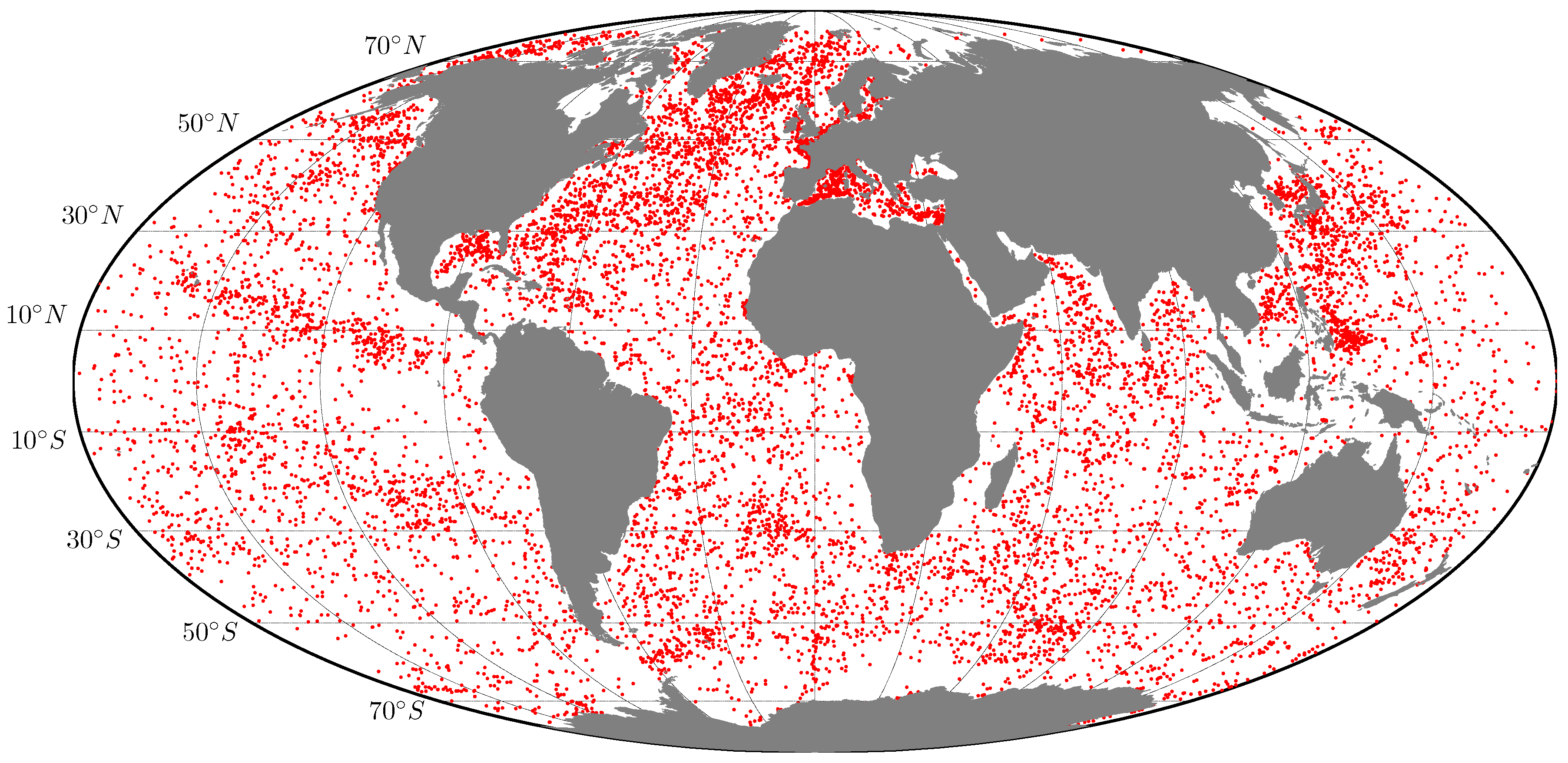
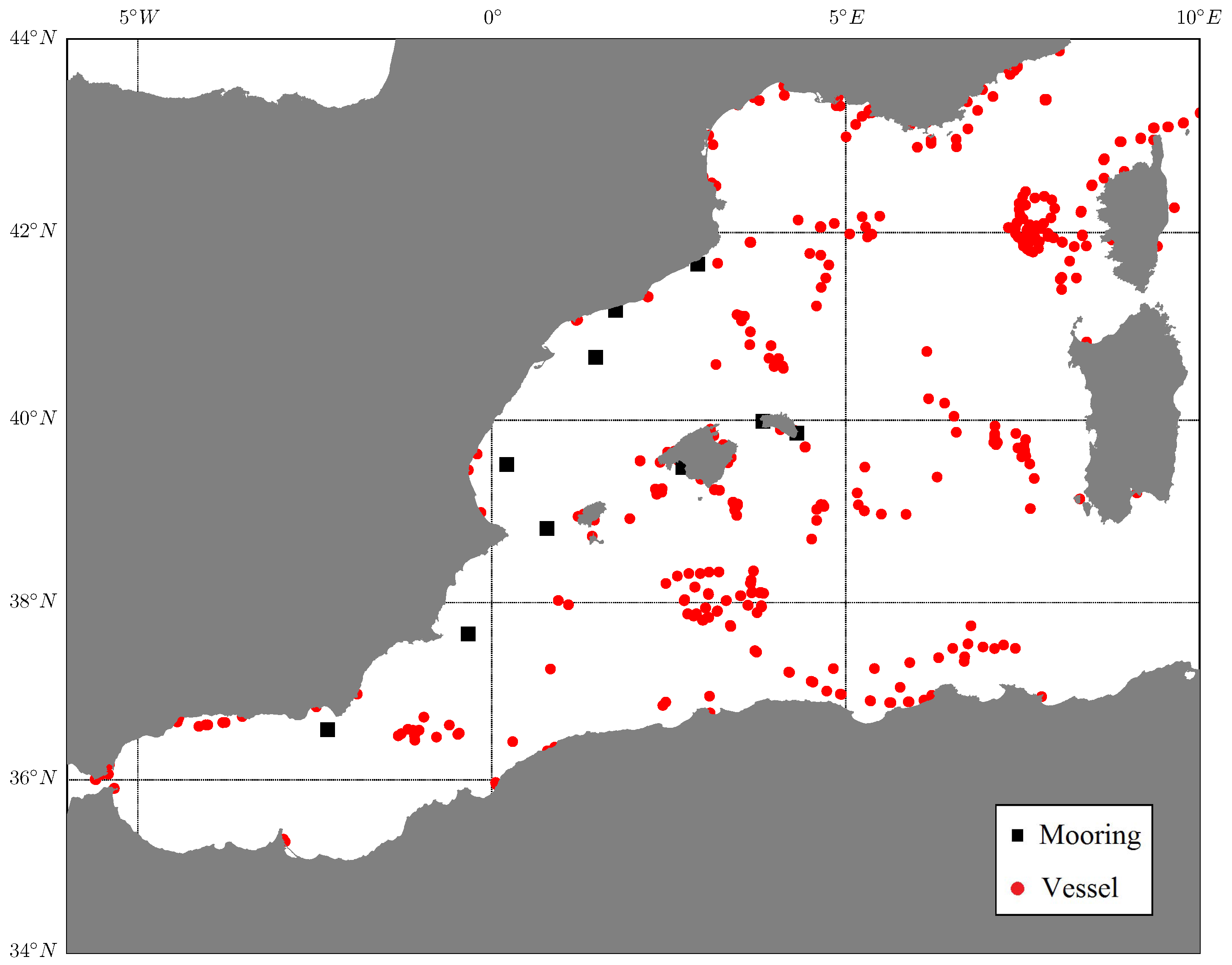
There are more than 14,000 platforms worldwide with available data from 2015 (the coverage period of Sentinel-2), and taking only platforms with salinity and temperature, that number reduces to around 4600, see Figure 1. Due to the amount of information, it is not possible to provide the detail of all the platforms, but as a detailed example, a list of the mooring platforms in the Western Mediterranean Sea is provided in

Table 3. Example subset of reprocessed in situ mooring observations obtained from [22] in the Western Mediterranean Sea. The columns represent (from left to right): the official name of the dataset in the Copernicus Marine registry, latitude and longitude of the platform location, name of the closest city or region, water depth in that point (z), distance to nearest shore (d), and number of observations matching satellite data from 2015 (#).

In Situ Observation	(Lat, Lon) (${}^{\circ }$)	Location	z (m)	d (km)	#
Off-shore buoys
MO_TS_MO_61141	($38.82$, $0.78$)	Ibiza	800	$34.3$	40
$IR\_TS\_MO\_61198$	($36.57$, $-2.32$)	Cabo de Gata (Almeria)	536	$19.7$	188
$IR\_TS\_MO\_61280$	($40.68$, $1.47$)	Tarragona	688	$51.4$	178
$IR\_TS\_MO\_61281$	($39.52$, $0.21$)	Valencia	260	$46.1$	143
$IR\_TS\_MO\_61417$	($37.65$, $-0.33$)	Cabo de Palos (Cartagena)	230	$33.6$	210
Near-shore buoys
$MO\_TS\_MO\_61499$	($39.49$, $2.70$)	Mallorca	30	$2.5$	77
MO_TS_MO_LA-MOLA	($39.86$, $4.31$)	Menorca (East)	10	$0.36$	13
MO_TS_MO_SON-BLANC	($39.99$, $3.83$)	Menorca (West)	6	$0.08$	29
$MO\_TS\_MO\_OOCS$	($41.67$, $2.91$)	Gerona	192	$3.9$	38
$MO\_TS\_MO\_OBSEA$	($41.18$, $1.75$)	Barcelona	20	$3.2$	318
Total					1234

(please note that the number of observations represent those that have matching satellite data). For each platform, SST and SSS have been obtained. Moreover, a map marking the points where the specific buoys are located is given in Figure 2.

2.2. Satellite Data

Sentinel-2 satellite data has been used for the purpose of this paper, [23]. Sentinel-2 is a multi-swath, high-resolution, multi-spectral imaging mission supporting Copernicus Land Monitoring studies including, among others, the observation of coastal areas. Level 1-C contains 13 spectral bands representing TOA reflectance without any kind of atmospheric correction. Its revisit interval is 5 days. Sentinel-2 offers a resolution of $10$ m in the colour bands, going up to $60$ m in others, such as water vapour or aerosols bands. The information has been processed and downloaded using Google Earth Engine, [24]. Google Earth Engine is an integrated cloud-based platform for geospatial analysis that provides Google’s computational capabilities, which allows processes that would take hours to run in a supercomputer, to run in seconds, [25].

The information used as input to the neural network is raw data extracted from the satellite band information and tile properties, see

Table 4. Sentinel-2 band information used in this study, obtained from [24]. (*) Band QA60 has not been used as input for the Neural Network.

Data	Resolution (m)	Wavelength (nm)	Description
B1	60	443.9	Aerosols
B2	10	496.6	Blue
B3	10	560	Green
B4	10	664.5	Red
B5	20	703.9	Red Edge 1
B6	20	740.2	Red Edge 2
B7	20	782.5	Red Edge 3
B8	10	835.1	NIR
B8a	20	864.8	Red Edge 4
B9	60	945	Water vapour
B10	60	1373.5	Cirrus
B11	20	1613.7	SWIR1
B12	20	2202.4	SWIR2
QA60 (*)	60	-	Cloud mask

and

Table 5. Other information used in this study from Sentinel-2, obtained from [24].

Data	Description
Cloud pixel percentage	Granule-specific cloudy pixel percentage.
Cloud coverage assessment	Cloudy pixel percentage for the whole archive.
Mean Incident Azimuth angle for every band ($\times 13$)	Mean value containing viewing incidence azimuth angle average for each band.
Mean Incident Zenith angle for every band ($\times 13$)	Mean value containing viewing incidence zenith angle average for each band.
Mean Solar Azimuth angle	Mean value containing sun zenith angle average for all bands.
Reflectance conversion correction	Earth-Sun distance correction factor.

. By providing all remote available information to the network, we expect it to infer the sea surface temperature and salinity without atmospheric corrections or any other type of band preprocessing.

2.3. Matching Process

The in situ data download has been done using Python-programmed access to the Copernicus Marine FTP service. Data processing and matching with Sentinel-2 data have been done by means of Google Earth Engine, [24]. This has been done entirely by using Python thanks to the Earth Engine Python API. The process to match the data is as follows:

• In situ data containing salinity and temperature from the 23 June 2015 onwards (start of Sentinel-2 mission) is downloaded from the Copernicus Marine In Situ data portal, [4]. Data worldwide is obtained, with more than $\mathrm{11,000}$ files and about 160GB of data downloaded.
• For each in situ measurement point, the Sentinel-2 image collection is filtered to the tiles that contain the point on the day and time when the measurement was taken. The image is only considered if the in situ measurement was taken within 1 h of Sentinel-2 pass time. Previous research considered wider time windows, but with this approach more accurate results are expected.
• If there is any valid tiles for that point, they are clipped in boxes of $100$ m $\times 100$ m area centred in the point location to obtain high-resolution estimators of SST and SSS. This box size is taken to average the effect of wave reflectance.
• For each box, the properties and band data summarised in Table 4 and Table 5 are extracted by Reducing the properties in the box. The Reducer used is the mean value. The Reduction technique is a way to aggregate data over space in Earth Engine, applying statistics over a wide range of information.
• The time difference between the in situ measurement and the satellite image is recorded. In case of multiple tiles covering the point of interest, the matched data is sorted by time difference, and the one with the smallest difference is selected.
• A table containing satellite data (band information and other properties) and equivalent in situ information (salinity and temperature) for each valid point is composed.
• Band QA60 containing a cloud mask has been used to select points only with a clear sky, i.e., points were clouds are persistent have not been considered: no opaque clouds or cirrus clouds present.

2.4. Data Usage and Coverage

Worldwide, there are a total of 9695 valid points from an initial batch of $64,672$ points with information within 1 h of the passing time of Sentinel-2 and without clouds. Please note that the initial $64,672$ points have been already pre-filtered using the data quality check process provided by Copernicus, only selecting data with the highest level of accuracy (quality flag QC1 only). If we consider the reduction of information when taking into account clouds, if cirrus clouds where considered, we had a reduction of $64672\to 22286$, about $66\%$ less data. Taking away all types of clouds, we reduce the amount of information to 9695 points, about $85\%$ reduction from the initial batch of data. The authors would like to point out how extensive the cleaning of data has been to obtain the final input information for the neural network. As an example of the data distribution, as shown in Table 3, for the Western Mediterranean there are a total of 1234 matching observations, which represents $13\%$ of the total used data due to the lack of clouds in that area.

2.5. Neural Network

As presented in the introduction, artificial neural networks have been used in the recent years in combination with Ocean Observation techniques to improve the available information and develop new products. Neural networks are a programming paradigm inspired by biology, [26], and they allow computers to “learn” from observed data. In this paper we refer to Deep Neural networks, which are a specific set of atificical neural networks. These have been successfully used in image recognition, speech recognition and language processing. Neural networks can be used for regression problems as the one presented in this paper. In [27], different network architectures are presented for the specific regression problem. Here we focus on deep feed-forward networks.

SST and SSS in situ information is used as ground truth for the neural network scheme. In other words, estimated SST and SSS will be the outputs of the neural network, while the inputs will be the satellite parameters summarised in Table 4 and Table 5. The estimated SSS and SST are compared with their equivalent in situ values. When building the network, latitude and longitude of the observations have not been included as input variables to ensure the network independence from location (i.e., the network could learn patterns for certain locations). Same process has been followed for the time of the year when the measurement was taken. Note also that as commented in previous sections, salinity has been obtained solely on direct satellite observation, and SST values have not been provided to estimate salinity. Previous works presented the need to include SST in order to accurately estimate SSS, [19]. That barrier has been overcome in the present paper. The hypothesis underlying this feature is that the band data provided to the network contains enough information to extract salinity, as temperature is also being obtained with those same inputs. In other words, if the network is able to predict temperature, given those same parameters it should be able to find the relationship between brightness temperature and salinity.

2.5.1. Data Processing, File Loading, Filtering and Outliers Removal

Files containing valid data points are loaded and filtered in terms of the cloud mask contained in band QA60. Duplicates are dropped to ensure the network is not fed with information defined multiple times. Outliers are removed by including minimum and maximum thresholds. The minimum threshold is defined as the mean of each input minus three times their standard deviation, and the maximum threshold is defined as the mean plus three times the standard deviation. We ensure that any values outside a range of six standard deviations are not considered in the network. The reason to choose this thresholding criteria for outliers is that assuming data follows a normal distribution, any data points in the tail of the distribution over three standard deviations from the mean represent about $0.1\%$ of the information, and is normally considered an outlier in statistics.

2.5.2. Normalisation

The data is normalised by using the following:

$$X_{norm}={\displaystyle \frac{X-X_{min}}{X_{max}-X_{min}}},$$

(1)

where $X_{norm}$ is the normalised value, X is the original value, $X_{min}$ is the minimum value of the normalised parameter list, and $X_{max}$ is the maximum value of the normalised parameter list. Minimum and maximum values are defined as the limits after the thresholding process described in the previous section to identify outliers. This type of normalisation is defined as the Min–Max Feature Scaling. Following this process, each variable will be within [0–1] limits, reducing weighting biases towards variables with bigger initial values.

2.5.3. Training and Test Data Split

Depending on the type of test performed on the data, it is split in a specific way. For interpolation (the network will infer information from a platform where partial information has been provided, e.g., estimating a buoy salinity and temperature in summer by training the network with data from that buoy in winter), data is shuffled to ensure it is distributed randomly. The training section is then selected as the first $90\%$ of the data, while the last $10\%$ is used to test the neural network. In the extrapolation problem (the network will infer information from a platform where no previous information is given, e.g., estimating a buoy salinity and temperature without having any previous information from that buoy to train the network), specific platforms are considered as test, and the rest of platforms are used to train the network.

The reasons to choose these scenarios assure that: (1) the neural network does not depend on the geographical location of buoys; and (2) the neural network is able to interpolate but also to extrapolate to conditions not previously seen. Within the training data, a $10\%$ is selected as validation data to check the convergence of the steps taken during training.

2.5.4. Trainer

Once data has been filtered split and normalised, the train starts. Relevant optimisers, loss functions and metrics are selected. The optimal weights are saved and used as model checkpoint. Early stopping is set when the training stops improving, and the learning rate is reduced on plateau. The layers are batch-normalised to reduce internal covariate shift [28].

2.5.5. Running Predictions

Once the neural network has been trained and the selected loss function has been optimised, the results are tested in the Test section of the data to check that the network is able to run predictions (interpolate or extrapolate, depending on the case faced). Statistical values are extracted from these predictions to check how well the network performed with the parameters selected.

2.5.6. Architecture of the Neural Network

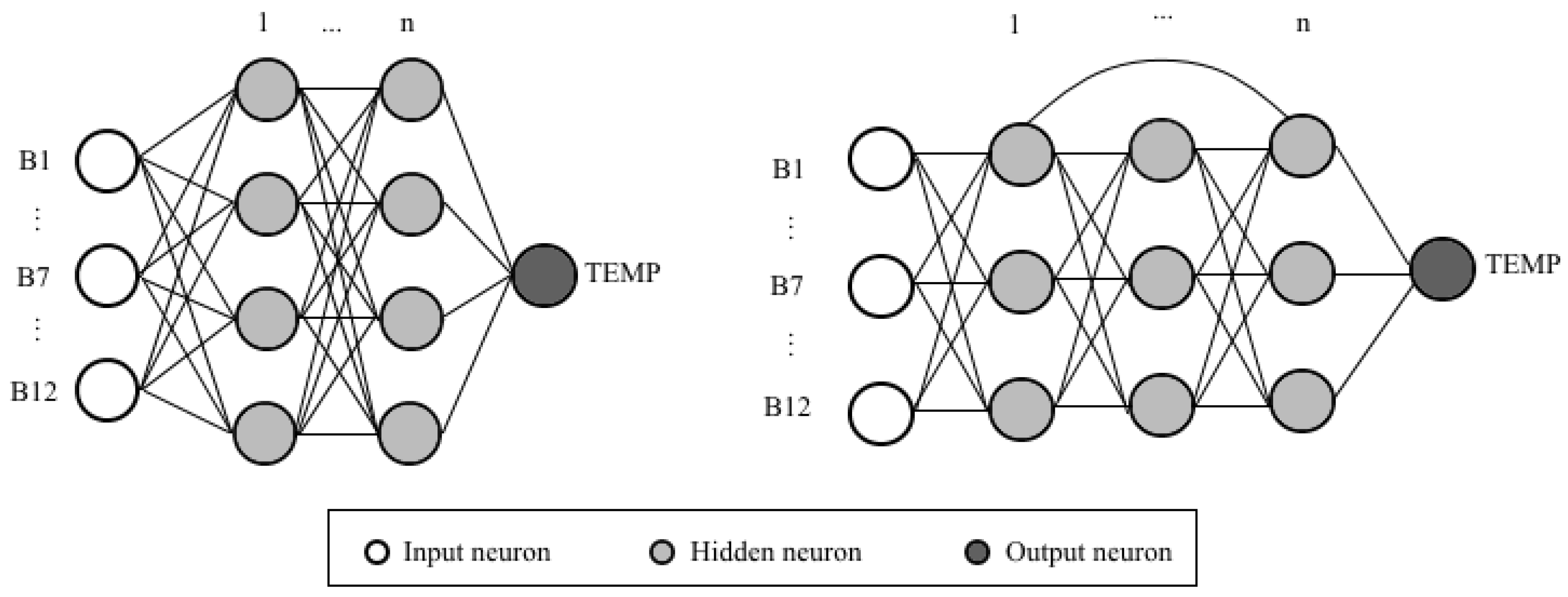
The input layer is composed of 43 variables equivalent to the items summarised in Table 4 and Table 5, combining band information and image properties. The 43 input variables are: Band data (B1, B2, B3, B4, B5, B6, B7, B8, B8a, B9, B10, B11, B12), Cloud pixel percentage, Cloud coverage assessment, Mean incident azimuth angle for each band (13 input values), Mean incident zenith angle for every band (13 input values), Mean solar azimuth angle, and Reflectance conversion correction. The output layer is single, either temperature or salinity. Please note that the two variables have been trained separately to prove that temperature is not needed to infer salinity from satellite observations. More than 100 network combinations, including different number of hidden layers, nodes, activation functions, regularization and optimisation techniques, have been tried for the purpose of this paper. The combination that provides the best results is composed of 20 hidden layers with 43 nodes in each layer. The activation function is tanh for every layer except for the output layer, where a sigmoid is used. Losses are calculated following a logcosh. The optimiser used is Adamax, and the network is batch-normalised.

The goal of a neural network is to estimate a function that connects inputs with outputs, [29]. They have an input layer where the initial information is provided, one output layer, where the variable that we want to infer is included, and may have multiple hidden layers with multiple neurons each to infer the relationship between inputs and outputs, see Figure 3. Shortcuts have been used in a second architecture to avoid the so called vanishing gradient problem, [30]. This is found when training neural networks with bacK-propagation, as every weight is updated depending on the partial derivative of the error in each iteration. In some cases this gradient will become smaller in each step, avoiding the change of the weight value. In extreme cases, this problem might stop the network from further training. Residual networks avoid this issue by skipping connections, or jumping layers, see Figure 3. By doing this, previous activations are re-used, adapting the weights of adjacent layers, [31]. Networks with shortcuts show an improved behaviour compared to the classical network.

The different activation functions tested in this research are the following:

-

ReLu:

$$f\left(x\right)=max(0,x)$$

(2)

-

Sigmoid:

$$f\left(x\right)={\displaystyle \frac{1}{1+e^{-x}}}$$

(3)

-

Tanh:

$$f\left(x\right)={\displaystyle \frac{e^x-e^{-x}}{e^x+e^{-x}}}$$

(4)

where x is the input to the layer, and $f\left(x\right)$ is the output to the next layer. The loss functions tested are defined below:

-

Mean Absolute Error:

$$MAE={\displaystyle \frac{1}{n}}\sum _{j=1}^n|y_j-{\widehat{y}}_j|$$

(5)

-

Mean Squared Error:

$$MSE={\displaystyle \frac{1}{n}}\sum _{j=1}^n{(y_j-{\widehat{y}}_j)}^2$$

(6)

-

Logcosh

$$L=\sum _{j=1}^{n}log\left(cosh(y_j-{\widehat{y}}_j)\right)$$

(7)

where n is the number of observations, $y_j$ is the ground truth, and ${\widehat{y}}_j$ is the predicted variable. Different combinations of the activation functions and losses have been used to obtain the optimal performance of the neural network.

3. Results and Discussion

In this section results are presented and discussed. Interpolation is first presented showing temperature and salinity results. Extrapolation results for specific platforms that have not been used to train the network are shown afterwards.

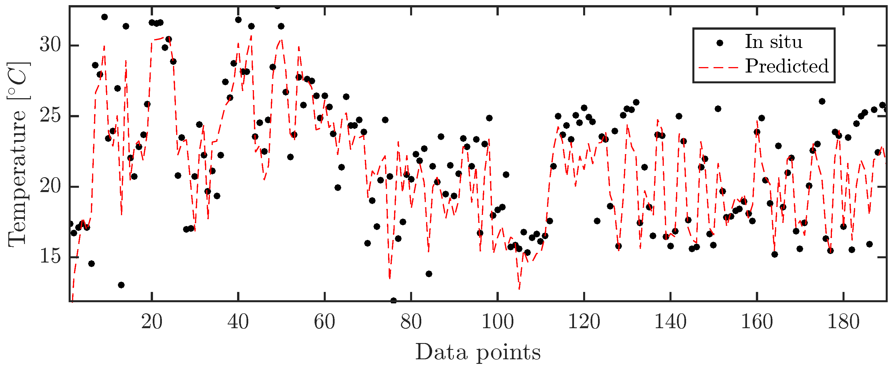
3.1. Temperature Interpolation

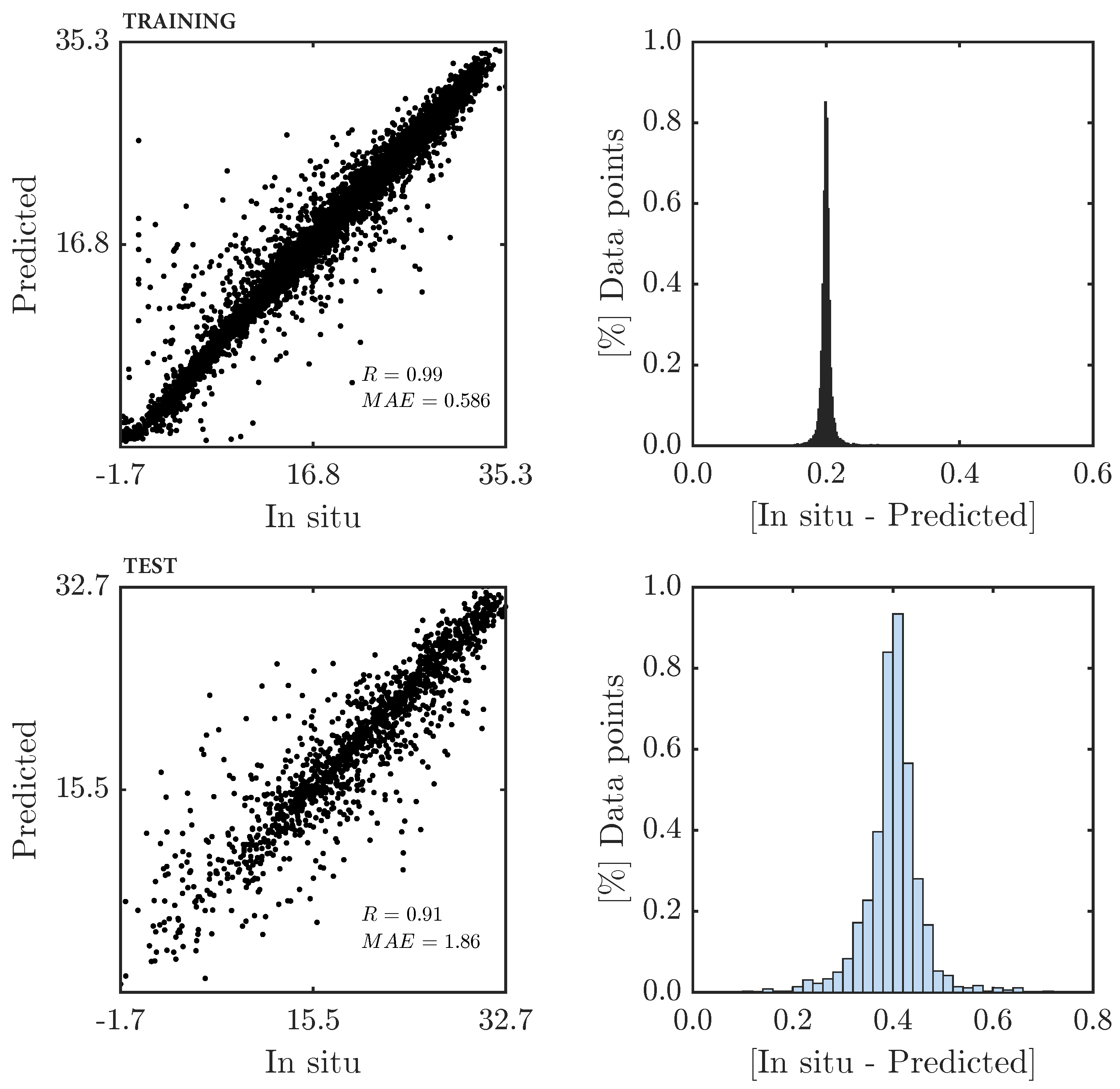
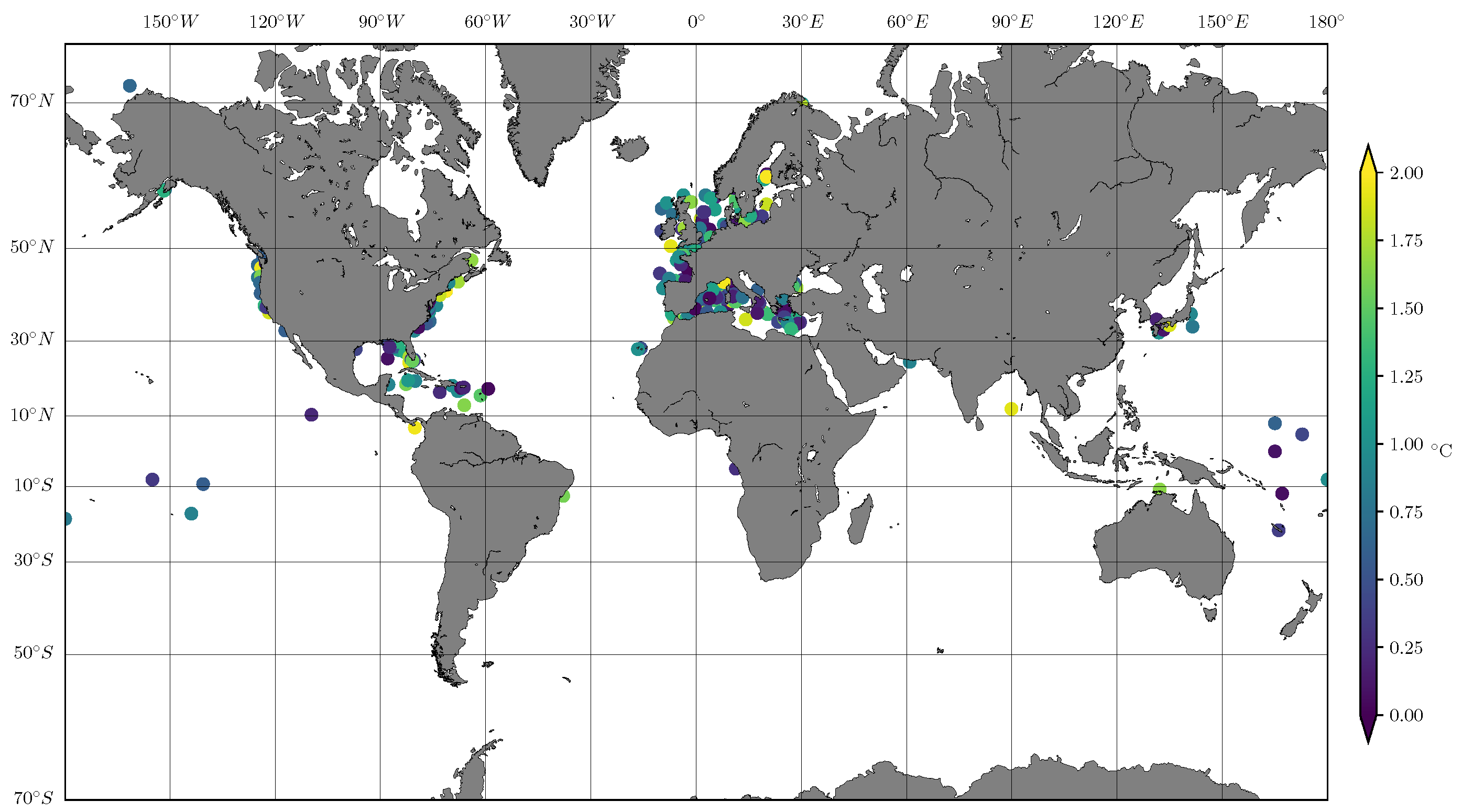
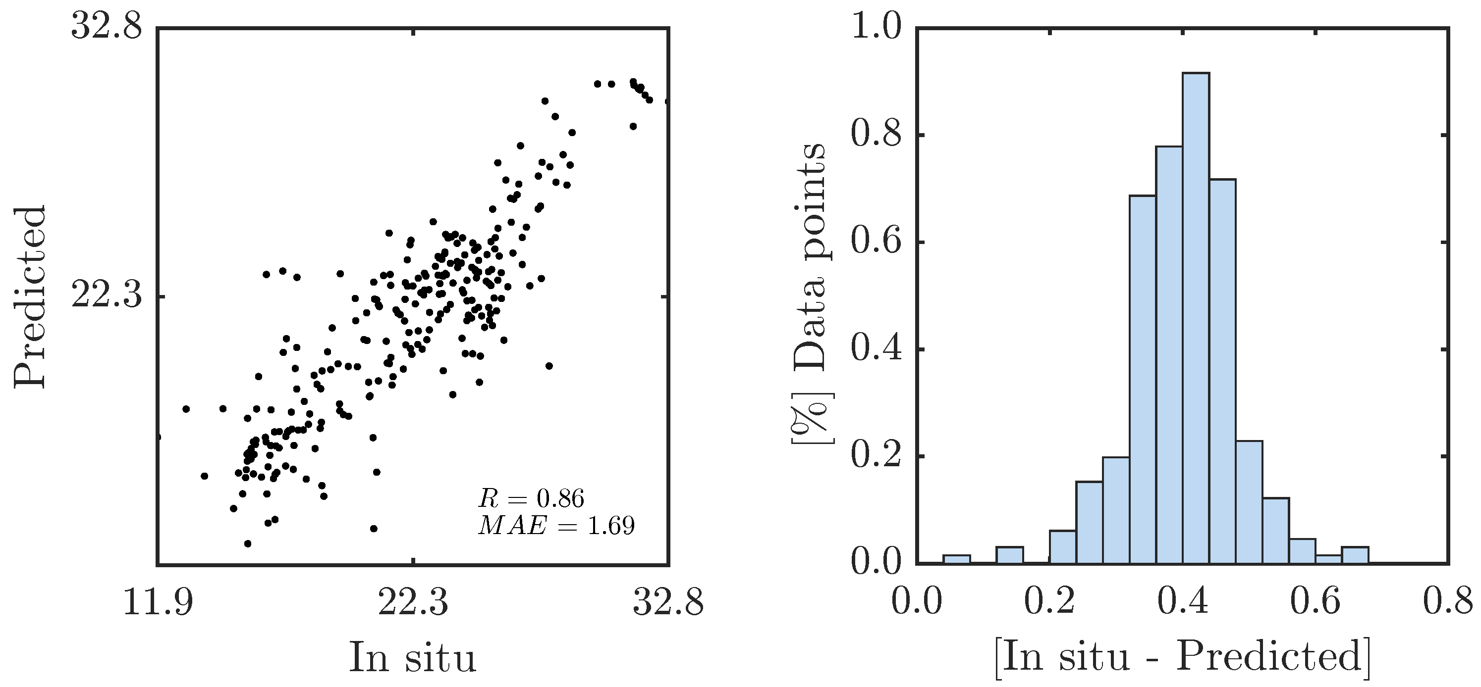
Figure 4 shows temperature interpolation for a random $10\%$ of the data. The test data is shown in the bottom panel, together with the variation between expected and estimated data in a colour scale. The goodness of fit is calculated using the Pearson correlation coefficient R and the mean absolute error ($MAE$). $MAE$ is defined in Equation (5), and R is defined as follows:

$$R={\displaystyle \frac{E\left[(\widehat{y}-{\mu }_{\widehat{y}})(y-{\mu }_y)\right]}{{\sigma }_{\widehat{y}}{\sigma }_y}}$$

(8)

where E is the expectation, y is the ground truth variable, $\widehat{y}$ is the estimated variable, $\mu$ is the mean and $\sigma$ is the standard deviation. R can take any value from −1 (total negative correlation) to 1 (total positive linear correlation), with $R=0$ meaning no correlation between the studied variables.

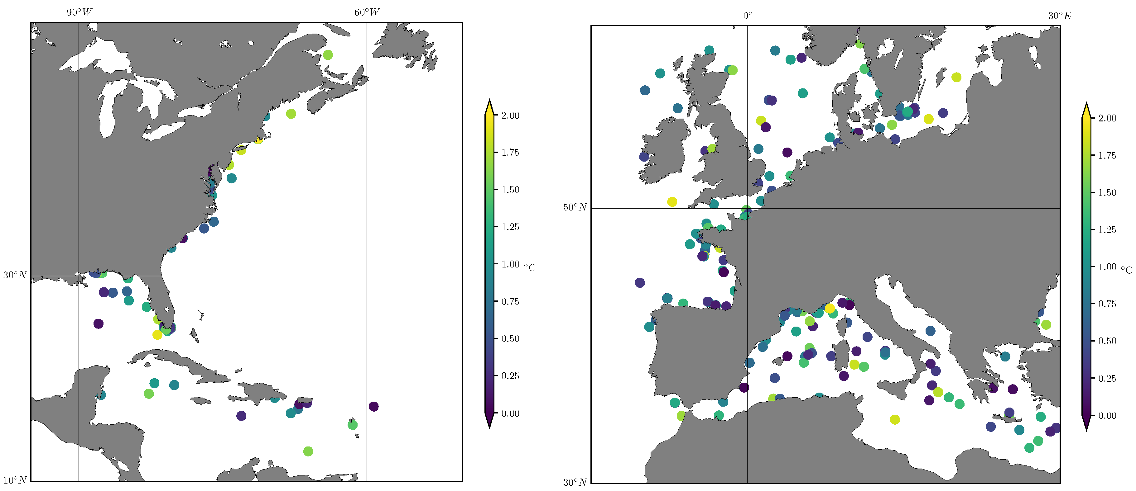
The test dataset is mainly located around Europe and North America, with some points around the Caribbean and Polynesia. Correlation values are over $90\%$ in both training and test sets, showing a very good agreement between predicted and expected data. MAE is below 1.9 ${}^{°}$C for the test dataset. Residuals are centred around 0.4 ${}^{°}$C, which is the most common error in the test dataset for more than $90\%$ of the data. This result linked to the MAE shows how most of the data is fitted well, but there are some outliers that differ significantly from the expected value, modifying the mean error. Looking at the distribution of errors around Europe in Figure 5, most of the values around the French coast, English Channel and North Sea show a very good agreement with errors below 0.5 ${}^{°}$C, while the Mediterranean has some outliers reaching 1.5 ${}^{°}$C in some points near Marseille. Otherwise, a good agreement is also observed in this area. In the US coast, agreement is also good.

3.2. Salinity Interpolation

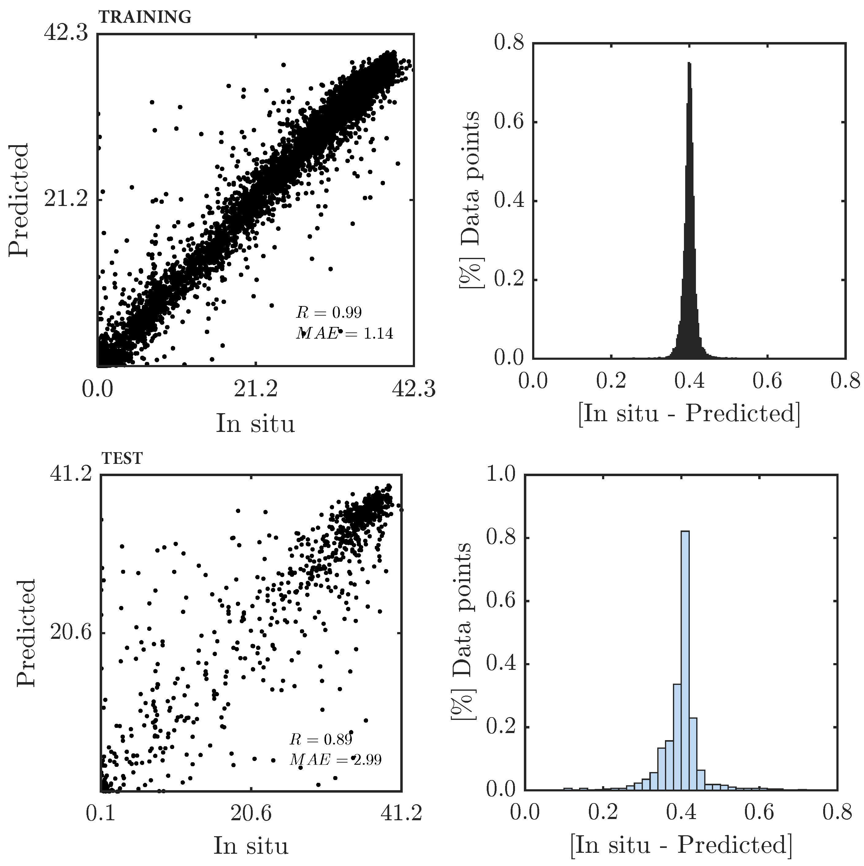
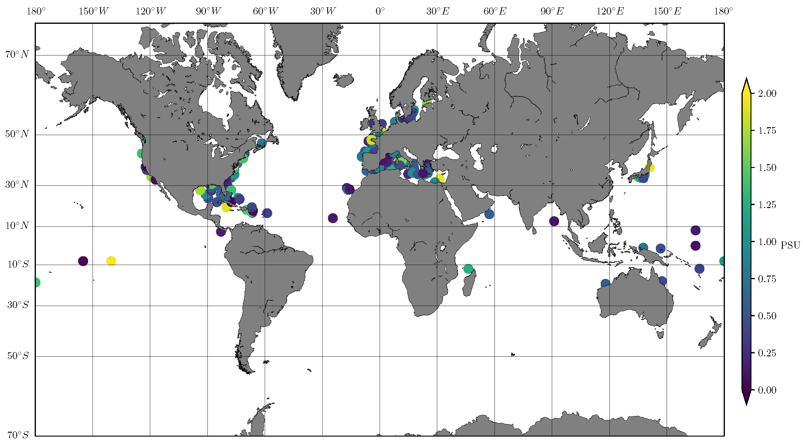
Salinity interpolation shows poorer results than their temperature equivalents. Most of the randomly selected test data is located in the Mediterranean and in the west and east coasts of the US, with some points around the Canary islands, Oman and Australia. In this case, test correlation reaches $89\%$, with a mean absolute error of 3 PSU, while the most common error lies around 0.4 PSU, Figure 6. As in the case of temperature, the most common difference is very good, but the existence of outliers makes the mean error increase significantly. The methodology followed in this paper takes into account an area of $100\times 100$ m around the in situ measurement location, providing an averaging on reflection conditions or sea foam. However, the presence of other factors at a bigger scale, such as algae patches, vessels, or other external features in the surroundings could affect the final value used as input to the neural network. Outliers are observed to be randomly located and isolated, and thus the presence of external features altering the averaging value of the region around the measurement point could be the cause for the existence of outliers in the prediction capability of the network. Another possible reason is linked to the fact that in situ measuring devices are not perfectly calibrated, and that can lead to a mismatch between observation and prediction. However, given that these instruments have been monitored and checked by different systems, this reason is unlikely to be the cause of outliers in the prediction.

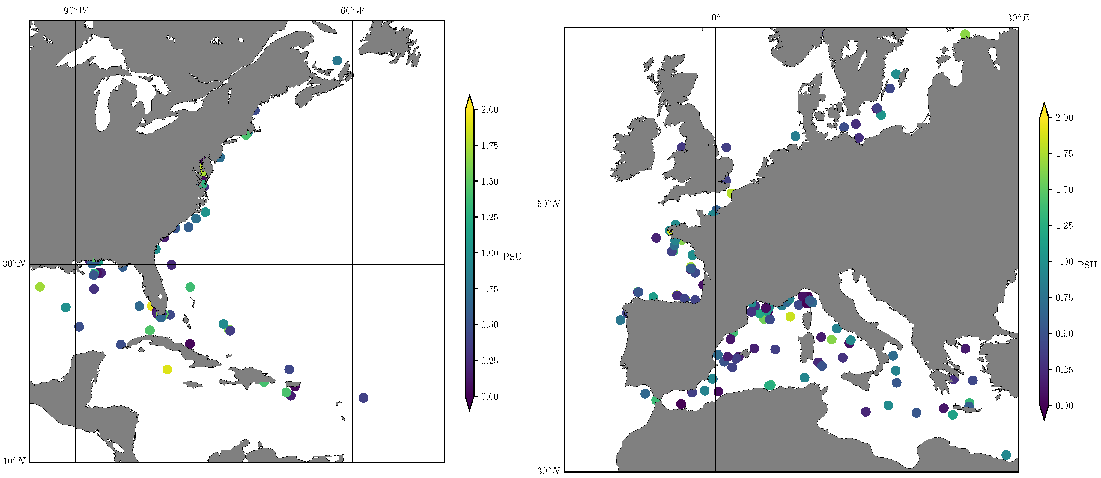
Focusing on the zoomed results provided in Figure 7 around the US east coast and Europe, the agreement in the Mediterranean is very good, with most of the results showing errors below 0.5 PSU. The points around the US also show very good agreement, with localised outliers in the Gulf of Mexico and below Cuba.

Dependence on Temperature Ranges

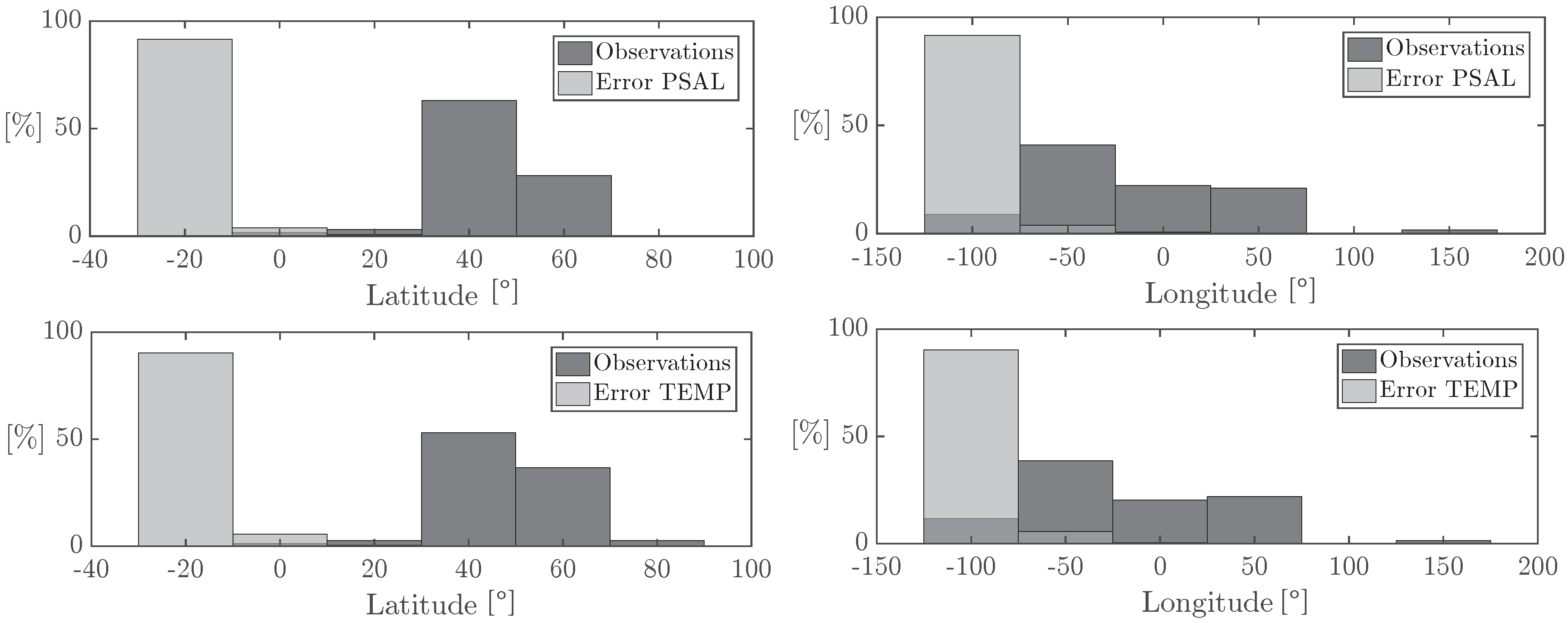
Although salinity was estimated independently of its temperature counterpart, a clear dependency was observed with temperature values in the training set. The accuracy of salinity estimations in the test set for areas with temperatures below 10 ${}^{°}$C is poor, as presented in

Table 6. Salinity correlation factor R in test data for different temperature ranges in training set.

SST Range (${}^{°}$C)	SSS Correl. (R)
0–5	$53\%$
5–10	$42\%$
10–15	$69\%$
15–20	$87\%$
20–25	$82\%$
25–30	$85\%$
30–35	$75\%$

. However, this behaviour might be related to the dependency on the amount of available data, as colder regions tend to have longer cloudy periods where data has been discarded in this methodology. This is also supported by the fact presented in Figure 8, where it is shown that extreme latitudes have a very little or no of available data, and the errors are more representative in consequence. The figure also shows the clear dependency between both errors and number of observations for SSS and SST.

The reason why salinity estimations are less accurate for lower temperatures is not clear from the findings of this paper, but previous research presented the fact that SST is needed to obtain SSS from space, [19]. However, in this paper, an alternative route to obtain SSS independently is presented, but there are still some clear drawbacks that could be overcome by using SST as input to the neural network. Moreover, density plays an important role in the relationship between SSS and SST. At lower temperatures, for a given salinity value, water reaches its maximum density point. Temperatures around the freezing point and transitioning between freezing stages can also have an effect on density and the way this is represented in the spectral footprint of seawater. Further investigations are needed in this are to draw a clear conclusion on this topic.

3.3. Sensitivity Analysis

Figure 8 presents histograms of observations (dark grey) compared to histograms of errors (light grey) for both salinity (top panel) and temperature (bottom panel). There is a clear relationship between number of observations and error for both variables. The higher the number of observations, the lower the errors, and vice-versa.

The higher number of observations is located in latitudes around ${30}^{°}$ to ${50}^{°}$ (Europe, North America and Japan) and longitudes around $-{75}^{°}$ to $-{25}^{°}$ (Atlantic Ocean), decreasing constantly towards the rest of the regions. On the other hand, most of the errors are located in latitudes of $-{30}^{°}$ to $-{10}^{°}$ (South America, South Africa and Australia), and longitudes of $-{125}^{°}$ to $-{75}^{°}$ (Pacific Ocean). If we combine both latitude and longitude with the higher source of errors, the most affected region is the South Pacific, opposite the Chilean coasts. There is a clear North–South bias due to the amount of available information. Future studies might be able to reduce the uncertainty in these regions by including more in situ observations.

3.4. Temperature Extrapolation

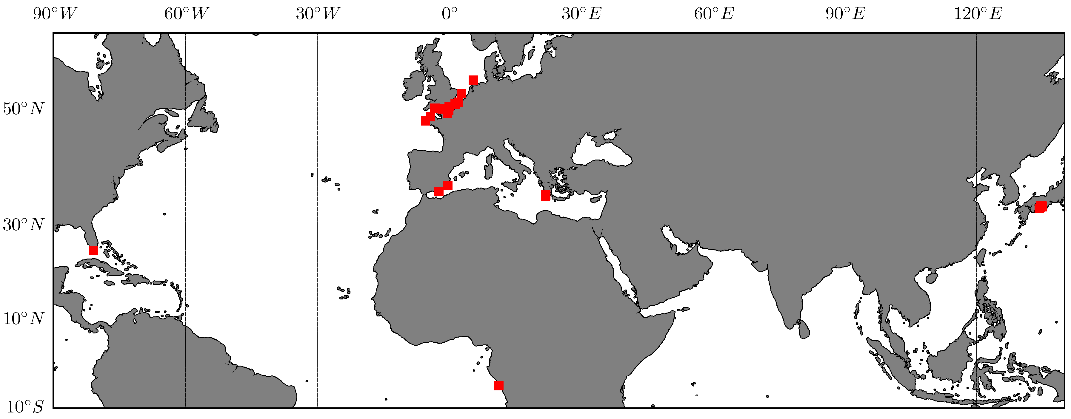
Specific platforms have been selected to test the extrapolation capabilities of the network. In this case, complete platform datasets have been isolated and used as test sections of the dataset. Figure 9 shows the selected locations of the used buoys, in this case platforms in the Mediterranean Sea, English Channel, Florida, Japan and Congo have been selected. The same platforms have been used for both temperature and salinity extrapolation.

Figure 10 shows the training and test correlation and residuals, as well as matching between ground truth and estimated temperature. Residuals are consistent with the interpolation counterpart, showing a most common error of about 0.4 ${}^{°}$C, while the MAE is lower in the extrapolation case. This is highly influenced by the smaller number of points tested compared to the size of the training dataset, as less outliers are obtained. The central panel shows how the network is able to simulate the trends in data points accurately.

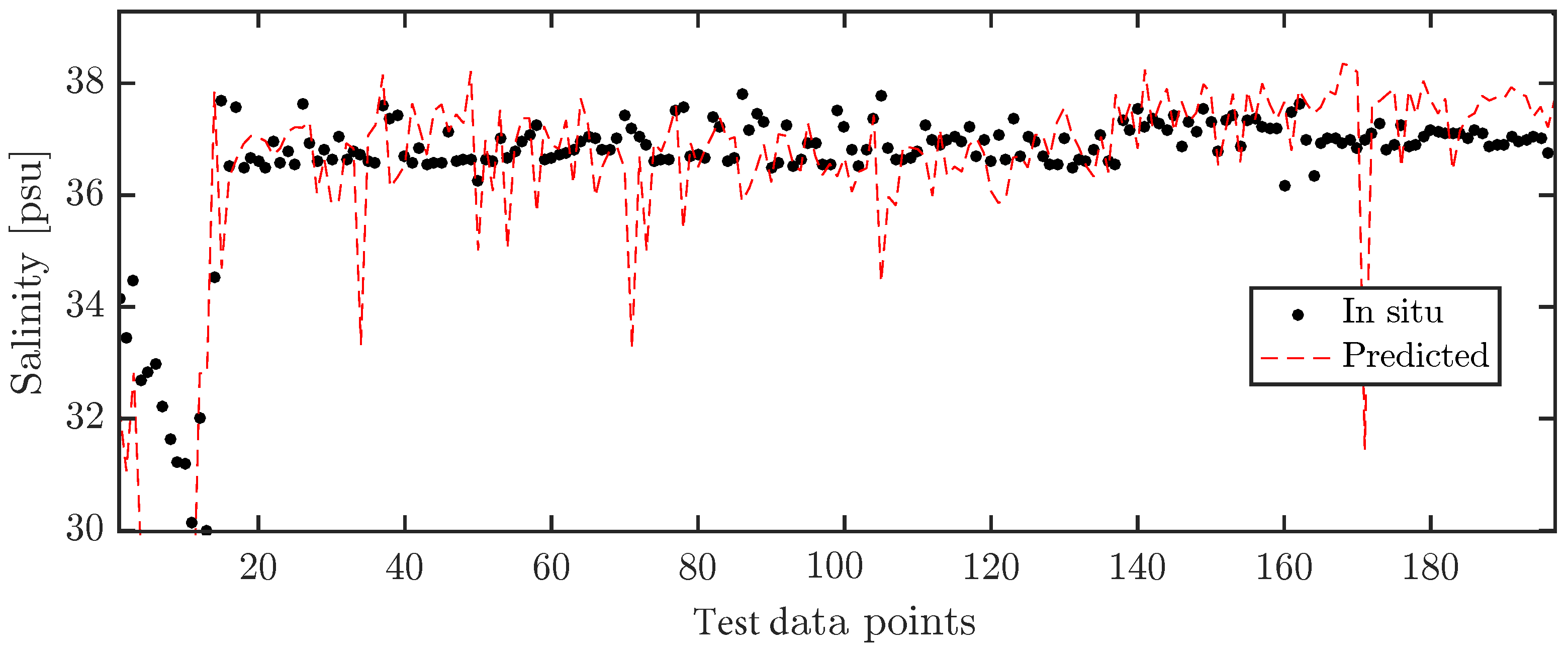
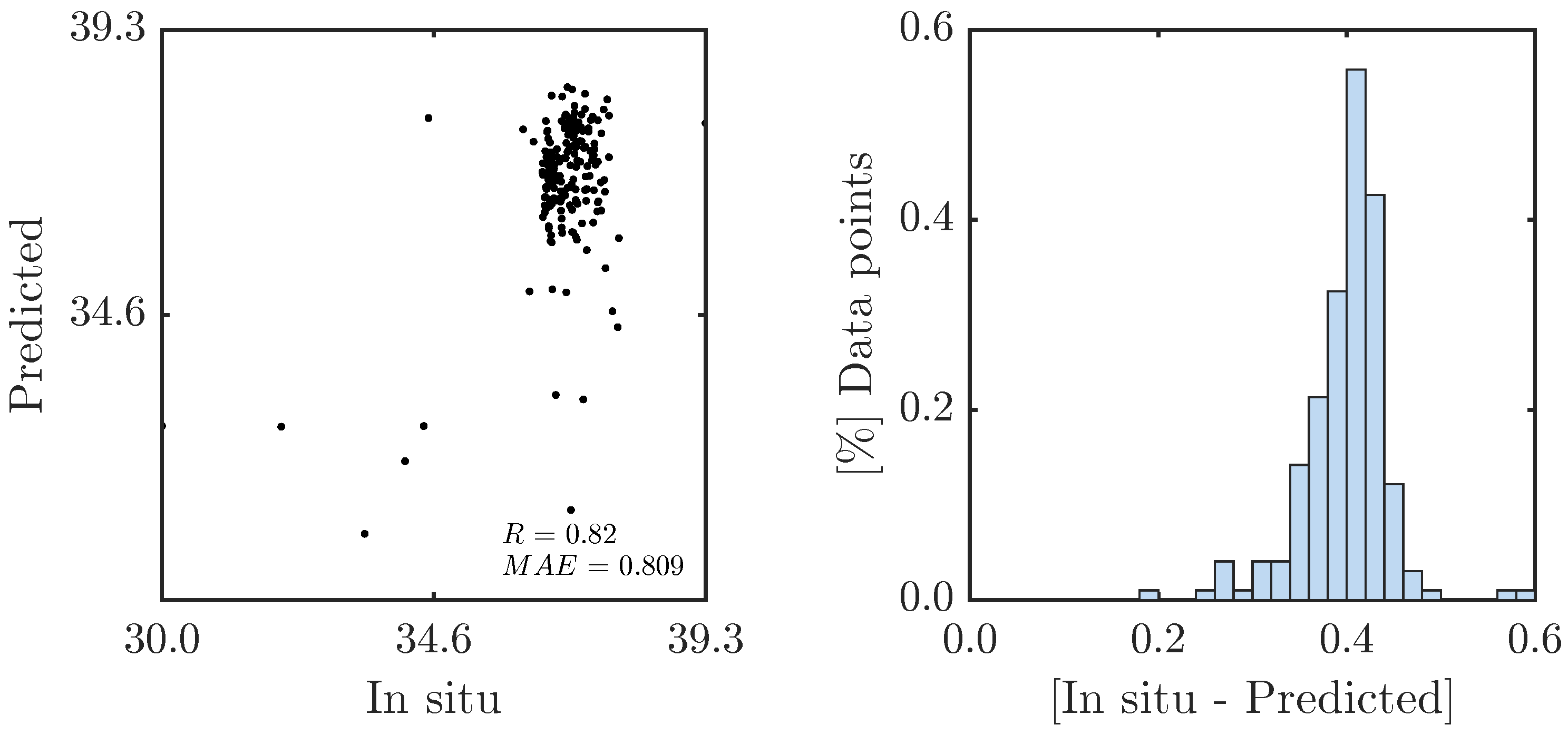
3.5. Salinity Extrapolation

Results in Figure 11 show residuals slightly asymmetrical centred in 0.4 PSU, while the MAE is about 0.8 PSU, considerably lower than the interpolation result. The correlation is strong, although most of the points are placed in a very narrow range in between 36 and 38 PSU. However, during training we had salinity values ranging from 0 PSU to 42 PSU consistently, as showed in Figure 6. Extrapolation results show a similar pattern to that presented in interpolation in the range given, which is reassuring of the consistent prediction behaviour of the neural network. Peaks are observed in the comparison showed in the central panel. This might have been caused by the inclusion of the firsts section of the dataset, where lower values of salinity are present.

3.6. Evaluation: Mapping Sea Surface Salinity and Temperature at the Guadalquivir River Mouth and the Bay of CáDiz

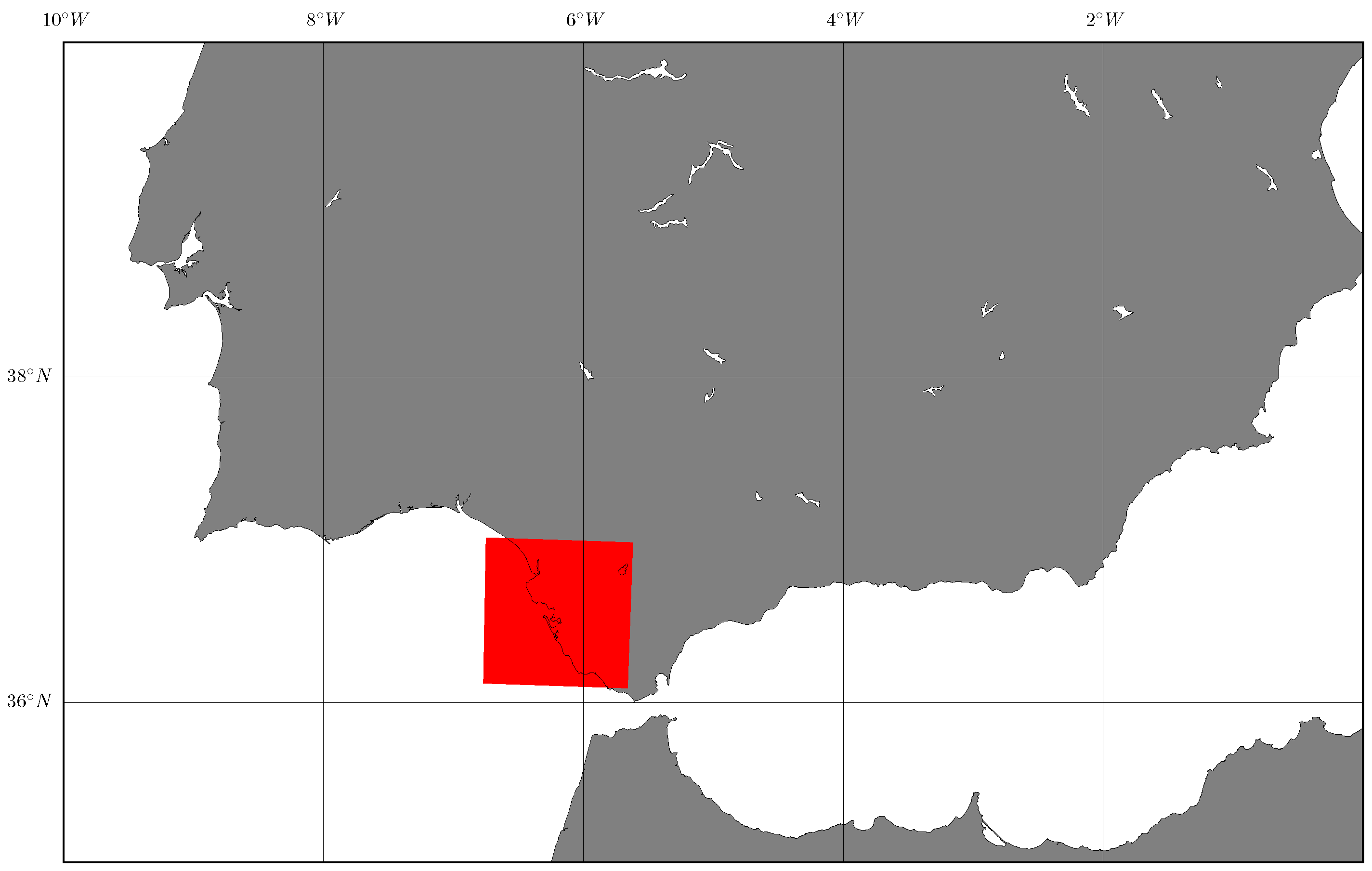
In this section, the evaluation of the trained neural network over a complete Sentinel-2 tile is presented. Tiles from the area around the Guadalquivir River mouth and Bay of Cádiz (South–West Spanish coast) have been downloaded with pixel resolution of 100 m $\times 100$ m during 2016 (tile 29SQA), see Figure 12. This area has been selected for its multiple interesting features: the Guadalquivir River mouth provides a good overview of mixing processes (fresh-sea water); on the other hand, the combination of high temperatures and low river discharge during summer with the relatively cold temperature of the Atlantic Ocean is useful to observe the behaviour of the network.

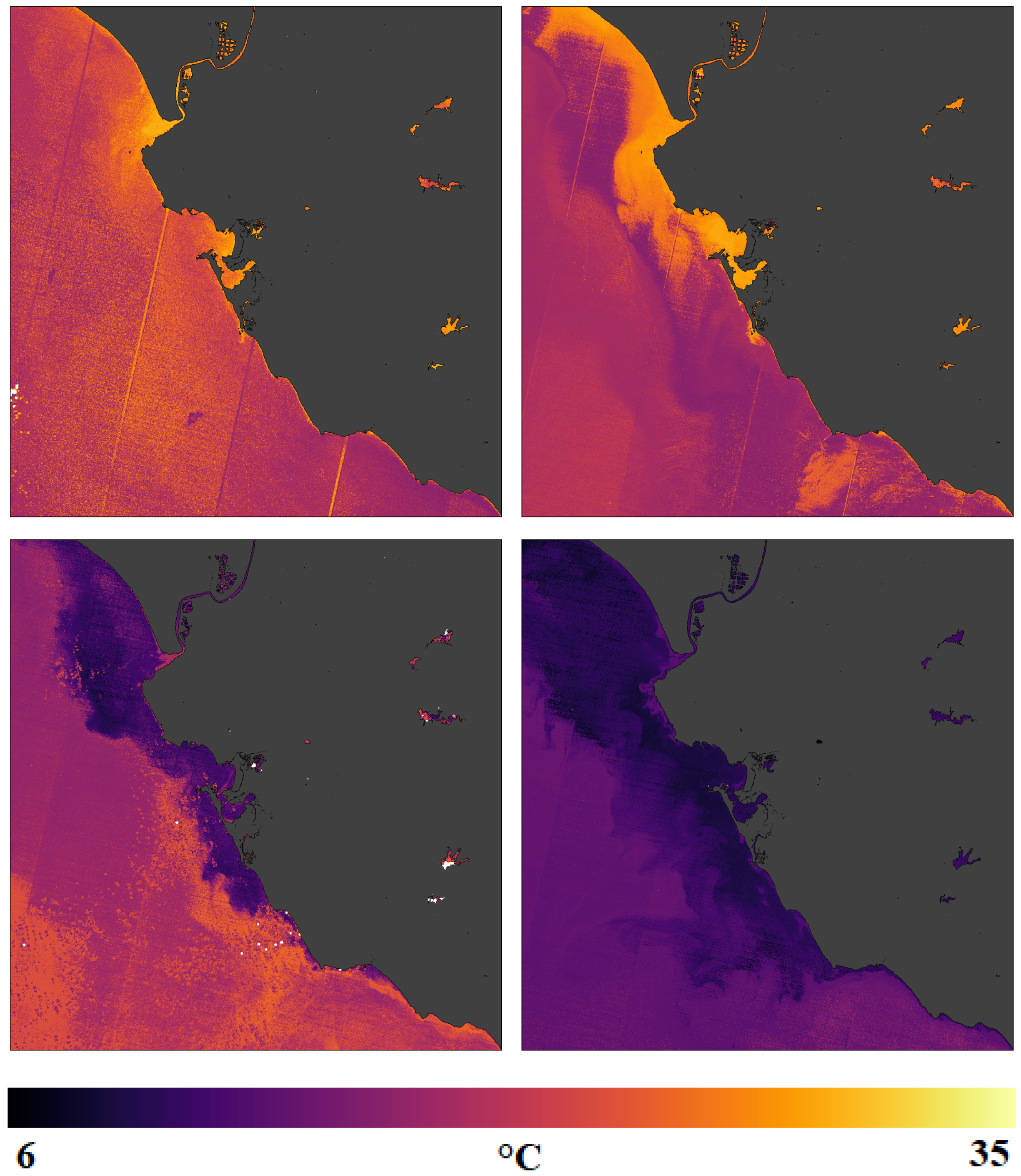
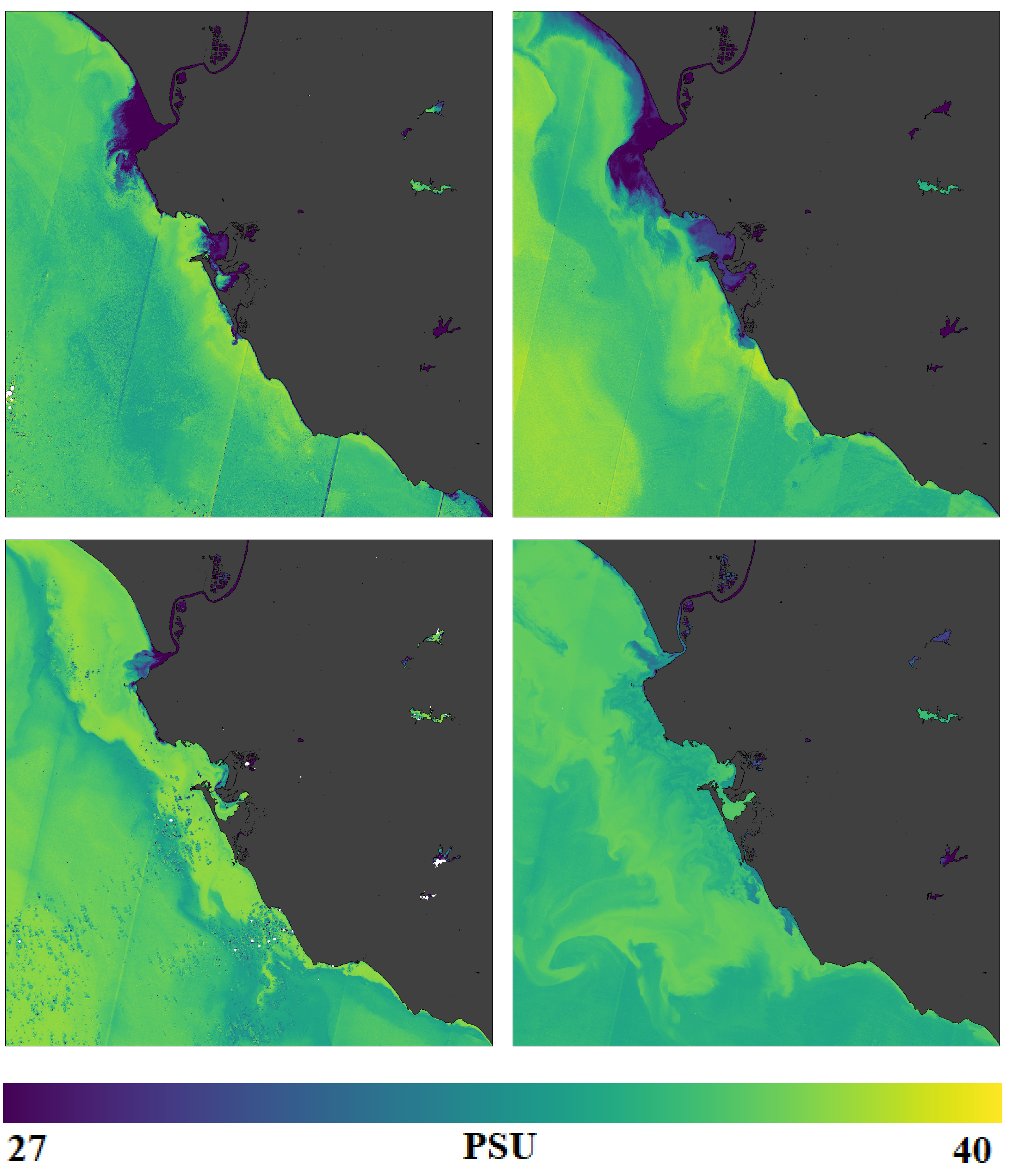
Although outliers have been observed in both interpolation and extrapolation problems, we expect to observe the more general behaviour of the river–ocean interaction and other features in this evaluation. Figure 13 and Figure 14 present temperature and salinity results on the selected area during 2016. Representative images of the four seasons are plotted (May, August, October and December). Slight clouds have been painted in white for better contrast.

During spring and summer, the river discharge is lower and the water is warmer than the ocean water. Clear discharge patterns are observed during these months in Figure 13. In contrast, those same months in Figure 14 show stronger stratification—the river plume of fresh water is clearly observed, presenting characteristic eddies at the boundary. In contrasts, the autumn and winter months show lower temperatures, and less obvious temperature mixing processes. A characteristic band of colder temperatures is placed nearly parallel to the coastline. The bathymetry in the area is also parallel to the coast, being nearly flat in the first kilometres. The observed phenomenon can be caused by a current forced by the sea floor. In terms of salinity during colder months, mixing processes and vortices are still observed. A particular situation is observed in the last figure (December), where the intrusion of sea water can be clearly observed into the river mouth. Following the historical tide records in [32] from the Bonanza Tide Gauge (which is placed at the river mouth), the tide that day (23 December 2016) at the time the Sentinel-2 image was taken (11:14 a.m.) is about 2 m (tide just reached high-tide), being consistent with the observed behaviour.

An undesired effect that is observed in some of the images is the appearance of sun glitter inherited from the original Sentinel-2 images. Following the Sentinel-2 Data Quality Report, [33], surface reflectance effects are present due to the variation on viewing angles for even and odd detectors in the satellite. A difference in measured radiometry can be observed on sea surfaces, represented by a subtle stripe pattern due to this parallax effect. However, although the transition between stripes is observed in the results from the neural network, the general behaviour is maintained in the transition. Although sun–glint can be corrected using the SWIR information, the authors decided to show the raw results of the methodology to be consistent with the line of the paper. We intend to include this in future analyses.

Moreover, an unexpected behaviour was that the neural network was able to estimate salinity and temperature in the reservoirs and lakes in land. As the network has not been trained with data from reservoirs, results in this case are not valid, but it would be interesting to validate these observations with water quality measurements in those areas.

4. Conclusions

This paper presents a methodology to obtain high-resolution values of sea surface salinity and temperature in the global ocean by using satellite data without any band data pre-processing or atmospheric corrections. Sentinel-2 Level 1-C Top of Atmosphere reflectance data has been used here. A deep neural network has been built to link band information with in situ data from different buoys, vessels, drifters, and other platforms around the world. This in situ information has been obtained from the Copernicus Marine In Situ platform.

The neural network presented in this paper outperformed classical architectures tested for regression problems. The Sentinel-2 data was processed using Google Earth Engine in areas of 100 m $\times 100$ m around relevant platforms. Accurate salinity values are estimated for the first time without using temperature as input in the network. Salinity results depend only on direct satellite observations. However, a clear dependency on temperature ranges is observed, with less accurate estimations for location where ocean temperature falls below 10 ${}^{°}$C. The reasons for this is unclear from the findings presented in this paper, but could be linked to the amount of available data in areas with lower temperatures and the ability of the network to predict them, or the presence of other physical phenomena such as freezing and mixing. In order to overcome this issue more information is needed in higher latitudes and areas where other phenomena, such as mixing processes and freezing, are representative. Extended information would also help reducing the amount of uncertainties on outliers in prediction.

The neural network has good interpolation and extrapolation capabilities. Mean absolute errors of 0.8 PSU and 1.3 ${}^{°}$C with correlation coefficients of $82\%$ and $84\%$ for salinity and temperature, respectively, are obtained in test locations. The most common error for both temperature and salinity is 0.4 ${}^{°}$C and 0.4 PSU. A sensitivity analysis was also performed, showing that outliers are present in areas where the number of observations is lower. The network is tested in a complete tile over the Guadalquivir River mouth, in the south-west coast of Spain. Results show clear seasonal patters, as well as a sensible interaction between river discharge and ocean intrusions that matches records from local buoys. Issues with sun glitter are observed in some images, although the general behaviour remains. This issue could be sorted by using SWIR information to identify sun glitter in each image. This methodology is relevant for detailed coastal and oceanographic applications. The time for data pre-processing is reduced significantly compared with previous approaches. Moreover, the methodology is applicable to a wide range of satellites, as the information is directly obtained from Top of Atmosphere information.

References

- Sang, Y.; Karayaka, H.B.; Yan, Y.; Yilmaz, N.; Souders, D. Ocean (Marine) Energy. Compr. Energy Syst. 2018, 1, 733–769. [Google Scholar]
- National Oceanic and Atmospheric Administration, U.S. Department of Commerce. Why do Scientists Measure Sea Surface Temperature? 2018. Available online: https://oceanservice.noaa.gov/facts/sea-surface-temperature.html (accessed on 1 June 2019).
- Chen, S.; Hu, C. Estimating sea surface salinity in the northern Gulf of Mexico from satellite ocean colour measurements. Remote Sens. Environ. 2007, 201, 115–132. [Google Scholar] [CrossRef]
- European Commission. Copernicus Marine Environment Monitoring Service. 2018. Available online: http://marine.copernicus.eu/ (accessed on 1 June 2019).
- Barre, H.M.J.P.; Duesmann, B.; Kerr, Y.H. SMOS: The Mission and the System. IEEE Trans. Geosci. Remote Sens. 2008, 46, 587–593. Available online: https://www.esa.int/Our_Activities/Observing_the_Earth/SMOS (accessed on 1 June 2019). [CrossRef]
- Le Vine, D.M.; Lagerloef, G.S.E.; Ral Colomb, F.; Yueh, S.H.; Pellerano, F.A. Aquarius: An Instrument to Monitor Sea Surface Salinity From Space. IEEE Trans. Geosci. Remote Sens. 2007, 45, 2040–2050. Available online: https://www.nasa.gov/mission_pages/aquarius/overview (accessed on 1 June 2019). [CrossRef]
- Parkinson, C.L. Aqua: An Earth-Observing Satellite mission to examine water and other climate variables. IEEE Trans. Geosci. Remote Sens. 2003, 41, 173–183. Available online: https://oceancolor.gsfc.nasa.gov/data/aqua/ (accessed on 1 June 2019). [CrossRef]
- Gregg, W.W.; Patt, F.S.; Woodward, R.H. Development of a Simulated Data Set for the SeaWiFS Mission. IEEE Trans. Geosci. Remote Sens. 1997, 35, 421–435. Available online: https://oceancolor.gsfc.nasa.gov/SeaWiFS (accessed on 1 June 2019). [CrossRef]
- Pichel, W.; Sapper, J.; Duda, C.; Maturi, E.; Jarva, K.; Stroup, J. CoastWatch Operational Mapped AVHRR Imagery. In Proceedings of the IGARSS ’94—1994 IEEE International Geoscience and Remote Sensing Symposium, Pasadena, CA, USA, 8–12 August 1994; Volume 2, pp. 1219–1221. Available online: https://coastwatch.noaa.gov (accessed on 1 June 2019).
- Shibata, A.; Imaoka, K.; Kachi, M.; Fujimoto, Y.; Mutoh, T. AMSR/AMSR-E Sea Surface Temperature Algorithm Development. In Proceedings of the IGARSS 2003—IEEE International Geoscience and Remote Sensing Symposium, Toulouse, France, 21–25 July 2003. [Google Scholar] [CrossRef]
- Gentemann, C.L.; Meissner, T.; Wentz, F.J. Accuracy of satellite sea surface temperatures at 7 and 11 GHz. IEEE Trans. Geosci. Remote Sens. 2010, 48, 1009–1018. [Google Scholar] [CrossRef]
- Aparna, S.G.; D’Souza, S.; Arjun, N.B. Prediction of daily sea surface temperature using Artificial Neural Networks. Int. J. Remote Sens. Remote Sens. Lett. 2018, 39, 4214–4231. [Google Scholar] [CrossRef]
- Garcia-Gorriz, E.; Garcia-Sanchez, J. Prediction of sea surface temperatures in the western Mediterranean Sea by neural networks using satellite observations. Geophys. Res. Lett. 2007, 34. [Google Scholar] [CrossRef]
- Patil, K.; Deo, M.C. Prediction of sea surface temperatures by combining numerical and neural techniques. J. Atmos. Ocean. Technol. 2016, 33, 1715–1726. [Google Scholar] [CrossRef]
- Brewin, R.J.W.; Mora, L.; Billson, O.; Jackson, T.; Russell, P.; Brewin, T.G.; Shutler, J.D.; Miller, P.I.; Taylor, B.H.; Smyth, T.J.; et al. Evaluating operational AVHRR sea surface temperature data at the coastline using surfers. Estuarine Coast. Shelf Sci. 2017, 196, 276–289. [Google Scholar] [CrossRef]
- Marghany, M.; Hashim, M.; Cracknell, A.P. Modelling Sea Surface Salinity from MODIS Satellite Data. In Proceedings of the International Conference on Computational Science and its Applications, Fukuoka, Japan, 23–26 March 2010; pp. 545–556. [Google Scholar]
- Geiger, E.F.; Grossi, M.D.; Trembanis, A.C.; Kohut, J.T.; Oliver, M.J. Satellite–derived coastal ocean and estuarine salinity in the Mid–Atlantic. Cont. Shelf Res. 2013, 63, S235–S242. [Google Scholar] [CrossRef]
- Olmedo, E.; Taupier–Letage, I.; Turiel, A.; Alvera-Azcárate, A. Improving SMOS Sea Surface Salinity in the Western Mediterranean Sea through Multivariate and Multifractal Analysis. Remote Sens. 2018, 10, 485. [Google Scholar] [CrossRef]
- Srokosz, M.; Banks, C. Salinity from space. Weather 2019, 74, 21–40. [Google Scholar] [CrossRef]
- Mavrocordatos, C.; Berrutti, B.; Aguirre, M.; Drinkwater, M. The Sentinel-3 Mission and its Topography Element. In Proceedings of the 2007 IEEE International Geoscience and Remote Sensing Symposium, Barcelona, Spain, 23–28 July 2007; pp. 3529–3532. Available online: https://earth.esa.int/web/guest/missions/esa-eo-missions/sentinel-3 (accessed on 1 June 2019).
- European Commission. Insitu Near Real Time Observations. 2018. Available online: http://marine.copernicus.eu/services-portfolio/access-to-products/?option=com_csw&view=details&product_id=INSITU_GLO_CARBON_NRT_OBSERVATIONS_013_049 (accessed on 1 June 2019).
- European Commission. Insitu Reprocessed Observations. 2018. Available online: http://marine.copernicus.eu/services-portfolio/access-to-products/?option=com_csw&view=details&product_id=INSITU_GLO_TS_REP_OBSERVATIONS_013_001_b (accessed on 1 June 2019).
- Martimort, P.; Arino, O.; Berger, M.; Biasutti, R.; Carnicero, B.; Del Bello, U.; Fernandez, V.; Gascon, F.; Greco, B.; Silvestrin, P.; et al. Sentinel-2 Optical High Resolution Mission for GMES Operational Services. In Proceedings of the 2007 IEEE International Geoscience and Remote Sensing Symposium, Barcelona, Spain, 23–27 July 2007; pp. 2677–2680. Available online: https://sentinel.esa.int/web/sentinel/missions/sentinel-2 (accessed on 1 June 2019).
- Google. Google Earth Engine. 2018. Available online: https://code.earthengine.google.com (accessed on 1 June 2019).
- Gorelick, N.; Hancher, M.; Dixon, M.; Ilyushchenko, S.; Thau, D.; Moore, R. Google Earth Engine: Planetary-scale geospatial analysis for everyone. Remote Sens. Environ. 2017, 202, 18–27. [Google Scholar] [CrossRef]
- Nielsen, M.A. Neural Networks and Deep Learning. Determination Press, 2015. Available online: http://neuralnetworksanddeeplearning.com (accessed on 1 June 2019).
- Kastner, F.; Jansen, B.; Kautz, F.; Hubner, M. Exploring Deep Neural Networks for Regression Analysis. In Proceedings of the Eighth International Conference on Performance, Safety and Robustness in Complex Systems and Applications, Tsukuba, Japan, 22–26 April 2018. [Google Scholar]
- Ioffe, S.; Szegedy, C. Batch Normalization: Accelerating Deep Network Training by Reducing Internal Covariate Shift. arXiv 2015, arXiv:1502.03167. [Google Scholar]
- Schmidhuber, J. Deep learning in neural networks: An overview. Neural Networks 2015, 61, 85–117. [Google Scholar] [CrossRef] [PubMed] [Green Version]
- Veit, A.; Wilber, M.; Belongie, S. Residual Networks Behave Like Ensembles of Relatively Shallow Networks. arXiv 2016, arXiv:1605.06431. [Google Scholar]
- Srivastava, R.K.; Greff, K.; Schmidhuber, J. Highway Networks. arXiv 2015, arXiv:1505.00387. [Google Scholar]
- De España, G.; del Estado, P. Available online: https://portus.puertos.es/ (accessed on 1 June 2019).
- European Space Agency. Available online: https://sentinel.esa.int/documents/247904/685211/Sentinel-2_L1C_Data_Quality_Report (accessed on 1 June 2019).
Figure 1.
Map of the available platforms since 2015 containing salinity and temperature data (approx. 4600 valid platforms.
Figure 2.
Map of the Western Mediterranean Sea showing an example subset with location of observations from moorings (black squares), and vessels (red dots).
Figure 3.
Schematic of the structures of neural networks used in the paper with temperature as example output. Deep Neural Network (left) and Deep Neural Network with shortcuts (right). The sketches represents networks with n layers fully connected; the input neurons are the variables summarised in Table 4 and Table 5— note that band QA60 has not been used as input for the Neural Network.
Figure 4.
Temperature interpolation. Training: predicted vs. in situ data (top left); histogram of residuals in training (top right). Test: predicted vs. in situ data (centre left); histogram of residuals (centre right); difference between measured and predicted temperature in test locations (bottom). Units of temperature are C.
Figure 5.
Detail extracted from Figure 4 showing the difference between measured and predicted temperature in test locations for the United States (left) and Europe (right).
Figure 6.
Salinity interpolation. Training: predicted vs. in situ data (top left); histogram of residuals in training (top right). Test: predicted vs. in situ data (centre left); histogram of residuals (centre right); difference between measured and predicted salinity in test locations (bottom). Units of salinity are PSU.
Figure 7.
Detail extracted from Figure 6 showing the difference between measured and predicted salinity in test locations for the United States (left) and Europe (right).
Figure 8.
Histogram of number of observations and errors () for salinity (top panels) and temperature (bottom panels). Left panels show latitude and right panels longitude.
Figure 9.
Map of buoys used for salinity and temperature extrapolation.
Figure 10.
Temperature extrapolation. Test: predicted and in situ data time series (top); predicted vs. in situ data (bottom left); histogram of residuals (bottom right). Units of temperature are C.
Figure 11.
Figure 12.
Location of evaluation area near Cádiz (South-West Spain).
Figure 13.
Evaluation of neural network: temperature prediction at the mouth of the Guadalquivir River during 2016 in May (top left), August (top right), October (bottom left) and December (bottom right). Units of temperature are C.
Figure 14.
Evaluation of neural network: salinity prediction at the mouth of the Guadalquivir River during 2016 in May (top left), August (top right), October (bottom left) and December (bottom right). Units of salinity are PSU.