Article

Spatial–Spectral Fusion in Different Swath Widths by a Recurrent Expanding Residual Convolutional Neural Network

1
School of Geodesy and Geomatics, Wuhan University, Wuhan 430079, China
2
School of Resource and Environmental Sciences, Wuhan University, Wuhan 430079, China
*
Author to whom correspondence should be addressed.
Remote Sens. 2019, 11(19), 2203; https://0-doi-org.brum.beds.ac.uk/10.3390/rs11192203
Submission received: 18 July 2019 / Revised: 5 September 2019 / Accepted: 12 September 2019 / Published: 20 September 2019
(This article belongs to the Special Issue Remote Sensing Image Restoration and Reconstruction)

Abstract

:
The quality of remotely sensed images is usually determined by their spatial resolution, spectral resolution, and coverage. However, due to limitations in the sensor hardware, the spectral resolution, spatial resolution, and swath width of the coverage are mutually constrained. Remote sensing image fusion aims at overcoming the different constraints of remote sensing images, to achieve the purpose of combining the useful information in the different images. However, the traditional spatial–spectral fusion approach is to use data in the same swath width that covers the same area and only considers the mutually constrained conditions between the spectral resolution and spatial resolution. To simultaneously solve the image fusion problems of the swath width, spatial resolution, and spectral resolution, this paper introduces a method with multi-scale feature extraction and residual learning with recurrent expanding. To discuss the sensitivity of convolution operation to different variables of images in different swath widths, we set the sensitivity experiments in the coverage ratio and offset position. We also performed the simulation and real experiments to verify the effectiveness of the proposed framework with the Sentinel-2 data, which simulated the different widths.

Graphical Abstract

1. Introduction

With the rapid development of remote sensing technology, a pattern of joint multi-spatio-spectral Earth observation has been formed under different surface coverages and revisit cycles. However, due to the difference in the instrument design, platform height, data storage, and transmission, the spatial resolution, spectral resolution, and swath width of the images restrict each other. Generally speaking, due to the limited amount of incident energy, a satellite system can usually only provide data with either a high spatial resolution but a small number of spectral bands, or with a large number of spectral bands but a reduced spatial resolution [1]. Specifically, those bands in the multi-channel images obtained by sensors such as the Moderate Resolution Imaging Spectroradiometer (MODIS) and Sentinel-2 sensors have different spatial resolutions. In addition, there is also a critical tradeoff between the swath width and the other sensor properties, including the spatial resolution and spectral resolution. To acquire wider-swath-width images, the Landsat Thematic Mapper (TM) sensor reduces the 30 m spatial resolution to 120 m. As for the SPOT and Gaofen-1 (GF-1) satellites, acquiring high spatial resolution images suffers from a small swath width of 60 km compared to the swath width of 800 km in its wide-swath-width imaging mode. These limitations of the sensor properties mean that it is difficult for us to simultaneously observe the ground surface at both a fine resolution and a broad scale. Therefore, many researchers have developed fusion methods to improve these properties of the original images, to promote the performance of remote sensing applications.
Image fusion technology, which is an important means of information integration in remote sensing, is often used to solve the problems caused by spatial and spectral limitations. By taking advantage of the complementary information of two images with different spatial resolutions and spectral resolutions, high spatial resolution (HR) images with a high spectral resolution can be synthesized [2,3]. The typical approach is spatial–spectral fusion, which has attracted extensive research, including component substitution methods [2,3,4,5], multi-resolution analysis methods [6,7,8,9,10], and model optimization based methods [11,12,13,14,15,16,17]. For example, researchers have used robust principal component analysis (PCA) to decompose multispectral images, and have used panchromatic images to incorporate spatial information into multispectral images [2]. Other researchers have introduced wavelet transform to decompose both the multispectral images and the panchromatic images and have then fused the different components based on certain rules, such as the weighted averaging method, finally reconstructing HR multispectral images [7]. In addition, Song et al. [18] proposed an image degradation model from SPOT5 to TM to improve the spatial resolution of the TM multispectral bands by dictionary learning.
At present, deep learning is being gradually introduced to solve the spatial–spectral fusion problem [19,20,21,22]. In these methods, a neural network is trained to extract the spatial and spectral features and then fuse them to obtain high spatial resolution and high spectral resolution (HRHS) images. However, for these spatial–spectral fusion methods, the low spatial resolution (LR) image can only be well sharpened when the images cover the same area and the same spectral range.
With the development of remote sensing satellites and the diversity of sensor imaging modes, there are two main challenges. Firstly, the different-band images in one multi-channel image have different spatial resolutions and non-overlapping spectral regions [23]. The traditional spatial and spectral fusion method, which is limited to the same spectral range, has difficulty dealing with this problem. When the spectral range of the high and low-resolution images is not the same, injecting spatial information from an HR band into the low-resolution band is prone to spectral distortion, which makes it difficult to maintain the spectral information of the images. To deal with the above fusion problem, multi-band fusion has recently been proposed [24]. For example, Wang et al. [25,26] proposed a two-stage fusion method based on geostatistics, which first creates a single HR image from the available high spatial resolution images and then use area-to-point kriging to upscale the residuals, so as to improve the spatial resolution. However, these methods based on geostatistics cannot be easily extended to images produced by other sensors. Inspired by deep learning, Palsson et al. [23] proposed to fuse the Sentinel-2 images using a deep residual network. However, the existing methods cannot accurately express the response functions between different spectra when the image’s spatial resolution is enhanced, which causes spectral distortion.
Secondly, the different-band images in different imaging modes have different spatial resolutions and swath widths [27]. Thus, a part of the image needs to be clipped because of the inconsistency of the image swath width and size, which leads to a waste of information. Faced with the fusion of images with different swath widths, the simple way is to interpolate the non-overlapping region, and then splice the fusion result with the overlapping region. However, with the under-utilization of the complementary information in the overlapping regions, the fused image suffers from insufficient high-frequency information and smoothed texture and edge regions. To address this issue, Song et al. [18] obtained a satisfactory wide spatial detail enhancement result by establishing a coupled sparse model of the overlapping region. In addition, Sun et al. [28] realized the effective fusion of EO-1 Hyperion hyperspectral and Advanced Land Imaging (ALI) wide-swath-width multispectral images of the same spatial resolution by establishing a response relation model between the spectra. However, the spatial resolution and spectral resolution cannot be simultaneously enhanced.
The spectral, spatial, and swath-width enhancement of remote sensing images has been considered in many studies. However, the above methods cannot simultaneously incorporate the spectral, spatial, and swath-width information into one model. To directly produce HRHS images with a wide swath width, sufficient spatial and spectral information should be extracted from the images, which can be viewed as a nonlinear mapping. Deep learning is a way of exploring the nonlinear mapping between data, which can easily fit an extremely complex nonlinear relationship through a nonlinear activation function. Because of this advantage, many scholars have applied deep learning to image fusion and super-resolution tasks. Among the well-known convolutional neural networks (CNNs) are the super-resolution convolutional neural network (SRCNN) [29], the pansharpening by convolutional neural network (PCNN) [20], the very deep convolutional network (VDSR) [30], ResNet [23], VDsen2 [31], and the deep residual pansharpening neural network (DRPNN) [22].
In this paper, we propose a deep convolutional neural network with a residual learning (DRCNN) based width-space-spectrum (WSS) fusion method to obtain HR multispectral images with both a high spectral resolution and wide swath width. By mining the nonlinear relationship between the HR and LR information in the overlapping areas and mapping the transformation of the different spectral information, an integrated framework is built for WSS fusion. The main contributions of this paper include:
(1) A spatial–spectral joint learning algorithm for different-swath-width images based on a deep residual CNN is proposed. The deep learning algorithm provides more reliable prior spatial and spectral knowledge for the non-overlapping region, modeling by training the mapping between the spatial and spectral information in the overlapping area.
(2) By exploring the sensitivity of the CNN to different-swath-width image coverage ratios and offsets, a recurrent expanding reconstruction strategy is established. Through the discussion of the effects of different variables on the network performance, a highly applicable reconstruction strategy is put forward.
The rest of this paper is structured as follows. In Section 2, the overall framework of the proposed method and the recurrent expanding reconstruction strategy are introduced. In Section 3, the experiments and the results are discussed. Finally, in Section 4, a summary is given.

2. Methodology

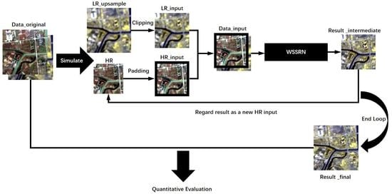
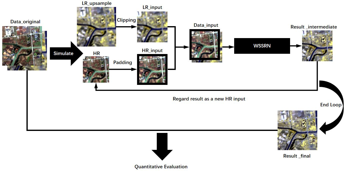
2.1. Width-Space-Spectrum Fusion

During the imaging process for remote sensing satellites, the sensor systems have an inevitable impact on the spatial degradation, the spectral resolution, and the swath width. Different sensors generate different resolution properties. To describe the relationships between the different observed images, the specific observation model is defined as follows:
Y = S A n g l e _ Y ( A M X ) + N Y
Z = S A n g l e _ Z ( B N X ) + N Z
where X represents the original HRHS image with a wide swath width; Y represents the high spatial resolution and low spectral resolution (HRLS) image with a narrow swath width; Z represents the low spatial resolution and high spectral resolution (LRHS) image with a wide swath width; A and B represent the spectral response transform factors of the different imaging modes; M and N represent the corresponding spatial degradation factors; S is the field of view in different imaging modes, which can be treated as a mask; A n g l e _ Y is the view angle in the HR imaging mode; A n g l e _ Z is the view angle in wide-swath-width imaging mode; and N Y and N Z represent the additive noise present in the real multispectral image.
The WSS fusion problem is to reconstruct the approximate HR image X ^ with high spectral resolution and wide swath width using the LR image Z with a wide swath width and the HR image Y with a narrow swath width. For this fusion, due to the missing information caused by the different swath widths, the fusion result cannot be directly obtained by a simple linear method. The key to achieving WSS fusion is to learn the relationship between the narrow-swath-width HR image and the wide-swath-width LR image, which can be expressed as the following nonlinear problem:
X ^ = f ( Y , Z ; θ )
where f ( · ; θ ) is the nonlinear model, which can be trained in the deep learning approach proposed in this paper, and θ is the parameter in the DRCNN, which represents the weights and biases in different convolution kernels and the hyper-parameters in the network. The key to WSS fusion is to design a better network structure and solve the parameters, which can be expressed as:
θ = arg min θ X f ( Y , Z ; θ ) 2 2 + α Ω ( θ )
where α is a tradeoff parameter and Ω ( · ) is a regularization term that prevents overfitting. In this paper, the weight decay term Ω ( θ ) = 1 2 θ 2 2 is introduced as a regularized penalty function.
From Equation (4), it can be concluded that the solution to the WSS fusion problem lies in the design of a framework suitable for the fusion problem and conducive to optimization. The network framework proposed in this paper is elaborated in Section 2.2.

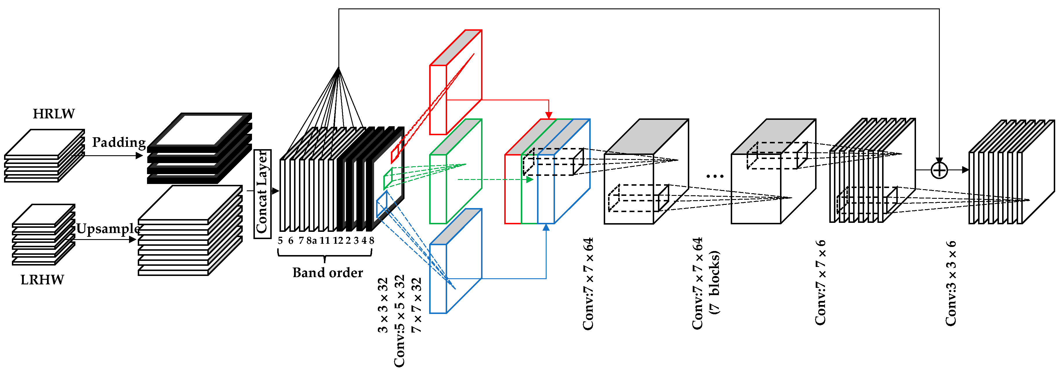
2.2. Network Framework

As shown in Figure 1, the framework of the network proposed in this paper is to undertake WSS fusion by constantly expanding the image recursively. Based on the residual network, a width-space-spectrum residual network (WSSRN) model is proposed to extract the spatial features and spectral features with different resolutions and swath widths. This network expands the image by a few pixels at every iteration. It is worth noting that the weights of the network are shared between each iteration, which is good for network training. To fuse the HR and LR images with different swath widths, take Sentinel-2 for example. The LR image is first upsampled, and the HR image is then expanded to the same size as the upsampled LR image. The input images are then concatenated in turn, as shown in Figure 1, which allows images with the same resolution to be closer to better extract features. After feeding the images into the network, the multi-scale convolutional layers are used to extract the features from the images with different swath widths, which consists of three convolution layers with sizes of 3 × 3 × 32, 5 × 5 × 32, and 7 × 7 × 32. To ensure the network can be easily optimized, a skip connection between the input LR image and the residual image is used. There are six convolution blocks between the skip connection and multi-scale convolutional layers, which are composed of a 7 × 7 × 64 convolution layer followed by a Rectified Linear Unit (ReLU). After training such a network, the fused image can be continuously updated through a recurrent expanding strategy to finally obtain the HR and wide-swath-width multispectral image.

2.3. The Residual Convolutional Neural Network

In this paper, the CNN differs from an ordinary neural network in that the pooling layer is removed, which causes the loss of HR information. The purpose of the convolution operation is to extract different features from the image. After the input image is convoluted by the convolution kernel, the feature map can be excavated by the non-linearization of an activation function, which is defined as follows:
F l j = g ( W l j F l 1 + b l j )
where F l j represents the j -th feature map of the l th layer, F l 1 indicates the set of input feature maps corresponding to the j -th feature map, W l j indicates the weights of the convolution kernel between the feature maps of the l 1 -th layer and the j -th feature map of the l -th layer, and b l j represents the bias of the j -th feature map of the l -th layer. Here, g means the rectified linear unit (ReLU), which is selected as the activation function. Its specific function expression is:
g ( x ) = max ( x , 0 )
After the convolutional layer and the activation function complete the feature extraction, the extracted features are further input into the reconstruction output layer, and the reconstruction output layer works as “fusion reconstruction” in the entire CNN, which is essentially a convolutional layer. Passing through the previous feature extraction work, the spectral features and the spatial features are distributed in different channels, so it is necessary that a convolutional layer is used to fuse the features.
For a traditional CNN, the deeper the network, the more parameters it has and the more powerful nonlinear presentation capabilities it obtains. However, as the network gets deeper and deeper, it will cause the gradient disappearance during the training process, which leads to the weights of the previous convolutional layers being unoptimized [32].
To solve this problem, this paper draws on the idea of a deep residual network. However, in this paper, the structure of the residual block in a deep residual network is not directly used, because such a structure makes the network too complicated. Only a single head-to-tail skip connection is used to increase the gradient in the network back-propagation. The loss function of the network is as follows:
L o s s ( θ ) i = i = 0 n ( X i Z i ) ( f ( Y , Z ; θ ) i Z i ) 2 2
where X i represents the i -th band of the ground truth, and n represents the number of the band. This connection can be called a “global skip connection”, which avoids the problem of the vanishing gradient in the network back-propagation. Furthermore, this skip connection also accelerates the convergence of the network, because, when the gradient is larger, the parameter optimization is faster.

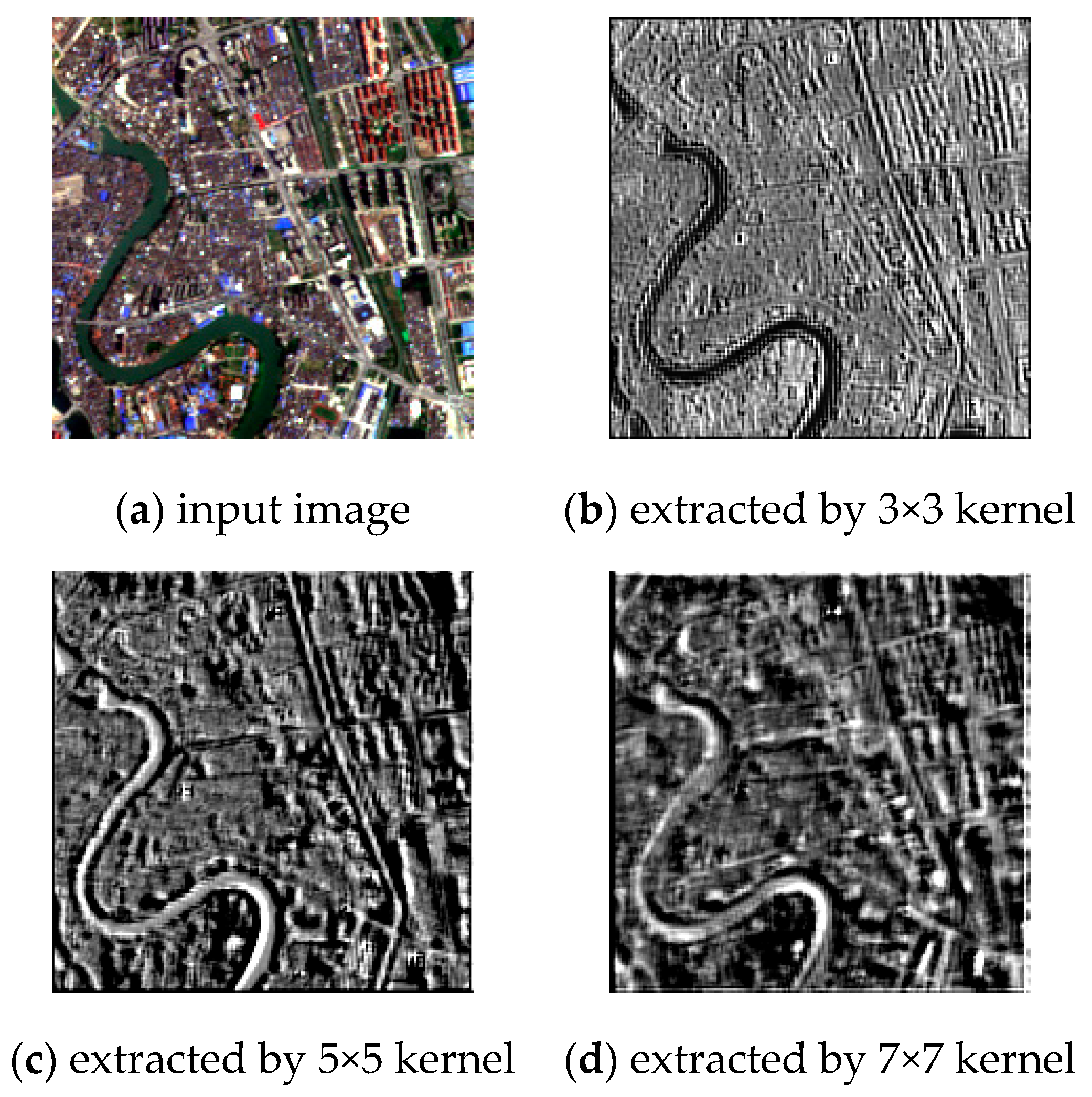
2.4. Multi-Scale Feature Extraction

For the fusion task with data at different swath widths, the HR information in the overlapping area should be introduced into the non-overlapping region. As is well known, in CNNs, the convolutional layers are used to extract features. However, the features in remote sensing images appear at different-scale levels. For example, the geometric texture of a building is at a larger scale than the texture of vegetation. Therefore, inspired by [33,34], multi-scale convolutional kernels are used to extract the features from the remote sensing images at different scales, and the feature maps are then concatenated and input into the nonlinear mapping layer below.
As shown in Figure 2, it can be seen that the different-scale convolution kernels, including 3 × 3, 5 × 5, and 7 × 7, act on the same image for the feature extraction. The image thus has different feature images after the different-scale convolution operations. It can be seen that a smaller convolution kernel (e.g., 3 × 3) focuses more on details, such as the vegetation canopy texture (i.e., the small-scale features). When using larger convolution kernels (e.g., 5 × 5 and 7 × 7), more main structures of the image are highlighted, such as the building structure, the hills, and the river. In addition, the multi-scale convolution also helps to inject HR information from the overlapping region into the non-overlapping region in the transition area between the overlapping region and the non-overlapping region. In this way, the utilization rate of the features contained in the images with different swath widths can be greatly improved, to achieve better cross-width fusion results.

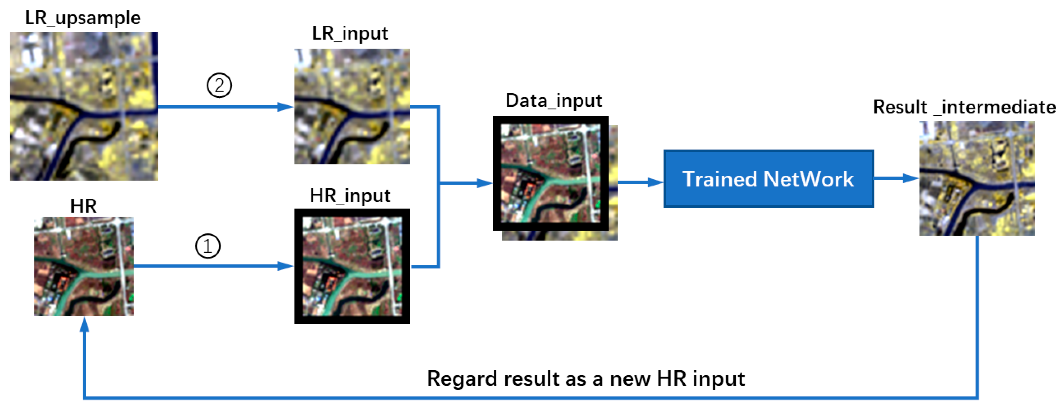
2.5. Recurrent Expanding Strategy

In this paper, for image fusion with different swath widths, the LR data are first upsampled to the same resolution as the HR image. However, due to the difference of the swath widths, the non-overlapping area lacks the available HR information. It is, therefore, difficult for the network to enhance the resolution of the transition region between the HR and LR images in the fusion process. Even the obvious resolution difference boundaries and border artifacts may appear in the fused image. When the difference in the swath width is small, less missing information is introduced, and the artifacts are not as obvious. As the difference increases, the artifacts in the results become increasingly obvious. However, the images captured by satellites vary greatly in size, which means that the missing information in the non-overlapping area is more serious. If the test dataset is notably different from the training data, the accuracy of the fusion reconstruction will be decreased.
In response to this problem, a strategy based on recurrent expansion is proposed in this paper. By using this strategy, when fusing images with different swath widths, only part of the image is fused in every iteration, which is similar to the missing data reconstruction problem. As shown in Figure 3, the input images are preprocessed and fed into the network to obtain the fusion results. At each iteration, an intermediate fused image expanded by five pixels is obtained and is regarded as a new HR image, which then undergoes expansion, cropping, concatenation, and fusion, to obtain a new fusion image in the next iteration. After multiple iterations, the WSS fusion is achieved, and the size of the high spatial resolution image is expanded by 30 or more pixels based on the difference of the swath widths between the observed images.

3. Experimental Results and Analysis

3.1. Datasets

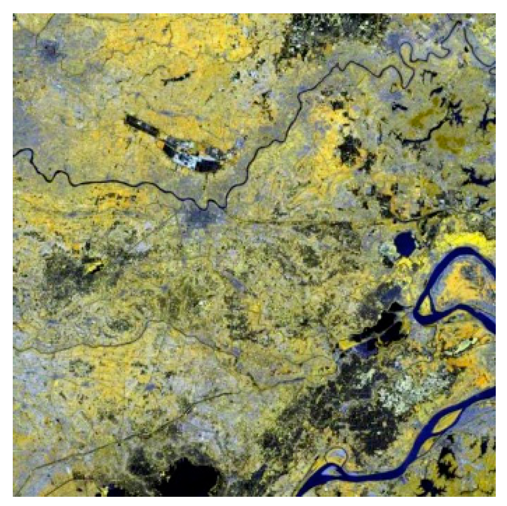
3.1.1. Training Datasets

In this set of experiments, the original data used were Sentinel-2 satellite data. The Sentinel-2 satellite, launched by the European Space Agency (ESA), covers almost all of the major territories and islands, except for the Antarctic, and is capable of providing the image data required for almost all types of research related to human life. Thirteen bands with a 290 km swath width are sensed by the Sentinel-2 satellite with a 10 day revisiting period. The spectral characteristics of the 13 bands and their resolutions are listed in Table 1; these characteristics are available for free from https://scihub.copernicus.eu/. Among them, the images of 10 m and 20 m resolution are the most widely used.
The training data selected were an image in the west of Hubei province, China acquired at September 15, 2017. The training data size was 90 × 90 km. This area is rich in water, buildings, green areas, and other ground objects, as shown in Figure 4.

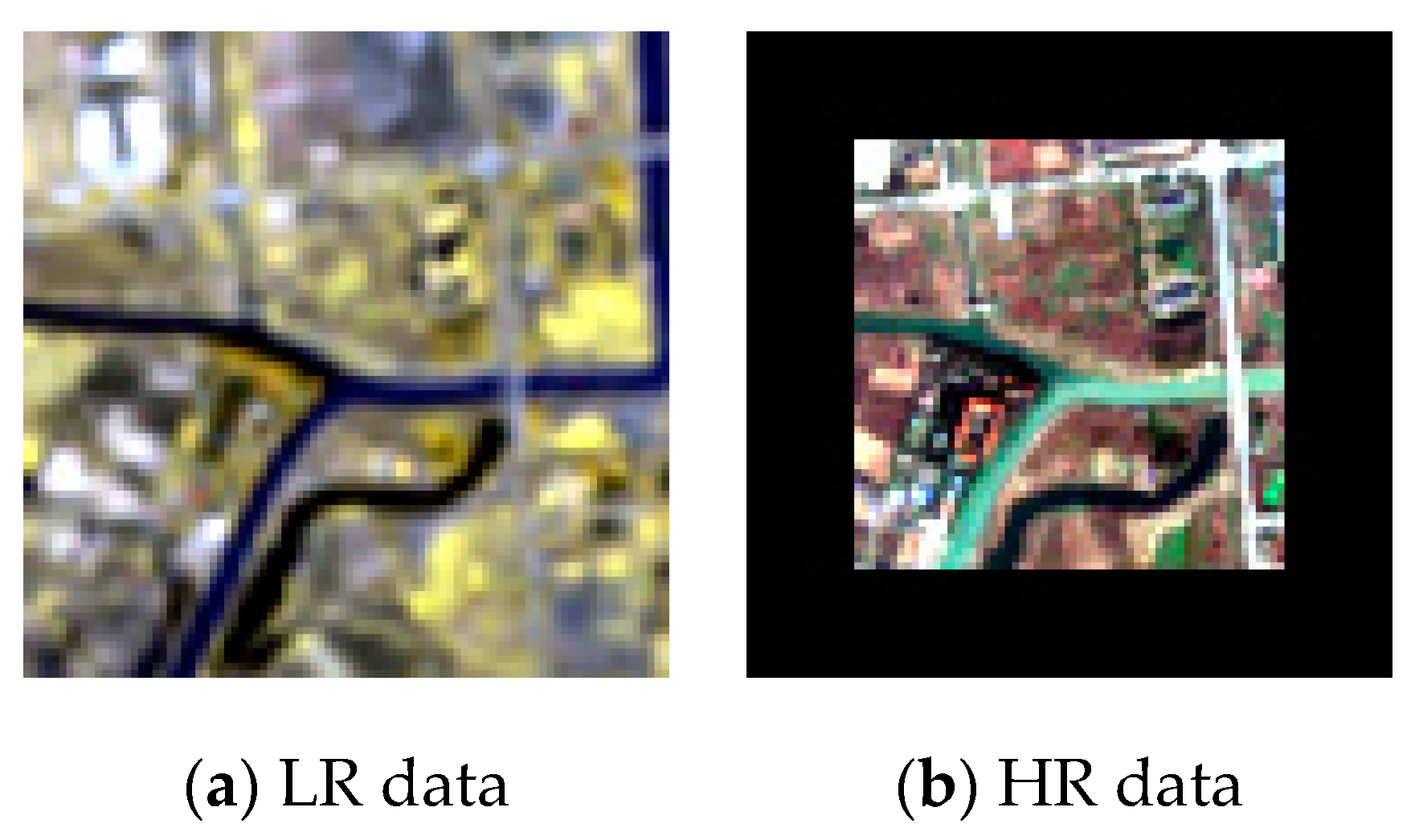
3.1.2. Test Datasets

The test data were selected from Nanjing, Jiangsu province, China, with a 900 × 900 m coverage for each image. It should be noted that there is only one swath-width imaging mode on the Sentinel-2 satellite. In order to carry out the study of WSS fusion, a different-swath-width scenario was simulated. Only four 10 m resolution bands (4B_10) and six 20 m resolution bands (6B_20) were selected. For the training data, the original image was downsampled to the 4B_20 and 6B_40 images, so that the original 6B_20 image could be used as a reference. The 6B_40 image was also upsampled to 20 m to match the 4B_20 image. The images were then cut into a series of 30 × 30 image patches. In order to simulate the different-swath-width scenario, five rows of pixels were cut out around each HR band patch. For the test data, the image was clipped into multiple 90 × 90 patches, and then 15 rows of pixels around each 20 m resolution band patch were assigned zero values, as shown in Figure 5.
The aim of the WSS fusion experiment was to obtain an HRHS image with a wide swath width.

3.2. Implementation Details

3.2.1. Parameter Setting and Network Training

Table 2 lists the network parameters of each layer of the WSSRN model. The proposed model was trained using the stochastic gradient descent algorithm as the optimization method, with a momentum of 0.9 and a learning rate of 0.1, which are obtained empirically in many deep learning methods [30].
The Caffe [35] framework was used to train the proposed WSSRN model in a Windows 10 environment, with 16 GB RAM and one Nvidia RTX 2080 GPU. The total training time cost about 3 h 50 min, which is less than VDSR with about 15 h 51 min and SRCNN with about 18 h 48 m under the same computational environment.

3.2.2. Compared Algorithms and the Quantitative Evaluation

For the image fusion of different swath widths, we mainly focus on the improvement of the spatial resolution and spectral preservation in the non-overlapping areas. Since there is no HR information introduced in the non-overlapping areas, this fusion problem can be regarded as a super-resolution problem, as described in [36]. To evaluate the effect of the spectral preservation and spatial enhancement, the bicubic algorithm, a CNN consisting of three convolutional layers (SRCNN), and a very deep convolutional network using skip connection (VDSR), were used as comparison methods. In the simulated-image experiments, the correlation coefficient (CC), peak signal-to-noise ratio (PSNR), structural similarity (SSIM), spectral angle mapper (SAM), and Erreur Relative Global Adimensionnelle de Synthèse (ERGAS) were employed as the quantitative evaluation indices. Among these indices, CC, SSIM, and PSNR are used to evaluate spatial similarity. Therefore, the higher the value, the better the result. Meanwhile, SAM is a spectral similarity index, and ERGAS is an integrated indicator, for which the lower the value, the better the result.

3.3. Sensitivity Analysis for the Overlapping Region

In WSS fusion, the HR information in the overlapping region plays an important role in the accuracy of the network. To obtain robust WSS fusion results, two factors corresponding to the relative position and size of the overlapping region were analyzed in the experiments. One was the ratio of the non-overlapping areas, called the coverage ratio, and the other was the starting pixel position of the overlapping areas of the two images, called the offset position.

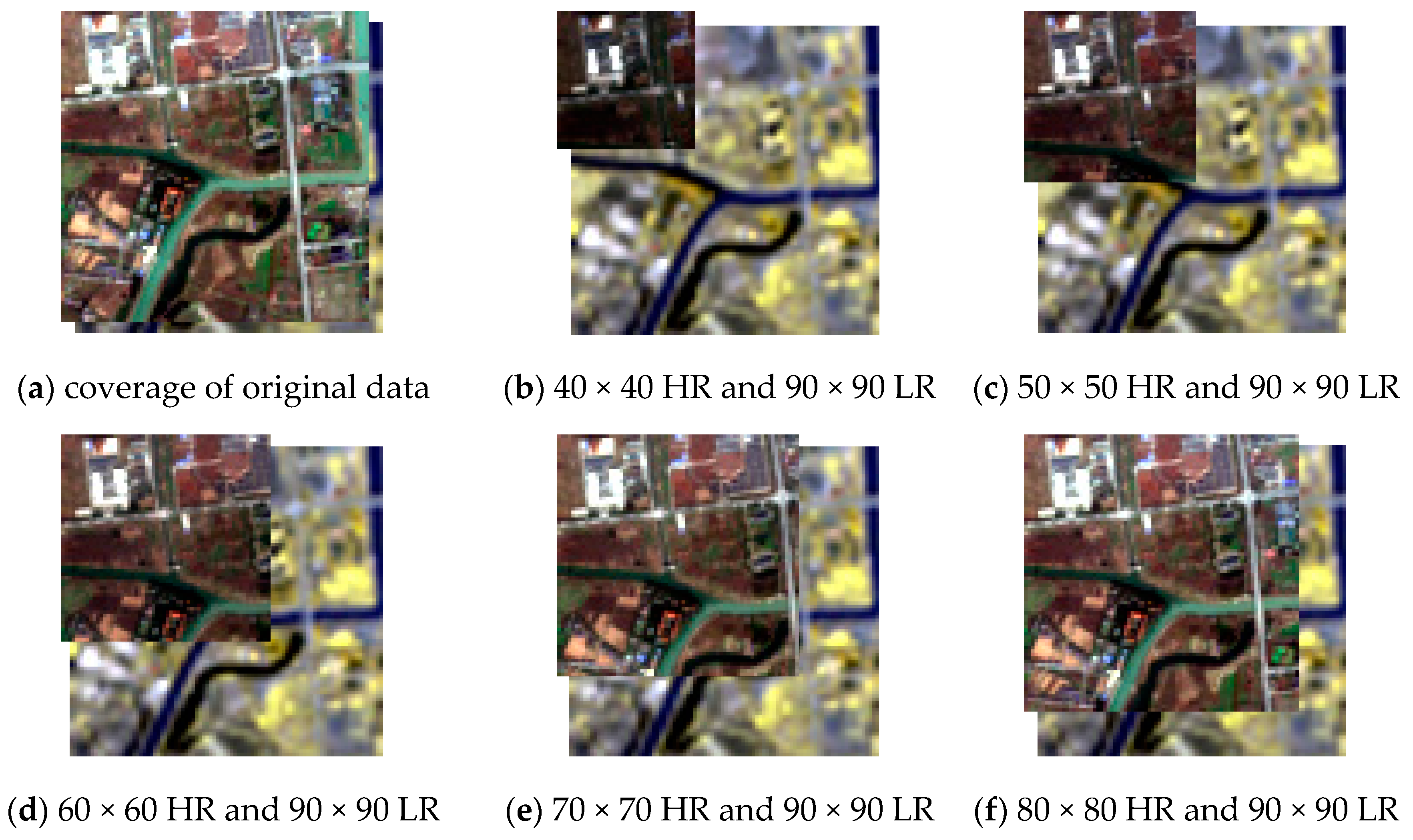
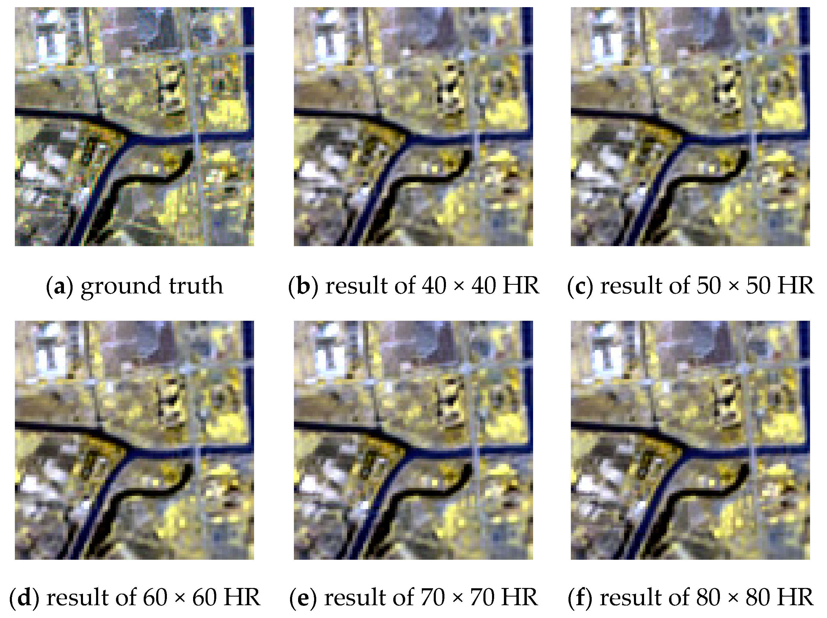
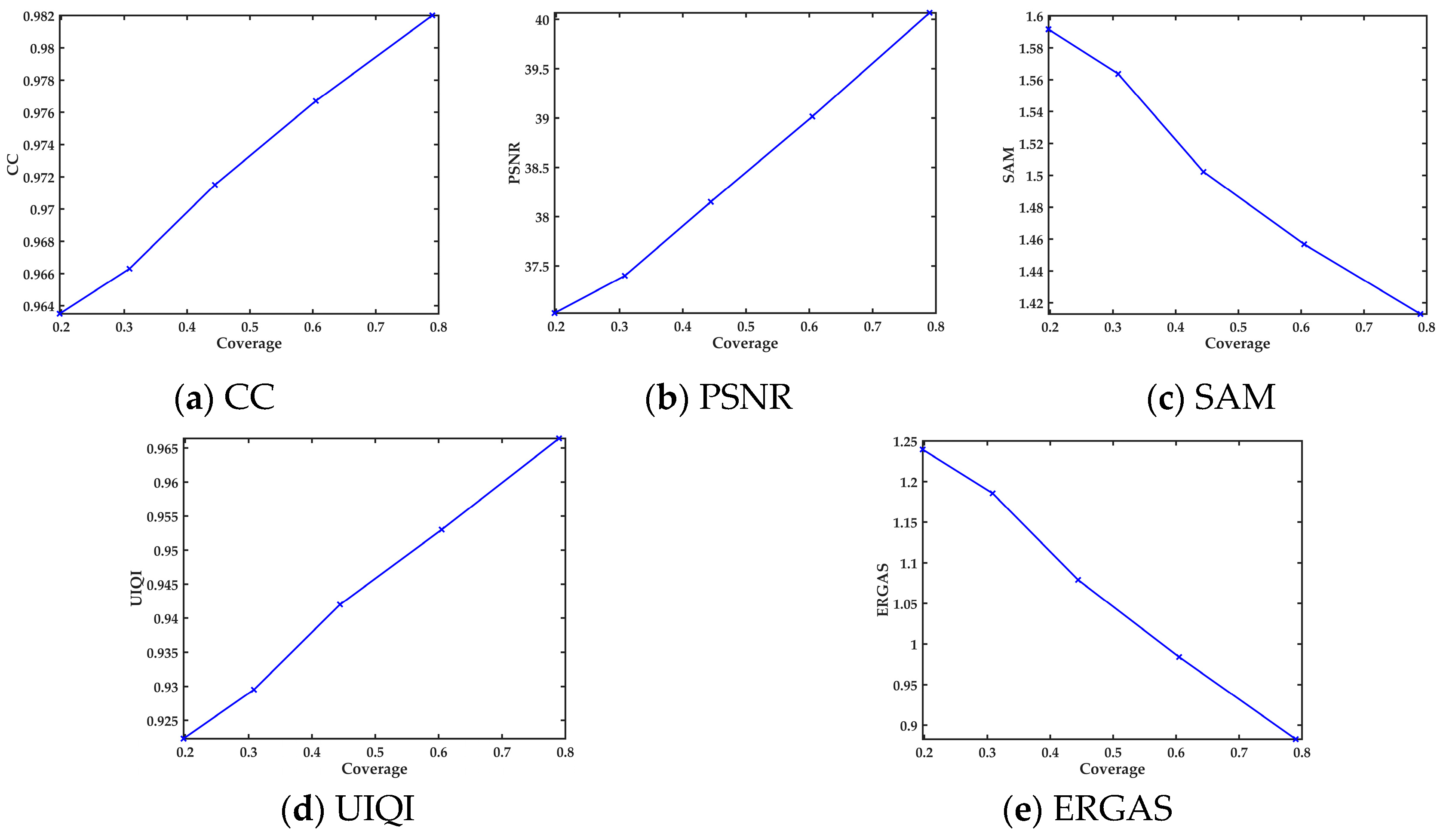
3.3.1. Coverage Ratio

In this experiment, the effect of the coverage ratio of the overlapping regions on the network fusion effect was explored. In the experimental process, the WSSRN was trained through the dataset with a coverage ratio of 0.4444. The coverage ratio is not too great or insufficient, which speeds up the network training and allows the network to learn how to handle data with different widths.
Considering the impact of the offset position, the offsets of the training data and test data were set to zero. For the test data, the HR images were clipped into images of 40 × 40 to 80 × 80, as shown in Figure 6, so the coverage ratios were, respectively, 0.1975, 0.3086, 0.4444, 0.6049, and 0.7901.
The results of the different coverage ratios are displayed in Figure 7 by false color synthesis. It can be seen from the figure that a higher coverage ratio introduces more HR information, giving the results more spatial details. The experimental results with low coverage ratio show some blurred edges in the non-overlapping area.
To better explore the influence of the coverage ratio on the fusion effect, the experimental results were quantitatively evaluated. The results of the different indices are plotted with the coverage ratio as the abscissa, as shown in Figure 8, and it can be seen that when the coverage ratio increases, the value of these evaluation indicators increases correspondingly, which shows that the fusion effect of the network is almost linearly positively correlated. When the coverage is low (e.g., 0.2 or 0.3), the rate of the fusion effect decline slows. These phenomena indicate that the fusion effect of the network is indeed related to the coverage ratio, but the relationship is almost linear.

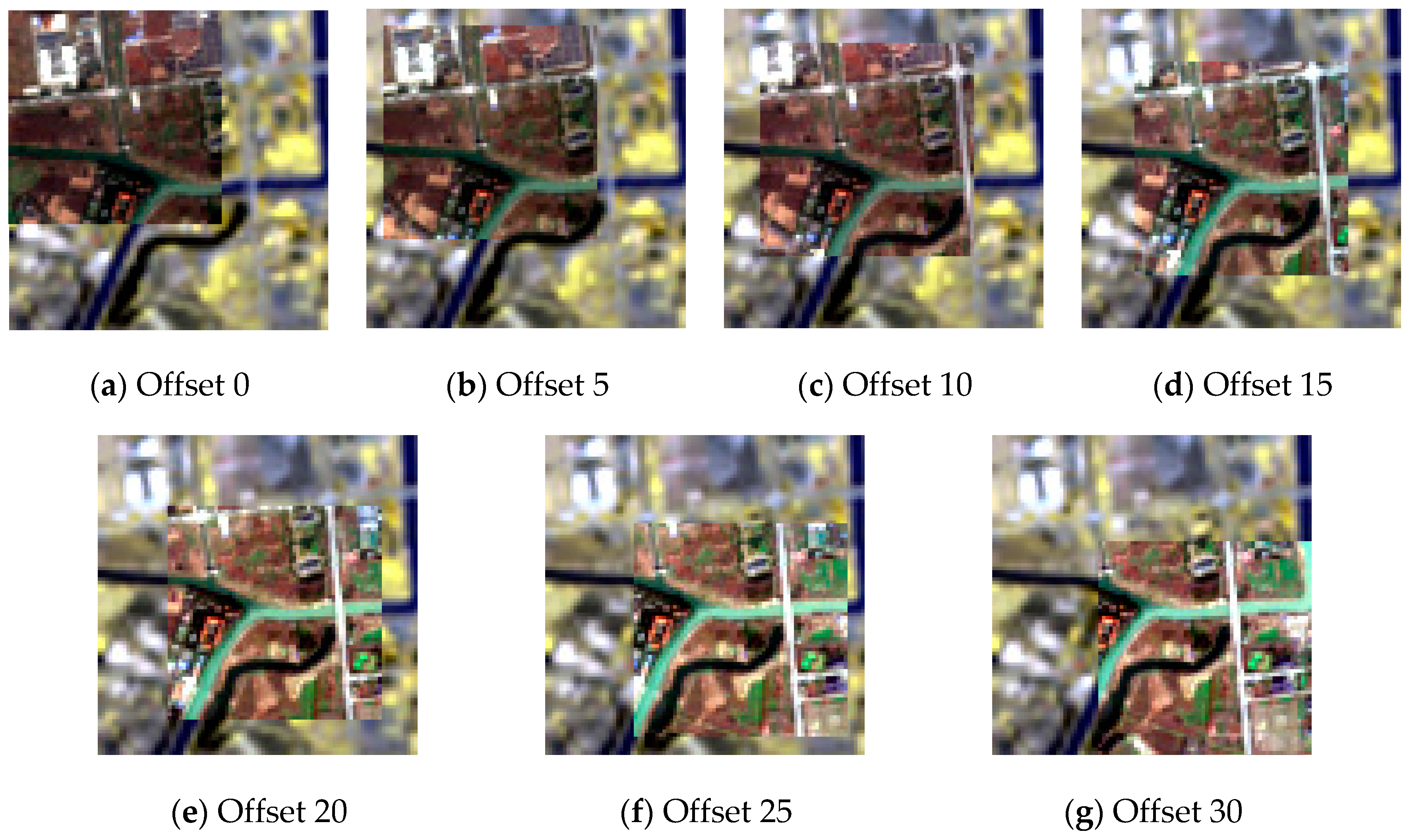
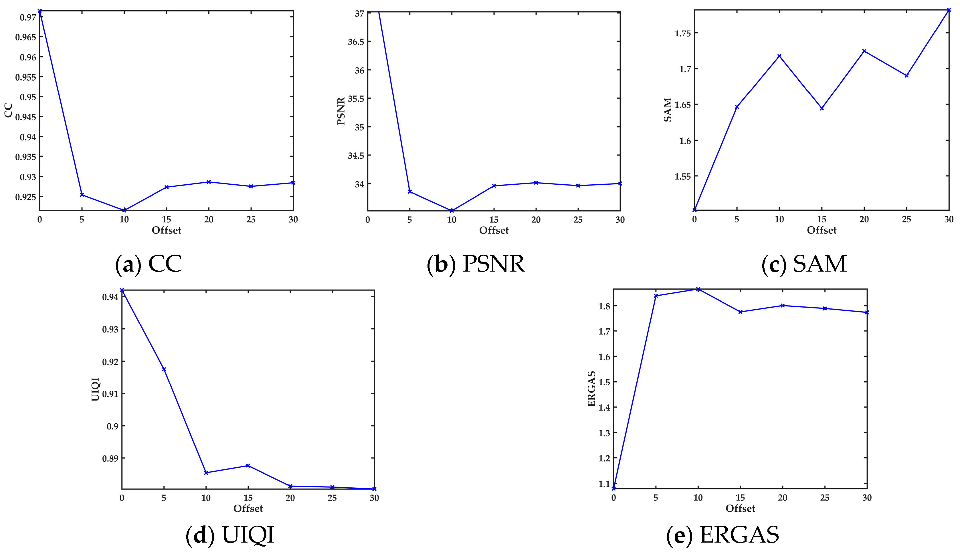
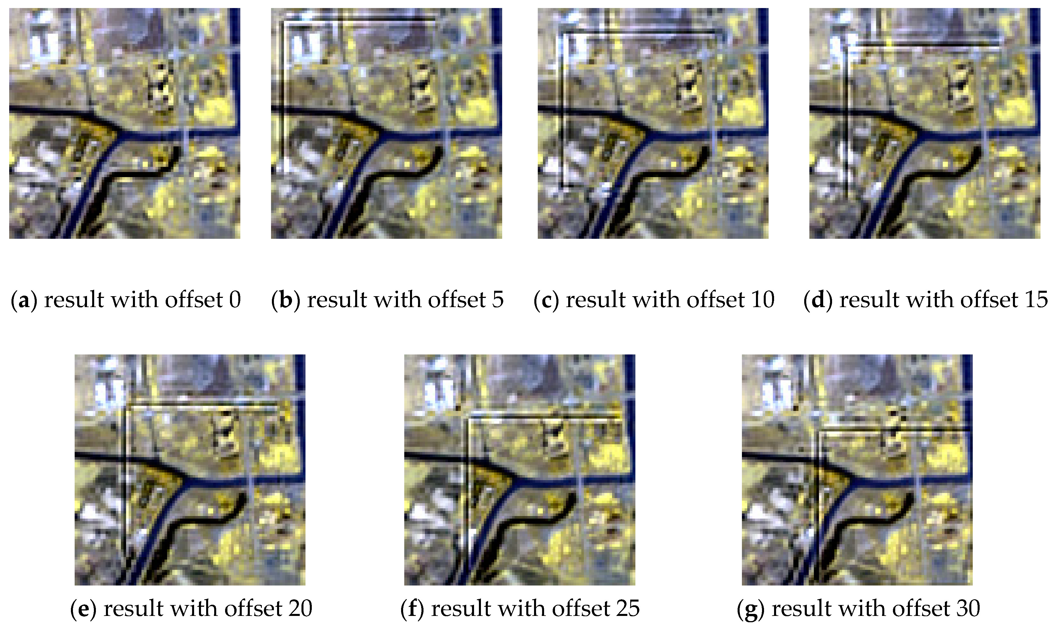
3.3.2. Offset Position

In image fusion, the utilization of the HR information in the overlapping area is expected to be maximized, so the coverage ratio of the input image is set to the maximum possible value, and thus cannot be optimized further. To obtain the best fusion effect, the offset position of the overlapping area relative to the wide-swath-width LR image was also analyzed through an experiment. In this experiment, the WSSRN model first learned the best model through the dataset with an offset position of 0.
Considering the impact of the coverage ratio, the input LR data and the HR image size were fixed. For the test data, the input LR data size was fixed as 90 × 90, and the HR image size was fixed as 60 × 60, as shown in Figure 9. For the HR image, the offset position was selected as 0, 5, 10, 15, 20, 25, and 30.
Similarly, the five quantitative evaluation indicators were again used. The results are shown in Figure 10. It can be seen that the fusion effect is diminished once the test and training data offsets are inconsistent. From the visual performance apparent in Figure 11, it is clear that, except for the experimental result with the 0 offset, there is a severe striped border effect on the other results. From this experiment, we can conclude that the CNN is very sensitive to the pixel rows of non-overlapping regions when fusing data with different swath widths. The reason for this result is that the convolution operation needs to traverse the pixels, and when the convolution kernel spans different-swath-width images, the learned mapping is inconsistent with the test mapping, resulting in the striped border artifacts in the fused result.
From the experimental results shown above, it can be seen that the fusion effect of the CNN for the data with different widths depends on the coverage ratio of the overlapping areas and the offset position in the training data. Furthermore, the influence on the fusion effect of the coverage ratio increases linearly and steadily, which will never lead to the unexpected white borders or details in the image, whereas the change caused by the offset position may result in spatial artifacts. Therefore, the offset position can be regarded as the more critical factor for the network proposed in this paper. During the training, the offset position can be increased to fuse more areas at a time. However, this has high hardware requirements and greatly increases the network optimization time. To give the fusion network a better generalization ability, a fixed number of pixels are reconstructed each time when the fusion is carried out by the proposed recurrent expanding strategy described in Section 2.5, which ensures that the offset of the training and the test data is the same.

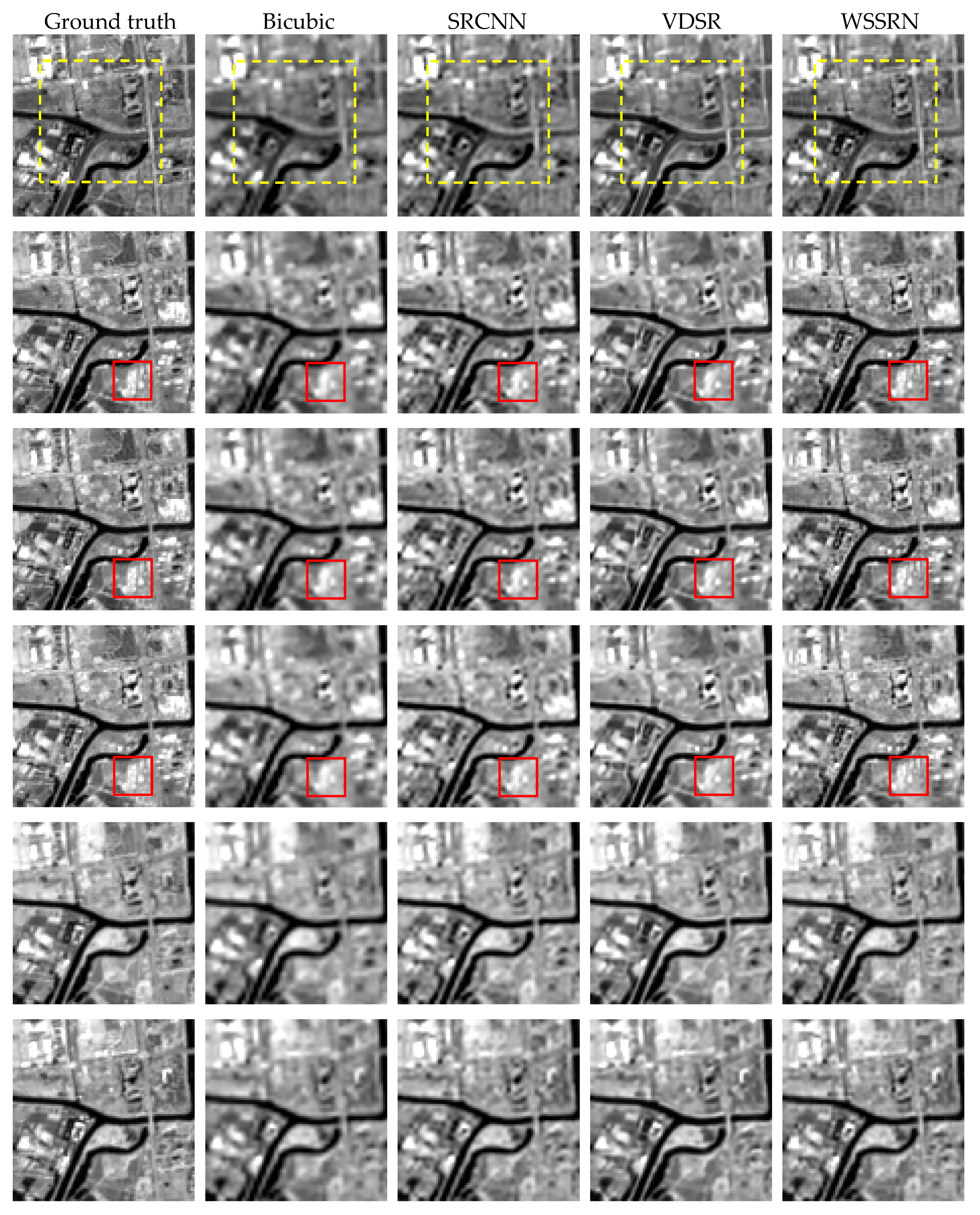
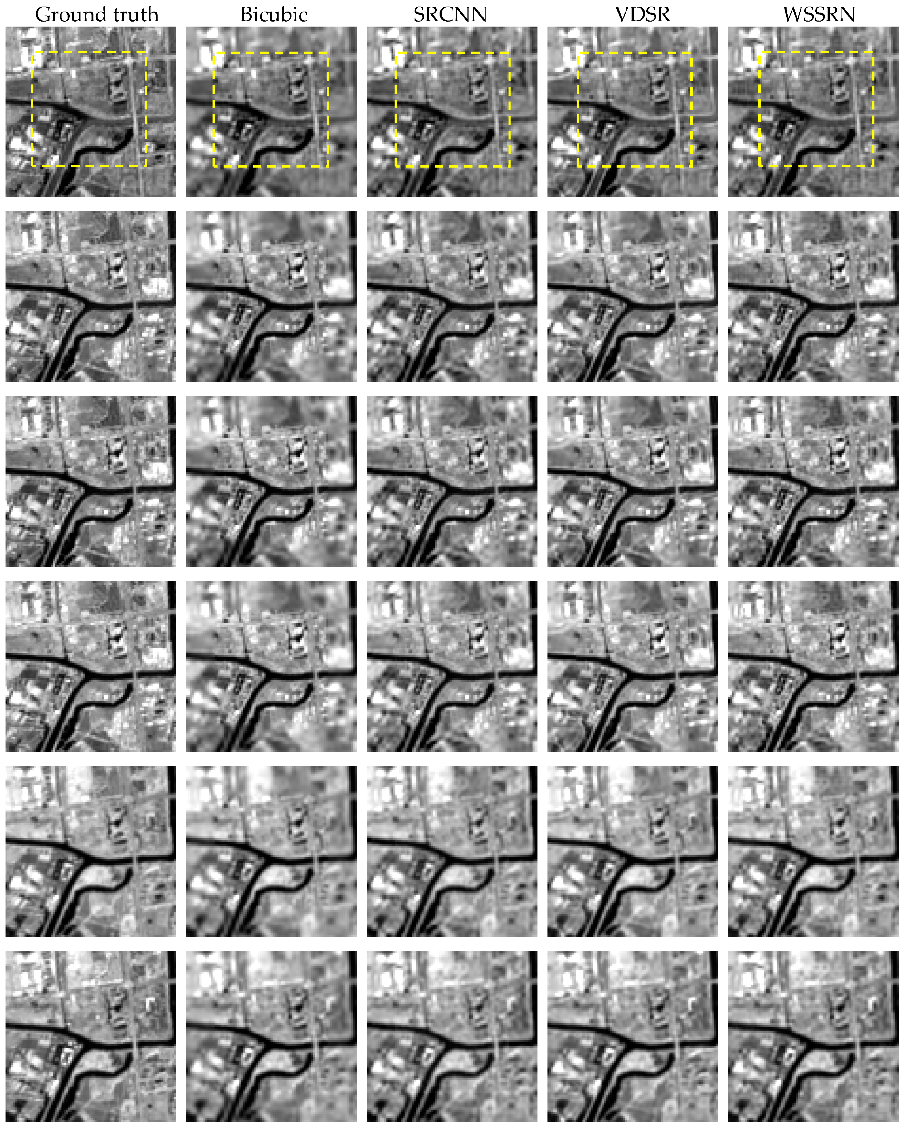
3.4. Simulated Experiment

In order to quantitatively compare the proposed WSSRN model with the other methods, the original Sentinel-2 data were downsampled to a 4 m resolution and a 20 m resolution. In this way, the simulated experiment involved obtaining a 90 × 90 six-band image with a 20 m resolution by fusing a 90 × 90 six-band image with a 40 m resolution and a 60 × 60 four-band image with a 20 m resolution. The original 90 × 90 six-band image with a 20 m resolution could then be used as a reference for the quantitative assessment.
The results of the different methods are shown in Figure 12 (the overlapping area is framed by a dotted yellow line). It can be seen that SRCNN and VDSR show a certain effect in improving the spatial resolution in the visual performance, but their effect on high-brightness areas, as framed by red, is rather poor, and they cannot be well enhanced. There is also a visual sharpness that does not conform to the real situation. The fusion effect of the WSSRN model proposed in this paper is the best of all methods. More texture information is fused into the wide-swath-width image through the multi-scale feature extraction, and in the transition zone between the HR and LR images, due to the proposed recurrent expanding strategy, the acute change in resolution is alleviated. The results of the proposed WSSRN model are also more visually natural.
The quality of the fusion improved after using the WSSRN method (Table 3). For both spatial similarity and spectral preservation, the fusion framework proposed in this paper has certain advantages. The worst effect of all the methods is found for the interpolation method. In addition, due to the weak generalization ability of the Sentinel-2 imagery, SRCNN introduces a sharpening effect in the highlighted area.

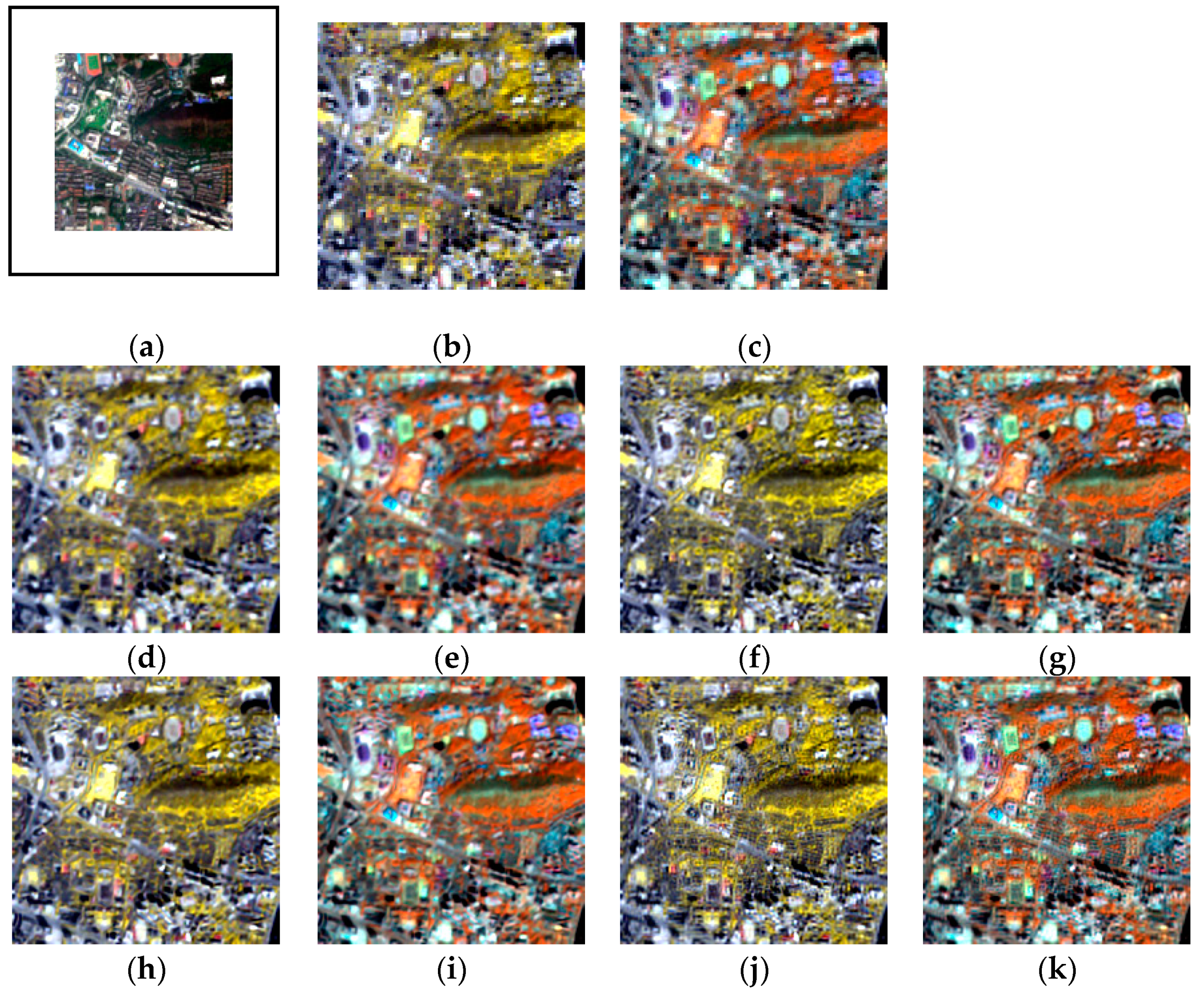
3.5. Real-Data Experiment

The WSS fusion was also implemented in the real resolution of Sentinel-2 data by simulating a multi-width scenario. We get a HRLS data covering a 1.2 × 1.2 km area and an LRHS data covering a 2 × 2 km area in Wuhan city, Hubei province, China out of the training data and the trained network, using a 5 pixel offset position and a 0.4444 coverage ratio. For the real-data experiment, since Sentinel-2 data with a 10 m resolution cannot be acquired, a quantitative assessment is impossible, and only a rough judgment on the fusion effect of the image can be made from the visual performance. Figure 13 shows the change of the false-color synthesis and grayscale image of three 20 m resolution bands with the worst fusion effect before and after the real-data experiment.
Because VDSR is much better than SRCNN in its super-resolution, only VDSR is compared with the proposed WSSRN model. Comparing Figure 13a,f, it can be seen that the swath width of the narrow-swath-width image has increased after the fusion, and, at the same time, the spectral resolution of the new HR image is also improved, which is consistent with the original LR multispectral image (original band 5, band 6, band 7, band 8a, band 11, and band 12). As can be seen from the six bands before and after fusion, the spatial resolution of the fused image is greatly enhanced. Looking at the results of band 8a, band 11, and band 12, it can be found that the spatial enhancement is obvious, not only in the central overlapping area, but also in the non-overlapping area. Compared with Figure 13d,e, the result of WSSRN contains more texture information than the result of VDSR. Overall, the real-data experiment confirms that the proposed WSSRN model and recurrent expanding strategy can effectively consider the constraints between the spectra, space, and swath width, and can fuse them simultaneously to obtain a good result.

4. Discussion

The traditional method of using LRHS data with wide swath width and the HRLS data with narrow swath width is that the overlapped areas of data can be fused by spatial–spectral fusion first, and then the non-overlapped areas can be reconstructed by super-resolution. Finally, they are spliced together to obtain HRHS data. In this way, it is possible to achieve the WSS fusion and utilize all HR and LR data at the same time, but it is not clear whether the maximum utilization of the HR data has been achieved.
To discuss whether the WSSRN can use HR data to enhance the spatial resolution of non-overlapping areas while fusing the overlapping areas compared to traditional splicing methods, the central areas of the super resolution methods were replaced by the central area of our WSSRN, because HR data only covers central areas, which are shown in Figure 14.
The overlapping area is framed by a dotted yellow line. Due to the insufficient extraction of spatial detail information, when the overlapping region is replaced with the image patch with rich HR information, the results fused by the bicubic, SRCNN, and VDSR methods show a poor fusion effect in the surrounding area. In addition, the results of VDSR show a great difference in the fusion effect of the different bands, so it is difficult to use the data generated by this method in practical applications. However, the performance of the WSSRN is balanced.
As shown in Table 4, we can see that the indices for VDSR and SRCNN are significantly improved after replacement, indicating that the central part contains enough HR information. It is, however, clear from the evaluation that the result of the proposed method are still better than those of the other algorithms, which indicates that the introduction of multi-scale feature extraction combined with the recurrent expanding strategy can effectively inject the HR information of the central overlapping area into the surrounding area to improve the final fusion results. From the experimental results, it can be concluded that the proposed WSSRN model can effectively fuse data with different widths, different spatial resolutions, and different spectral resolutions.

5. Conclusions

In this paper, a multi-scale residual CNN was proposed to deal with remote sensing image fusion problems with different swath widths. This represents an early attempt to incorporate swath width, spatial resolution, and spectral resolution into one network to simultaneously achieve multi-band fusion and swath-width enhancement. In this process, how the CNN deals with the sensitivity of the variables between different-width data was explored by experiments, and then a step-by-step reconstruction method based on a recurrent expanding strategy was proposed. By exploiting and transferring the HR information of the central overlapping area from the different swath-width images, the proposed framework can effectively improve the resolution of the non-overlapping regions. The experiments showed that the WSSRN can achieve a better spatial resolution improvement in the surrounding non-overlapping area without HR information than the current single-image super-resolution methods.
Moreover, there are several limits in the proposed WSSRN. Although the spatial resolution of the surrounding non-overlapping area without HR information can be enhanced by WSSRN, it still seems to be blurred, and if the spatial resolution difference between the HR data and LR data is too large, the proposed WSSRN will be greatly affected. In our future work, we will consider introducing an attention module into the neural network and combining a variational model with deep learning to further improve the spatial enhancement.

Author Contributions

Conceptualization, H.J., L.J. and Y.Q.; Formal analysis, H.J.; Funding acquisition, L.J.; Investigation, H.J.; Methodology, H.J. and L.J.; Project administration, L.J., Y.Q. and S.H.; Resources, L.J. and Y.Q.; Supervision, L.J., Y.Q., L.H. and S.H.; Validation, H.J.; Writing—original draft, H.J.; Writing—review and editing, L.J., Y.Q., L.H. and S.H. All authors read and approved the final manuscript.

Funding

This research was funded by National Key R&D Program of China, grant number 2017YFA0604402, National Natural Science Foundation of China, grant number 61971319, 41701400 and 41922008.

Acknowledgments

We are grateful for the free and open source Sentinel-2 data provided by ESA and the author of VDSR method.

Conflicts of Interest

The authors declare no conflict of interest.

References

  1. Li, J.; Liu, X.; Yuan, Q.; Shen, H.; Zhang, L. Antinoise Hyperspectral Image Fusion by Mining Tensor Low-Multilinear-Rank and Variational Properties. IEEE Trans. Geosci. Remote Sens. 2019. [Google Scholar] [CrossRef]
  2. Gillespie, A.R.; Kahle, A.B.; Walker, R.E. Color enhancement of highly correlated images. 2. Channel ratio and chromaticity transformation techniques. Remote Sens. Environ. 1987, 22, 343–365. [Google Scholar] [CrossRef]
  3. Chavez, P.S.; Kwarteng, A.Y. Extracting spectral contrast in Landsat thematic mapper image data using selective principal component analysis. Photogramm. Eng. Remote Sens. 1989, 55, 339–348. [Google Scholar]
  4. Tu, T.M.; Huang, P.S.; Hung, C.L.; Chang, C.P. A fast intensity hue-saturation fusion technique with spectral adjustment for IKONOS imagery. IEEE Geosci. Remote Sens. Lett. 2004, 1, 309–312. [Google Scholar] [CrossRef]
  5. Laben, C.A.; Brower, B.V. Process for enhancing the spatial resolution of multispectral imagery using pan-sharpening. U.S. Patents 6,011,875, 4 January 2000. [Google Scholar]
  6. Aiazzi, B.; Alparone, L.; Baronti, S.; Garzelli, A. Context-driven fusion of high spatial and spectral resolution images based on oversampled multiresolution analysis. IEEE Trans. Geosci. Remote Sens. 2002, 40, 2300–2312. [Google Scholar] [CrossRef]
  7. Nencini, F.; Garzelli, A.; Baronti, S.; Alparone, L. Remote sensing image fusion using the curvelet transform. Inf. Fusion 2007, 8, 143–156. [Google Scholar] [CrossRef]
  8. Aiazzi, B.; Alparone, L.; Baronti, S.; Garzelli, A.; Selva, M. MTF tailored multiscale fusion of high-resolution MS and pan imagery. Photogramm. Eng. Remote Sens. 2006, 72, 591–596. [Google Scholar] [CrossRef]
  9. Palsson, F.; Sveinsson, J.R.; Ulfarsson, M.O.; Benediktsson, J.A. MTF-based deblurring using a wiener filter for CS and MRA pansharpening methods. IEEE J. Sel. Top. Appl. Earth Obs. Remote Sens. 2016, 9, 2255–2269. [Google Scholar] [CrossRef]
  10. Liu, J.G. Smoothing filter-based intensity modulation: A spectral preserve image fusion technique for improving spatial details. Int. J. Remote Sens. 2000, 21, 3461–3472. [Google Scholar] [CrossRef]
  11. Garzelli, A.; Nencini, F.; Capobianco, L. Optimal MMSE pan sharpening of very high resolution multispectral images. IEEE Trans. Geosci. Remote Sens. 2008, 46, 228–236. [Google Scholar] [CrossRef]
  12. Garzelli, A. Pansharpening of multispectral images based on nonlocal parameter optimization. IEEE Trans. Geosci. Remote Sens. 2015, 53, 2096–2107. [Google Scholar] [CrossRef]
  13. Fasbender, D.; Radoux, J.; Bogaert, P. Bayesian data fusion for adaptable image pansharpening. IEEE Trans. Geosci. Remote Sens. 2008, 46, 1847–1857. [Google Scholar] [CrossRef]
  14. Zhang, L.; Shen, H.; Gong, W.; Zhang, H. Adjustable model-based fusion method for multispectral and panchromatic images. IEEE Trans. Syst. Man Cybern. B Cybern. 2012, 42, 1693–1704. [Google Scholar] [CrossRef]
  15. Palsson, F.; Sveinsson, J.R.; Ulfarsson, M.O. A new pansharpening algorithm based on total variation. IEEE Geosci. Remote Sens. Lett. 2014, 11, 318–322. [Google Scholar] [CrossRef]
  16. Shen, H.; Meng, X.; Zhang, L. An integrated framework for the spatio–temporal–spectral fusion of remote sensing images. IEEE Trans. Geosci. Remote Sens. 2016, 54, 7135–7148. [Google Scholar] [CrossRef]
  17. Jiang, C.; Zhang, H.; Shen, H.; Zhang, L. A practical compressed sensing-based pan-sharpening method. IEEE Geosci. Remote Sens. Lett. 2012, 9, 629–633. [Google Scholar] [CrossRef]
  18. Song, H.; Huang, B.; Liu, Q.; Zhang, K. Improving the Spatial Resolution of Landsat TM/ETM+ Through Fusion With SPOT5 Images via Learning-Based Super-Resolution. IEEE Trans. Geosci. Remote Sens. 2015, 53, 1195–1204. [Google Scholar] [CrossRef]
  19. Huang, W.; Xiao, L.; Wei, Z.; Liu, H.; Tang, S. A New Pan-Sharpening Method With Deep Neural Networks. IEEE Geosci. Remote Sens. Lett. 2015, 12, 1037–1041. [Google Scholar] [CrossRef]
  20. Masi, G.; Cozzolino, D.; Verdoliva, L.; Scarpa, G. Pansharpening by convolutional neural networks. Remote Sens. 2016, 8, 594. [Google Scholar] [CrossRef]
  21. Yuan, Q.; Wei, Y.; Meng, X.; Shen, H.; Zhang, L. A Multiscale and Multidepth Convolutional Neural Network for Remote Sensing Imagery Pan-Sharpening. IEEE J. Sel. Top. Appl. Earth Observ. Remote Sens. 2018, 11, 978–989. [Google Scholar] [CrossRef]
  22. Wei, Y.; Yuan, Q.; Shen, H.; Zhang, L. Boosting the Accuracy of Multispectral Image Pansharpening by Learning a Deep Residual Network. IEEE Geosci. Remote Sens. Lett. 2017, 14, 1795–1799. [Google Scholar] [CrossRef] [Green Version]
  23. Palsson, F.; Sveinsson, J.; Ulfarsson, M. Sentinel-2 Image Fusion Using a Deep Residual Network. Remote Sens. 2018, 10, 1290. [Google Scholar] [CrossRef]
  24. Wang, Q.; Shi, W.; Li, Z.; Atkinson, P.M. Fusion of Sentinel-2 images. Remote Sens. Environ. 2016, 187, 241–252. [Google Scholar] [CrossRef] [Green Version]
  25. Wang, Q.; Blackburn, G.A.; Onojeghuo, A.O.; Dash, J.; Zhou, L.; Zhang, Y.; Atkinson, P.M. Fusion of Landsat 8 OLI and Sentinel-2 MSI Data. IEEE Trans. Geosci. Remote Sens. 2017, 55, 3885–3899. [Google Scholar] [CrossRef] [Green Version]
  26. Wang, Q.; Shi, W.; Atkinson, P.M.; Zhao, Y. Downscaling MODIS images with area-to-point regression kriging. Remote Sens. Environ. 2015, 166, 191–204. [Google Scholar] [CrossRef]
  27. Yi, C.; Zhao, Y.; Chan, J.C. Hyperspectral Image Super-Resolution Based on Spatial and Spectral Correlation Fusion. IEEE Trans. Geosci. Remote Sens. 2018, 56, 4165–4177. [Google Scholar] [CrossRef]
  28. Sun, X.; Zhang, L.; Yang, H.; Wu, T.; Cen, Y.; Guo, Y. Enhancement of Spectral Resolution for Remotely Sensed Multispectral Image. IEEE J. Sel. Top. Appl. Earth Observ. Remote Sens. 2015, 8, 2198–2211. [Google Scholar] [CrossRef]
  29. Dong, C.; Loy, C.C.; He, K.; Tang, X. Image super-resolution using deep convolutional networks. IEEE Trans. Pattern Anal. Mach. Intell. 2016, 38, 295–307. [Google Scholar] [CrossRef]
  30. Kim, J.; Lee, J.K.; Lee, K.M. Accurate Image Super-Resolution Using Very Deep Convolutional Networks. In Proceedings of the IEEE Conference on Computer Vision and Pattern Recognition, Las Vegas, NV, USA, 26 June–1 July 2016; pp. 1646–1654. [Google Scholar]
  31. Lanaras, C.; Bioucas-Dias, J.; Galliani, S.; Baltsavias, E.; Schindler, K. Super-resolution of Sentinel-2 images: Learning a globally applicable deep neural network. ISPRS J. Photogramm. Remote Sens. 2018, 146, 305–319. [Google Scholar] [CrossRef] [Green Version]
  32. He, K.; Zhang, X.; Ren, S.; Sun, J. Deep residual learning for image recognition. In Proceedings of the IEEE Conference on Computer Vision and Pattern Recognition, Las Vegas, NV, USA, 26 June–1 July 2016; pp. 770–778. [Google Scholar]
  33. Zhang, Q.; Yuan, Q.; Zeng, C.; Li, X.; Wei, Y. Missing data reconstruction in remote sensing image with a unified spatial-temporal-spectral deep convolutional neural network. IEEE Trans. Geosci. Remote Sens. 2018, 56, 4274–4288. [Google Scholar] [CrossRef]
  34. Yuan, Q.; Zhang, Q.; Li, J.; Shen, H.; Zhang, L. Hyperspectral image denoising employing a spatial-spectral deep residual convolutional neural network. IEEE Trans. Geosci. Remote Sens. 2019, 57, 1205–1218. [Google Scholar] [CrossRef]
  35. Jia, Y.; Shelhamer, E.; Donahue, J.; Karayev, S.; Long, J.; Girshick, R.; Guadarrama, S.; Darrell, T. Caffe: Convolutional architecture for fast feature embedding. In Proceedings of the 22nd ACM International Conference on Multimedia, Orlando, FL, USA, 3–7 November 2014; pp. 675–678. [Google Scholar]
  36. Li, J.; Yuan, Q.; Shen, H.; Meng, X.; Zhang, L. Hyperspectral Image Super-Resolution by Spectral Mixture Analysis and Spatial–Spectral Group Sparsity. IEEE Geosci. Remote Sens. Lett. 2016, 13, 1250–1254. [Google Scholar] [CrossRef]
Figure 1. The architecture of the proposed width-space-spectrum residual network (WSSRN) model.
Remotesensing 11 02203 g001
Figure 2. The feature maps extracted by the multiple-scale convolution kernels.
Remotesensing 11 02203 g002
Figure 3. The process of the recurrent expanding strategy. Step 1: Expand the high spatial resolution (HR) data by several pixels assigned to 0. Step 2: Crop the low spatial resolution (LR)_upsample data to the same size and same coverage as the HR_input.
Remotesensing 11 02203 g003
Figure 4. Coverage of the training data.
Remotesensing 11 02203 g004
Figure 5. Coverage of the test data.
Remotesensing 11 02203 g005
Figure 6. The data coverage in the coverage ratio experiment.
Remotesensing 11 02203 g006
Figure 7. The results of the coverage ratio experiment.
Remotesensing 11 02203 g007
Figure 8. Quantitative evaluation results for different offset positions.
Remotesensing 11 02203 g008
Figure 9. The data coverage in the offset position experiment.
Remotesensing 11 02203 g009
Figure 10. Quantitative evaluation results for different offset positions.
Remotesensing 11 02203 g010
Figure 11. Visual performance with different offsets.
Remotesensing 11 02203 g011
Figure 12. Visual performance for the simulated experiment. Each row belongs to one band. From top to bottom: band 5, band 6, band 7, band 8a, band 11, and band 12.
Remotesensing 11 02203 g012
Figure 13. Visual performance before and after fusion. (a) The narrow-swath-width HR data. (b) False-color synthesis of band 5, band 6, and band 7 before fusion. (c) False-color synthesis of band 8a, band 11, and band 12 before fusion. (d,e) The results of bicubic. (f,g) The results of SRCNN. (h,i) The results of VDSR. (j,k) The results of WSSRN.
Remotesensing 11 02203 g013
Figure 14. Visual performance after the replacement. Each row belongs to one band. From top to bottom: band 5, band 6, band 7, band 8a, band 11, and band 12.
Remotesensing 11 02203 g014
Table 1. The band details for Sentinel-2.
BandB1B2B3B4B5B6B7B8B8aB9B10B11B12
Wavelength (nm)443490560665705740783842865945138016102190
Width (nm)2065353015152011520203090180
Resolution (m)60101010202020102060602020
Table 2. The network configuration of the WSSRN model.
Configuration
Layer 1_1
Layer 1_2
Layer 1_3
Conv + ReLU: size=3, stride=1, pad=1
Conv + ReLU: size=5, stride=1, pad=2
Conv + ReLU: size=7, stride=1, pad=3
9 LayersConv + ReLU: size=7, stride=1, pad=3
Layer 11Conv + ReLU: size=3, stride=1, pad=1
Table 3. Quantitative evaluation for the simulated experiment.
MethodIndexBand 5Band 6Band 7Band 8aBand 11Band 12
BicubicCC0.940.940.940.940.970.96
PSNR35.1132.0630.8429.7831.2431.64
SSIM0.890.860.850.840.890.88
SAM1.76
ERGAS1.55
SRCNNCC0.950.950.950.960.980.97
PSNR35.2732.8031.6730.6431.9231.24
SSIM0.920.900.890.890.930.92
SAM2.18
ERGAS1.4868
VDSRCC0.970.960.960.960.980.98
PSNR37.3534.3032.8931.9534.5034.62
SSIM0.930.920.910.910.940.93
SAM1.48
ERGAS1.15
WSSRNCC0.970.970.970.970.990.98
PSNR37.2334.9833.7032.8834.7134.60
SSIM0.950.940.940.940.950.94
SAM1.57
ERGAS1.09
Table 4. Quantitative evaluation for the simulated experiment with the same center image.
MethodIndexBand 5Band 6Band 7Band 8aBand 11Band 12
BicubicCC0.95870.96470.96420.96740.98110.9735
PSNR36.5133.8932.6931.7733.1633.39
SSIM0.93730.92540.91940.91730.93720.9254
SAM1.59
ERGAS1.25
SRCNNCC0.96240.96970.97050.97270.98420.9748
PSNR36.5734.3133.1232.1233.3732.92
SSIM0.94560.93920.93590.93450.95010.9384
SAM1.85
ERGAS1.24
VDSRCC0.96560.97150.97200.97440.98640.9789
PSNR37.3534.6233.6632.7734.6634.45
SSIM0.94720.94120.93660.93520.95350.9415
SAM1.60
ERGAS1.11
WSSRNCC0.96460.97240.97190.97470.98680.9796
PSNR37.2334.9833.7032.8834.7134.60
SSIM0.94570.94210.93670.93620.95380.9423
SAM1.57
ERGAS1.09

