Article

The Potential of Open Geodata for Automated Large-Scale Land Use and Land Cover Classification

1
German Remote Sensing Data Center, Earth Observation Center, German Aerospace Center, 82234 Wessling, Germany
2
Daimler Insurance Services GmbH, 70469 Stuttgart, Germany
3
Independent scholar, 80686 Munich, Germany
*
Author to whom correspondence should be addressed.
Remote Sens. 2019, 11(19), 2249; https://0-doi-org.brum.beds.ac.uk/10.3390/rs11192249
Submission received: 23 August 2019 / Revised: 21 September 2019 / Accepted: 21 September 2019 / Published: 27 September 2019

Abstract

:
This study examines the potential of open geodata sets and multitemporal Landsat satellite data as the basis for the automated generation of land use and land cover (LU/LC) information at large scales. In total, six openly available pan-European geodata sets, i.e., CORINE, Natura 2000, Riparian Zones, Urban Atlas, OpenStreetMap, and LUCAS in combination with about 1500 Landsat-7/8 scenes were used to generate land use and land cover information for three large-scale focus regions in Europe using the TimeTools processing framework. This fully automated preprocessing chain integrates data acquisition, radiometric, atmospheric and topographic correction, spectral–temporal feature extraction, as well as supervised classification based on a random forest classifier. In addition to the evaluation of the six different geodata sets and their combinations for automated training data generation, aspects such as spatial sampling strategies, inter and intraclass homogeneity of training data, as well as the effects of additional features, such as topography and texture metrics are evaluated. In particular, the CORINE data set showed, with up to 70% overall accuracy, high potential as a source for deriving dominant LU/LC information with minimal manual effort. The intraclass homogeneity within the training data set was of central relevance for improving the quality of the results. The high potential of the proposed approach was corroborated through a comparison with two similar LU/LC data sets, i.e., GlobeLand30 and the Copernicus High Resolution Layers. While similar accuracy levels could be observed for the latter, for the former, accuracy was considerable lower by about 12–24%.

Graphical Abstract

1. Introduction

Land is a limited resource. Particularly in Europe, land resources are scarce and as a result, conflicting land uses for settlement, production systems, and infrastructure arise. Information about land use and land cover (LU/LC) derived from satellite data is therefore becoming increasingly important for environmental monitoring to support decision-making and reporting processes [1,2,3,4].
In Europe, the free and open products and services that the Copernicus Land Monitoring Service of the European Commission provides, constitute an important source to facilitate the sustainable management of the land and its usage [5,6]. However, the Copernicus products are generated based on a large amount of prior knowledge and manual interaction, such as on-screen digitization and comprehensive manual postediting; therefore, they are only updated in relatively coarse time intervals of several years.
Automated workflows for LU/LC retrieval in contrast, could deliver the user with timely LU/LC information on demand and could complement official Copernicus Products by bridging the gap between two product cycles. The open access and sustained availability of high-resolution (≤30 m) imagery acquired from satellites, such as Landsat or Sentinel-2, allow for such automated applications from local to continental scales. Furthermore, the popularity and availability of high-performance cloud computing platforms and big data processing engines such as Apache Hadoop continue to grow so that large volumes of data can be processed in comparatively short time frames [7,8,9].
Whilst the preprocessing of large satellite data volumes can be handled relatively straight forward, a lot of challenges rest in the process of LU/LC retrieval using supervised classification approaches. As a consequence, fully automated and operational LU/LC products remain relatively rare [7]. One of the major bottlenecks lies in the setting up of a suitable and extensive training data base. Especially in the case of supervised classification procedures at national to continental scales, a sufficiently large number of training instances has to be created which are, in an ideal scenario, evenly distributed throughout the study region. While the available Copernicus products are used extensively as data for a broad range of applications [5], their potential as a training and reference data base, however, has not yet been sufficiently investigated.
The objective of this study is therefore, to systematically assess if open LU/LC geodata sets can be used for automated land cover generation at large scales. Issues that are investigated not only focus on the suitability of individual data sets and their combinations for setting up a training and validation data base, but focus also on the effects that different sampling strategies and training data distributions have on the final classification results. Several European-wide data sets are considered as the training data base in this study. Apart from four Copernicus data sets, i.e., CORINE (Coordination of Information on the Environment), Natura 2000, Riparian Zones, and Urban Atlas, LUCAS (Land Use/Cover Area frame statistical Survey), which is initiated under the responsibility of Eurostat (Statistical Office of the European Communities), and OpenStreetMap are also selected with regard to their pan-European availability.
To fulfill the requirements of a fully automated approach, the processing environment TimeTools, developed by Mack et al. [10] was used in this study. TimeTools provides a fully automated processing pipeline integrating data acquisition, radiometric, atmospheric and topographic correction, spectral–temporal feature extraction, as well as supervised classification based on a random forest classifier.
The approach is tested for three study areas in Europe characterized by a predominantly coastal influenced landscape. Furthermore, the classification results are validated and benchmarked against two further official LU/LC products, i.e., the Copernicus High Resolution Layers (HRLs) and the Globeland30 data set (GL30).

2. Study Areas and Data Basis
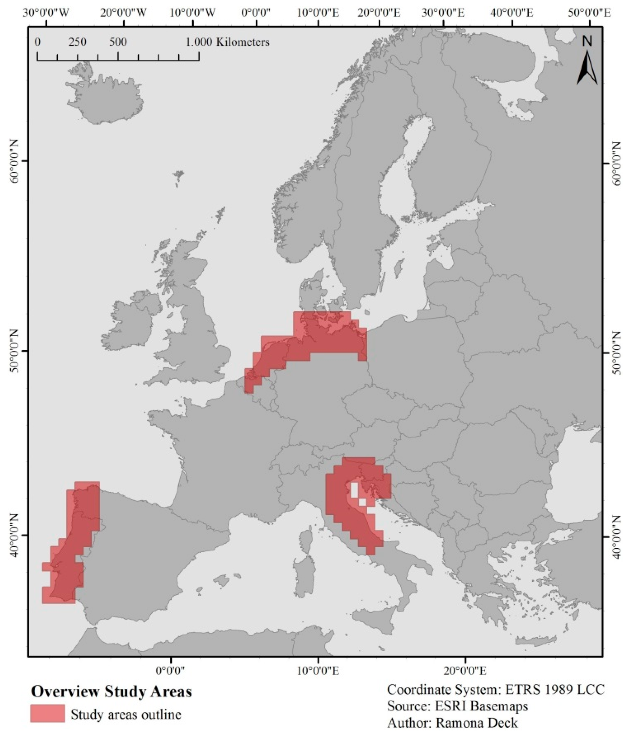
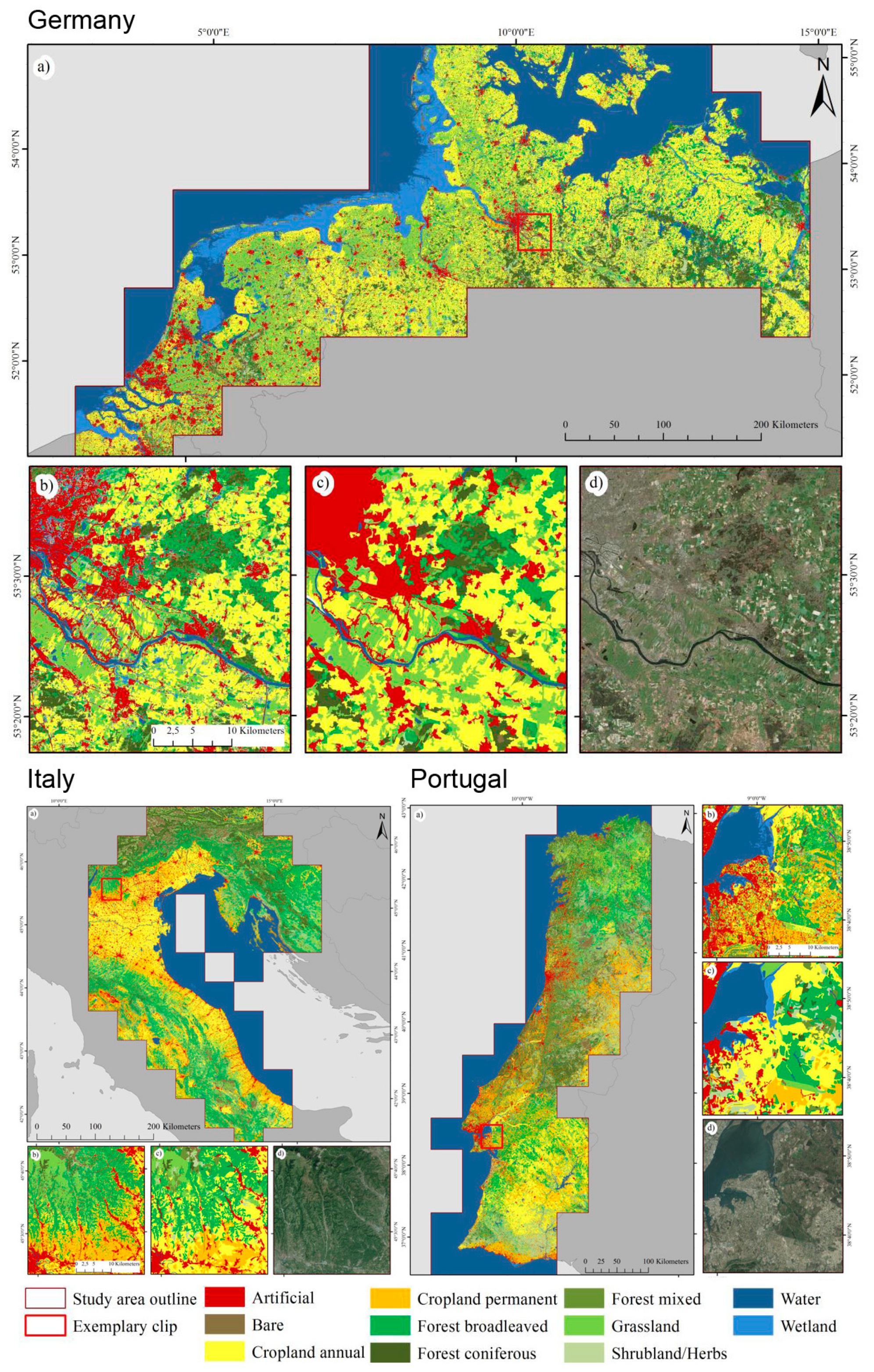
2.1. Study Area

In this study, three focus areas were selected (Figure 1). The northern study area (approximately 182,000 km2) is located at the North Sea and the Baltic Sea and covers the coastal zone of Germany, the Netherlands, and partly Belgium as well as Denmark. For simplification, this study area is hereinafter referred to as ‘Germany’. Facing the Atlantic Ocean, the second study area (approximately 150,000 km2), ‘Portugal’, covers almost the entire territory of Portugal and the autonomous community of Galicia in Spain. The third study area (approximately 156,000 km2), ‘Italy’, is composed of coastal zones located in the Mediterranean Sea, in particular the Adriatic Sea. The largest part is represented by a section of the eastern coastal zone of Italy, but also parts of Slovenia, Croatia, and Austria are involved. The selection of these three study areas is motivated by preferably diverse characteristics of the study regions to test the potential of the LU/LC classification in different coastal landscapes and climates.

2.2. Data Basis

2.2.1. Satellite Data

For this study, we acquired all Level 1 (L1T) terrain-corrected Landsat 7 and Landsat 8 scenes with their associated enhanced thematic mapper plus (ETM+) sensor, operational land imager (OLI), and thermal infrared sensor (TIRS) having not more than 60% cloud cover and an acquisition date between 1 December 2013 and 30 November 2014. In total, 511 scenes for Germany, 442 for Portugal, and 574 scenes for Italy met the criteria for a total of 30 Landsat WRS-2 path/rows intersecting the three study regions. In total 1527 Landsat scenes were acquired and stored on a local machine to be further processed with the TimeTools framework [10].
Furthermore, Shuttle Radar Topography Mission (SRTM) elevation data, available at a spatial resolution of 1 arc-second corresponding to approximately 30 m was acquired for the study regions [11].

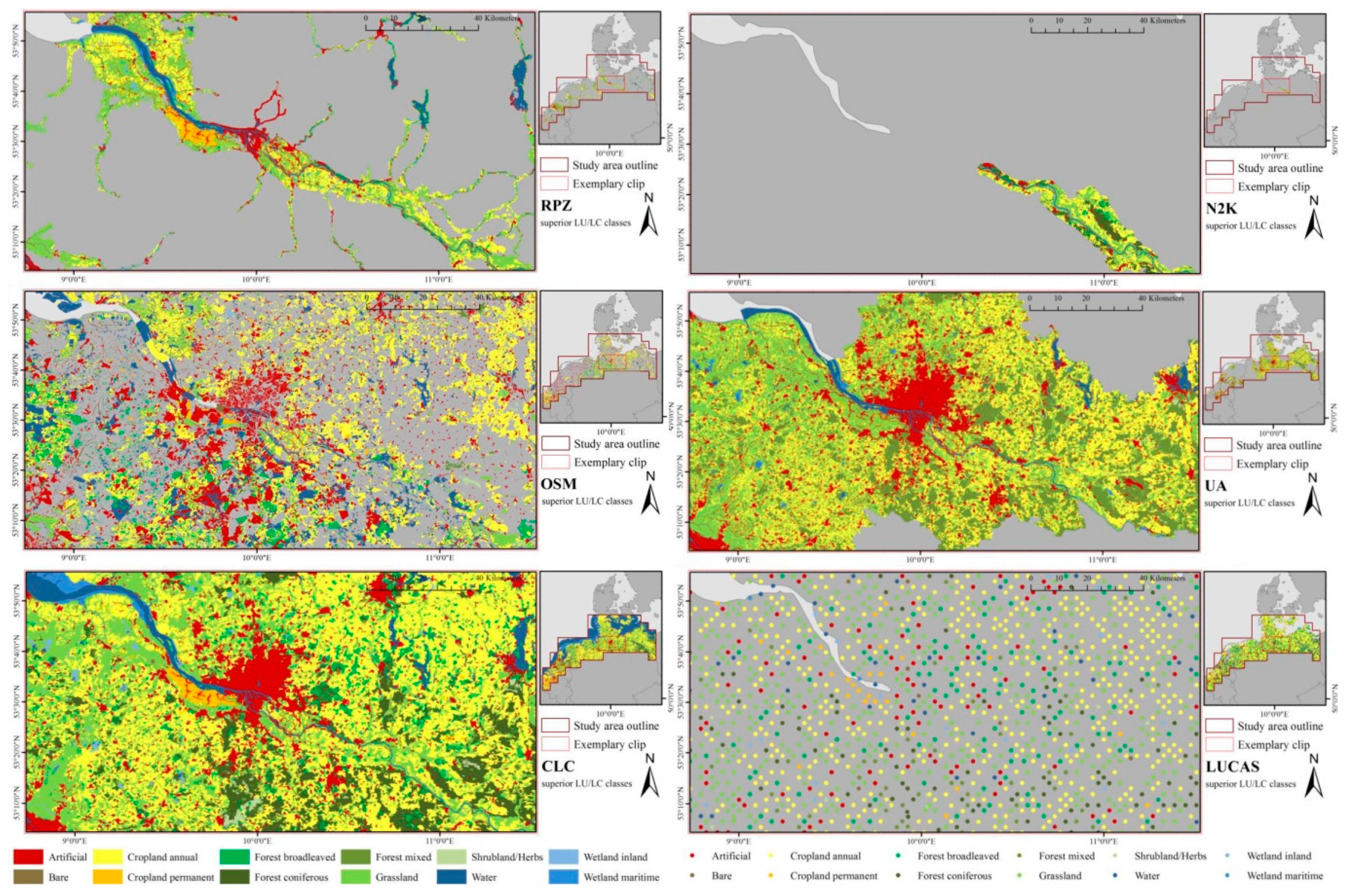
2.2.2. Land Use and Land Cover Data as Training and Reference Data Sets

Altogether, six different data sets were tested for collecting reference data with respect to pan-European applicability (Figure 2), which are briefly introduced in the following section:
  • The coordination of information on the environment (CORINE) program of the European Commission seeks to gather information on the state of the environment and is responsible for the coordination of this compilation within the Member States or likewise at an international level. This standardization ensures compatibility of data and results in a homogeneous pan-European wall-to-wall data set containing information about land cover and land use, hereinafter referred to as the CORINE Land Cover (CLC) data set. Initiated in 1985 and produced by the European Environment Agency, the program published its first inventory in 1990 [12,13]. Updates followed in the years 2000, 2006, and latest 2012, constantly extending the area covered, peaking in 39 involved EEA Member States and a total area of 5.8 million km2 [14]. Some parameters were kept unmodified in all CORINE land cover versions comprising the minimum mapping unit (MMU) of 25 hectares, the minimum mapping width (MMW) of 100 m for linear objects, and the working scale of 1:100,000 or the three-level land cover nomenclature containing a total of 44 individual classes. Later versions also take more recent satellite images into account and computer-assisted photo-interpretation as well as semiautomated approaches to reduce labor-intensive photo-interpretation. Apart from SPOT-4/5 data (2006), further optical and near infrared satellite images, such as Landsat-7’s ETM (2000), IRS P6’s sensor LISS III (2006 and 2012), and RapidEye (2012) were also used [12].
  • The Land Use and Coverage Area frame Survey (LUCAS) under the responsibility of EUROSTAT, the statistical office of the European Commission [15], is another European initiative related to land use and land cover inventory. LUCAS surveys are carried out every three years since 2006, and the latest published LUCAS survey dates from 2018 and comprises more than 330,000 collected sample points all over the 28 EU countries. The points are empirically registered in the field (in situ) and selected from a total of 1,100,000 points, distributed among the EU territory in a regular 2 km sampling grid. An MMU is not applicable. Instead, the surveyed point is defined as a circle with a radius of 1.5 m. Though, in specific cases, e.g., for nonhomogeneous classes, an extended observation area with a radius of 20 m around the actual point can be considered [16,17,18]. The classification system is subdivided into eight main land cover categories, comprising 84 subclasses and another 14 main categories describing land use, which are likewise segmented into 33 subcategories [13,15,19].
  • The Natura 2000 (NK2) data set only represents land cover and land use within selected Natura 2000 sites plus a surrounding buffer zone of 2 km and is therefore not a seamless wall-to-wall data set. The project was initiated by EEA and first published in 2006, an updated version was published for 2012 and covers 28 Member States. The underlying idea was to enhance support of biodiversity monitoring. N2K targets are habitats and zones valuable for endangered species and aims to stop the decline of these substantial areas. Customized to the needs of surveying and assessment of ecosystems and their services, an MMU of 0.5 ha and an MMW of 10 m is used. The four-level nomenclature consists of 62 classes and is based on main features of the already existing Mapping and Assessment of Ecosystems and their Services (MAES) typology combined with that of CLC. Especially level four meets the project specific requirements of N2K definitions. The total N2K area of interest aggregates to 160,444 km2. Along with very high resolution (VHR) SPOT-5 and SPOT-6 data, features of CLC, the European Urban Atlas (UA), Forest HRL, and additional reference and in situ data at country scale also serve as data for the classification [20].
  • Riparian Zones (RPZ) also provide LU/LC information for selected regions, thereby focusing on European rivers and adjacent buffer zones [17]. Riparian Zones are defined as the interface or transition zone between contiguous terrestrial and aquatic ecosystems, like rivers, streams, lakes, or even the sea [21]. Only rivers starting with a Strahler level of three are considered and buffer zones are adapted according to this level. The data set was also initiated by EEA and published in 2012 with a total coverage of approximately 525,000 km2 distributed in 39 Member States. An MMU of 0.5 ha and an MMW of 10 m is used, and accordingly the four-level nomenclature is referred to MAES and CORINE albeit containing 80 classes in this case. The main data sources are VHR SPOT-5 and SPOT-6 satellite data augmented by UA, HRL Imperviousness Degree and Tree Cover Density, CLC, Landsat-5/8, and N2K, amongst others.
  • The European Urban Atlas (UA) is a local data set of the Copernicus land monitoring services and is supported by the European Space Agency (ESA) and the European Environment Agency (EEA). As its name implies, LU/LC is tailored to the needs of urban areas, which can be very fragmented and therefore, an MMU of 0.25 ha for urban classes and 1 ha for non-urban classes is used. The data set is produced for major agglomerations, more precisely for so-called functional urban areas (FUA) and first published in 2006, followed by an updated version in 2012 with further updates planned in five-year cycles. The latest version covers 697 FUA, which includes most cities and their commuting zone exceeding 50,000 inhabitants in 28 Member States. The nomenclature is based on CORINE and GMES Urban Services. UA contains 28 classes in a four-level nomenclature, of which 17 are urban, while 11 are rural. The data mainly consists of VHR SPOT-5 satellite images combined with additional navigation data.
  • The OpenStreetMap (OSM) project started in 2004 in London and can be considered as a product of the development of today’s Web 2.0 that relies on a network of participating individuals that ties together the updating and exchanging of information [22]. Therefore, the integrity and coverage depends on the dedication of the people willing to map places and add information. User contribution is a core part of this crowdsourced project and given that anybody can edit OSM, rapid changes can be updated continuously. Hence, not only geographical trained persons, but rather amateurs can contribute to this patchwork project. With the collaboration of supporters, geographic information can be supplemented by ancillary information including names, cultural, or environmental information, which cannot be determined by remote sensing [23,24]. For completion of the maps, GPS tracks, satellite imagery, out-of-copyright maps, and aerial imagery was used. Aside from individual user participation, the import of already available public domain geographical information plays a major role [25].
Additionally, two more complementary LU/LC data sets were used as the basis for a comparative analysis with the derived products from this study:
  • Four Copernicus high resolution layers belonging to the pan-European section of the Copernicus program each providing information on a single LU/LC type, namely imperviousness (ranging 0–100%), forest (no forest, broadleaved, or coniferous forest), wetlands (binary), and permanent water bodies (binary). The wall-to-wall layers are generated at 20 m spatial resolution and cover 39 EEA Member States (5.8 million km2). The main data bases for the multispectral and object-oriented classification approach are multitemporal HR satellite imagery plus ancillary data available (e.g., vegetation indices, biophysical parameters) [26]. The maps are semi automatically produced in a collaborative initiative between the EEA, industry, and the EEA Member States.
  • GlobeLand30-2010 (GL30) is a seamless LU/LC data set with a global coverage at 30 m spatial resolution, developed mainly from Landsat and Chinese Huanjing-1 (HJ-1) satellite imagery. Ten major LU/LC classes are labeled, which are cultivated land, forest, grassland, shrubland, wetland, water bodies, tundra, artificial surfaces, bare land, and permanent snow and ice. Classification was implemented through pixel-based classification with subsequent object filtering to reduce the salt and pepper phenomenon [27,28].
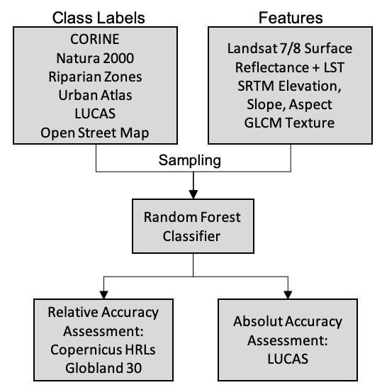
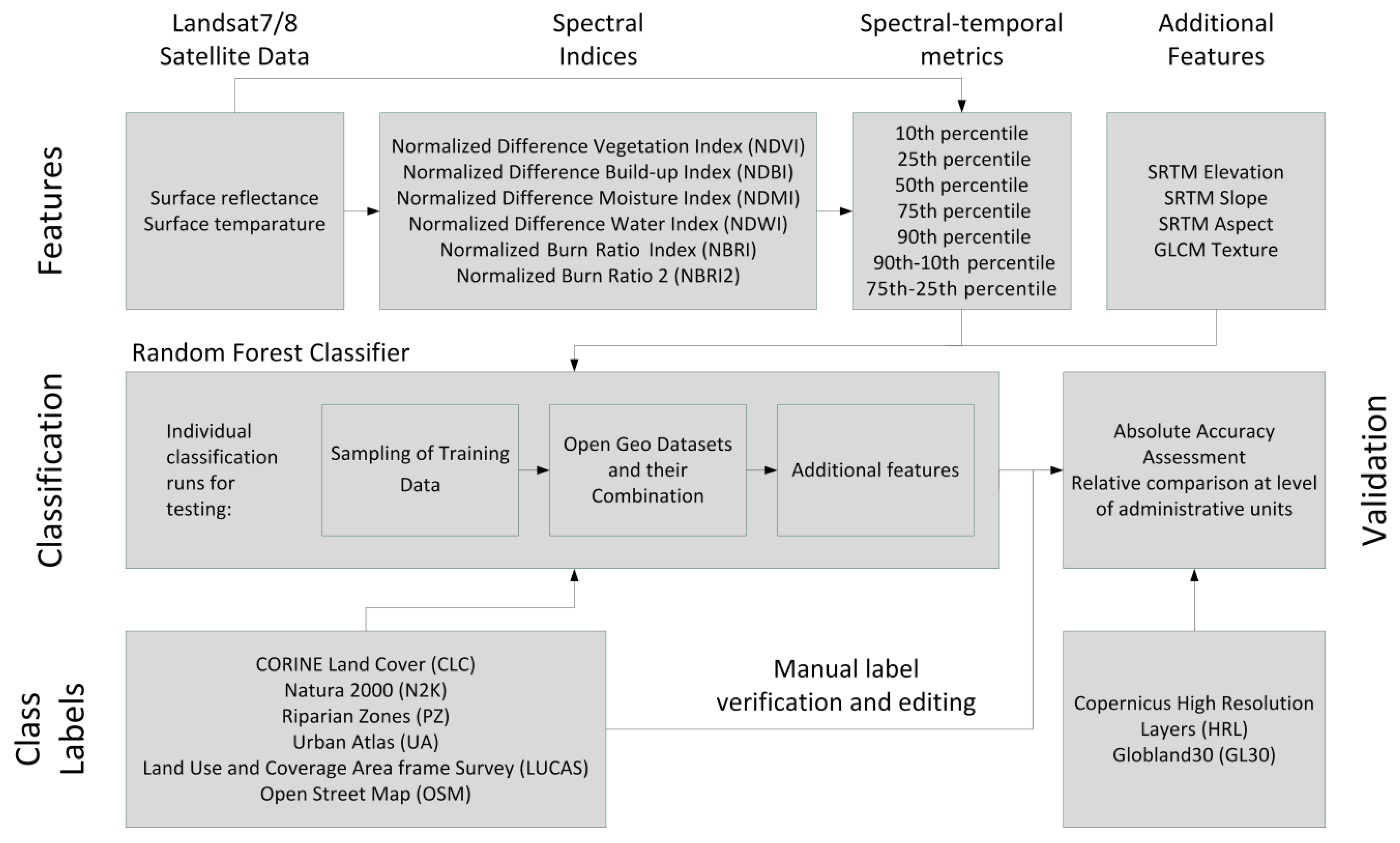
3. Methods

3.1. Preparation of Land Use and Land Cover Data Sets

The Copernicus data sets were downloaded from the Copernicus Land Monitoring website [29] in their latest versions, according to the respective pan-European or local categories. For all Copernicus data sets, the reference year is 2012, which can still be regarded as suitable for classification tasks based on satellite imagery ranging between 2013 and 2014. All products except the Copernicus HRLs were acquired in vector format. For RPZ, the data is partitioned in river catchments or regions. Fifteen of such regions were downloaded to cover the entire area of the study sites. The files for UA are separated in FUA, from which 59 were located at least partially in the study areas. Within OSM, every polygon feature is described by so-called tags that can be further specified by values. The user defined tags are grouped in several categories, from which only a selection was used in this study to keep the data volume manageable. The subset of tags used in this study includes land use, natural, water, and wetland, as they contain the required information to assign the polygons to their related class. OSM data required for the three study regions were downloaded for each country separately on 24 August 2016 in OSM-XML format from the Geofabrik website [30]. LUCAS data are only available as point data and were obtained from the Eurostat website [31]. The current version refers to the reference year of 2015 and hence, it represents the latest of all observed LU/LC data sets. Except for imperviousness, all HRLs were already available as 20 m binary maps. For imperviousness a proposed threshold of 30% was chosen to convert the density to a binary map (built-up/non-built-up) product [32]. GL30 is divided into 853 rectangular tiles, from which 11 were merged to a mosaic to cover the study areas. The data can be downloaded from the official website (http://glc30.tianditu.com/) and is available in raster format. All data sets were clipped to the study areas and were transformed to a consistent coordination system (ETRS-LCC).
A key challenge in terms of comparing different data sets is the variability evident in the nomenclature and definition of the diverse LU/LC classes. Therefore, harmonization of the different classification schemata is an inevitable requirement [33]. To support the matching of classes, currently existing comparisons of classification schemata were consulted and used as ancillary information. Batista e Silva et al. [34] combined CLC and UA in their study about a refined European LU/LC map and therefore, created a translation between these classifications. Estima and Painho [35] tried to find correspondence between CLC and OSM classes, while Büttner and Maucha [12] did the same for CLC and LUCAS in order to perform their accuracy assessment based on LUCAS. The six different classification systems of the data sets were compared and a selection of eleven classes was made, i.e., artificial, bare, cropland annual, cropland permanent, forest broadleaved, forest coniferous, forest mixed, shrubland/herbs, grassland, wetland, and water. A comprehensive overview of the grouping of subclasses of each data set can be seen in Appendix A. Only classes found in each of the six classification systems were considered. An exception is UA, for which no differentiation of the forest classes could be undertaken. Therefore, all forest polygons were assigned to forest mixed.
Classes with too heterogeneous features for the sensor applied, such as complex and heterogeneous agricultural areas, were omitted from the analysis. The same is true for classes that can only be labeled by knowing the respective land use, like sport and leisure facilities, urban green, or greenhouses. Furthermore, the classes glaciers and/or perpetual snow were regarded as irrelevant for our focus regions and hence, were also excluded. In the case of OSM, the OSM wiki was consulted to recognize the most important labels. A special entry in the wiki exists for values that are referring to respective CLC classes. This enhanced the matching of values and the classification scheme was further supplemented by values proposed by Estima and Painho [35]. Labels that were found in the OSM data, but not described in the wiki page were not included because of the uncertain definition.

3.2. Processing of Satellite Imagery

The well-known Fmask algorithm [36,37] was applied to all images to create cloud and cloud-shadow masks. The digital numbers of the downloaded scenes were converted to surface reflectance and surface temperature with ATCOR3 [38], which also includes a well-performing topographic correction procedure [39]. Based on the surface reflectance, we also computed the spectral indices, normalized difference vegetation index (NDVI), normalized difference buildup index (NDBI), normalized difference moisture index (NDMI), normalized difference water index (NDWI), the normalized burn ratio index (NBRI), and the normalized burn ratio 2 (NBR2). Finally, all layers were reprojected to the coordinate reference system ETRS89/ETRS-LCC and tiled into a uniform and regular grid of 50 km × 50 km for subsequent per pixel-based intra-annual time series processing. From all clear (cloud/cloud-shadow free) observations, we derived spatially contiguous spectral–temporal metrics at pixel level [10,40,41,42,43,44]. Therefore, for each 50 km × 50 km tile, multitemporal data stacks are generated for each of the six reflectance and thermal bands, as well as for the six spectral indices using all available satellite data. Subsequently, for each pixel individually, all clear observations within the stack were selected, ordered, and the 10th, 25th, 50th, 75th, and 90th percentiles were calculated and stored as new synthesized input features for the classification process. From the 10th and 90th percentiles and the 25th and 75th percentiles the differences were calculated, respectively, to have additional features robustly describing the intra-annual range between lowest and highest values within the temporal stack. The usage of such spectral–temporal metrics not only solves the problem of data gabs related to clouds, but also allows exploiting specific temporal patterns in the data that can be attributed, for example, to seasonal vegetation dynamics or different land use types. All processing steps described above were done in a fully automated manner using the TimeTools framework [10].

3.3. Classification

Land cover information was derived based on training data collected from the above-mentioned data sets. All classification tests were based on a random forest classifier under standard parameterization of 500 trees, which is the standard classifier implemented in the TimeTools framework [10]. The accuracy of derived results were evaluated under different classification scenarios, sampling strategies and training data distributions, different geodata sets and their various combinations, as well as different feature combinations for three different study areas. Thereby an efficient pathway was followed throughout the large variety of tests, by considering only the most promising configuration within one step as basis for the subsequent step.
As can be seen from Figure 3, a first assessment was examined to identify the prioritized method of collecting training samples combined with varying buffer sizes (Section 3.3.1). Based on the best performing sampling approach, the individual LU/LC data sets and their combination were evaluated as a training data base in automated classification procedures (Section 3.3.2), followed by the testing of additional input features (Section 3.3.3). Furthermore, a final classification test was performed through modification of the classification scheme in the course of a comparative analysis with two similar existing data sets for Europe (Section 3.5), based on zonal statistics on administrative boundaries as well as a verification of these two data sets with the reference data set created in the present study.

3.3.1. Sampling of Training Data

The first step in this analysis was to evaluate different ways of collecting training data. Three different methods of training point sampling from the existing land cover data sets were combined with two different buffer sizes applied to the underlying LULC data sets to avoid mixed pixels. The centroid method selects the representative geometric center of each LULC polygon as sample point. For irregular shaped polygons, it was ensured that the sample point always lies within the respective polygon. The grid method selects sample points according to a regular grid over the entire study area, regardless of prevailing land cover patterns. Following the guidelines for the LUCAS data set, a grid with the cell size of 2 km × 2 km was generated with a sample point placed in the center of each cell. The third method is a combination of the two aforementioned methods: In addition to the sampling points of the grid method, samples were added for polygons that do not contain a sampling point by applying the centroid method. The three different sampling schemes were applied to two rather contrasting data sets in terms of total polygon numbers and polygon sizes, i.e., the OSM and CLC data set. In addition, before sampling, for each polygon in the datasets two different buffer sizes were applied, i.e., 50 and 100 m beginning from the border of each polygon to the in side of the feature. Applying such a negative buffer erodes the polygons, which results in the minimization of edge effects, where mixed pixels are likely to occur and which may have negative effects on classification accuracy [45]. In total, 12 classifications (three sampling methods, two buffer sizes, two data sets) were performed for each study region on the basis of the temporal metrics (percentiles and differences of the percentiles) as input features.

3.3.2. Data Sets for Training Data Generation and Their Combination

The best sampling method from Section 3.3.1 was then applied to the remaining datasets, i.e., N2K, RPZ, UA, and LUCAS. Furthermore, the combination of all datasets and a combination of all datasets with wall-to-wall coverage (i.e., LUCAS, CLC, and OSM) was examined. By examining the different training data sets it was evident, however, that the distribution of samples among the specific classes in each dataset was considerably imbalanced, which can lead to heavy over or under estimations of certain classes [46,47]. Therefore, two more training data sets were generated using the CLC data set to observe the effect of imbalanced sample distributions. For the “median sample data set” (CLC-M) the number of samples for each class was reduced through randomly deleting samples until the median over all classes was reached. In this way, majority classes were down sampled [48]. However, since there are still classes that include fewer samples than the median, this method did not lead to a strict equal distribution. For the second training data set, the so called “combined median sample data set” (CLC-MC), additional samples for classes with fewer samples than the median over all classes were added by randomly selecting training points from the remaining data sets until the median number was reached. This led to a dataset with an equal number of training data for each class within each study region.

3.3.3. Inclusion of Additional Input Features

Finally, the best performing training data set from Section 3.3.2 was modified to include additional input features. For each study region, three training data sets were generated that supplemented the spectral–temporal metrics by a) topographic input features (elevation, slope, and aspect calculated from SRTM DEM), b) texture metrics based on the percentile features of the NDVI, and c) both topographic and texture features. The GLCM texture metrics were calculated according to Lu and Batistella [49] and comprised contrast, correlation, dissimilarity, entropy, mean, angular second moment, and variance in a 3 × 3 pixel neighborhood.

3.4. Accuracy Assessment

Validation of classification results were primarily done on the basis of a subset of LUCAS data which was left out from the LUCAS training process. The collection of the test data was carried out according to the following protocol of a random stratification procedure, which was already applied in Mack et al. [10]. First, we randomly shuffled the LUCAS points of each class. Second, according to the random order, we sequentially checked the points until 100 points valid for the testing purpose were identified. A point was considered valid if it was located in the centre pixel of a homogeneous 3 × 3 pixel neighborhood. A point was adjusted and also considered valid if it could be moved into a homogeneous neighborhood. However, a point was not moved out of its original class patch or further away than 300 m. We used Google Earth imagery for controlling the test samples. For classes, where 100 test points could not be reached, the lacking test data were randomly collected from the remaining five training data sets (CLC, N2K, RPZ, UA, and OSM) by applying the same verification process as before. For each class and study area, 100 test samples were collected according to this procedure, resulting in a total of 1200 samples collected for each study area, which sums up to 3600 data points altogether. A confusion matrix was calculated and the standard measures of classification accuracy, i.e., overall accuracy, producer’s (PAc) and user’s accuracies (UAc), and kappa coefficient, were derived from the matrix. Furthermore, the f1-score [50] as the harmonic mean of UAc and PAc was calculated. The range of the f1-score varies between 0 and 1, with 1 indicating the most accurate results [51].

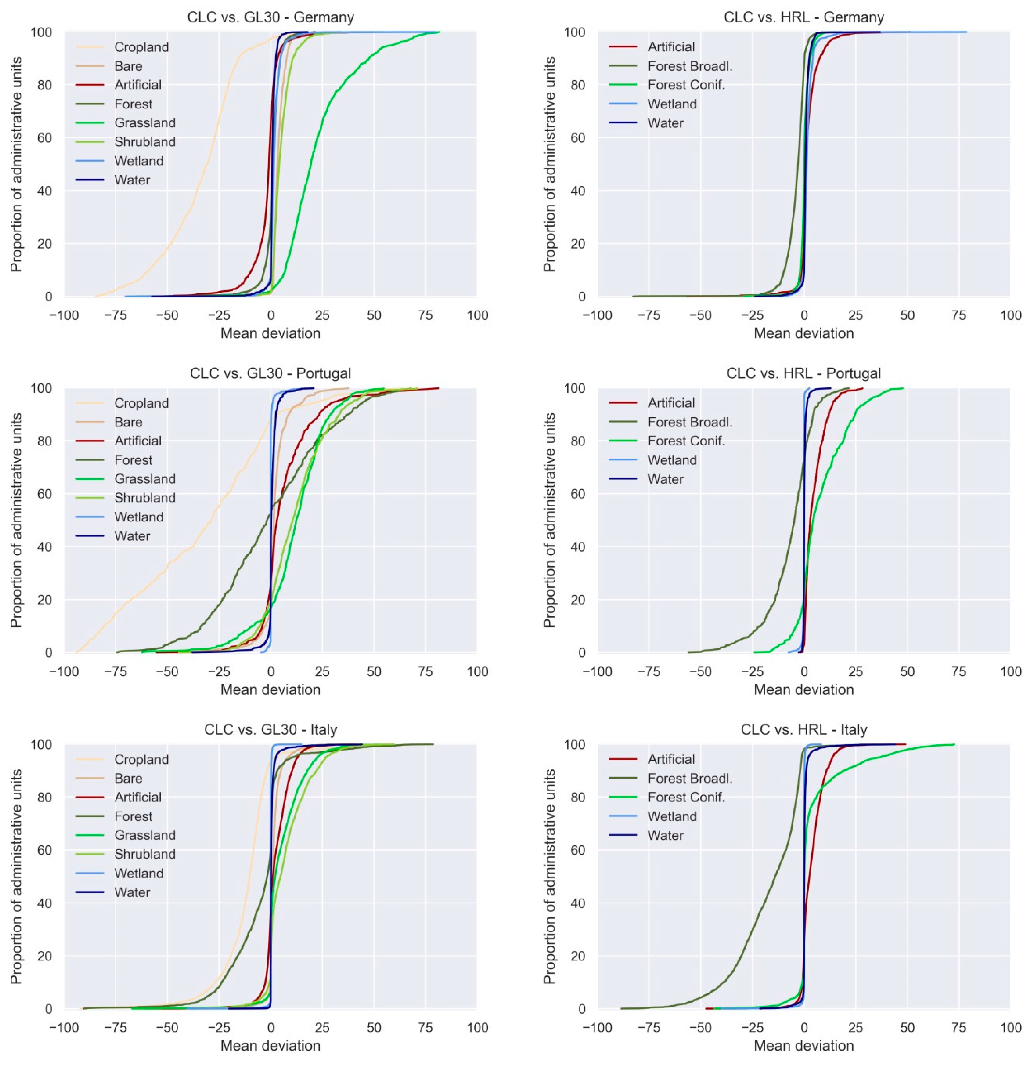
3.5. Comparison with Similar pan-European Open Land Cover Products

In addition to an absolute accuracy assessment, intuition was gained on the performance of our fully automated approach relative to existing manually edited products. Therefore, the classification output of the best performing combination from Chapter 3.3 was compared to two of the most commonly used, openly available land cover data sets for Europe with comparable spatial resolution, i.e., GL30 and the Copernicus HRLs. Therefore, two additional classifications were generated that matched the classes of these data sets.
For GL30 only eight classes were considered, although the data set includes initially ten classes. Two classes, namely Tundra and Permanent snow and ice, were excluded, since none of these classes were considered in the classification scheme of this study. Furthermore, in our training data the subcategories Forest broadleaved, Forest coniferous, and Forest mixed, as well as the two subcategories Cropland annual and Cropland permanent within the classification scheme of this study were merged to Forest and Cropland, respectively, to fit the scheme of GL30. Furthermore, with respect to the HRLs, a classification was performed with a modified classification scheme, where the subcategory Forest mixed was discarded from the training data to fit the classification scheme of the respective forest HRL. Accuracy of the GL30 and HRLs products were verified based on the data set and procedure described in Section 3.4. In addition, a quantitative comparison of relative land cover proportions was performed at administrative units [52] for each focus region.

4. Results

4.1. Sampling of Training Data

As can be seen from Table 1, the use of a 100 m buffer instead of a 50 m buffer leads to a significant reduction in samples for the training procedure. Averaged over the study regions, for CLC the reduction is about 13% and 16% in the case of the centroid method and the grid method, respectively. An even greater reduction in samples can be noticed for the OSM data set, due to its commonly smaller polygon sizes compared to CLC. The effects of the buffer account for a reduction of around 35% and 70% in the case of the grid method and centroid method, respectively. In general, the differences in f1-score among the different scenarios are neglectable, but in the majority of cases the 50 m buffer results in a better performance, and the same general pattern is evident over all study regions. Only for the OSM data set are the differences higher, ranging between 1% and 8%. When looking at the class specific performance, the effects of the larger buffer size become more evident. Particularly rare classes or classes with small patch sizes such as artificial and bare, lose a considerable number of training samples, which results in a significant reduction in accuracy of up to 7% for Germany, 13% for Portugal, or even 36% for Italy.
The respective sampling method applied also has significant effects on the total number of training instances and the sample distribution among the classes within each training data set. The centroid method results in more training samples than the 2 km grid method. The surplus is dependent on the landscape structure and samples can differ widely. With the largest average patch size of 3.75 km2 for CLC, the landscape is less fragmented in Germany, resulting in about equal amounts of samples for the grid and centroid method. The effect of the sampling method on total sample size is largest for the OSM dataset. The total number of samples resulting from the grid method makes up only about 2% of the sample size produced with the centroid method. In view of this, the difference in sample size between the combined grid–centroid training data and the centroid training data turned out to be relatively small, particularly for OSM.
With respect to the among-class homogeneity, a more homogeneous distribution can be observed for the centroid method compared to the grid method, as the former includes more samples for classes with small polygon sizes or for classes with typically fragmented distributions. As a result, rare classes or classes with small patch sizes are overrepresented, while the grid method provides a representative distribution of training samples. With respect to accuracy levels, the centroid method shows the highest f1-scores in nearly all cases. For CLC, the centroid method results in an increase in OA of 17% for the 50 m buffer and 20% for the 100 m buffer compared to the grid method. For OSM, the increase in OA amounts to 25% (50 m buffer) and 19% (100 m buffer), respectively, when applying the centroid method compared to the grid method. Despite the higher numbers of samples for classes with larger polygons in CLC, the f1-score for these classes are still lower compared to those of the centroid method, whereas classes with smaller polygons show higher f1-scores for the centroid method. The combined method results in no distinct improvement compared to the centroid method alone. On average, the difference in f1-score for the 50 m buffer varies only by 0.03 for Germany, by 0.04 for Italy, and 0.01 for Portugal, thereby showing no clear trend towards better performance for one single method.

4.2. Data Sets for Training Data Generation and Their Combination

The centroid sampling method applied with a 50 m buffer to each polygon, results in highly differing total numbers of training samples for each LU/LC data set. For Germany, for instance, training samples range from more than 330,000 for the UA data set to about 2100 samples for the N2K data set. This disparity depends on the total number of polygons and the spatial coverage of each data set. N2K and LUCAS generally show the lowest number of samples while UA, OSM, and RPZ have for all study areas the largest number of samples.
Furthermore, the distribution of samples per class is rather heterogeneous. Certain land cover types are prominently represented in the data sets, while others are scarce and hold a very limited number of samples. Grassland and cropland annual are the most dominant classes within the training data set for Germany, while for Portugal, shrubland/herbs causes an imbalance due to its large coverage. In Italy, shrubland/herbs, grassland, and forest broadleaved are the best represented classes in the training data set. For Germany, CLC is the data set with the most homogeneous distribution. For Portugal, the RPZ data set shows the most even distribution among all data sets. For Italy, CLC is the most balanced data set. The modified CLC data set CLC-M shows a far more homogeneous distribution with maximum samples of 2222 for Germany, 3429 for Portugal and 2827 for Italy. These numbers represent the specific median over all classes in the study regions.
With respect to the achieved accuracy levels (Table 2), the CLC and RPZ data sets perform with averaged OA of 61% and 57% best, while OSM and LUCAS performed worst only achieving OAs of around 48% averaged over all study regions. In general, data sets with a more homogeneous spatial distribution and more balanced sample distribution among the classes performed better in the classification. Furthermore, Italy, showing the most balanced distribution of samples among the classes, achieved the best results in all data sets, except for OSM.
With respect to the sample imbalance in the training data, specific patterns of confusion in the results can be observed. For Germany, grassland is the most frequent class and; therefore, high errors of commission emerge on costs of shrubland/herbs, cropland permanent, and wetland, which are scarcely represented in the sample distribution. Cropland permanent is not even classified at all in four out of six data sets, due to its high confusion with cropland annual and grassland and therefore, high errors of omission occur. Artificial also ranks among the more prominent classes in most of the data sets, which causes errors of omission especially for bare. Portugal shows similar patterns with high error of commission for the dominant shrubland/herbs class on costs of wetland, bare, cropland permanent, and partially the forest classes, which belong to the less dominant classes. In Italy, the more balanced distribution is accompanied by less confusion among classes, resulting in higher accuracy levels. However, grassland is confused especially with shrubland/herbs and wetland, which causes error of omission for the underrepresented classes. Forest broadleaved also counts to the more frequent classes, which is expressed by high errors of commission on the expense of shrubland/herbs.
The combination of the different LU/LC data sets (CLC-ext, ALL) had no positive effects on accuracy levels when compared to the best performing individual data set (CLC) for the study areas of Germany and Italy. However, the case is different for Portugal. Here the different combinations performed better than the individual data sets, although the improvements were, at about 1–3%, not large. Remarkable improvements, however, were evident for the modified CLC data sets, i.e., CLC-M and CLC-MC. With respect to accuracy levels, a significant improvement in OA of 5% for Portugal and even 10% for Germany can be observed when cutting down the samples to the median (CLC-M). No appreciable change in accuracy levels can be recognized for Italy, which already showed a rather homogeneous sample distribution among the classes. The reduction of samples for the dominant classes resulted in a particularly large performance increase for the rare classes. This was clearly evident for Germany for the classes cropland permanent, shrubland/herbs, or bare, and for Portugal for the classes artificial and grassland. Adding further samples in the training data for rare classes, as done for the combined median sample data set (CLC-MC), even further improved the results compared to the median sample data set. With an increase of 0.42, the largest class specific improvement can be seen for cropland permanent after adding additional samples. Less grassland is mistakenly labeled as cropland permanent, which also yields in a better f1-score for grassland.

4.3. Inclusion of Additional Input Features

The use of additional features in the classification process led to further improvements, although these were relatively minor (Table 3). By adding only additional topography or texture metrics, the increase accounts for around 2% and 1%, respectively, averaged over all study regions. The best result was obtained by using all input features, which had the highest impact for Italy with an improvement of about 4% in OA. When looking at the individual classes, no outstanding pattern or relationship with respect to accuracy improvement could be observed.
The final map product of the classification performing best, i.e., the CLC combined median sample data set with a 50 m buffer applied based on the centroid method for sampling collection together with all 119 available input parameters, can be seen in Figure 4 for the three study regions. The general similarities to the initial CLC data set (c) are clearly evident. However, the map product of this study (a) is characterized by a higher resolution; therefore, more details become visible.

4.4. Comparison with Open Land Cover Products

Table 4 gives the overall accuracies for the classification based on the CLC modified median sample data set with an adapted classification scheme to fit to the GL30 and HRL products. Due to the reduced number of classes, the derived product achieves an averaged OA of about 75% over all study areas, while the GL30 product has about a 14% lower OA over all study areas. Particularly for the classes bare, grassland, and shrubland/herbs, a considerably lower f1-score of 42% can be observed for GL30, averaged over these classes and study areas. The comparison with the HRLs led to no clear trend with respect to superiority of one product over all study areas. For Germany and Italy, slightly higher results could be achieved by the product of this study, while for Italy, the HRL layers performed better.
Figure 5 shows the differences in relative land cover proportions between our product and the GL30 and the HRL products, respectively, calculated on district level for all three study regions. Due to the larger deviations in absolute accuracy levels for GL30 compared to the HRLs, differences in relative proportions are also higher for the GL30 product. However, the comparison still reveals that for most classes differences are rather low. Particularly for the classes artificial, bare, wetlands, and water, the majority of districts, i.e., on average 69%, 75%, 96%, and 97%, respectively, show deviations below 5%. In Italy and Portugal, the GL30 product shows high confusion of shrubland/herbs with the forest and cropland classes, resulting in around half and one third of all districts lying below 5% difference. Due to the strong overestimation of cropland and underestimation of grassland in the GL30 product, these classes are at the lower end, resulting in large differences over all study regions with an average of only 11% and 26% of districts below the 5% threshold. Differences between the HRL products and the automatically derived classification are much smaller compared to the GL30 product. For Germany, proportions of wetland, water, forest broadleaved, and forest coniferous vary below 5% for more than 90% of districts. For Portugal and Italy, the differences for the forest classes are more pronounced. Here, the HRLs show higher proportions of forest broadleaved and smaller proportions of forest coniferous. On average, two thirds of districts in Italy and Portugal are below the 5% threshold. The artificial class also shows relatively high concordance below 5% deviation for two thirds of units for Germany and Portugal. Only for Italy are the differences higher, resulting in only about one third of districts below 5% deviation.

5. Discussion

In this study, a specific challenge was the harmonization of the LU/LC classification schemes of the different data sets used. This has always been a challenging task, as different definitions and class labels are used among the data sets and usually no standardized translation keys exist. Matching classes is particular difficult in the case of OSM, as only uncertain descriptions are available in the OSM wiki, a comprehensive overview of classes is lacking. Furthermore, tags are user-defined often made by ‘nonspecialists’ without knowledge of common standards and thus are strongly heterogeneous. [35,53,54,55,56]. Similar sources of uncertainty may occur for a number of Copernicus data sets. A common approach in generating these data sets is manual digitization of satellite imagery, which is also a source of error in delineating the correct geometry and choosing the appropriate label, as interpretation mistakes can occur. Another element of uncertainty is not only the subjectivity of individual contributors, but also the differences of interpretation and classification on a country-scale. The data sets generated within the framework of the Copernicus project are predominantly compilations of single data sets from the respective countries. Despite the existence of standard methods and interpretation rules in technical guides, there is no guarantee of complete consistency among the products of the countries, which may negatively influence the accuracy [34,57].
Further emphasis was made in the analysis of different methods of training sample collection to investigate their influence on the overall map accuracy. Regarding the different sampling methods, the choice of the buffer width has a clear effect on the accuracy. Negative buffers to erode polygons were also applied in other studies [45,58,59]. The size of the buffer had a particular strong effect on the grid sampling, because in this approach samples are distributed systematically over the study area without regard to the landscape structure. Therefore, the possibility of a sample lying close to borders of polygons is higher than for centroid samples, which are placed in the center of the polygons for minimizing edge effects. In the case of the 100 m buffer, the assumed edge effects through mixed pixels are already minimized by the smaller buffer and thus, applying a larger buffer implicates no significant increases in f1-score of the specific classes. Instead, reducing the number of samples through application of the 100 m buffer, results in lower accuracies, which might be explained by the resulting underrepresentation of samples for smaller polygons in the training data.
However, applying buffers around polygons or selecting the center point of a polygon is not a guarantee for avoiding mixed pixels or even for preventing the assignment of erroneous land cover labels. For the CLC data set, smaller units than the minimum mapping unit of 25 ha are assigned to adjacent polygons of the dominant LU/LC class around the patch, which can result in heterogeneous polygons [60]. The same applies to the finer but still generalized polygons of the other data sets, such as OSM [61]. In view of this, further research has to focus on the development of indicators, for example based on texture metrics or segmentation approaches, to characterize homogeneity of class patches [10]. With respect to the LUCAS data set, the challenge related to scale differences between satellite sensor and geodata basis for sampling is of contrasting nature compared to CLC. The label of a LUCAS point represents the respective LU/LC within a radius of 1.5 m and within an extended radius of 20 m for heterogeneous classes, which is much smaller than a 30 m Landsat pixel [34]. In order to exclude samples that are more likely to be located in a heterogeneous and fragmented environment resulting in mixed training pixels, the exploitation of the abundant LUCAS metadata may be an option, such as applied in Mack et al. [10], who filtered sample points according to patch homogeneous information extracted from the metadata.
The results clearly demonstrate that it is not the total number of samples alone that is important for achieving promising accuracy levels. Particularly, the distribution of samples among the classes is of central relevance, as also documented in previous studies [46,47]. This was evident already in the sampling. Accuracy was highest for the centroid method in nearly all cases. The latter converged the number of samples between dominant and rare classes, whereas the grid method, resulting in a more representative sample distribution for the study area, performed significantly worse in every study region, each buffer scenario, and for both OSM and CLC. Furthermore, the blind combination of all data sets without considering the among-class homogeneity in the sample distribution did not lead to considerable improvements compared to using the individual data sets alone. Increasing the training instances of the less frequent classes by selectively combining samples from the individual data sets and down sampling samples for dominant classes led to both a better performance of less represented classes and higher accuracies of the prevalent LU/LC classes. The impact of imbalanced training data and respective effects of over and under sampling were also investigated in other studies [59,62]. They found that the effects of resampling increased, the more distinctive the degree of class imbalance was, the more complex the landscape and the smaller the number of training samples. Other methods to consider include giving less frequent classes a higher weight, neglecting only noisy samples of the majority classes, or sampling more points for the minority class by replication [46]. SMOTE (Synthetic Minority Oversampling Technique) for instance, is a technique that downsamples majority class samples and adds minority class samples by interpolating pairs of closest neighbors [63,64].

6. Conclusions

The results of this study provide new insights into the applicability of openly available pan-European geodata for automated LU/LC information retrieval. In total, 1527 Landsat-7 and Landsat-8 scenes ranging from December 2013 to November 2014, as well as SRTM elevation data were acquired for three coastal focus regions in Europe, to generate a total of 119 input features, which were evaluated in combination with six LU/LC data sets for training data generation. Furthermore, several scenarios were tested in order to obtain optimal results with respect to the various aspects in the LU/LC generation process. These aspects include spatial sampling strategies, class homogeneity of training data based on different data sets and their combination, as well as the effects of additional features, such as topography and texture metrics. With successive modifications of the training sample set, the final scenario for the same number of classes improved the result by 11%, on average, with the highest values obtained between 60% and 72%.
With these accuracy levels, the fully automated method, based on existing European LU/LC data sets as the training data base in combination with high-resolution and multitemporal Landsat satellite imagery, showed high potential for deriving dominant LU/LC information for large scales with minimum manual effort. The approach might not reach quality levels of tailor-made local maps generated through laborious manual classification approaches, but its advantage lies in the possibility of a simple and fast generation of LU/LC information for a given region in Europe; therefore, being a time- and cost-saving approach. In view of this, the results of this study could facilitate the development of a Copernicus service for on-demand LU/LC retrieval, complementing the official pan-European Land Services, particularly during their multiannual product cycles.
The study showed that factors such as total amount of samples, spatial coverage for training data, and the distribution of samples among the classes were crucial for achieving satisfactory accuracy levels. Data sets such as RPZ, UA, or N2K do not provide a wall-to-wall coverage and resulted in rather imbalanced training data distributions. Therefore, these data sets showed generally not the best classification performance. Additionally, the LUCAS data set generated through a systematic sampling scheme showed to have a strong inhomogeneity with respect to the among-class distribution. Furthermore, training data sets based on LUCAS resulted in the smallest number of samples compared with the other data sets, thus generally resulting in accuracy levels at the lower end. The CLC data set resulted in the highest accuracy levels in most cases. Linked to the good performance might be the wall-to-wall coverage of this data set and the least inhomogeneous distribution of samples throughout the various landscapes of the study areas.
The sole combination of entire training data sets, with the aim to improve spatial coverage or to increase the number of total samples, did not lead to significant improvements in classification accuracy. However, the selective combination of samples from different data sets for specific classes targeted to increase homogeneity within the overall training data set, in most cases resulted in significant improvements in the classification results. Accuracy levels not only improved for those classes of which the number of samples increased, but also for the dominant classes, which lost relative weight within the training data set.
The comparison of the fully automated map generated in this study, with available comparable LU/LC products, shows the great potential of the proposed method. Particularly in contrast with GL30, the better performance of a regionally automatically generated map compared with the use of a global map for local or regional scale purposes is unambiguous. This is not surprising, considering the much more complex classification requirements on a global scale. The performance of the proposed method compared to HRLs is also remarkable. The layers are developed in large-scale initiatives and under extensive manual working efforts to provide a more detailed view on actual LU/LC patterns complementary to CLC. The automated method introduced in this study achieves comparable high levels of accuracy for most of the HRLs.

Author Contributions

Conceptualization, P.L. and B.M.; methodology, R.D., P.L. and B.M; validation, R.D.; formal analysis, R.D.; writing—original draft preparation, R.D. and P.L.; writing—review and editing, P.L., M.O. and J.H.; visualization, R.D. and P.L.

Funding

This research received no external funding.

Acknowledgments

Special thanks go to NASA and USGS for providing the Landsat data and download services for the data used in this study.

Conflicts of Interest

The authors declare no conflict of interest. The funders had no role in the design of the study; in the collection, analyses, or interpretation of data; in the writing of the manuscript, or in the decision to publish the results.

Appendix A

Harmonization of the classification schemata from the six data sets. Classes not included in the study are marked red* with an asterisk.

References

  1. Kuenzer, C.; Leinenkugel, P.; Vollmuth, M.; Dech, S. Comparing global land-cover products—Implications for geoscience applications: An investigation for the trans-boundary Mekong Basin. Int. J. Remote Sens. 2014, 35, 2752–2779. [Google Scholar] [CrossRef]
  2. Herold, M.; Woodstock, C.E.; Loveland, T.R.; Townshend, J.; Brady, M.; Steenmans, C.; Schmullius, C.C. Land-cover observations as part of a global earth observation system of systems (GEOSS): Progress, activities, and prospects. IEEE Syst. J. 2008, 2, 414–423. [Google Scholar] [CrossRef]
  3. Global Earth Observation System of Systems GEOSS: 10-Year Implementation Plan Reference Document. 2005. Available online: http://earthobservations.org/documents/10-Year%20Implementation%20Plan.pdf (accessed on 24 June 2018).
  4. Lamine, S.; Petropoulos, G.P.; Kumar Singh, S.; Szabó, S.; Bachari, N.; Srivastava, P.K.; Suman, S. Quantifying Land Use/Land Cover Spatio-Temporal Landscape Pattern Dynamics From Hyperion Using SVMs Classifier and FRAGSTATS®. Geocarto Int. 2017, 1–47. [Google Scholar] [CrossRef]
  5. Breger, P.; Malacarne, M.; Podaire, A.; Campbell, G.; Doherty, M.; Bruzzi, S. Global Monitoring for Environment and Security (GMES): The Services Establishing an Initial GMES Capacity. In Proceedings of the 31st International Symposium on Remote Sensing of Environment, Saint Petersburg, Russia, 20–24 June 2005. [Google Scholar]
  6. Pérez-Hoyos, A.; García-Haro, F.J.; San-Miguel-Ayanz, J. Conventional and fuzzy comparisons of large scale land cover products: Application to CORINE, GLC2000, MODIS and GlobCover in Europe. ISPRS J. Photogramm. Remote Sens. 2012, 74, 185–201. [Google Scholar] [CrossRef]
  7. Rogan, J.; Chen, D. Remote sensing technology for mapping and monitoring land-cover and land-use change. Prog. Plan. 2004, 61, 301–325. [Google Scholar] [CrossRef]
  8. Lee, C.; Gasster, S.D.; Plaza, A.; Chang, C.-I.; Huang, B. Recent Developments in High Performance Computing for Remote Sensing: A Review. IEEE J. Sel. Top. Appl. Earth Obs. Remote Sens. 2011, 4, 508–527. [Google Scholar] [CrossRef]
  9. Cihlar, J. Land cover mapping of large areas from satellites: Status and research priorities. Int. J. Remote Sens. 2000, 21, 1093–1114. [Google Scholar] [CrossRef]
  10. Mack, B.; Leinenkugel, P.; Kuenzer, C.; Dech, S. A semi-automated approach for the generation of a new land use and land cover product for Germany based on Landsat time-series and Lucas in-situ data. Remote Sens. Lett. 2017, 8, 244–253. [Google Scholar] [CrossRef]
  11. Kobrick, M. On the Toes of Gianst—How SRTM was Born. Photogramm. Eng. Remote Sens. 2006, 72, 206–210. [Google Scholar]
  12. European Environment Agency. The Thematic Accuracy of Corine Land Cover 2000—Assessment Using LUCAS; 2006; ISBN 978-92-9167-844-0. Available online: https://www.eea.europa.eu/publications/technical_report_2006_7 (accessed on 12 March 2018).
  13. Komp, K.-U. High Resolution Land Cover/Land Use Mapping of Large Areas Current Status and Upcoming Trends. Photogramm.-Fernerkund.-Geoinf. 2015, 2015, 395–410. [Google Scholar] [CrossRef]
  14. Manakos, I.; Braun, M. (Eds.) Land Use and Land Cover Mapping in Europe: Practices & Trends; Remote Sensing and Digital Image Processing; Springer: Dordrecht, The Netherlands, 2014; ISBN 978-94-007-7969-3. [Google Scholar]
  15. Eurostat LUCAS 2012 (Land Use/Cover Area Frame Survey), Technical Reference Document C3. 2013, p. 79. Available online: https://ec.europa.eu/eurostat/documents/205002/208012/LUCAS2012_C3-Classification_20131004_0.pdf (accessed on 11 June 2018).
  16. Eurostat LUCAS 2012 (Land Use/Cover Area Frame Survey), Technical Reference Document C1. 2013, p. 74. Available online: https://ec.europa.eu/eurostat/documents/205002/208012/LUCAS2012_C1-InstructionsRevised_20130110b.pdf/10f750e5-5ea0-4084-a0e7-2ca36c8f400c (accessed on 11 June 2018).
  17. Buck, O.; Haub, C.; Woditsch, S.; Lindemann, D.; Kleinewillinghöfer, L.; Hazeu, G.; Kosztra, B.; Kleeschulte, S.; Arnold, S.; Hölzl, M. Analysis of the LUCAS Nomenclature and Proposal for Adaptation of the Nomenclature in View of Its Use by the Copernicus Land Monitoring Services; European Environment Agency: Copenhagen, Denmark, 2015; p. 142. [Google Scholar]
  18. Martino, L.; Fritz, M. New Insight into land Cover and Land Use in Europe. Stat. Focus 2008, 33, 1–8. [Google Scholar]
  19. Eurostat LUCAS 2015 (Land Use/Cover Area Frame Survey), Technical Reference Document C3. 2015, p. 93. Available online: https://ec.europa.eu/eurostat/documents/205002/6786255/LUCAS2015-C3-Classification-20150227.pdf/969ca853-e325-48b3-9d59-7e86023b2b27 (accessed on 11 June 2018).
  20. European Environment Agency Copernicus Initial Operations 2011–2013–Land Monitoring Service Local Component: LC/LU Mapping of a Selection of Natura2000 (N2K) Sites; Natura2000 Product Specifications; European Environment Agency: Copenhagen, Denmark, 2015; p. 10.
  21. Naiman, R.J.; Decamps, H. The Ecology of Interfaces: Riparian Zones. Annu. Rev. Ecol. Syst. 1997, 28, 621–658. [Google Scholar] [CrossRef] [Green Version]
  22. O’Reilly, T. What Is Web 2.0: Design Patterns and Business Models for the Next Generation of Software; University Library of Munich: Munich, Germany, 2007. [Google Scholar]
  23. Goodchild, M.F. Citizens as Voluntary Sensors: Spatial Data Infrastrcuture in the World of Web 2.0. Int. J. Spat. Data Infrastruct. Res. 2007, 2, 24–32. [Google Scholar]
  24. Haklay, M. How Good is Volunteered Geographical Information? A Comparative Study of OpenStreetMap and Ordnance Survey Datasets. Environ. Plan. B Plan. Des. 2010, 37, 682–703. [Google Scholar] [CrossRef] [Green Version]
  25. Haklay, M.; Weber, P. OpenStreetMap: User-Generated Street Maps. IEEE Pervasive Comput. 2008, 7, 12–18. [Google Scholar] [CrossRef]
  26. Congedo, L.; Sallustio, L.; Munafò, M.; Ottaviano, M.; Tonti, D.; Marchetti, M. Copernicus high-resolution layers for land cover classification in Italy. J. Maps 2016, 12, 1195–1205. [Google Scholar] [CrossRef] [Green Version]
  27. National Geomatics Center of China (NGCC). 30-m Global Land Cover Dataset—GlobeLand30; NGCC: Bejing, China, 2014; p. 25. [Google Scholar]
  28. Ran, Y.; Li, X. First comprehensive fine-resolution global land cover map in the world from China—Comments on global land cover map at 30-m resolution. Sci. China Earth Sci. 2015, 58, 1677–1678. [Google Scholar] [CrossRef]
  29. Copernicus Copernicus Land Monitoring Service. Available online: https://land.copernicus.eu/ (accessed on 19 June 2018).
  30. Geofabrik GmbH Geofabrik Downloads—OpenStreetMap Data. Available online: http://download.geofabrik.de/ (accessed on 24 August 2016).
  31. Eurostat Eurostat Land Cover/Use Statistics (LUCAS). Available online: https://ec.europa.eu/eurostat/web/lucas/ (accessed on 29 March 2018).
  32. Maucha, G.; Büttner, G.; Kosztra, B. European Validation of GMES FTS Soil Sealing Enhancement Data. In Proceedings of the 32nd EARSeL Symposium, Remote Sensing and Geoinformation, Mikonos, Greece, 21–24 May 2011; pp. 223–238. [Google Scholar]
  33. Jansen, L.J.M. Harmonization of land use class sets to facilitate compatibility and comparability of data across space and time. J. Land Use Sci. 2006, 1, 127–156. [Google Scholar] [CrossRef]
  34. Batista e Silva, F.; Lavalle, C.; Koomen, E. A procedure to obtain a refined European land use/cover map. J. Land Use Sci. 2013, 8, 255–283. [Google Scholar] [CrossRef]
  35. Estima, J.; Painho, M. Exploratory Analysis of OpenStreetMap for Land Use Classification. In Proceedings of the Second ACM SIGSPATIAL International Workshop on Crowdsourced and Volunteered Geographic Information, Orlando, FL, USA, 5–8 November 2013; ACM: New York, NY, USA, 2013; pp. 39–46. [Google Scholar]
  36. Zhu, Z.; Woodcock, C.E. Object-based cloud and cloud shadow detection in Landsat imagery. Remote Sens. Environ. 2012, 118, 83–94. [Google Scholar] [CrossRef]
  37. Zhu, Z.; Wang, S.; Woodcock, C.E. Improvement and expansion of the Fmask algorithm: Cloud, cloud shadow, and snow detection for Landsats 4-7, 8, and Sentinel 2 images. Remote Sens. Environ. 2015, 159, 269–277. [Google Scholar] [CrossRef]
  38. Richter, R.; Schläpfer, D. Atmospheric/Topographic Correction for satellite Imagery, ATCOR-2/3 User Guide, version 6.3; DLR and ReSe Applications: Wessling, Germany; Wil, Switzerland, 2016; p. 263. [Google Scholar]
  39. Richter, R.; Kellenberger, T.; Kaufmann, H. Comparison of Topographic Correction Methods. Remote Sens. 2009, 1, 184–196. [Google Scholar] [CrossRef] [Green Version]
  40. Griffiths, P.; Müller, D.; Kuemmerle, T.; Hostert, P. Agricultural land change in the Carpathian ecoregion after the breakdown of socialism and expansion of the European Union. Environ. Res. Lett. 2013, 8, 045024. [Google Scholar] [CrossRef]
  41. Griffiths, P.; Kuemmerle, T.; Baumann, M.; Radeloff, V.C.; Abrudan, I.V.; Lieskovsky, J.; Munteanu, C.; Ostapowicz, K.; Hostert, P. Forest disturbances, forest recovery, and changes in forest types across the Carpathian ecoregion from 1985 to 2010 based on Landsat image composites. Remote Sens. Environ. 2014, 151, 72–88. [Google Scholar] [CrossRef]
  42. Hansen, M.; Potapov, P.; Margono, B.; Stehman, S.; Turubanova, S.; Tyukavina, A. Response to Comment on “High-resolution global maps of 21st-century forest cover change.”. Science 2014, 344, 981. [Google Scholar] [CrossRef]
  43. Müller, H.; Rufin, P.; Griffiths, P.; Barros Siqueira, A.J.; Hostert, P. Mining dense Landsat time series for separating cropland and pasture in a heterogeneous Brazilian savanna landscape. Remote Sens. Environ. 2015, 156, 490–499. [Google Scholar] [CrossRef] [Green Version]
  44. Rufin, P.; Müller, H.; Pflugmacher, D.; Hostert, P. Land use intensity trajectories on Amazonian pastures derived from Landsat time series. Int. J. Appl. Earth Obs. Geoinf. 2015, 41, 1–10. [Google Scholar] [CrossRef]
  45. Balzter, H.; Cole, B.; Thiel, C.; Schmullius, C. Mapping CORINE Land Cover from Sentinel-1A SAR and SRTM Digital Elevation Model Data using Random Forests. Remote Sens. 2015, 7, 14876–14898. [Google Scholar] [CrossRef] [Green Version]
  46. Mellor, A.; Boukir, S.; Haywood, A.; Jones, S. Exploring issues of training data imbalance and mislabelling on random forest performance for large area land cover classification using the ensemble margin. ISPRS J. Photogramm. Remote Sens. 2015, 105, 155–168. [Google Scholar] [CrossRef]
  47. Japkowicz, N.; Stephen, S. The Class Imbalance Problem: A Systematic Study. Intell. Data Anal. 2002, 6, 429–449. [Google Scholar] [CrossRef]
  48. Freeman, E.A.; Moisen, G.G.; Frescino, T.S. Evaluating effectiveness of down-sampling for stratified designs and unbalanced prevalence in Random Forest models of tree species distributions in Nevada. Ecol. Model. 2012, 233, 1–10. [Google Scholar] [CrossRef]
  49. Lu, D.; Batistella, M. Exploring TM image texture and its relationships with biomass estimation in Rondônia, Brazilian Amazon. Acta Amaz. 2005, 35, 249–257. [Google Scholar] [CrossRef]
  50. Van Rijsbergen, C.J. Information Retrieval, 2nd ed.; Butterworths: London, UK, 1979. [Google Scholar]
  51. Bilenko, M.; Mooney, R.; Cohen, W.; Ravikumar, P.; Fienberg, S. Adaptive name matching in information integration. IEEE Intell. Syst. 2003, 18, 16–23. [Google Scholar] [CrossRef]
  52. Hijmans, R.; Garcia, N.; Wieczorek, J. Global Administrative Areas Database (GADM), Version 2.8. Available online: https://gadm.org/ (accessed on 14 July 2018).
  53. Jokar Arsanjani, J.; See, L.; Tayyebi, A. Assessing the suitability of GlobeLand30 for mapping land cover in Germany. Int. J. Digit. Earth 2016, 9, 873–891. [Google Scholar] [CrossRef]
  54. Jokar Arsanjani, J. Openstreetmap in GIScience; Springer: New York, NY, USA, 2015; ISBN 978-3-319-14279-1. [Google Scholar]
  55. Hagenauer, J.; Helbich, M. Mining urban land-use patterns from volunteered geographic information by means of genetic algorithms and artificial neural networks. Int. J. Geogr. Inf. Sci. 2012, 26, 963–982. [Google Scholar] [CrossRef]
  56. Ali, A.L.; Schmid, F.; Al-Salman, R.; Kauppinen, T. Ambiguity and Plausibility: Managing Classification Quality in Volunteered Geographic Information. In Proceedings of the 22nd ACM SIGSPATIAL International Conference on Advances in Geographic Information Systems, Dallas, TX, USA, 4–7 November 2014; ACM: New York, NY, USA, 2014; pp. 143–152. [Google Scholar]
  57. Rodriguez-Galiano, V.F.; Ghimire, B.; Rogan, J.; Chica-Olmo, M.; Rigol-Sanchez, J.P. An assessment of the effectiveness of a random forest classifier for land-cover classification. ISPRS J. Photogramm. Remote Sens. 2012, 67, 93–104. [Google Scholar] [CrossRef]
  58. Inglada, J.; Vincent, A.; Arias, M.; Tardy, B.; Morin, D.; Rodes, I. Operational High Resolution Land Cover Map Production at the Country Scale Using Satellite Image Time Series. Remote Sens. 2017, 9, 95. [Google Scholar] [CrossRef]
  59. Heinl, M.; Walde, J.; Tappeiner, G.; Tappeiner, U. Classifiers vs. input variables—The drivers in image classification for land cover mapping. Int. J. Appl. Earth Obs. Geoinf. 2009, 11, 423–430. [Google Scholar] [CrossRef]
  60. Gallego, J.; Bamps, C. Using CORINE land cover and the point survey LUCAS for area estimation. Int. J. Appl. Earth Obs. Geoinf. 2008, 10, 467–475. [Google Scholar] [CrossRef]
  61. Johnson, B.A.; Iizuka, K. Integrating OpenStreetMap crowdsourced data and Landsat time-series imagery for rapid land use/land cover (LULC) mapping: Case study of the Laguna de Bay area of the Philippines. Appl. Geogr. 2016, 67, 140–149. [Google Scholar] [CrossRef]
  62. Pelletier, C.; Valero, S.; Inglada, J.; Champion, N.; Dedieu, G. Assessing the robustness of Random Forests to map land cover with high resolution satellite image time series over large areas. Remote Sens. Environ. 2016, 187, 156–168. [Google Scholar] [CrossRef]
  63. Liu, X.-Y.; Wu, J.; Zhou, Z.-H. Exploratory Undersampling for Class-Imbalance Learning. IEEE Trans. Syst. Man Cybern. B 2009, 39, 539–550. [Google Scholar]
  64. Chawla, N.V.; Bowyer, K.W.; Hall, L.O.; Kegelmeyer, W.P. SMOTE: Synthetic Minority Over-sampling Technique. JAIR 2002, 16, 321–357. [Google Scholar] [CrossRef]
Figure 1. Overview of the three selected study areas in Europe with ‘Germany’ in the north, ‘Portugal’ in the west, and ‘Italy’ in the south.
Remotesensing 11 02249 g001
Figure 2. Exemplary clip of all data products used in the study for the focus area of Germany.
Remotesensing 11 02249 g002
Figure 3. Data used and schematic workflow of this study.
Remotesensing 11 02249 g003
Figure 4. (a) Final map products for the three study areas with (b) an exemplary detailed subset, (c) the corresponding CLC map, and (d) the corresponding Google Earth image.
Remotesensing 11 02249 g004
Figure 5. Share of administrative units for the three study regions with a specific difference in percentage points between the present classification and Globeland30 (GL30) and High Resolution Layers (HRLs) for the respective classes.
Remotesensing 11 02249 g005
Table 1. Number of samples and overall accuracy (%) for the two buffers and three sample methods applied for the Corine Land Cover (CLC) and OpenStreetMap (OSM) data sets.
MethodStudy AreaCLC SamplesOSM SamplesCLC AccuracyOSM Accuracy
Buffer50 m100 m50 m100 m50 m100 m50 m100 m
CentroidGermany33,83530,274128,29724,84759.459.446.645.9
Portugal40,52435,18414,503681156.356.450.648.8
Italy34,57429,45555,61312,83567.367.552.043.9
GridGermany32,46728,7164401289950.549.337.238.6
Portugal21,47517,6741705119649.848.442.841.7
Italy25,31720,979122871155.353.747.144.5
Grid–CentroidGermany6046154,852129,81659,87458.657.345.944.1
Portugal54,62647,83414,990719356.757.350.748.7
Italy53,51246,23455,86113,05464.265.552.852.6
Table 2. Overall accuracy (%) for the difference land use and land cover (LU/LC) data sets and their combinations.
CLCN2KRPZUAOSMLUCCLC-ext 1ALLCLC-MCLC-MC
Germany60.853.157.453.943.948.258.860.466.870.9
Portugal55.345.456.149.750.144.358.159.258.258.9
Italy67.359.357.551.850.651.265.265.767.266.3
1 LUC +OSM.
Table 3. Overall accuracies (%) for different input features used in the classification process.
Input FeaturesGermanyPortugalItaly
Spectral 70.958.966.3
Spectral + texture71.658.867.9
Spectral + topo72..161.368.3
Spectral + texture + topo72.460.370.0
Table 4. Overall accuracies (%) for the modified CLC classification and reference data sets.
LC ClassGermanyPortugalItaly
CLCRefCLCRefCLCRef
GL3081.662.869.353.076.066.8
HRL Artificial97.998.499.099.198.198.9
HRL Forest broadleaved96.893.695.193.495.388.2
HRL Forest coniferous98.098.198.296.595.397.6
HRL Wetland90.486.186.790.488.090.2
HRL Water98.798.591.696.397.193.7

