Multiple-Object-Tracking Algorithm Based on Dense Trajectory Voting in Aerial Videos

Abstract

In recent years, UAV technology has developed rapidly. Due to the mobility, low cost, and variable monitoring altitude of UAVs, multiple-object detection and tracking in aerial videos has become a research hotspot in the field of computer vision. However, due to camera motion, small target size, target adhesion, and unpredictable target motion, it is still difficult to detect and track targets of interest in aerial videos, especially in the case of a low frame rate where the target position changes too much. In this paper, we propose a multiple-object-tracking algorithm based on dense-trajectory voting in aerial videos. The method models the multiple-target-tracking problem as a voting problem of the dense-optical-flow trajectory to the target ID, which can be applied to aerial-surveillance scenes and is robust to low-frame-rate videos. More specifically, we first built an aerial video dataset for vehicle targets, including a training dataset and a diverse test dataset. Based on this, we trained the neural network model by using a deep-learning method to detect vehicles in aerial videos. Thereafter, we calculated the dense optical flow in adjacent frames, and generated effective dense-optical-flow trajectories in each detection bounding box at the current time. When target IDs of optical-flow trajectories are known, the voting results of the optical-flow trajectories in each detection bounding box are counted. Finally, similarity between detection objects in adjacent frames was measured based on the voting results, and tracking results were obtained by data association. In order to evaluate the performance of this algorithm, we conducted experiments on self-built test datasets. A large number of experimental results showed that the proposed algorithm could obtain good target-tracking results in various complex scenarios, and performance was still robust at a low frame rate by changing the video frame rate. In addition, we carried out qualitative and quantitative comparison experiments between the algorithm and three state-of-the-art tracking algorithms, which further proved that this algorithm could not only obtain good tracking results in aerial videos with a normal frame rate, but also had excellent performance under low-frame-rate conditions.

1. Introduction

Due to their flexible flight, high efficiency, and low cost, unmanned aerial vehicles (UAVs) have been widely used in military and civilian fields [1,2,3]. Therefore, how to extract effective information from aerial videos has become an important issue in the field of computer vision [4]. As the key technology of UAV surveillance systems, multiple-object tracking can obtain the trajectories, location, and appearance of targets of interest in monitoring scenes, which is the basis of object recognition, scene perception, behavior understanding, analysis and decision, and other types of advanced processing. In recent years, the technology has rapidly developed and has been widely applied in many fields, such as battlefield detection, border patrols, postdisaster relief, and public transportation [5,6,7].

Multiple-object-tracking in aerial videos technology faces the same problem as target-tracking tasks in other common videos, such as target adhesion, shadows, and complex environments. At the same time, the sudden change of target motion caused by fast UAV motion or a low frame rate, small target sizes, and target scale changes also pose great challenges to tracking technology in aerial videos [8,9,10,11], as shown in Figure 1. To solve these problems, many tracking algorithms have been proposed [12,13,14]. Existing multiple-target-tracking methods in aerial videos can generally be divided into two categories: generative- and discriminative-tracking methods.

(1) Generative-tracking method. This method is also called the template method. First, the target is expressed as a specific template, such as a graph or function obtained by geometric-shape fitting. Then, the region that best matches the target template of the previous frame is found in the current frame by the exhaustive method. Finally, the target template is updated with the target information of the current frame. For example, by combining the vehicle-behavior model with the road network, vehicle tracking is performed using the probability-map-matching method in [15], which is suitable for long-term monitoring videos. Szottka et al. [16] proposed a vehicle-specific motion model that integrates shape and color information, and tracks vehicles through a single particle filter. The method solves the data-association problem by finding the largest weighted match in the bipartite graph, and improves tracking performance by the trajectory of the example position bias. Another novel approach is presented in [17]; the method transfers the successful Gaussian mixture model framework from building a background model of a stationary scene to building a background motion model of a moving scene. Such methods are highly adaptable, but their disadvantages lie in that it is difficult for them to effectively model the target, and consume a lot of time, making it difficult for them to be in real time.

(2) Discriminative-tracking method. The method, also known as tracking-by-detection method, refers to the binary classification problem of foreground targets and background by training the corresponding feature extractor. Generally, the discriminative-tracking method has better performance than the generative-tracking method due to learning background information. Abdulla et al. [18] proposed a tracking model based on target color features and depth information. Object size was clustered by point-cloud information obtained by the UAV, and a target-verification filter was designed to match the target and avoid false positive objects. Chen et al. [19] put forward an efficient hierarchical framework based on tracking confidence, and a tracker based on the Fast Compressive Tracker (FCT). The proposed framework appropriately handled tracklet generation, progressive trajectory construction, and tracklet drifting and fragmentation, so that the unstable detection problem in aerial videos could be solved. Yin et al. [20] proposed a dual-classifier-based tracking method in which the D-classifier used linear SVM to detect targets offline, and a T-classifier used state-based structured SVM to track targets online. Their combination can have an excellent tracking effect, but it cannot process in real time. SORT [21] assumes that the object has linear moving speed. Then, it propagates the state of the tracking object to subsequent frames using Kalman filtering, and correlates objects of adjacent frames. Moreover, SORT manages the creation and destruction of object identities by setting their age. SORT has a good tracking effect for objects moving at a uniform speed and in a straight line, but it is not suitable for objects whose speed and direction change. DeepSort [22,23] simultaneously applies target-motion information and surface-feature information for data correlation on the basis of SORT, and uses a convolutional neural network (CNN) to train on a large-scale pedestrian dataset, which makes tracking results more accurate and increases the robustness of the algorithm. Bochinski [24] propose a simple intersection-over-union (IOU) tracker without using image information that associates detection with the highest IOU to the last detection in the previous frame if a certain threshold is met. This algorithm works well at high frame rate, but it is easy to lose targets at low frame rate which has large object deformation. Zhou [25] put forward a graph-cut based detection approach which can extract a specified road region accurately, and a fast homography-based road-tracking scheme is developed to automatically track road areas. In short, this kind of algorithm is very popular because of its good effect and fast speed, but most of these algorithms are based on the continuity hypothesis of the target state, that is, it is assumed that the motion and appearance of the target object change little between successive image frames. Therefore, when the frame rate of ariel video is low due to the bandwidth limitation of data transmission or the simultaneous transmission of multiple videos, the motion displacement and shape change of the target may be large, resulting in a greatly reduced tracking effect of the algorithm.

In this paper, we propose a multiple-target-tracking algorithm based on dense-optical-flow trajectories voting in aerial videos. Since optical-flow estimation is still effective when the target motion is large, the performance of the algorithm is not greatly affected in an aerial video with a low frame rate, and it is robust to shape and appearance changes of the target. The main contributions are as follows:

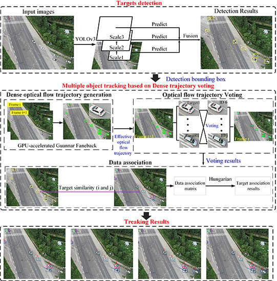
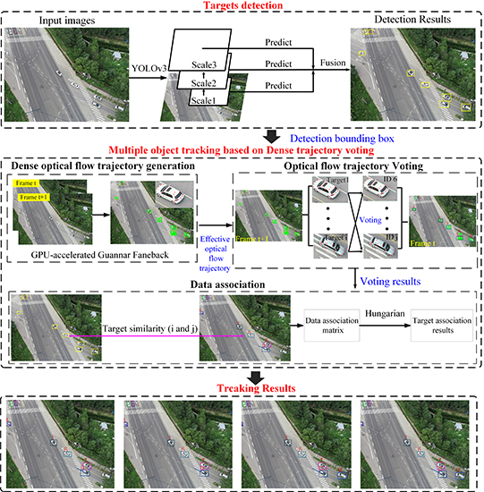
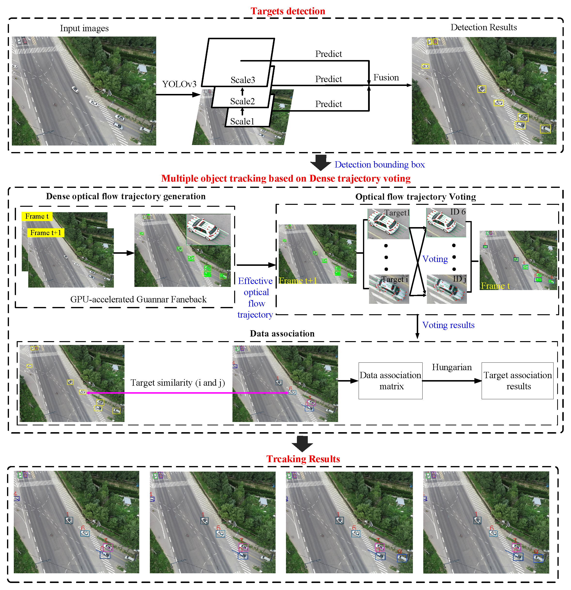
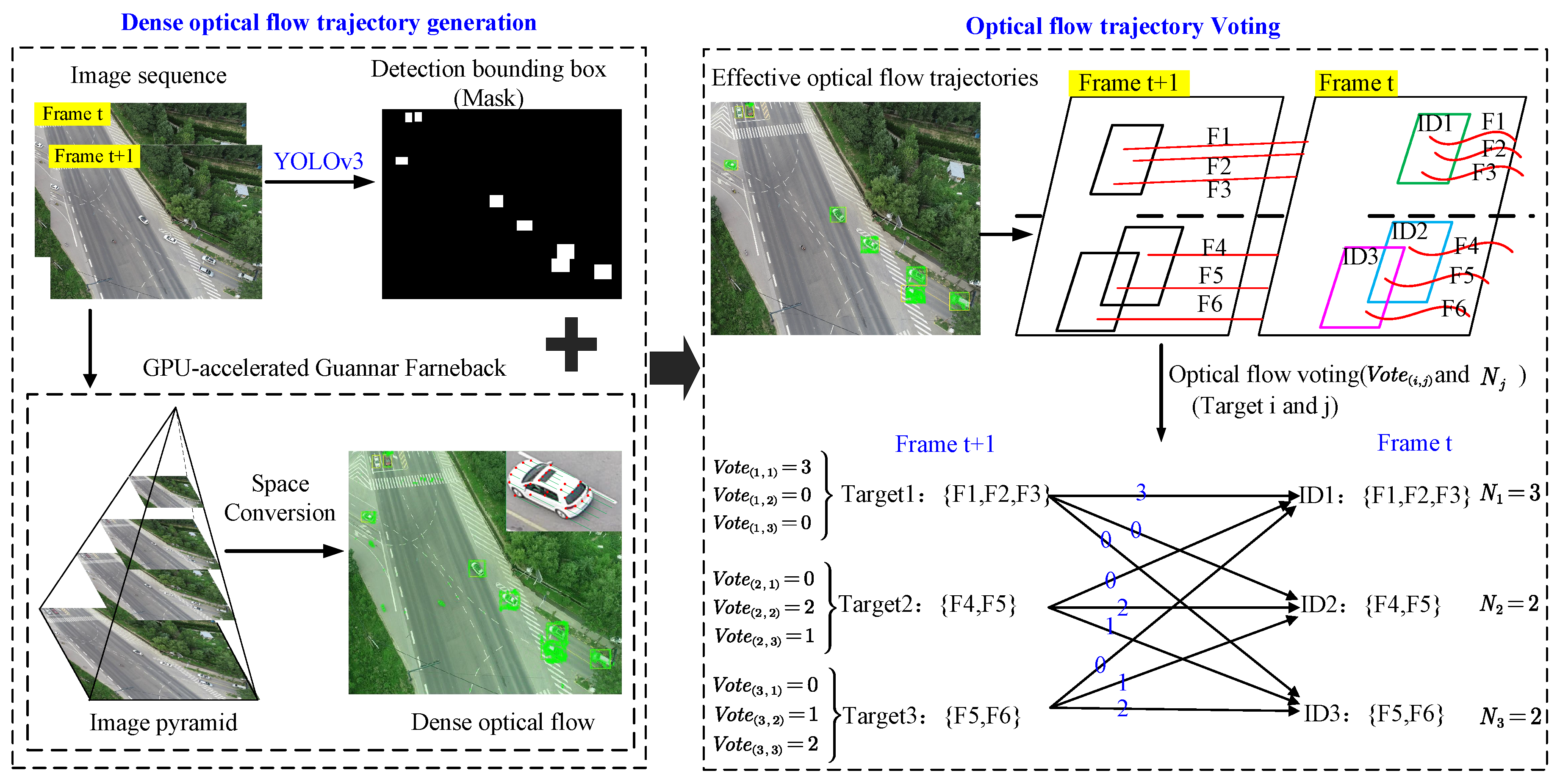
• First of all, we proposed a novel multiple-target-tracking algorithm which is based on dense-optical-flow-trajectory voting. The algorithm models the multiple-target-tracking problem as a voting problem of the dense-optical-flow trajectory to the target ID. In the method, we first generated the optical-flow trajectories of the target and performed ID voting on the optical-flow trajectories of each target. Then, voting results were used to measure the similarity of objects in adjacent frames, and tracking results were obtained by data association. Since the optical-flow trajectory of the target could accurately reflect the position change of the target with time, regardless of the appearance, shape, and size of the target, the algorithm could enhance tracking performance in the aerial video, even at a low frame rate.
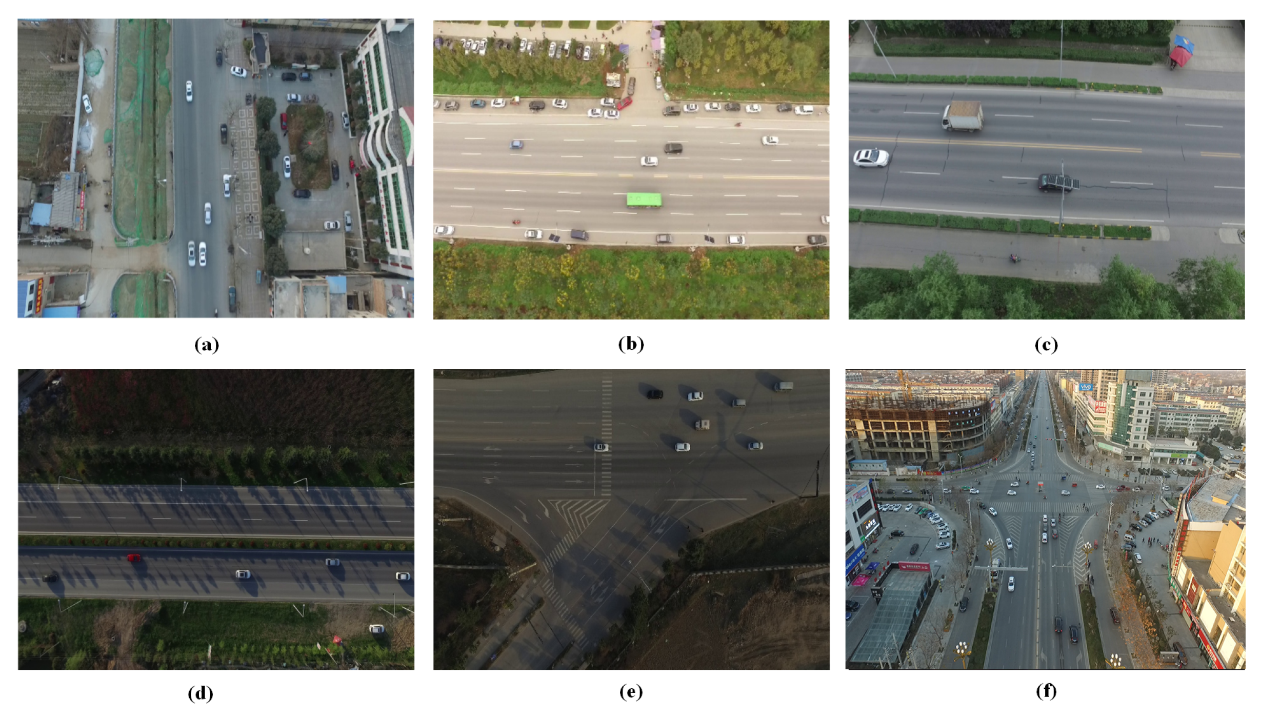
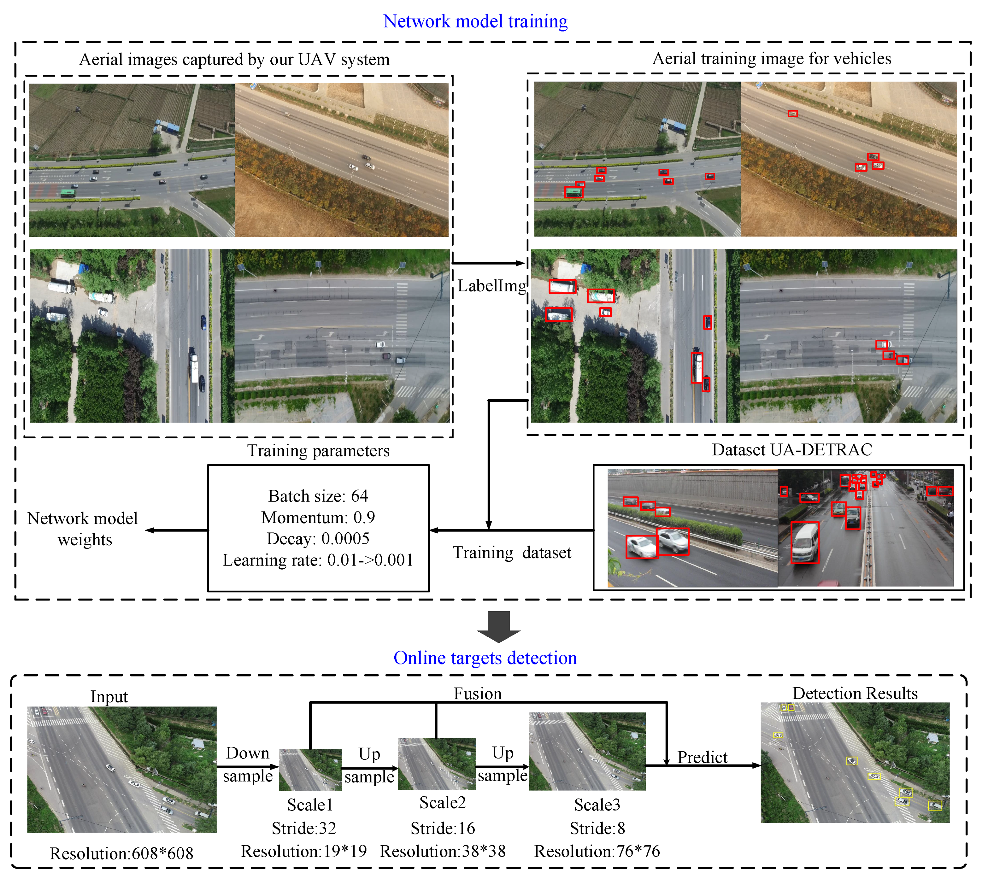
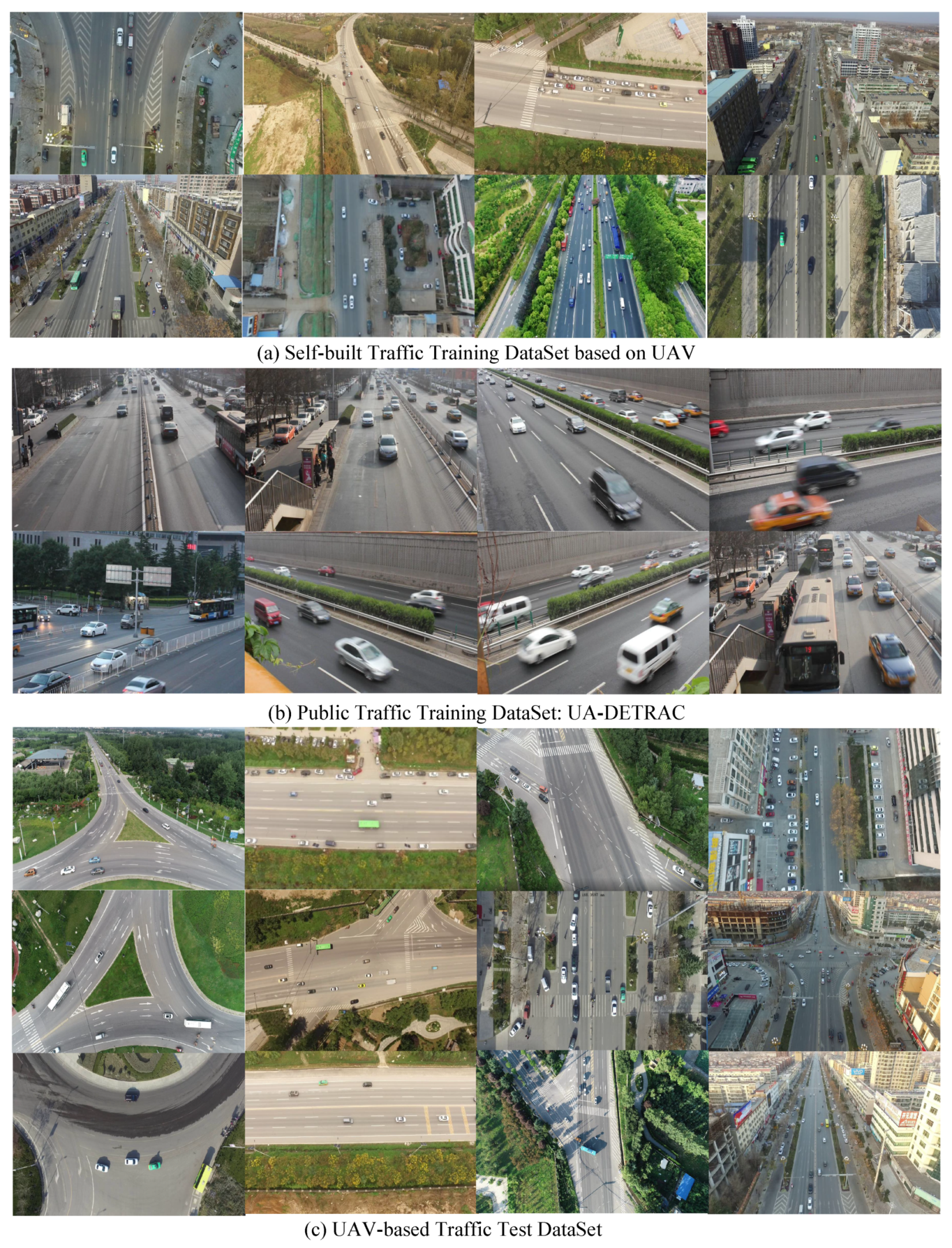
• Second, we built a training dataset and a test dataset for deep-learning vehicle-detection in aerial videos. The training dataset contained many self-captured aerial images, and we used the LabelImg tool to label vehicle targets in these aerial images. The test dataset was collected by our UAV system and included four kinds of surveillance scenarios and multiple video frame rates. The UAV system was composed of DJI-MATRICE 100 and a monocular point-gray camera. Due to the different UAV shooting angles and heights, vehicle sizes in the images are various, and the background is complex. Based on this, we could generate the network model of the deep-learning algorithm and obtain good vehicle-detection results, which is the basis of multiple-target tracking.
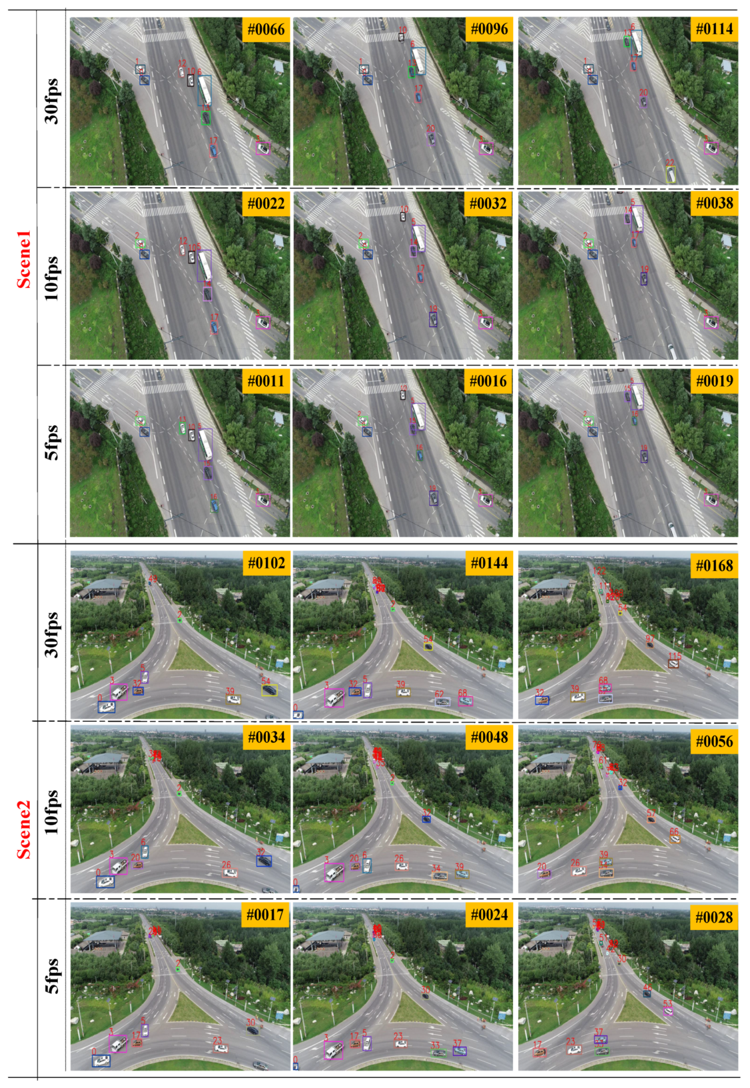
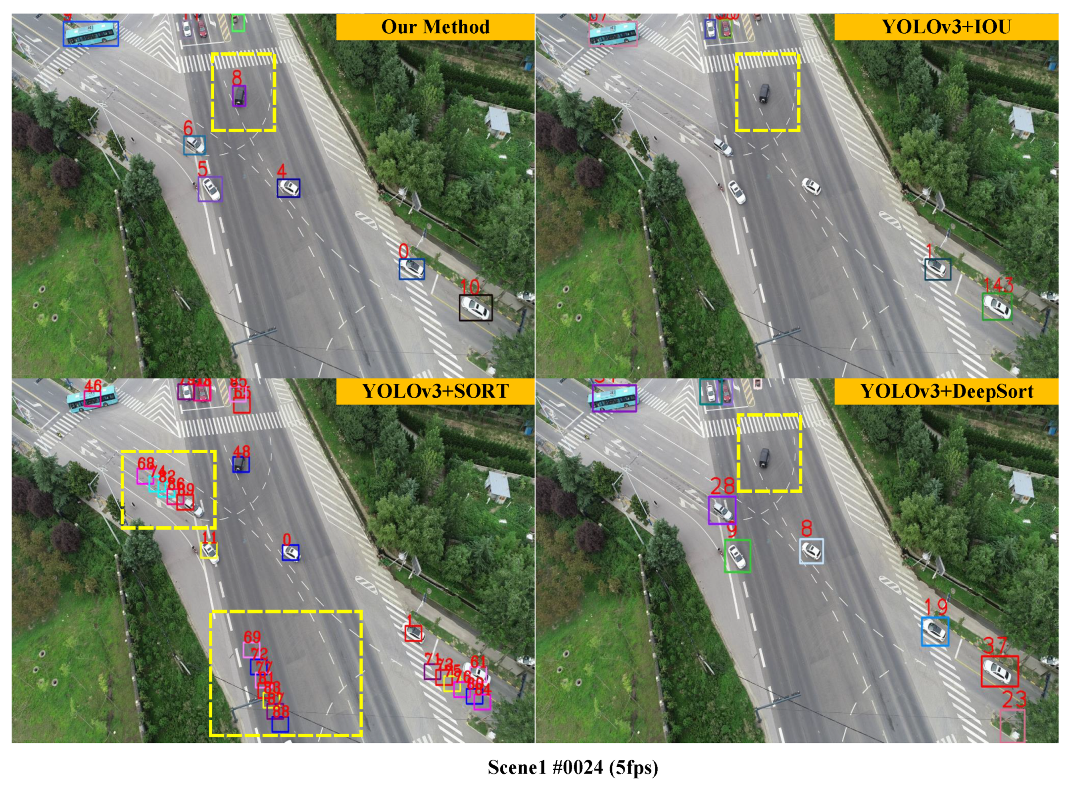
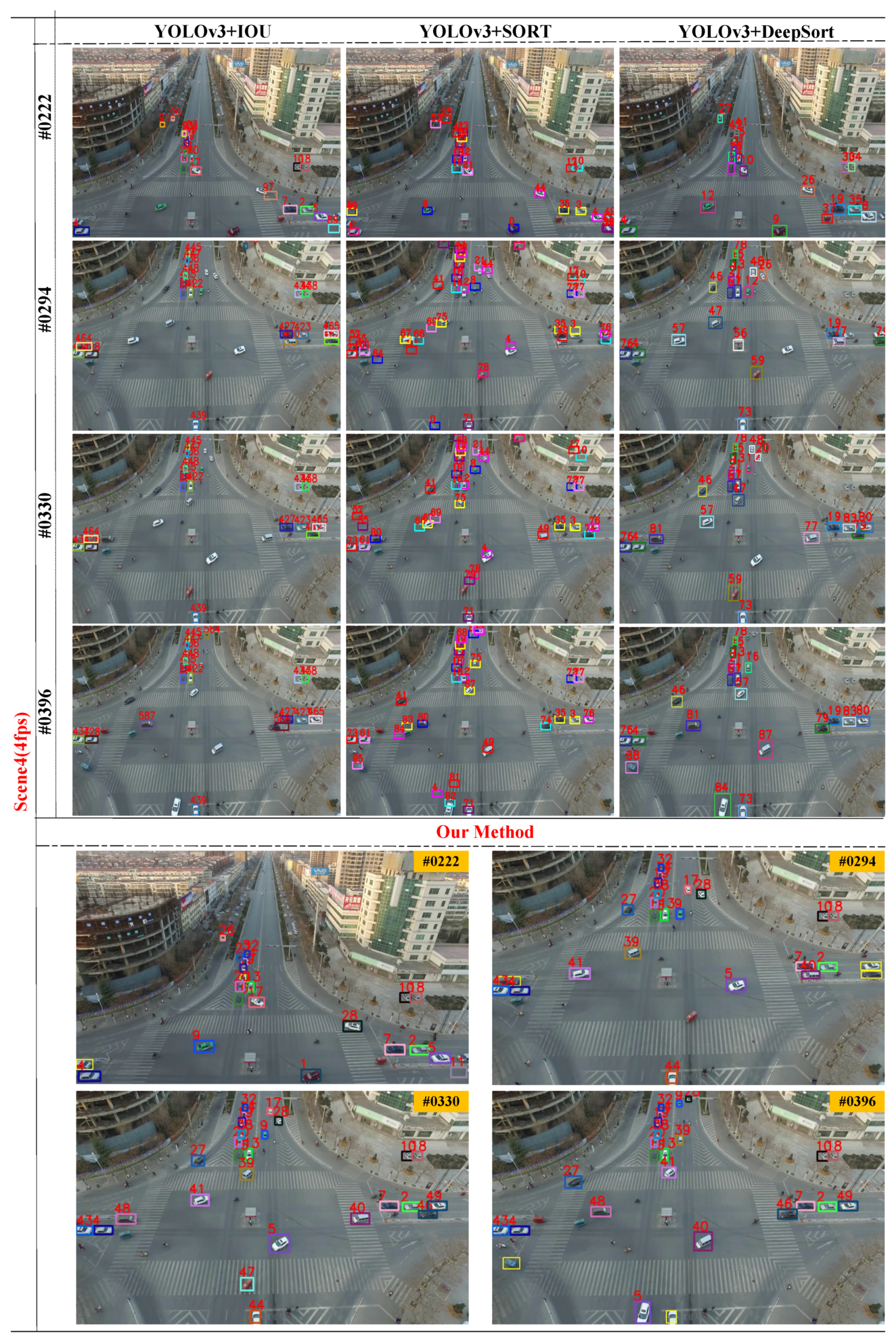
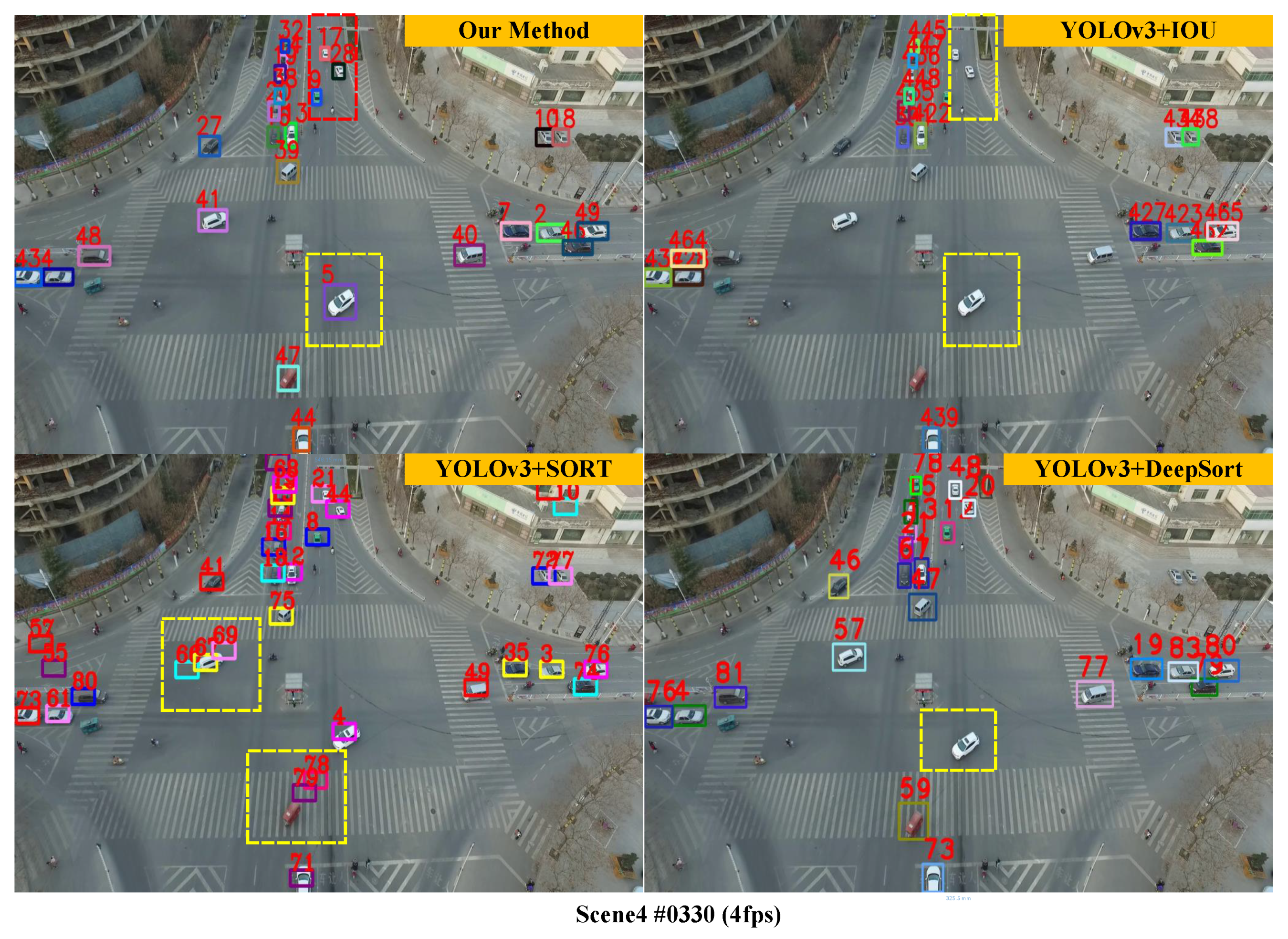
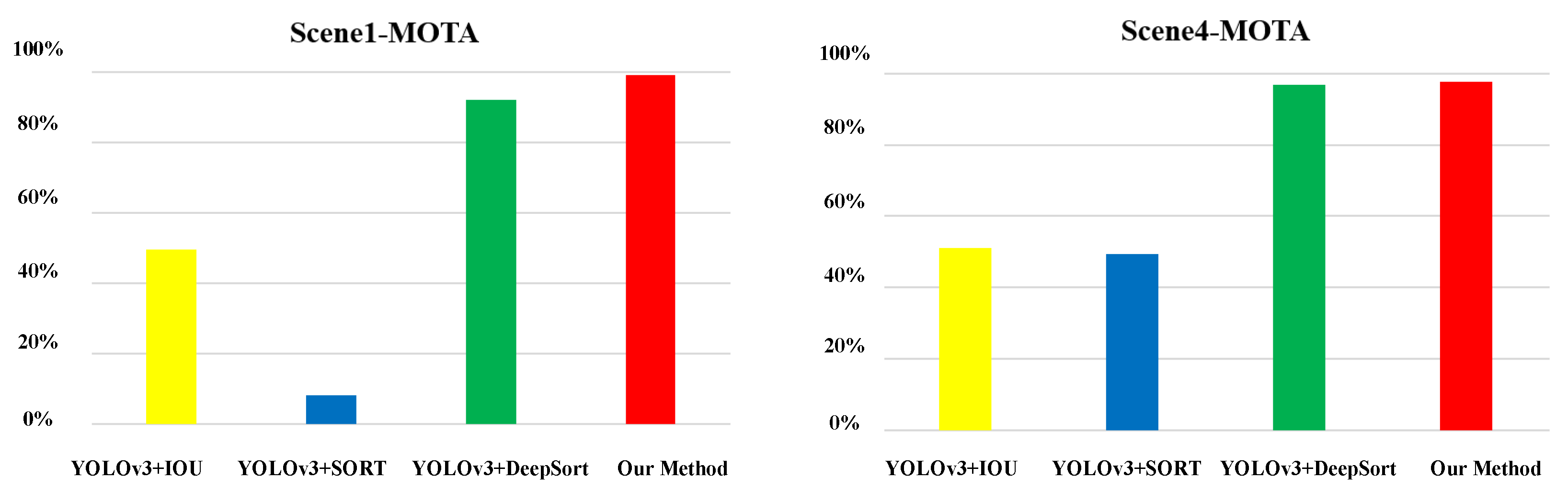
• Finally, we conducted a large number of experiments on the test dataset to prove the effectiveness and robustness of the algorithm. The experiment results on aerial video with various environments and different frame rates show that our algorithm could obtain effective and robust tracking results in various complex environments, and the tracking effect was still robust when there were problems such as target adhesion, low frame rate, and small target size. In addition, we carried out qualitative and quantitative comparison experiments with three state-of-art tracking algorithms, which further proved that this algorithm could not only obtain good tracking results in aerial videos, but also had excellent performance under low frame rate conditions.

2. Proposed Method

A framework of the proposed multiple-target-tracking algorithm based on dense-trajectory voting is shown in Figure 2. The framework can be divided into three parts, target detection, dense-optical-flow-trajectory generation and voting, and data association based on dense-trajectory voting, which are described in the following sections. In the first part, we trained the neural-network model and utilized deep-learning detection algorithm YOLOv3 [26] to obtain the detection bounding box of the vehicle. The method extracted multiple features of images in different scales, then predicted detection bounding boxes and probabilities for each one and fused them to get the final detection result. In the second part, dense-optical-flow-trajectory generation and voting, we first used the GPU-accelerated Gunnar Faneback algorithm to process adjacent frames and obtain the optical flow of each pixel in the current frame. Since we were only interested in the optical-flow trajectories of the targets, effective optical-flow trajectories in the current frame could be generated by combining the detection bounding box. On this basis, according to the target ID of these optical flow trajectories in Frame t, ID voting and statistics are carried out for each target in Frame t + 1 in the process of optical flow trajectory voting. In the third part, we used the voting results to measure the similarity of objects in adjacent frames and generate the data-association matrix. Then, we adopted the Hungarian algorithm [27] to assign the ID of these targets and obtain the tracking results.

2.1. Target Detection

In this part, we outline how we used deep-learning-based detection algorithm YOLOv3 to obtain target position in an aerial image, as shown in the first part of Figure 2. From the input images in Figure 2, we can see that the target scale is small because of the high flying altitude of the drone, and the background is complex. YOLOv2 [28] does not work well for small targets detection, and compared with it, predictions acros scale strategy is added to YOLOv3 algorithm to greatly improve the detection effect of small targets. Compared with FasterRCNN [29] and SSD [30], it not only achieved a good detection effect, but also had the highest speed.

As shown in Figure 3, target detection is divided into the network-model-training and online-target-detection stages. Since the weights provided by the official YOLOv3 website are not good for the detection of small-sized vehicles in airborne videos, we needed to use self-built datasets to train new network-model weights for vehicle detection in aerial images. First, we used our UAV system to collect a large number of aerial images, including a variety of traffic scenes, some of which are shown in Figure 3. The UAV system is composed of a DJI-MATRICE 100 and a monocular point gray camera. Aiming at vehicle targets in aerial images, we utilized LabelImg [31] to generate 5000 annotation files of aerial images; the labeled aerial images are shown in Figure 3. Due to the different UAV shooting angles and heights, vehicle appearance and sizee in these images are various and the background is complex, so that the model they train can have good generalization for new aerial videos. In addition, we supplemented the training dataset with public dataset UA-DETRAC [32]. The dataset had 10,900 images that were captured by a fixed surveillance camera with a high erection height. The vehicle size in these images was medium, similar to aerial images taken by UAVs at low altitude. Based on this training dataset, we chose a YOLOv3 network model for training. The network model included YOLOv3-608, YOLOv3-416, and YOLOv3-302. These models had 106 network layers, but normalized size and speed were different in image processing. Considering the speed and detection effect, we chose to train the YOLOv3-608 network model and obtain the weights. In the process of training, we used a batch size of 64, 0.9 momentum, and 0.0005 decay. The batch size represented the number of sample per batch, which depends on GPU memory. Momentum in the optimization method can affect the speed of gradient descent. Decay is the parameter of weight attenuation that can prevent overfitting. Moreover, we set the initial learning rate, the step of gradient decent, as 0.01, which could rapidly reduce los. Then we changed the learning rate to 0.001 to precisely obtain optimized network-model weights.

After network-model-training, we could perform online vehicle detection in aerial videos. In this process, YOLOv3 regarded the detection problem as a regression problem, and its network architecture adopted hopping connection between non-adjacent layers, and fusion multi-scale features by sampling so that it can get satisfied detection results, including small-sized things. First of all, YOLOv3 normalized resolution of input images to $608\times 608$, since we choose YOLOv3-608 network. Then, YOLOv3 performed down-sampling on the image with a step size of 32, and extracts features to obtain a feature map with $19\times 19$ resolution. Next, two up-samplings are carried out to obtain feature maps of $38\times 38$ and $76\times 76$ respectively, with steps of 16 and 8 relative to the original image. After up-sampling, the receptive field of the convolution layer became smaller and more sensitive to small-sized images. At last, YOLOv3 fused the feature maps of specific scale to get many detection bounding boxes. To filter multiple detection bounding boxes, we used NMS [33] algorithm to leave the most likely one as the final test result.

Briefly, we train the YOLOv3 network model by establishing the training dataset of vehicle targets in aerial images. This model could quickly obtain good target-detection results in aerial videos, which is very important for multiple-object tracking.

2.2. Dense-Optical-Flow-Trajectory Generation and Voting

After target detection, we could obtain detection bounding boxes of the target in the current frame. Then, we needed to determine the ID number of these targets. The optical-flow trajectories of the target could accurately reflect the position change of the target and were still effective when the camera moved. Considering that the optical-flow trajectories of the same target should overlap completely at different times, we used this characteristic of optical-flow trajectories to achieve target tracking in the algorithm.

In this part, we first used the GPU-accelerated Gunnar Farneback algorithm [34] to obtain the optical flow of each pixel in adjacent frames, and combine the detection results to generate effective optical-flow trajectories for each target; dense-optical-flow-trajectory generation is shown in Figure 4. Suppose there are Frames t and t + 1. The Farneback method is a dense-optical-flow algorithm based on gradient. In order to calculate optical flow of all the pixels of Frame t + 1, the algorithm interpolates between easily traceable pixels to generalize to those whose motion is unclear. More precisely, the first step is to calculate the image pyramid. The method observes the image from different scales and calculates the next layer from the information obtained from the previous layer. The advantage is that we could solve the aperture problem, and combine local and overall information. In the second step, each layer of the image pyramid is processed by the algorithm, and the optical-flow field of the image is smoothed by Gaussian blur. Image $I(x,y)$ is modeled by a quadratic polynomial approximately, as follows:

$$I(x,y)\sim {\left[\begin{array}{c}x\\ y\end{array}\right]}^{T}A\left[\begin{array}{c}x\\ y\end{array}\right]+b^T\left[\begin{array}{c}x\\ y\end{array}\right]+c=r1+r_{2}x+r_{3}y+r_4{x}^2+r_5{y}^2+r_{6}xy$$

(1)

where x and y represent abscissa and ordinate in the image-coordinate system, A is a symmetric matrix, b is a vector, and c is a scalar. $r_i$ are coefficients obtained from normalized convolution and Equation (1). The algorithm converts the image to the space where the basis function is $(1,x,y,x^2,y^2,xy)$. We assumed $A_t(x,y),b_t(x,y),c_t(x,y)$ is a polynomial coefficient matrix in frame t. Then,

$$\begin{array}{cc}\hfill (\tilde{x},\tilde{y})& =(x,y)+\tilde{d}(x,y)\hfill \\ \hfill A(x,y)& ={\displaystyle \frac{A_t(x,y)+A_{t+1}(\tilde{x},\tilde{y})}{2}}\hfill \\ \hfill \Delta b(x,y)& =-{\displaystyle \frac{1}{2}}(b_{t+1}(\tilde{x},\tilde{y})-b_t(x,y))+A(x,y)\tilde{d}(x,y)\hfill \end{array}$$

(2)

where $\tilde{d}(x,y)$ is the initial displacement field rounded to integer values, and $(\tilde{x},\tilde{y})$ represents the position predicted in next frame. After that, we set $S(x,y)$ as the scaling matrix, and

$$\begin{array}{cc}\hfill G(x,y)& =S{(x,y)}^{T}A{(x,y)}^{T}A(x,y)S(x,y)\hfill \\ \hfill h(x,y)& =S{(x,y)}^{T}A{(x,y)}^T\Delta b(x,y)\hfill \end{array}$$

(3)

Then, optical-flow field $flow(x,y)$ was calculated as follows:

$$\begin{array}{c}\hfill flow(x,y)=G{(x,y)}^{-1}h(x,y)\end{array}$$

(4)

In this formula, $flow(x,y)$ represents the displacement of pixel $(x,y)$ of Frame t + 1 in the X and Y directions relative to Frame t, and motion relations can be expressed as follows:

$$\begin{array}{c}\hfill Fram{e}^{t+1}(x,y)=Fram{e}^t(x+flow(x,y)\left[0\right],y+flow(x,y)\left[1\right])\\ \hfill whenx+flow(x,y)\left[0\right]<=P,y+flow(x,y)\left[1\right]<=Q,\end{array}$$

(5)

where P and Q represent the length and width of the image, $Fram{e}^{t+1}(x,y)$ represents pixel (x,y) of Frame t + 1, and $Fram{e}^t(x+flow(x,y)\left[0\right],y+flow(x,y)\left[1\right])$ represents pixel $(x+flow(x,y\left)\right[0],y+flow(x,y\left)\right[1\left]\right)$ of Frame t + 1. These two pixels were actually the same pixel at different times. The Farneback method is accurate and robust for calculating optical flow between adjacent frames in aerial videos, and is not restricted by camera motion. It is also applicable when the video frame rate is low. The algorithm is also accelerated by GPU, which improves calculation speed and makes it suitable for practical applications. After obtaining dense-optical-flow information, we used the YOLOv3 detection results as a mask to obtain effective optical flow for the target, as shown in Figure 4.

Thereafter, we voted on the optical-flow trajectories of each target by counting the target ID of these optical-flow trajectories, as shown in Figure 4. Suppose there are three targets in Frame t + 1, Targets 1, 2, and 3. According to the effective optical-flow trajectories of Frame t + 1, we only know which optical-flow trajectories are in each target, but we do not know these targets’ ID. For example, the optical-flow trajectories in Target 1 included F1, F2, and F3. In fact, there are many optical trajectories for a target, at least several hundreds. Because the optical-flow trajectory can be extended in time, we can see that these optical-flow trajectories also existed in Frame t; the target ID of each optical-flow trajectory is known. For instance, optical-flow trajectory F2 belonged to the target of ID 2, and optical-flow trajectory F5 belonged to target of IDs 2 and 3. Based on this information, we voted on the optical-flow trajectories of each target in Frame t + 1, and counted their ID distribution. For example, Target 1 in Frame t + 1 contains optical flows F1, F2, and F3. Because F1 belonged to the target of ID 1, the optical flow voted for the target of ID 1. F2 and F3 also belonged to the target of ID1, and two votes were cast for the target of ID 1. Target 2 in Frame t + 1 contained optical flows F4 and F5. F4 belonged to the target of ID 2, so the optical flow voted for the target of ID 2. F5 belonged to the target of IDs 2 and 3, and voted for the target of IDs 2 and 3. In this paper, we used $Vot{e}_{(i,j)}$ to indicate the vote result, and the value of $Vot{e}_{(i,j)}$ was the number of optical-flow trajectories in target i of Frame t + 1 that belonged to the ID j of Frame t. Therefore, the voting result of Target 1 in Figure 4 is $Vot{e}_{(1,1)}=3,Vot{e}_{(1,2)}=0,Vot{e}_{(1,3)}=0$; the voting result of Target 2 is $Vot{e}_{(2,1)}=0,Vot{e}_{(2,2)}=2,Vot{e}_{(2,3)}=1$. In addition, we needed to count the number of optical flows in each target in Frame t. $N_j$ represents the number of optical flows in the target of ID j in Frame t, such as $N_1=3,N_2=2$.

2.3. Data-Association Based on Dense-Trajectory Voting

When we get the voting results of the optical-flow trajectories of the targets in Frame t + 1, we need to confirm the ID of these targets. The process is shown in Figure 2. In this part, we show data association based on dense-trajectory-voting results. In theory, the optical-flow trajectories of the same target should completely overlap at different times. For example, Target 1 in Frame t + 1 and the target of ID 1 in Frame t contain the optical trajectories of F1, F2 and F3. However, due to some errors in actual optical-flow calculation, the optical-flow trajectories of the same target at different times generally do not completely overlap, but in adjacent frames, the optical-flow overlap ratio between the same targets should be much higher than that of different targets. Based on this, we could use the voting results to measure the similarity of targets between adjacent frames. We assumed that $T_i^{t+1}$ represented target i in Frame t + 1, and $T_j^t$ represented the target of ID j in Frame t. The number of optical-flow trajectories of $T_j^t$ is $N_j$, and the similarity between $T_j^t$ and $T_i^{t+1}$, are calculated as follows:

$$Similarit{y}_{(i,j)}^{(t+1,t)}={\displaystyle \frac{Vot{e}_{(i,j)}}{N_j}}$$

(6)

In this way, we can get the similarity between every two targets in adjacent frames. In order to confirm the matching relationship between the target in Frame t + 1 and the target of the known ID in Frame t, we first used the calculated similarity to generate the data-association matrix of adjacent frames. It was assumed that Frames t+1 and t had M and N detection targets, respectively, and the similarity between $T_i^{t+1}$ and $T_j^t$ was $Similarit{y}_{(i,j)}^{(t+1,t)},i=1,2,3...,M.j=1,2,3,...,N$. Then, we used $NS(i,j)=1-Similarit{y}_{(i,j)}^{(t+1,t)}$ to generate the data-association matrix, as follows:

$$D^{(t+1,t)}=\left[\begin{array}{cccc}NS(1,1)& NS(1,2)& \cdots & NS(1,N)\\ NS(2,1)& NS(2,2)& \cdots & NS(2,N)\\ ⋮& ⋮& \ddots & ⋮\\ NS(M,1)& NS(M,2)& \cdots & NS(M,N)\end{array}\right],$$

(7)

Thereafter, we adopted the Hungarian algorithm to solve the data-association matrix and obtain the optimal target-matching results between Frames t + 1 and t. Then, we needed to further judge whether the two targets were really the same target according to whether the similarity between the matched targets was greater than threshold $TH$. For example, if targets $T_i^{t+1}$ and $T_j^t$ were assigned together by the Hungarian algorithm and their similarity satisfied $Similarit{y}_{(i,j)}^{(t+1,t)}>TH$, targets i and j matched each other and belonged to the same target. This means $I{D}_i^{t+1}=I{D}_j^t$, and $I{D}_i^{t+1}$ represents the ID number of the target $T_i^{t+1}$ in Frame t + 1. Otherwise, it was considered that a new target could emerge, and a new ID was assigned to detection target $T_i^{t+1}$. In the proposed algorithm, we set $TH=0.6$.

In addition, because the YOLOv3 algorithm may have missed targets and false targets, our tracking algorithm adopted a prudent judgment strategy when creating a new target ID and deleting an ID number. For unmatched targets or targets that failed to match in current frame t, we set an observation period for them. When the number of consecutive occurrences of a target in a subsequent frame exceeded the $AN$ frame (observation period), we set it as a new target and assigned a new ID that could reduce false targets generated by the detector. We set $AN$ as 3 in this method. For the unmatched target in previous frame t − 1, we temporarily retained the target in the tracking result of the subsequent $DN$ frames (reservation time), and used optical-flow calculation to update the target position in the current frame. In this paper, $DN=10$. If the target is rematched in the current frame within the reservation time, the target is reidentified as being in the image. Otherwise, the target left the image and destroyed the target ID. This can avoid a detector’s missed detection to a certain extent. The proposed multiple-target algorithm flow is shown in Algorithm 1.

Algorithm 1: Proposed multiple-target-tracking method.

3. Experiment Results

In this section, in order to evaluate the performance of the multiple-object-tracking algorithm presented in this paper, we built an aerial-image dataset for vehicle targets, including a training dataset and a test dataset. Based on the test dataset, we conducted many real experiments to test algorithm performance, including qualitative experiments at different frame rates, and qualitative and quantitative comparison experiments with other state-of-art algorithms.

3.1. Self-Built Dataset of Aerial Images

In this part, we introduce the self-built dataset of the aerial images, including training dataset $Train\_UAVData$, used to train the YOLOv3 network model, and test dataset $Test\_UAVData$ for the performance evaluation of the proposed tracking algorithm.

Self-built training dataset $Train\_UAVData$ for training the YOLOv3 network model had 15,900 images—5000 aerial images and 10,900 pictures of the public traffic dataset UA-DETRAC [32]. Some images are shown in Figure 5a. The aerial images in this dataset were taken by a UAV system in a variety of scenes. The UAV system was composed of DJI-MATRICE 100 and a monocular point gray camera. Due to the different shooting angles and heights of the UAV, vehicle sizes in the images are various and the background was complex. We used the LabelImg [31] tool to label vehicle targets in these aerial images and generate label files for these images. The images of the public traffic dataset UA-DETRAC [32] were captured by a fixed surveillance camera with a high erection height; vehicle size was medium, which was similar to aerial images taken by UAVs at low altitude, as shown in Figure 5b. This public dataset was labeled for vehicle targets and contains label files. In this paper, we used this training dataset to offline-train the YOLOv3 network model to get new weights and improve the vehicle-detection effect in aerial images.

The aerial images in test dataset $Test\_UAVData$ were collected by our UAV system at altitudes of 50 to 60 m, which included four kinds of surveillance scenarios and multiple video frame rates. Specifically, the test images were divided into four groups according to the scenarios, intersection, highway triangular turntable, busy road, and crosroad, as shown in Figure 5c. In these scenarios, the number of vehicles was large, the motion of vehicles was complex, such as straight running and turning, and the size of vehicles varied greatly, which greatly challenged the object-tracking algorithm. Each group of images contained more than 8000 images with a resolution of $1280\times 960$, including three different frame rates. The video frame rates of Scenes 1 and 2 were 30, 10, and 5 fps, respectively, and the video frame rates of Scenes 3 and 4 were 25, 8, and 4 fps, respectively. Each group of images can be used to test the tracking performance and robustness of the algorithm at different frame rates. At present, we posted this dataset on a website: https://frank804.github.io/.

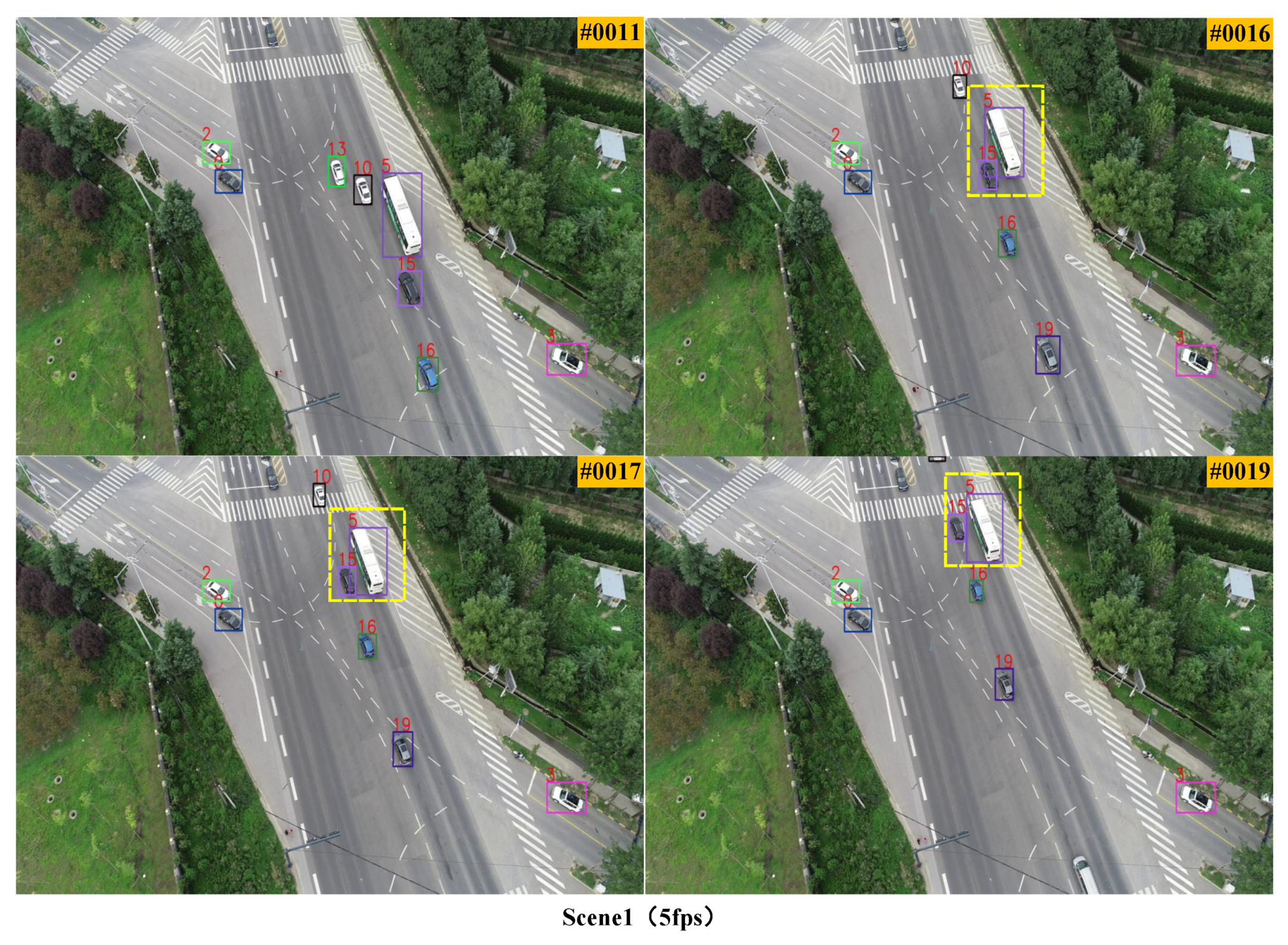
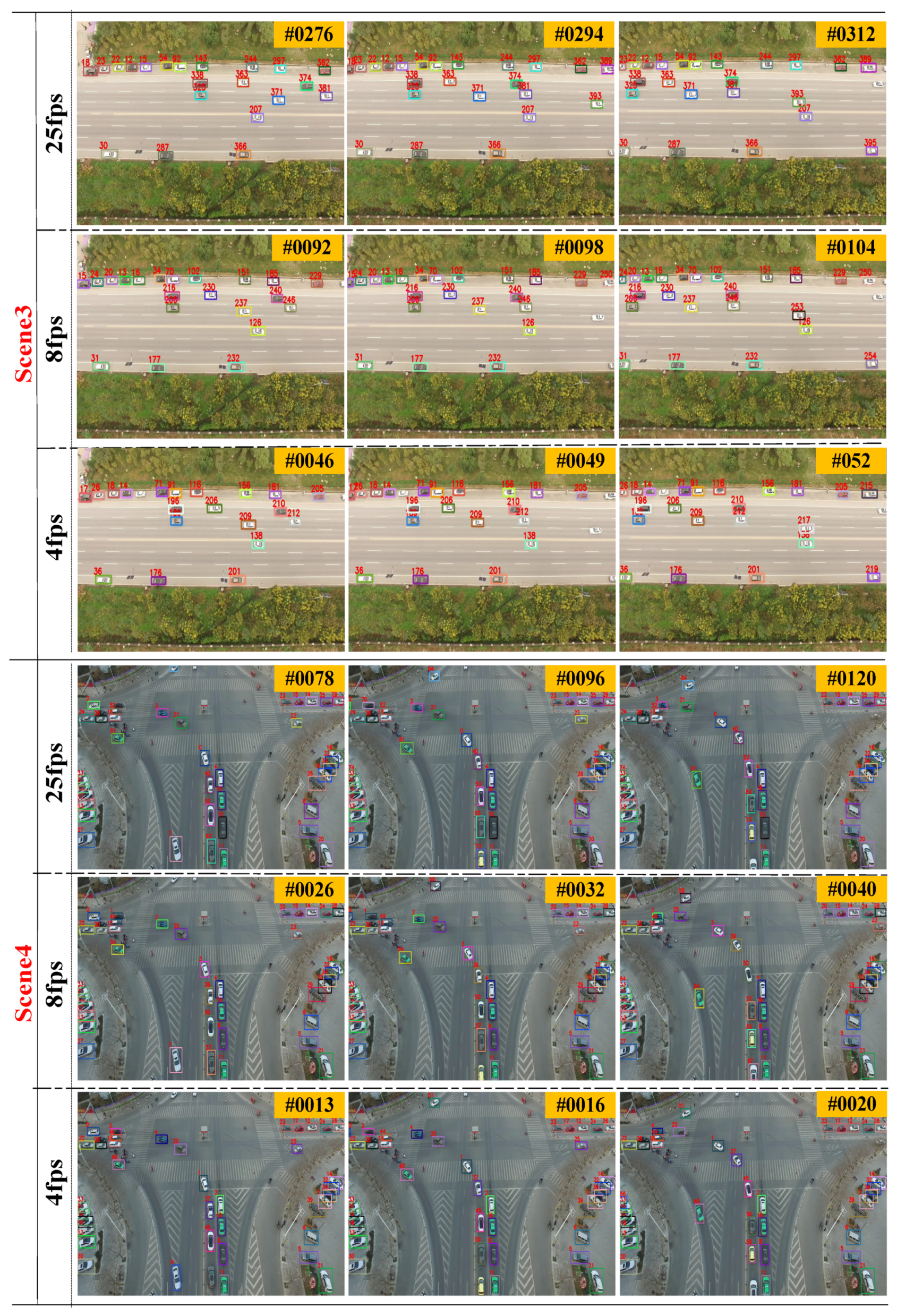
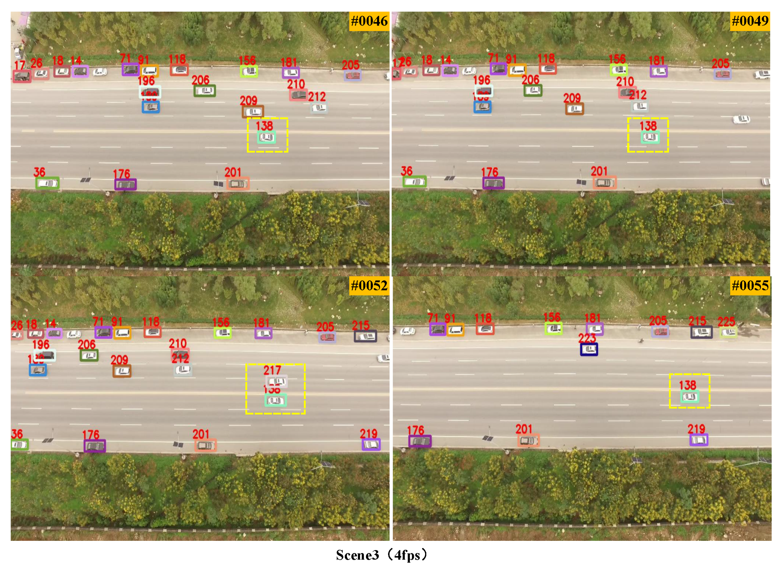
3.2. Qualitative Experiments at Different Frame Rates

In our algorithm, we first used dataset $Train\_UAVData$ to train the YOLOv3 network model, which is used to realize target detection in aerial videos. Based on this, we used the proposed tracking algorithm based on dense-optical-flow-trajectory voting to get multiple-target-tracking results. In this section, we conducted a number of experiments on the test dataset to prove that the proposed multiple-object-tracking algorithm can obtain good tracking results in various complex environments and at different frame rates. From the introduction of the self-built aerial-image dataset above, we can see that the test dataset included four scenes, and each scenario included three different frame rates. The experiment results on this dataset are shown in Figure 6 and Figure 8.

Figure 6 and Figure 7 shows the tracking results at three different frame rates in Scenes 1 and 2. Scene 1 was an intersection and Scene 2 was a highway triangular turntable, and the three frame rates were 30, 10, and 5 fps, respectively. Figure 8 displays the tracking results at three different frame rates in Scenes 3 and 4. Scene 3 was a busy road and Scene 4 was a crosroad, and the three frame rates were 25, 8, and 4 fps. In these scenarios, there were many targets, such as in Scene 1, and the background was complex. There were many trees, solar street lights, and some buildings, such as in Scenes 1 and 2. Target movement was also complicated, for example, stationary, straight driving, turning a corner, turning back, and target size varied greatly.

Despite many difficulties, the proposed tracking method still yielded good results. The results are shown in Figure 6 and Figure 8. For example, (1) the proposed algorithm was able to track targets well in both straight and curved roads at an arbitrary frame rate. Such as Target 13 in Scene 1 of Figure 6, the black vehicle moving in a straight line at 30 fps, Target 14 at 10 fps, Target 15 at 5 fps; Target 39 in Scene 2 of Figure 6, the white vehicle moving along the curve at 30 fps, Target 26 at 10 fps, and Target 23 at 5 fps. (2) Small targets could be tracked correctly, such as Target 2, Target 54 in 30 fps, Target 2, Target 32 in 10 fps, and Target 2, and Target 30 in 5 fps in Scene 2 of Figure 6. (3) The detection and tracking of stationary targets was effective, such as Targets 92, 102, 141 at 25, 8, and 4 fps, respectively, in Scene 3 of Figure 8. (4) At a vehicle-intensive city intersection, the vehicle’s turning and U-turn movements were also likely to cause target tracking to be lost from the curve. Our algorithm can also achieve good tracking results. Such as Target 61 at 4 fps in Scene 4 of Figure 8. (5) The proposed tracking algorithm also worked well for predictive tracking by optical-flow-trajectory voting, such as Target 0 at 25 fps, Target 3 at 8 fps, and Target 1 at 4 fps in Scene 4 of Figure 8. (6) Object adhesion caused by moving vehicles with closer movement, which is very easy to misjudge two targets as one. Such as Target 217 in Scene 3 of Figure 9. However, our tracking algorithm could track them very well by using the optical-flow voting method.

In general, it can be seen that we obtain great tracking performance in a certain number of moving vehicles, which included few error detections and missed detections, and solved the adhesion problem well.

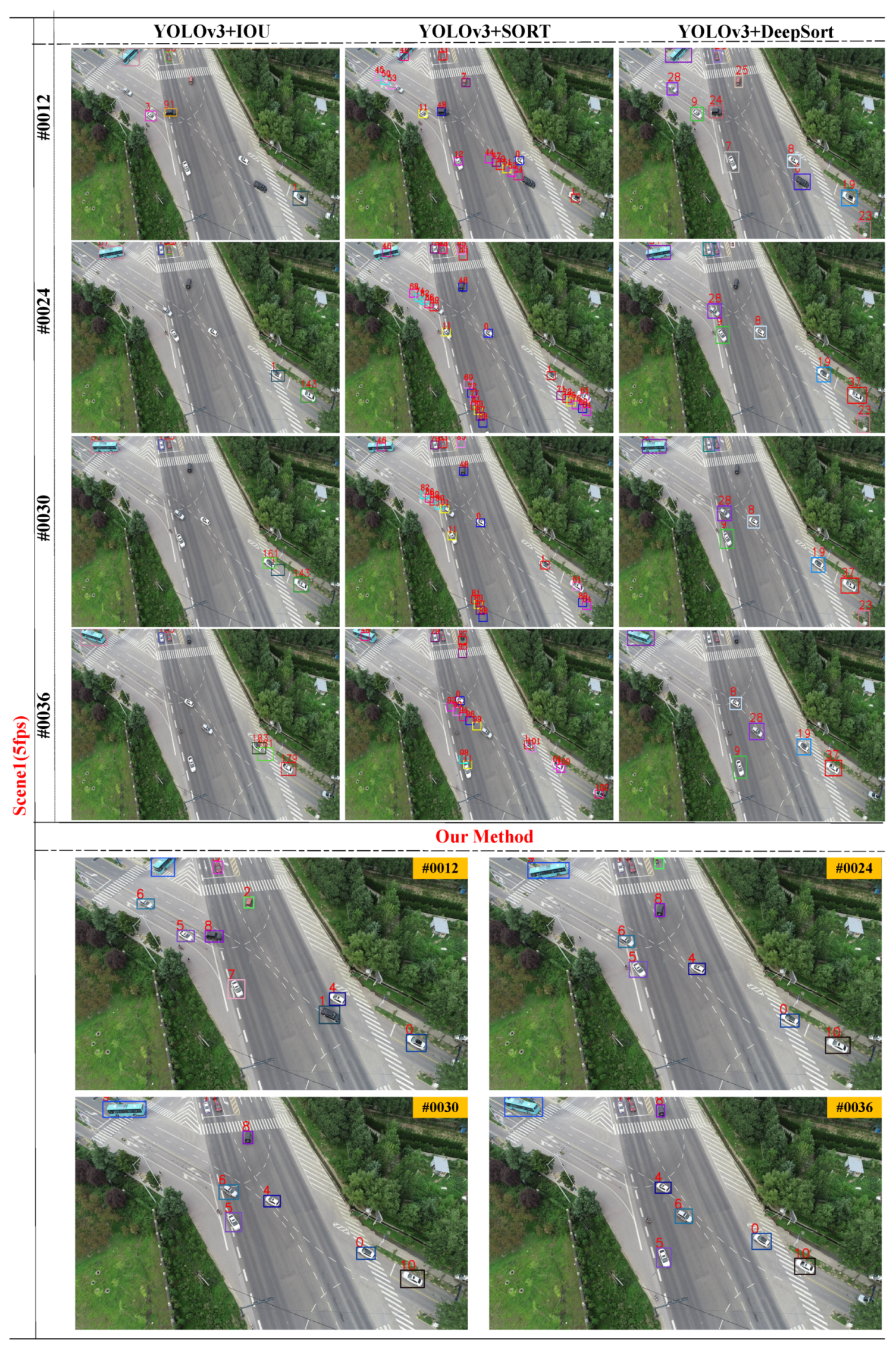
3.3. Qualitative and Quantitative Comparison Experiments

In this section, we outline qualitative and quantitative comparison experiments with three state-of-art tracking algorithms to further evaluate the performance of the proposed multiple-tracking algorithm. These three tracking method were YOLOv3 + IOU [24], YOLOv3 + SORT [21], and YOLOv3 + DeepSort [22], respectively. We selected two scenarios from test dataset $Test\_UAVData$ for the experiment, Scenes 1 and 4, respectively. Scene 1 was an intersection with complex background and vehicle movement. Scene 4 was a crosroad, there were many vehicles in the scene, and the motion of the target was complicated.

After the self-built training dataset was trained for the YOLOv3 network model, deep-learning algorithm YOLOv3 could generally obtain good detection results in various environments. On this basis, YOLOv3 + IOU, YOLOv3 + SORT, and YOLOv3 + DeepSort could generally get good tracking results at a normal frame rate. According to qualitative-experiment analysis above, we can see that the tracking performance of the proposed algorithm was also excellent at normal frame rates. Considering that, in practical applications, due to the limitation of data-transmission bandwidth or the requirement of simultaneous transmission of multichannel videos, it is often necessary to process low-frame-rate videos. Therefore, the tracking performance of a multiple-target-tracking algorithm at low frame rate is also very important. In the comparative experiment, we tested these four algorithms for low-frame-rate videos, and the frame rate was 5 fps. The experiment results in Scenes 1 and 4 are shown in Figure 10, Figure 11, Figure 12 and Figure 13. In addition, we quantitatively analyzed the tracking performance of the four algorithms. Commonly used performance-evaluation parameters for multiple-target tracking include FP, the number of false positives; FN, the number of missed targets; IDs, the number of target ID changes; and MOTA [35], that intuitively express a tracker’s overall strengths and the calculation formula is given by:

$$MOTA=1-\frac{\sum FN+FP+IDs}{Total}$$

(8)

where Total indicates the number of objects present in the image.

In the video with 5 fps frame rate in Scenes 1 and 4, we selected 200 consecutive images in each scene for parameter statistics. The tracking-performance parameters of the four tracking methods are shown in

Table 1. Tracking performance parameters of four tracking methods.

Methods	Scene1					Scene4
	Total	FP	FN	IDs	MOTA(%)	Total	FP	FN	IDs	MOTA(%)
YOLOv3+IOU [24]	1888	72	824	56	49.57	2956	120	1010	314	51.15
YOLOv3+SORT [21]	1888	1448	74	214	8.05	2956	1302	84	106	49.52
YOLOv3+DeepSort [22]	1888	80	362	10	91.94	2956	10	60	20	96.95
Our Method	1888	2	14	4	98.94	2956	4	62	6	97.56

.

The YOLOv3 + IOU method relies on the coincidence area of adjacent frame targets. Since low-frame-rate detection caused the target to have a large interval in adjacent frames and a small overlap area, especially in Scene 4 of Figure 12, the camera lens performed a vertical rotation motion, so the tracking effect was poor and the FN was large. In order to solve the problem of high-speed moving-target tracking, we constructed an image multiresolution wavelet pyramid in our optical flow system and obtained displacement at different scales. The displacement of the gold-tower layer and interlayer-displacement calculation were used to Reduce the displacement on different scales compared to the original displacement. Therefore, it could still track well at low frame rates or high-speed motion.

The YOLOv3 + SORT method relies on Kalman prediction and target area coincidence degree judgment, so vehicle targets were easy to deviate from the curve trajectory tracking in the fast-turning situation. For example, the tracking frame of white vehicle Target 4 in Scene 4 of Figure 12 seriously deviated from the normal trajectory when cornering. Since low frame rate causes the adjacent frame target spacing to be too large, YOLOv3 + SORT could easily lose the target and retrack it as a new target.

On the other hand, tracking lost targets is reserved for multiple frames for prediction. As a result, rapidly moving vehicle targets are mistaken for a plurality of new targets, resulting in an increase in FP value. For example, (1) black-vehicle Targets 44–54 in Scene 1 of Figure 10. (2) silver-car Targets 65–75 in Scene 4 of Figure 12. In view of the fact that a target is easy to lose when turning, our optical-flow-tracking system directly obtained the motion information of the target in the historical frame, so the target could accurately track the curve motion.

The YOLOv3 + DeepSort method relies on previously identified target features for re-recognition, so it is easy to lose targets when target detection is poor and appearance changes rapidly at low frame rates. For example, (1) in Scene 1 of Figure 10, black-vehicle Target 24 made a wide 90 degree turn, and white-vehicle Target 10 in Scene 4 of Figure 12 made a 180 degree sharp turn. The appearance of the vehicle changed quickly from the side view to the rear view. (2) In Scene 4 of Figure 12, vehicles 8 and 77 passed through the intersection center because they had multiple frames to detect lost targets and vehicle-angle changes, and were reidentified as Targets 84 and 87.

Compared with the three other algorithms in Table 1, the FP and FN values of our method were relatively small. Performance parameter MOTA was 98.94% and 97.56% in Scenes 1 and 4, which were better than the other three algorithms, as shown in Figure 14. Although our system has many processing mechanisms, there were some targets which could not be tracked well. This was mainly because some targets had not been detected for a long time and could not produce target-tracking results.

Additionally, we tested the time performance of the proposed tracking algorithm. The used computer had an Intel i5-8400 CPU, 8 GB RAM, an Nvidia GeForce GTX1080Ti GPU, and 6 GB video memory. The algorithm was implemented by two processes. One process was the YOLOv3 algorithm, and its average calculation time was 46.0 ms. The other process was target tracking, with an average time of about 93.2 ms, including optical-flow-trajectory generation, voting, and data association. The two processes can run at the same time. With extra time such as coping images, resizing images and so on, the average processing time of the algorithm for image processing at $1920\times 1080$ resolution is 115.4 ms, higher than 93.2 ms slightly. Therefore, the proposed tracking algorithm could be fast, efficient, and robust, and is suitable for practical scenarios.

In addition to the vehicle-tracking results presented in the paper, we also produced a video demo with more experiment results to demonstrate the effectiveness and robustness of our tracking algorithm, which you can review in the Supplementary Material. Moreover, we have posted the code and the demo for multiple objects tracking algorithm based on dense trajectories voting in aerial videos on a website: https://frank804.github.io/.

4. Conclusions

In this paper, we proposed a novel multiple-object-tracking algorithm based on dense-trajectory voting in aerial videos. The core of the algorithm was to obtain target-tracking results by voting the target ID on target-optical-flow trajectories, which is superior to obtain good tracking results in various complex aerial environments and at different frame rates. More specifically, we first built training dataset $Train\_UAVData$ of aerial images and used the YOLOv3 algorithm to obtain vehicle-detection results in aerial videos. Then, combined with the detection results, we utilized a GPU-accelerated Gunnar Farneback algorithm to process the adjacent frames and generate effective target-optical-flow trajectories. On this basis, according to the target ID of these optical-flow trajectories, ID voting and statistics were carried out for each target. After that, we used the voting results to measure the similarity between detection objects in adjacent frames and obtain the tracking results through data association.

Finally, in order to evaluated the tracking performance of this method, we conducted a number of experiments on the self-built test dataset $Test\_UAVData$, including qualitative experiments at different frame rates, and qualitative and quantitative comparison experiments with other state-of-art algorithms. A large number of experiment results verified that the proposed tracking algorithm could work in various complex environments at different frame rates, and obtain effective and robust tracking results when there are some situations such as target adhesion, large changes of target size, complex backgrounds, similar target appearance, and complicated motion of targets. In addition, compared with the three other advanced tracking algorithms, the tracking effect of YOLOv3 + IOU and YOLOv3 + SORT is greatly reduced by low video frame rates, and their MOTA was less than 50%, while our tracking algorithm was robust in low-frame-rate aerial videos, the MOTA was about 98%, and performance was much better than the other algorithms.

References

1. Kumar, R.; Sawhney, H.; Samarasekera, S.; Hsu, S.; Tao, H.; Guo, Y.; Hanna, K.; Pope, A.; Wildes, R.; Hirvonen, D. Aerial video surveillance and exploitation. Proc. IEEE 2001, 89, 1518–1539. [Google Scholar] [CrossRef]
2. Yang, T.; Li, Z.; Zhang, F.; Xie, B.; Li, J.; Liu, L. Panoramic uav surveillance and recycling system based on structure-free camera array. IEEE Access 2019, 7, 25763–25778. [Google Scholar] [CrossRef]
3. Ke, R.; Li, Z.; Kim, S.; Ash, J.; Cui, Z.; Wang, Y. Real-Time Bidirectional Traffic Flow Parameter Estimation From Aerial Videos. IEEE Trans. Intell. Transp. Syst. 2017, 18, 890–901. [Google Scholar] [CrossRef]
4. Zhao, X.; Pu, F.; Wang, Z.; Chen, H.; Xu, Z. Detection, Tracking, and Geolocation of Moving Vehicle From UAV Using Monocular Camera. IEEE Access 2019, 7, 101160–101170. [Google Scholar] [CrossRef]
5. Cao, X.; Jiang, X.; Li, X.; Yan, P. Correlation-Based Tracking of Multiple Targets With Hierarchical Layered Structure. IEEE Trans. Cybern. 2018, 48, 90–102. [Google Scholar] [CrossRef] [PubMed]
6. Bi, F.; Lei, M.; Wang, Y.; Huang, D. Remote Sensing Target Tracking in UAV Aerial Video Based on Saliency Enhanced MDnet. IEEE Access 2019, 7, 76731–76740. [Google Scholar] [CrossRef]
7. Farmani, N.; Sun, L.; Pack, D.J. A Scalable Multitarget Tracking System for Cooperative Unmanned Aerial Vehicles. IEEE Trans. Aerosp. Electron. Syst. 2017, 53, 1947–1961. [Google Scholar] [CrossRef]
8. Bhattacharya, S.; Idrees, H.; Saleemi, I.; Ali, S.; Shah, M. Moving object detection and tracking in forward looking infra-red aerial imagery. In Machine Vision Beyond Visible Spectrum; Springer: Berlin/Heidelberg, Germany, 2011; pp. 221–252. [Google Scholar]
9. Andres, B.; Kroeger, T.; Briggman, K.L.; Denk, W.; Korogod, N.; Knott, G.; Koethe, U.; Hamprecht, F.A. Globally Optimal Closed-Surface Segmentation for Connectomics. In Proceedings of the European Conference on Computer Vision, Florence, Italy, 7–13 October 2012; pp. 778–791. [Google Scholar]
10. Uzkent, B.; Hoffman, M.J.; Vodacek, A. Real-Time Vehicle Tracking in Aerial Video Using Hyperspectral Features. In Proceedings of the Computer Vision and Pattern Recognition Workshops, Las Vegas, NV, USA, 26 June–1 July 2016; pp. 1443–1451. [Google Scholar]
11. Liu, X.; Yang, T.; Li, J. Real-Time Ground Vehicle Detection in Aerial Infrared Imagery Based on Convolutional Neural Network. Electronics 2018, 7, 78. [Google Scholar] [CrossRef]
12. Ochs, P.; Malik, J.; Brox, T. Segmentation of Moving Objects by Long Term Video Analysis. IEEE Trans. Pattern Anal. Mach. Intell. 2014, 36, 1187–1200. [Google Scholar] [CrossRef] [PubMed]
13. Keuper, M.; Andres, B.; Brox, T. Motion Trajectory Segmentation via Minimum Cost Multicuts. In Proceedings of the IEEE International Conference on Computer Vision, Santiago, Chile, 7–13 December 2015; pp. 3271–3279. [Google Scholar]
14. Li, J.; Dai, Y.; Li, C.; Shu, J.; Li, D.; Yang, T.; Lu, Z. Visual Detail Augmented Mapping for Small Aerial Target Detection. Remote. Sens. 2019, 11, 14. [Google Scholar] [CrossRef]
15. Xiao, J.; Cheng, H.; Sawhney, H.; Han, F. Vehicle detection and tracking in wide field-of-view aerial video. In Proceedings of the Computer Vision and Pattern Recognition, San Francisco, CA, USA, 13–18 June 2010; pp. 679–684. [Google Scholar]
16. Szottka, I.; Butenuth, M. Tracking multiple vehicles in airborne image sequences of complex urban environments. In Proceedings of the Urban Remote Sensing Event, Munich, Germany, 11–13 April 2011; pp. 13–16. [Google Scholar]
17. Wang, Y.; Zhang, Z.; Wang, Y. Moving Object Detection in Aerial Video. In Proceedings of the International Conference on Machine Learning and Applications, Boca Raton, FL, USA, 12–15 December 2012; pp. 446–450. [Google Scholar]
18. Al-Kaff, A.; Gómez-Silva, M.J.; Moreno, F.M.; de la Escalera, A.; Armingol, J.M. An appearance-based tracking algorithm for aerial search and rescue purposes. Sensors 2019, 19, 652. [Google Scholar] [CrossRef] [PubMed]
19. Chen, T.; Pennisi, A.; Li, Z.; Zhang, Y.; Sahli, H. A Hierarchical Association Framework for Multi-Object Tracking in Airborne Videos. Remote. Sens. 2018, 10, 1347. [Google Scholar] [CrossRef]
20. Yin, Y.; Wang, X.; Xu, D.; Liu, F.; Wang, Y.; Wu, W. Robust visual detection—learning—tracking framework for autonomous aerial refueling of UAVs. IEEE Trans. Instrum. Meas. 2016, 65, 510–521. [Google Scholar] [CrossRef]
21. Bewley, A.; Ge, Z.; Ott, L.; Ramos, F.; Upcroft, B. Simple online and realtime tracking. In Proceedings of the 2016 IEEE International Conference on Image Processing, Phoenix, AZ, USA, 25–28 September 2016; pp. 3464–3468. [Google Scholar]
22. Wojke, N.; Bewley, A.; Paulus, D. Simple Online and Realtime Tracking with a Deep Association Metric. In Proceedings of the 2017 IEEE International Conference on Image Processing, Beijing, China, 17–20 September 2017; pp. 3645–3649. [Google Scholar]
23. Wojke, N.; Bewley, A. Deep Cosine Metric Learning for Person Re-identification. In Proceedings of the 2018 IEEE Winter Conference on Applications of Computer Vision (WACV), Lake Tahoe, NV, USA, 12–15 March 2018; pp. 748–756. [Google Scholar]
24. Bochinski, E.; Eiselein, V.; Sikora, T. High-speed tracking-by-detection without using image information. In Proceedings of the IEEE International Conference on Advanced Video and Signal Based Surveillance, Lecce, Italy, 29 August–1 September 2017; pp. 1–6. [Google Scholar]
25. Zhou, H.; Kong, H.; Wei, L.; Creighton, D.; Nahavandi, S. Efficient Road Detection and Tracking for Unmanned Aerial Vehicle. IEEE Trans. Intell. Transp. Syst. 2015, 16, 297–309. [Google Scholar] [CrossRef]
26. Redmon, J.; Farhadi, A. YOLOv3: An Incremental Improvement. CoRR. 2018. Available online: http://xxx.lanl.gov/abs/1804.02767 (accessed on 1 March 2019).
27. Kuhn, H.W. The Hungarian method for the assignment problem. Nav. Res. Logist. Q. 1955, 2, 83–97. [Google Scholar] [CrossRef] [Green Version]
28. Redmon, J.; Farhadi, A. YOLO9000: Better, faster, stronger. In Proceedings of the IEEE Conference on Computer Vision and Pattern Recognition, Honolulu, HI, USA, 21–26 July 2017; pp. 7263–7271. [Google Scholar]
29. Ren, S.; He, K.; Girshick, R.; Sun, J. Faster r-cnn: Towards real-time object detection with region proposal networks. In Advances in Neural Information Processing Systems; 2015; pp. 91–99. Available online: https://papers.nips.cc/paper/5638-faster-r-cnn-towards-real-time-object-detection-with-region-proposal-networks.pdf (accessed on 1 March 2019).
30. Liu, W.; Anguelov, D.; Erhan, D.; Szegedy, C.; Reed, S.; Fu, C.; Berg, A.C. SSD: Single shot multibox detector. In Proceedings of the European Conference on Computer Vision, Amsterdam, The Netherlands, 8–16 October 2016; Springer: Berlin/Heidelberg, Germany, 2016; pp. 21–37. [Google Scholar]
31. Tzutalin. LabelImg. Available online: https://github.com/tzutalin/labelImg (accessed on 1 March 2019).
32. UA-DETRAC. Available online: http://detrac-db.rit.albany.edu/ (accessed on 1 March 2019).
33. Hosang, J.; Benenson, R.; Schiele, B. Learning Non-maximum Suppression. In Proceedings of the IEEE Conference on Computer Vision and Pattern Recognition (CVPR), Honolulu, HI, USA, 21–26 July 2017; pp. 6469–6477. [Google Scholar]
34. Farneback, G. Two-Frame Motion Estimation Based on Polynomial Expansion. In Proceedings of the Scandinavian Conference on Image Analysis, Halmstad, Sweden, 29 June–2 July 2003; pp. 363–370. [Google Scholar]
35. Bernardin, K.; Stiefelhagen, R. Evaluating Multiple Object Tracking Performance: The CLEAR MOT Metrics. EURASIP J. Image Video Process. 2008, 2008, 246309. [Google Scholar] [CrossRef]
Figure 1. Aerial images captured from our Unmanned Aerial Vehicle (UAV) system, including a variety of complex scenes posing various challenges for target tracking: (a) adhesion occurring between two adjacent cars, (b) massive vehicles on side of the road, (c) complex background, (d) many tree shadows, (e) small target size and similar target appearance, (f) large changes in target size and complicated target movement.
Remotesensing 11 02278 g001
Figure 2. Overview of proposed multiple-object-tracking algorithm based on dense-trajectory voting in aerial videos. The algorithm mainly consists of two sections, target detection and object tracking based on dense-trajectory voting. Object tracking includes dense-optical-flow-trajectory generation and voting, and data association based on dense-trajectory voting.
Remotesensing 11 02278 g002
Figure 3. Target-detection process, including offline network-model training and online target detection. In network-model training, the original aerial image was labeled by labelImage, and a training dataset for vehicle target was established. Based on this dataset, we chose a YOLOv3 network model for training. In online target detection, we can obtain a series of target-detection bounding boxes by using training network-model weights.
Remotesensing 11 02278 g003
Figure 4. Dense-optical-flow-trajectory generation and voting process. In this paper, we combined a GPU-accelerated Gunnar Farneback algorithm with detection results to generate effective optical-flow trajectories. To represent the voting process, we assumed that there were three detection targets in Frame t + 1, and the optical-flow trajectories of these targets were { F 1 , F 2 , F 3 } , { F 4 , F 5 } , { F 5 , F 6 } , respectively.
Remotesensing 11 02278 g004
Figure 5. The training dataset T r a i n _ U A V D a t a included self-built training dataset (a) and public traffic training dataset (b). T e s t _ U A V D a t a (c) has images which were taken by us using a drone equipped with a point gray monocular camera in a variety of scenes.
Remotesensing 11 02278 g005
Figure 6. Tracking results at three different frame rates in Scenes 1 and 2. Scene 1 is an intersection and Scene 2 is a highway triangular turntable. In these two scenarios, the background was complex and there were many trees. Target movement was also complicated, such as straight driving and turning a corner, and target size greatly varied.
Remotesensing 11 02278 g006
Figure 7. Tracking results of four tracking algorithms in Scene 1 with 5 fps frame rate, enlarged to show tracking effect more clearly. This set of results mainly shows that the algorithm could track crowded targets well when the frame rate of the intersection was only 5 frames.
Remotesensing 11 02278 g007
Figure 8. Tracking results at three different frame rates in Scenes 3 and 4. Scene 3 is a busy road and Scene 4 is a crosroad. There were many targets in these two scenarios that were prone to target adhesion. Moving state of the target was also complex, such as stationary, straight driving, turning a corner, and turning back.
Remotesensing 11 02278 g008
Figure 9. Tracking results of four tracking algorithms in Scene 3 with 4 fps frame rate, enlarged to show tracking effect more clearly. This set of results mainly show that the algorithm of this paper could track high-speed moving vehicles well when acquisition frame rate was only 4 frames on the highway.
Remotesensing 11 02278 g009
Figure 10. Tacking results of this algorithm and three other tracking algorithms, YOLOv3 + IOU, YOLOv3 + SORT, and YOLOv3 + DeepSort, in Scene 1. Scene 1 was an intersection with a complex background and vehicle movement, and the video frame rate of the experimental images was 5 fps.
Remotesensing 11 02278 g010
Figure 11. Tracking results of four tracking algorithms in Scene 1 with frame rate of 5 fps, enlarged to show the tracking effect more clearly. Scene 1 was an intersection with a complex background and vehicle movement. This set of results showed that YOLOv3 + SORT easily lost the target and entered the prediction stage, causing target ID to be frequently replaced.
Remotesensing 11 02278 g011
Figure 12. Tracking results of this algorithm and three other tracking algorithms in Scene 4, YOLOv3 + IOU, YOLOv3 + SORT, and YOLOv3 + DeepSort. Scene 4 was a crosroad, there were many vehicles in the scene, and the motion of the target was complicated. The video frame rate of the experimental images was 5 fps.
Remotesensing 11 02278 g012
Figure 13. Tracking results of the four tracking algorithms in Scene 4 with frame rate of 5 fps, which are enlarged to show the tracking effect more clearly. Scene 4 is a crosroad, there are many vehicles in the scene, and the motion of the target is complicated. This set of results show that YOLOv3 + DeepSort easily lost the target when the target turned.
Remotesensing 11 02278 g013
Figure 14. Histogram of tracking-performance parameter MOTA of four tracking methods. The MOTA of: YOLOv3 + IOU in Scenes 1 and 4 was 98.94% and 97.56%, YOLOv3 + SORT in Scenes 1 and 4 was 98.94% and 97.56%, and YOLOv3 + DeepSort in Scenes 1 and 4 was 98.94% and 97.56%. The MOTA of our method was 98.94% and 97.56% in Scenes 1 and 4, which was better than the three other algorithms.
Remotesensing 11 02278 g014