Seasonal Evaluation of SMAP Soil Moisture in the U.S. Corn Belt

Abstract

NASA’s Soil Moisture Active Passive (SMAP) Level 2 soil moisture products are not meeting mission goals in the U.S. Corn Belt according to our seasonal evaluation conducted at a SMAP Core Validation Site in central Iowa. The single-channel algorithm (SCA) soil moisture products are too dry in early spring and late fall before and after crops are present, and too noisy in late spring and early summer when crops begin to grow. We investigated likely contributing factors. The climatology of vegetation’s effect on soil moisture retrieval in the SCA can differ by more than 14 days from what is retrieved by SMAP’s dual-channel algorithm (DCA). Soil and vegetation temperatures, assumed to be equal by all retrieval algorithms, are not: vegetation is about 2 K colder at 6:00 a.m. and about 2 K warmer at 6:00 p.m.. The effective temperature in version 2 products is too warm as compared to in situ soil temperatures. We propose a new effective temperature model that is consistent with observations, decreases the unbiased root-mean-square-error (ubRMSE) overall, and increases the coefficient of determination (R²) of the DCA in every month. However, some monthly dry biases increase to more than 0.10 m³ m⁻³. The single-scattering albedo, $\omega$, has a significant impact on soil moisture retrieval. While the DCA has its lowest ubRMSE and highest R² when $\omega$ is non-zero, the SCA have their lowest ubRMSE and highest R² when $\omega =0$, and the dry bias of all algorithms increases as $\omega$ increases. Errors in soil texture are not significant, but soil surface roughness should not be static and have a higher overall value. Our findings make it clear that a new retrieval algorithm that can account for changing soil roughness and vegetation conditions is needed.

1. Introduction

The Soil Moisture Active Passive (SMAP) mission, an L-band satellite launched by the National Aeronautics and Space Administration (NASA) in 2015, is intended to produce global observations of soil moisture and soil freeze-thaw state in order to improve modeling of surface water, energy, and carbon fluxes and thus improve weather, climate, and agricultural monitoring [1]. These observations apply to at least two of the six key categories identified by NASA, the National Oceanic and Atmospheric Administration (NOAA), and the United States Geological Survey (USGS) as priorities in the 2017 Decadal Survey: “Coupling of the Water and Energy Cycles” and “Extending and Improving Weather and Air Quality Forecasts” [2]. SMAP is currently mapping surface soil moisture and vegetation as retrieved from passive L-band ($f$ = 1.4 GHz) brightness temperature observations at a spatial resolution of 33 km [3].

In agricultural regions, SMAP-scale observations of soil moisture are useful as both input to weather and hydrology models and as indicators of flood and drought states that impact agricultural production and human populations. While soil moisture is driven by precipitation, rainfall itself is linked to antecedent soil moisture as moist soils have more water available for evaporation into the atmosphere [4]. Case studies of the historic 1988 drought and 1993 floods in the U. S. Corn Belt have shown that ingesting soil moisture data during numerical weather prediction improves forecasts of event location and intensity [5,6]. L-band observations are additionally being utilized as agricultural products, with applications such as root-zone soil moisture [7] and preliminary monitoring of corn development [8].

While remotely sensed observations of soil moisture and vegetation have potential as agronomic tools, SMAP Level 2 Soil Moisture (L2SM) performs worse in validation pixels that are primarily cultivated croplands as opposed to grasslands and shrublands [9]. A SMAP core validation site has been established in the South Fork Iowa River watershed, located in the U. S. Corn Belt, to provide in situ observations of soil moisture at a scale suitable for SMAP L2SM validation [10]. This site, which is heavily agricultural with few other land types, is known to be problematic for SMAP calibration and validation. SMAP L2SM retrievals have been reported as noisy and less correlated to in situ observations in the South Fork, and to have a significant dry bias, especially when to compared to other sites that perform relatively well [3]. These problems also exist when comparing L2SM retrieved by Soil Moisture Ocean Salinity (SMOS [11]), which views the same frequency and has a similar spatial-temporal resolution to SMAP, to in situ soil moisture in the South Fork [12].

The South Fork experiences two distinctly different land cover periods: the summer is characterized by annual crops while rough bare soil is dominant between fall harvest and early-summer emergence. While evaluation studies of satellite soil moisture have historically considered the data record as a whole, it is not logical to use overall metrics in the South Fork without first checking if SMAP L2SM retrieval performance is similar during the two land cover periods. We hypothesize that evaluating SMAP L2SM over the entire data record, as is currently the practice, is masking seasonal biases. We perform a monthly evaluation of SMAP L2SM in the South Fork over a four-year period and examine croplands parameterizations that could potentially cause observed errors. This includes an investigation into the changes introduced by the most recent data version that significantly reduced dry biases in soil moisture retrievals [10].

2. Data and Metrics

Satellite retrievals of soil moisture are validated against in situ networks to assess the amount of systematic error, noise, and correlation with observations. In the SMAP program, official validation is performed for core validation sites (CVS), which must meet standards pertaining to both the number and distribution of stations as well as calibration and quality assessments [9]. Each CVS reports a weighted average soil moisture (WASM) that combines many point-observations into a satellite-scale soil moisture. Weighting schemes are derived to be representative of soil moisture heterogeneity in the region; this can be driven by precipitation patterns, topography, soil texture, or land cover [9].

2.1. Metrics

We will use three metrics to evaluate SMAP L2SM: bias, unbiased RMSE, and R². The SMAP mission accuracy goal is to retrieve soil moisture within ±0.04 m³ m⁻³ of in situ observations for surfaces with a water column density, $M_w$, of less than 5 kg m⁻² [1]. While corn on its own can exceed this threshold during a growing season, pixels characterized by mixed corn and soybean in Iowa typically reach a maximum $M_w$ of 4 kg m⁻² [8].

The bias, given by Equation (1), measures if SMAP L2SM retrievals are on average wetter (bias > 0) or drier (bias < 0) than in situ WASM:

$$\mathrm{bias}=\overline{\left(\mathrm{L}2\mathrm{SM}-\mathrm{WASM}\right)}.$$

(1)

The root-mean-square error (RMSE), given by Equation (2), is a measure of random error but is inherently dependent on bias; systematic error increases RMSE. Therefore, the unbiased RMSE (ubRMSE), defined by Equation (3), is used to assess random error and quantify the accuracy of SMAP L2SM:

$$\mathrm{RMSE}=\sqrt{\overline{{\left(\mathrm{L}2\mathrm{SM}-\mathrm{WASM}\right)}^2}},$$

(2)

$$\mathrm{ubRMSE}=\sqrt{{\mathrm{RMSE}}^2-{\left(\overline{\mathrm{L}2\mathrm{SM}}-\overline{\mathrm{WASM}}\right)}^2}.$$

(3)

The Pearson correlation coefficient, R, measures the linear correlation between any two variables X and Y as given by Equation (4). We use the coefficient of determination, R², as a measure of how much observed variation in SMAP L2SM is explainable by the in situ WASM:

$$\mathrm{R}=\frac{1}{N-1}\sum _{i=1}^N\left[\left(\frac{X_i-\overline{X}}{{\sigma }_X}\right)\left(\frac{Y_i-\overline{Y}}{{\sigma }_Y}\right)\right].$$

(4)

2.2. SMAP Products

SMAP L2SM retrievals were extracted from the SMAP Level 2 Enhanced Soil Moisture product (SPL2SMP_E, version 2 [13]; CRID: R16020/22). SMAP L2SM, which has a radiometric resolution of 33 km, is posted to the 9 km EASE Grid 2.0 (EASE09) global projection [3]. While EASE09 pixels are not assigned unique identifiers, we have numbered them such that the global array cell [row:1, col:1] is the furthest northwest pixel and cell [row:1624, col:3856] is the furthest southeast. Retrievals were filtered using the associated quality control flags for each overpass to remove those of degraded or uncertain quality.

There are three primary retrieval algorithms, or “options”, in SMAP L2SM [3,14]. The Single Channel Algorithm (SCA), which utilizes brightness temperature observations, $T_{B_p}$, at either horizontal (p = h) or vertical (p = v) polarizations (SCA-H: “option 1” and SCA-V: “option 2,” respectively) and a vegetation climatology to retrieve soil moisture. The Dual Channel Algorithm (DCA: “option 3”) utilizes both $T_{B_h}$ and $T_{B_v}$ to retrieve soil moisture while inferring vegetation. The SCA-V is the current baseline algorithm for SMAP L2SM validation [3,9].

The SPL2SMP_E product reports dynamic ancillary data such as effective surface temperature for each SMAP L2SM retrieval [14]. Static ancillary data such as soil texture and land cover class are available in the Soil Moisture Active Passive (SMAP) L1-L3 Ancillary Static Data on the 3 km EASE Grid 2.0 (EASE03) global projection [15].

2.3. South Fork Core Validation Site

The South Fork Iowa River watershed is approximately 85% annual croplands; the major crops are corn (67%) and soybean (33%) [16]. The soil is primarily loam and silty clay loam and is poorly drained [16,17]. The South Fork CVS, operated by the United States Department of Agriculture Agricultural Research Service (USDA ARS), is a network of twenty permanent in situ stations that observe soil moisture and temperature at depths of 5, 10, 20 and 50 cm [17]. The network was established in April 2013—two years prior to the first SMAP L2SM retrievals.

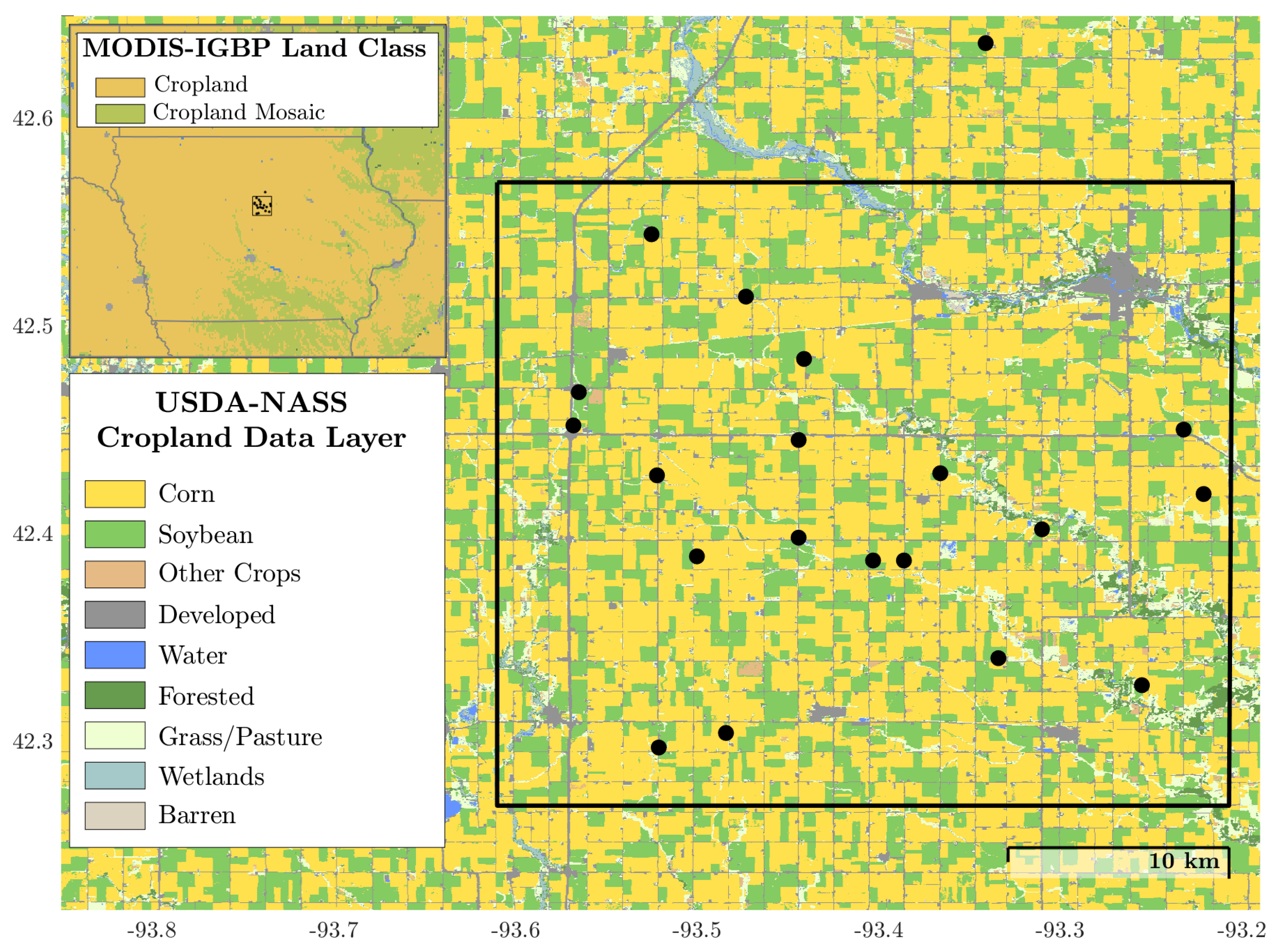
Figure 1 depicts the locations of the 20 permanent stations along with the corresponding SMAP EASE09 cell (row:264, col:928) and its 33 km radiometric resolution. The base map in Figure 1, the 2018 USDA National Agricultural Statistics Service (USDA NASS) Cropland Data Layer [18], illustrates the relative homogeneity of croplands (primarily corn and soybean) as opposed to forests, open water, and urban areas; the MODIS-IGBP [19] land cover classification used by SMAP is also provided. Agriculture in the South Fork is rainfed (no irrigation); the network has observed a mean precipitation of 880 mm year⁻¹ since installation.

Spatial variation of precipitation is the largest factor in South Fork soil moisture heterogeneity due to the relatively consistent soil texture and topography in the network [17]. Therefore, the network soil moisture, hereafter referred to as “South Fork WASM,” is defined as the weighted average of the 20 5-cm in situ soil moisture sensors. The Vornoi diagram (Thiessen polygon) used to produce South Fork WASM allows for weighting of soil moisture patterns, caused by spatial variation in rainfall events within the network that are observed by irregularly spaced stations. The installation of 20 stations provides some cushion for malfunctions; South Fork WASM does not differ significantly after approximately ten stations are considered [12]. In the event of missing data (i.e., a non-reporting station), the weights of missing stations are re-distributed across those remaining to dampen the impact of highly-weighted stations on calculated WASM.

Network stations are situated on the edges of fields, rather than within the crops, to avoid conflicts with farm management practices. In-field observations collected during summer 2014 to quantify the difference between soil moisture observed by the permanent stations and that of the adjacent fields in the South Fork found essentially no bias between the two; however, the RMSE was 0.023 m³ m⁻³ [12]. This indicates that some of the SMAP mission goals for random error (≤0.04 m³ m⁻³) currently have to be budgeted towards the South Fork in situ network itself. Future scaling schemes derived from the extensive in-field soil moisture sampling during the SMAPVEX16-IA campaign may reduce the impact of edge-of-field stations on the network. In addition, contributing to random error (but not the bias) are the differing sampling volumes between the South Fork in situ measurements at 5 cm and SMAP, which observes the top 3 to 6 cm of soil depending on moisture conditions [20].

Radio frequency interference (RFI), which increases observed $T_B$ and causes dry-biased L2SM retrievals, occurs when there is illegal broadcasting at L-band. Approximately 20% of SMAP overpasses in the South Fork have been flagged for further review by the RFI detection and mitigation algorithms in SMAP Level 1B processing since launch. Quality flags in the L2SM product indicate that >96% of the flagged $T_B$ subsequently pass mitigation, resulting in <1% of all SMAP overpasses in the South Fork being discarded due to RFI contamination. We therefore consider RFI to be negligible in the South Fork.

3. SMAP L2SM Performance in the South Fork

We evaluated SCA-H, SCA-V, and DCA SMAP L2SM retrievals (described in Section 2.2) monthly against South Fork WASM for April 2015–November 2018. The winter months (DJF) are excluded to avoid potentially including retrievals tainted by un-flagged snow or frozen soil.

Table 1. Bias between SMAP Level 2 Soil Moisture (L2SM) and South Fork weighted average soil moisture (WASM).

Single Channel Algorithm Applied to h-pol${\mathit{T}}_{\mathit{B}}$(SCA-H)

Bias, m3 m−3

Mar

Apr

May

Jun

Jul

Aug

Sep

Oct

Nov

All

a.m.

p.m.

2015

0.100

−0.100

−0.038

0.016

−0.010

−0.028

0.003

0.001

−0.094

−0.030

−0.037

−0.025

2016

−0.098

−0.083

0.002

−0.037

−0.013

−0.017

−0.015

−0.015

−0.084

−0.039

−0.044

−0.034

2017

−0.078

−0.056

−0.013

0.006

−0.005

0.019

−0.009

−0.037

−0.126

−0.030

−0.038

−0.022

2018

−0.085

−0.121

−0.051

0.049

−0.021

−0.017

0.005

−0.037

−0.090

−0.040

−0.049

−0.030

All Years

−0.087

−0.089

−0.025

0.007

−0.012

−0.010

−0.004

−0.022

−0.107

−0.035

−0.042

−0.028

Single Channel Algorithm Applied to v-pol ${\mathit{T}}_{\mathit{B}}$ (SCA-V)

Bias, m3 m−3

Mar

Apr

May

Jun

Jul

Aug

Sep

Oct

Nov

All

a.m.

p.m.

2015

−0.062

−0.021

0.018

−0.029

−0.021

0.002

0.029

−0.040

−0.014

−0.013

−0.016

2016

−0.050

−0.033

0.024

−0.036

−0.031

−0.017

−0.022

0.015

−0.030

−0.020

−0.020

−0.020

2017

−0.036

−0.017

0.004

−0.006

−0.009

0.022

0.017

−0.015

−0.047

−0.009

−0.009

−0.009

2018

−0.035

−0.078

−0.020

0.044

−0.029

−0.026

−0.020

−0.021

−0.088

−0.027

−0.030

−0.025

All Years

−0.041

−0.047

−0.003

0.004

−0.024

−0.011

−0.005

0.003

−0.049

−0.018

−0.018

−0.017

Dual Channel Algorithm (DCA)

Bias, m3 m−3

Mar

Apr

May

Jun

Jul

Aug

Sep

Oct

Nov

All

a.m.

p.m.

2015

0.003

0.004

−0.022

−0.043

−0.008

0.006

0.081

0.070

0.011

0.015

0.006

2016

0.040

0.050

0.051

−0.037

−0.044

−0.017

−0.026

0.065

0.080

0.017

0.025

0.010

2017

0.033

0.048

0.030

−0.027

−0.011

0.027

0.047

0.020

0.048

0.024

0.033

0.015

2018

0.061

−0.014

0.024

0.041

−0.033

−0.030

−0.039

0.005

−0.021

−0.002

0.002

−0.007

All Years

0.043

0.023

0.028

−0.012

−0.032

−0.007

−0.002

0.044

0.048

0.013

0.019

0.006

and

Table 2. Unbiased root-mean-square error (ubRMSE) between SMAP L2SM and South Fork WASM.

Single Channel Algorithm Applied to h-pol${\mathit{T}}_{\mathit{B}}$(SCA-H)
ubRMSE, m3 m−3	Mar	Apr	May	Jun	Jul	Aug	Sep	Oct	Nov	All	a.m.	p.m.
2015		0.024	0.046	0.067	0.026	0.026	0.041	0.051	0.041	0.058	0.056	0.058
2016	0.037	0.040	0.108	0.052	0.056	0.045	0.041	0.034	0.031	0.064	0.070	0.058
2017	0.037	0.027	0.078	0.103	0.058	0.037	0.037	0.032	0.027	0.065	0.063	0.067
2018	0.063	0.029	0.041	0.066	0.032	0.034	0.057	0.048	0.061	0.072	0.071	0.071
All Years	0.047	0.039	0.077	0.081	0.046	0.040	0.045	0.045	0.043	0.065	0.065	0.064
Single Channel Algorithm Applied to v–pol $T_B$ (SCA–V)
ubRMSE, m3 m−3	Mar	Apr	May	Jun	Jul	Aug	Sep	Oct	Nov	All	a.m.	p.m.
2015		0.025	0.040	0.075	0.020	0.027	0.034	0.039	0.035	0.039	0.054	0.044
2016	0.035	0.038	0.090	0.047	0.051	0.048	0.031	0.024	0.030	0.053	0.058	0.047
2017	0.037	0.026	0.070	0.065	0.053	0.025	0.022	0.021	0.020	0.047	0.049	0.044
2018	0.060	0.021	0.042	0.051	0.032	0.027	0.035	0.039	0.059	0.054	0.057	0.051
All Years	0.045	0.037	0.067	0.067	0.043	0.038	0.035	0.038	0.042	0.051	0.055	0.047
Dual Channel Algorithm (DCA)
ubRMSE, m3 m−3	Mar	Apr	May	Jun	Jul	Aug	Sep	Oct	Nov	All	a.m.	p.m.
2015		0.032	0.045	0.048	0.024	0.041	0.043	0.042	0.034	0.056	0.055	0.057
2016	0.039	0.042	0.076	0.046	0.055	0.057	0.034	0.027	0.041	0.067	0.068	0.065
2017	0.050	0.034	0.070	0.038	0.053	0.042	0.031	0.023	0.028	0.050	0.052	0.045
2018	0.067	0.030	0.050	0.055	0.040	0.040	0.041	0.039	0.074	0.059	0.058	0.060
All Years	0.054	0.044	0.064	0.056	0.047	0.050	0.051	0.046	0.058	0.059	0.060	0.058

provide the bias and ubRMSE calculated monthly for both individual years and the entire period; the March–November averages are additionally split into AM (descending) and PM (ascending) overpasses. Over the entire April 2015–November 2018 period, SMAP L2SM is dry-biased when using the SCA (bias: −0.035 m³ m⁻³ and −0.018 m³ m⁻³ for h- and v-pol, respectively) and wet-biased for the DCA (bias: 0.013 m³ m⁻³). The ubRMSE over this period exceeds the mission accuracy goal (0.065, 0.051 and 0.059 m³ m⁻³, for SCA-H, SCA-V, and DCA, respectively). There are, on average, 27 to 30 successful retrievals per month during April–October; March (≈23) and November (≈25) have fewer as some fail due to snow.

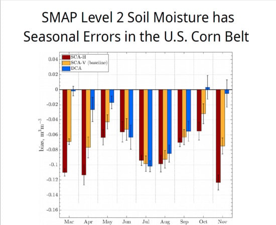
While the bias for the entire April 2015–November 2018 period is small (0.013 m³ m⁻³ (DCA); −0.035 m³ m⁻³ (SCA-H); −0.018 m³ m⁻³ (SCA-V)), there is both seasonal and inter-annual variation in the bias with individual monthly biases of ±0.10 m³ m⁻³. The SCA-H and SCA-V exhibit similar seasonal dynamics, with large dry biases (−0.04 to −0.10 m³ m⁻³) in early-spring and late-fall that improve to −0.02 m³ m⁻³ or better during the summer months when crops are present. The magnitude of the bias is typically larger for SCA-H than SCA-V. While the DCA is similar to the SCA during the summer months, it exhibits a moderate wet bias (0.02 to 0.04 m³ m⁻³) in the spring/fall when little to no vegetation is present.

The ubRMSE for both SCA, and to a lesser extent the DCA, peak in May/June (0.06 to 0.08 m³ m⁻³) when corn and soybean planting and emergence occur. There is also the most difference in ubRMSE between years at this time. These two months increase the overall ubRMSE; the remainder are near the SMAP mission accuracy goal of 0.04 m³ m⁻³. The SCA and DCA also have similar patterns when splitting ascending and descending overpasses; PM retrievals have a smaller bias magnitude, and to a lesser extent a lower ubRMSE, than AM retrievals.

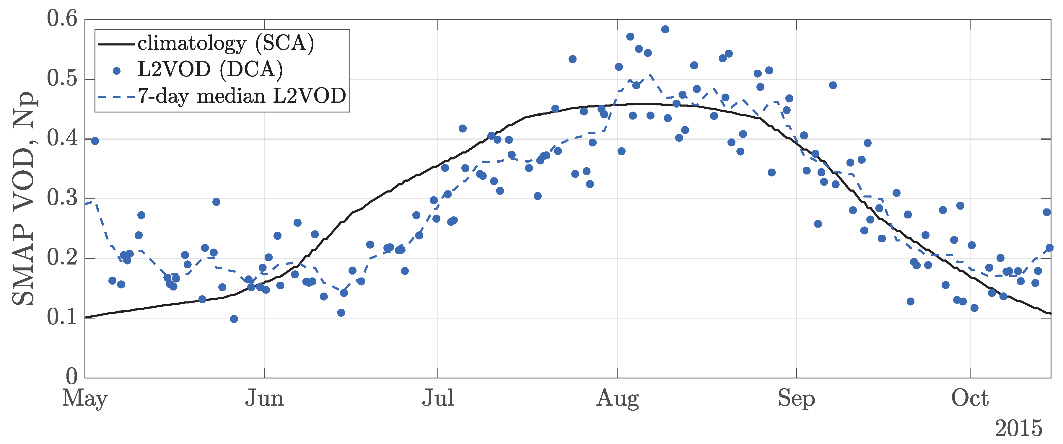
The differences between SCA and DCA bias and the large inter-annual variability in the transition between spring/fall and summer indicate that vegetation parameterization plays a major role in L2SM errors. In order to retrieve soil moisture, the $T_B$ measured by SMAP must be corrected for the effect of vegetation. This correction is made using a parameter called the vegetation optical depth (VOD) which characterizes attenuation of microwave radiation by vegetation. The times of largest ubRMSE correspond with the period when the climatological vegetation used by both SCA is potentially out-of-sync actual crop growth. SMOS Level 2 VOD (L2VOD), to which we assume SMAP L2VOD is similar, is proportional to corn and soybean development in the Corn Belt and therefore deviates from the climatological VOD due to annual variations in weather and farm management decisions [8]. Figure 2 presents a sample timeseries of the climatological VOD used by the SCA to correct for the effect of vegetation and the L2VOD retrieved by the DCA during soil moisture retrieval. During 2015, the sample year used for Figure 2, increases in climatological VOD preceded the corresponding L2VOD by more than two weeks during June and July. Section 5.1 addresses potential concerns for both the L2VOD and the climatological VOD as applied to the Corn Belt in more detail.

4. SMAP L2SM Algorithm

SMAP L2SM retrievals, regardless of SCA or DCA, are obtained by minimizing the difference between SMAP-observed $T_{B_p}$ and that simulated by the zeroth-order radiative transfer model commonly known as the $\tau -\omega$ model [21]. In addition to modelling bare soil, the $\tau -\omega$ model characterizes canopy emission and attenuation ($\tau$) as well as scattering by vegetation ($\omega$). $T_{B_p}$ is simulated in Equation (5) as the summation of radiation emitted from the soil and attenuated by the canopy (Equation 5a), radiation emitted upwards from the canopy (Equation 5b), and radiation emitted downwards from the canopy that reflects off the soil surface and travels back through the canopy (Equation 5c) [22,23,24]:

$$\begin{array}{cc}\hfill T_{B_p}=& T_{\mathrm{soil}}\left(1-R_{G_p}\right)\gamma \hfill \end{array}$$

(5a)

$$\begin{array}{cc}\hfill & +T_{\mathrm{veg}}(1-\omega )(1-\gamma )\hfill \end{array}$$

(5b)

$$\begin{array}{cc}\hfill & +T_{\mathrm{veg}}(1-\omega )(1-\gamma )R_{G_p}\gamma .\hfill \end{array}$$

(5c)

The assumption is made that, at SMAP overpass times, the soil temperature, $T_{\mathrm{soil}}$, and canopy temperature, $T_{\mathrm{veg}}$, are approximately the same and can be represented by an effective surface temperature, $T_{\mathrm{eff}}$ [21]. $T_{B_p}$ is modeled in Equations (6)–(10) as a function of: $T_{\mathrm{eff}}$; VOD, which is sometimes referred to as nadir $\tau$; incidence angle, $\theta$ (SMAP: $\theta$ = 40°); soil reflectivity, $R_{G_p}$; and the single scattering albedo, $\omega$. $R_{G_p}$ is a modification of the Fresnel reflectivity, $R_p$, itself dependent on the soil dielectric constant (relative permittivity), ${ϵ}_r$, to account for soil surface roughness and the angular sensitivity of roughness effects via the dimensionless coefficients HR and ${\mathrm{NR}}_p$. It is ${ϵ}_r$ that varies according to soil moisture: wet soil has an increased ${ϵ}_r$, and consequently a higher $R_p$ and smaller $T_{B_p}$, than a dry soil with the same physical characteristics:

$$\begin{array}{c}{T}_{B_p}=T_{\mathrm{eff}}\left[\gamma \left(1-R_{G_p}\right)+(1-\omega )(1-\gamma )\left(1+\gamma R_{G_p}\right)\right],\end{array}$$

(6)

$$\gamma =e^{-\mathrm{VOD}/cos\theta },$$

(7)

$$R_{G_p}=R_p{e}^{-\mathrm{HR}{(cos\theta )}^{{\mathrm{NR}}_p}},$$

(8)

$$R_h={\left|\frac{cos\theta -\sqrt{{ϵ}_r-{sin}^2\theta }}{cos\theta +\sqrt{{ϵ}_r-{sin}^2\theta }}\right|}^2,$$

(9)

$$R_v={\left|\frac{{ϵ}_{r}cos\theta -\sqrt{{ϵ}_r-{sin}^2\theta }}{{ϵ}_{r}cos\theta +\sqrt{{ϵ}_r-{sin}^2\theta }}\right|}^2.$$

(10)

In order for us to assess the impacts of varying surface parameterizations in SMAP L2SM, we must simulate L2SM. For each overpass, $T_{B_p}$ is simulated via Equations (6)–(10) for soil moisture between 0.02 m³ m⁻³ and porosity (constraints given by [14]). L2SM is then retrieved as the soil moisture that globally minimizes the cost functions given by Equation (11) or Equation (12) for the SCA or DCA, respectively. If the optimized $\Delta T_B$ exceeds 1.5 K, we consider the retrieval to be unsuccessful, and it is discarded. We are able to replicate SMAP L2SM SCA retrievals in the South Fork: the simulated SCA-H is 0.00018 ± 0.00009 m³ m⁻³ wetter than SMAP L2SM while the SCA-V is 0.00019 ± 0.00007 m³ m⁻³ drier. Our DCA replications are not as good as the SCA in accuracy and precision; the simulated DCA L2SM is 0.00065 ± 0.0002 m³ m⁻³ wetter than SMAP L2SM. Imperfect replications are likely due to differences in optimization (e.g., cost function, local vs global approach) between our simulations and the operational product:

$$\Delta T_{B_p}=|\mathrm{sim}{T}_{B_p}-\mathrm{obs}{T}_{B_p}|,$$

(11)

$$\Delta T_B=\sqrt{{\left(\Delta T_{B_h}\right)}^2+{\left(\Delta T_{B_v}\right)}^2}.$$

(12)

5. SMAP L2SM Parameterizations

We found that the SMAP L2SM bias and ubRMSE vary seasonally in the South Fork CVS. The bias exhibits distinct patterns dependent on the presence of vegetation while the ubRMSE peaks during the transition period between bare rough soil and annual crop growth. We hypothesize that incorrect treatment of parameters that vary seasonally in Equations (6)–(10) is the cause of observed errors. We therefore assessed the current parameterizations of: surface temperature and VOD; $\omega$ and soil surface roughness, which have the potential to change seasonally; and the static soil clay fraction. The following subsections present a discussion of each of these parameterizations as currently utilized for SMAP L2SM retrievals in croplands and their physical realism in the South Fork.

5.1. Vegetation Optical Depth (VOD)

SCA retrievals of SMAP L2SM are reliant on climatological vegetation optical depth (VOD). However, VOD varies intra- and inter-annually in agricultural regions such as the South Fork due to both farm management decisions that determine planting date (e.g., antecedent meteorological conditions, tillage practices, and cultivar [25]) and on temperature during crop development. This is due to corn and soybean development being governed by the accumulation of thermal time (e.g., [26]), a measure of daily average temperatures within the range hospitable to crop growth. There may additionally be long-term differences between VOD and the current climatology as multi-decadal analyses of crop phenology in the Corn Belt indicate that planting is occurring earlier and growing seasons are longer than they were thirty years ago [25,27].

As shown in Equations (5) and (7), $T_{B_p}$ increases as VOD increases (assuming no other changes). If climatological VOD is too low, as was the case during spring 2012 when significantly warmer than normal temperatures accelerated planting and emergence [28], then Equations (6)–(10) would retrieve a dry-biased soil moisture. Conversely, the use of a climatological VOD during a spring and early summer with delayed crop development would result in a wet bias during that period. This time corresponds with when SMAP L2SM SCA retrievals are noisiest in the South Fork.

The DCA attempts to bypass issues associated with climatological VOD by simultaneously retrieving L2SM and L2VOD. The sample timeseries of VOD previously given in Figure 2 illustrates how the timing of SMAP DCA-retrieved L2VOD, which presumably represents the “actual” VOD, can differ from the SCA climatology during a single year. While retrieval of L2VOD by SMAP is theoretically possible, if $T_{B_h}$ and $T_{B_v}$ are not fully independent, then there may not be enough information available when only a single incidence angle is sampled [29]. Furthermore, variations in soil surface roughness are interpreted by the DCA as L2VOD due to their producing the same changes to observed $T_{B_p}$ at L-band [30]. This is observed in the sample SMAP L2VOD timeseries in Figure 2, where VOD increases during the spring and fall despite the lack of significant vegetation. Limitations aside, L2VOD provides useful information about the status of crop progress. SMOS L2VOD, similar to SMAP but retrieved using a large range of observed $\theta$, peaks after having accumulated a thermal time of approximately 1000 °C·day post-planting in the U. S. Corn Belt [8]. This occurs between the second and third reproductive developmental stages of corn when $M_w$, defined as the mass of water in vegetation tissue per ground area, of the mixed corn and soybean canopy is at a maximum [8].

5.2. Effective Surface Temperature

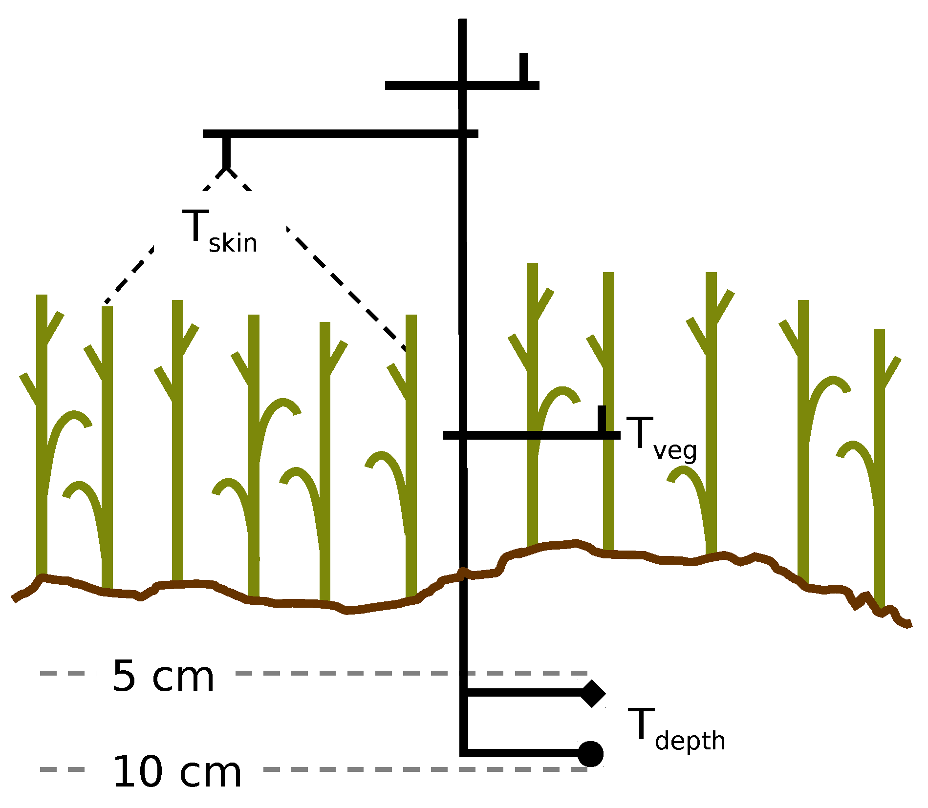
How realistic is the assumption that $T_{\mathrm{soil}}\approx T_{\mathrm{veg}}$ at SMAP overpass times? This assumption is made so that $T_{\mathrm{eff}}$, dependent only on soil temperature, can be used to approximate the temperature of the entire surface viewed by SMAP. We compared flux tower observations of soil and vegetation temperatures at a central location in the South Fork for both corn (2015, 2018) and soybean (2015). Sampling was provided by Forrest Goodman (USDA, National Laboratory for Agriculture and the Environment) in 2015 and by Richard Cirone (Iowa State University, Department of Agronomy) in 2018. Figure 3 illustrates relevant temperature observations. In addition to the more traditional infrared skin temperature, $T_{\mathrm{skin}}$, the air temperature within the canopy, $T_{\mathrm{veg}}$, was observed. Vertical temperature gradients in fully-grown corn are ≈1 K [31]; this is accounted for in $T_{\mathrm{veg}}$ sampling by vertically centering the observation within the canopy. As such, observations of $T_{\mathrm{veg}}$ are limited to closed canopy periods (June–September). Soil temperature, $T_{\mathrm{depth}}$, was sampled at 6 cm in 2015 and 9 cm in 2018.

Table 3. Difference between vegetation canopy temperature, $T_{\mathrm{veg}}$, and soil temperature, $T_{\mathrm{depth}}$, in corn and soybean, where $T_{\mathrm{depth}}$ is 6 cm in 2015 and 9 cm in 2018 as illustrated in Figure 3. Data is limited to SMAP overpass times in June–September.

${\mathbf{T}}_{\mathbf{veg}}$ – ${\mathbf{T}}_{\mathbf{depth}}$, K
	Corn		Soybean
	a.m.	p.m.	a.m.	p.m.
6 cm (2015)	−2.1	2.3	−1.9	0.6
9 cm (2018)	−2.5	1.7

presents the difference between $T_{\mathrm{veg}}$ and $T_{\mathrm{depth}}$ in corn and soybean for SMAP retrievals in June–September. For both crop types, $T_{\mathrm{veg}}$ averages colder than $T_{\mathrm{depth}}$ for morning overpasses and warmer for evening. This is consistent with previous investigation of vertical temperature gradients in a corn field that found the canopy was, on average, 2.5 K colder than the 4.5 cm soil temperature (shallower than $T_{\mathrm{depth}}$) at 6:00 a.m. solar time and 0.75 K warmer at 6:00 p.m. solar time [31]. The 2015 comparison of $T_{\mathrm{veg}}$ and $T_{\mathrm{depth}}$ shows a slightly smaller difference (less negative) for morning overpasses and a larger (warmer) difference in the evening than observed in 2018; this is due to the discontinuity in installation depth. The deeper you observe soil temperature, the more diurnal variations are dampened from those of the soil surface [32]. The 2015 $T_{\mathrm{depth}}$, inserted at 6 cm, is therefore cooler for morning overpasses and warmer in the evening as compared to the deeper 9 cm sampling of 2018.

While $T_{\mathrm{soil}}\not\approx T_{\mathrm{veg}}$ at SMAP overpass times in the South Fork, recall that $T_{\mathrm{eff}}$ is meant to represent the combined effect of the two temperatures on $T_{B_p}$. $T_{\mathrm{eff}}$ is defined by Equation (13) via a modified Choudhury model [33] as a function of the GEOS-5 0 to 10 cm and 10 to 30 cm layer temperatures ($T_{\mathrm{SL}1}$ and $T_{\mathrm{SL}2}$, respectively), a coefficient, C, that weights the relative contributions of $T_{\mathrm{SL}1}$ and $T_{\mathrm{SL}2}$, and a bias correction factor, K [34]. $T_{\mathrm{eff}}$ is reported for each SMAP overpass in the SPL2SMP_E product:

$$T_{\mathrm{eff}}\triangleq K\left[T_{\mathrm{SL}2}+C\left(T_{\mathrm{SL}1}-T_{\mathrm{SL}2}\right)\right].$$

(13)

In version 2 of the SPL2SMP_E (CRID: R16xxx), $K=1.02$ for non-forest land classes, $C=0.246$ for morning overpasses, and $C=1$ for evening overpasses [34]. At the beginning of the SMAP mission, K was not a component of Equation (13) (equivalently $K=1$) and $C=0.246$ for all L2SM retrievals [21]. $K=1.02$, which warms $T_{\mathrm{eff}}$, was prompted by an observed cold bias in the GEOS-5 soil temperature at CVSs. It is also intended to address any potential mismatch between the GEOS-5 modeled soil layers and the layer of soil contributing to the temperature of the surface that SMAP views. Again, while calculated using modeled soil layer temperatures, $T_{\mathrm{eff}}$ is not a physical soil temperature and is intended to represent both the vegetation canopy and the soil layer observed by the SMAP radiometer. The value of $K=1.02$ for non-forest land classes was derived by minimizing the difference between the baseline $T_{B_v}$ and that simulated via the SCA-V (personal communication, Steven Chan, NASA Jet Propulsion Laboratory).

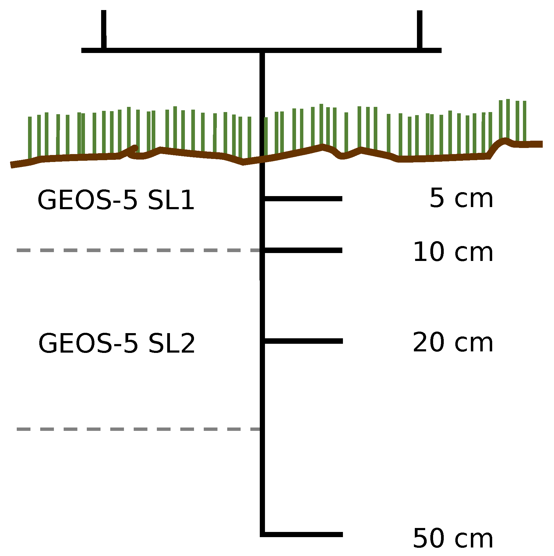
The difference between SMAP $T_{\mathrm{eff}}$ and “network $T_{\mathrm{eff}}$,” as well as the differences between SMAP $T_{\mathrm{eff}}$ and observed in situ depths, are presented in

Table 4. Difference between SMAP $T_{\mathrm{eff}}$ and South Fork soil temperature for April 2015–November 2017 (excluding DJF).

SMAP ${\mathbf{T}}_{\mathbf{eff}}$ —South Fork In Situ Temperature, K
	SPL2SMP_E, v1		SPL2SMP_E, v2		Proposed ${\mathit{T}}_{\mathrm{eff}}$
	$\mathit{K}=\mathbf{1}$		$\mathit{K}=\mathbf{1.02}$		$\mathit{K}=\mathbf{1}$
	$\mathit{C}=\mathbf{0.246}$	$\mathit{C}=\mathbf{0.246}$	$\mathit{C}=\mathbf{0.246}$	$\mathit{C}=\mathbf{1}$	$\mathit{C}=\mathbf{0.246}$	$\mathit{C}=\mathbf{1}$
	a.m.	p.m.	a.m.	p.m.	a.m.	p.m.
network $T_{\mathrm{eff}}$	−1.1	−0.7	−1.2	0.6	−1.2	0.6
5 cm	−0.7	−1.7	5.0	6.4	−0.7	0.6
10 cm	−0.9	−1.3	4.8	6.9	−0.9	1.1
20 cm	−1.3	−0.3	4.4	7.8	−1.3	2.0
50 cm	−1.1	0.6	4.6	8.7	−1.1	2.9

. Network $T_{\mathrm{eff}}$ is calculated using Equation (13) and South Fork in situ measurements, where $T_{\mathrm{SL}1}$ is the soil temperature at a depth of 5 cm, $T_{\mathrm{SL}2}$ is the temperature at 20 cm, and both K and C are parameterized as given in Table 4. The correspondence between GEOS-5 temperatures (and thus $T_{\mathrm{SL}1}$ and $T_{\mathrm{SL}2}$) and South Fork in situ soil temperatures is shown in Figure 4. The period was limited to April 2015–November 2017 (excluding DJF) as 2017 is the last full year of SPL2SMP_E version 1 retrievals.

In version 1 of the SPL2SMP_E (CRID: R14xxx–R15xxx), when K was not a part of $T_{\mathrm{eff}}$ calculation, the difference between SMAP $T_{\mathrm{eff}}$ (computed using GEOS-5 temperatures) and network $T_{\mathrm{eff}}$ in Table 4 is similar to the difference between SMAP $T_{\mathrm{eff}}$ and the raw in situ measurements at 5, 10, 20, and 50 cm: all are within ±2 K. In version 2 of the SPL2SMP_E (CRID: R16xxx), SMAP $T_{\mathrm{eff}}$ (computed using GEOS-5 temperatures) is much warmer than the raw in situ measurements at 5, 10, 20, and 50 cm (by 4 to 9K). This could only be realistic for the combined soil-vegetation surface if $T_{\mathrm{veg}}$ was significantly hotter (by at least 10 K) than $T_{\mathrm{soil}}$. This is contrary to our flux tower observations that show $T_{\mathrm{veg}}<T_{\mathrm{soil}}$ for morning overpasses and $T_{\mathrm{veg}}$ only 1 to 2 K warmer than $T_{\mathrm{soil}}$ for evening overpasses. Evening overpasses were warmed more in version 2 as the use of $C=1$ results in $T_{\mathrm{eff}}$ being calculated entirely based on $T_{\mathrm{SL}1}$ rather than weighting towards $T_{\mathrm{SL}2}$ as with $C=0.246$.

We propose a modification to $T_{\mathrm{eff}}$ that is more consistent with in situ network soil temperatures and would better approximate the differences between $T_{\mathrm{veg}}$ and $T_{\mathrm{soil}}$ at SMAP overpass times. This can be done by reverting to $K=1$ (i.e., reversing the SPL2SMP_E adoption of $K=1.02$) but retaining the SPL2SMP_E version 2 change to $C=1$ for evening overpasses. The cold bias in $T_{\mathrm{eff}}$ that would return when $K=1$ has a similar numerical effect of a colder morning canopy on surface temperature. While this would also make evening $T_{\mathrm{eff}}$ colder, utilizing $C=1$ in Equation (13) weights $T_{\mathrm{eff}}$ towards the warmer evening $T_{\mathrm{SL}1}$. The difference between our proposed $T_{\mathrm{eff}}$ and both the network $T_{\mathrm{eff}}$ and observed in situ depths is shown in column three of Table 4. As desired, SMAP $T_{\mathrm{eff}}$ (which should account for the effect of both soil and vegetation temperatures) is about 1 K cooler than the network $T_{\mathrm{eff}}$ (computed using only soil temperatures) at the AM overpass, and about 1 K warmer at the PM overpass. This method requires only the ancillary data already provided in the SPL2SMP_E. It is most applicable to overpasses that occur during vegetated periods. A truly representative approach may be to utilize separate $T_{\mathrm{veg}}$ and $T_{\mathrm{soil}}$ during L2SM retrieval, where $T_{\mathrm{veg}}$ could be approximated by the GEOS-5 $T_{\mathrm{surf}}$, which was a component of $T_{\mathrm{eff}}$ calculation prior to launch [21], and $T_{\mathrm{soil}}=T_{\mathrm{eff}}$.

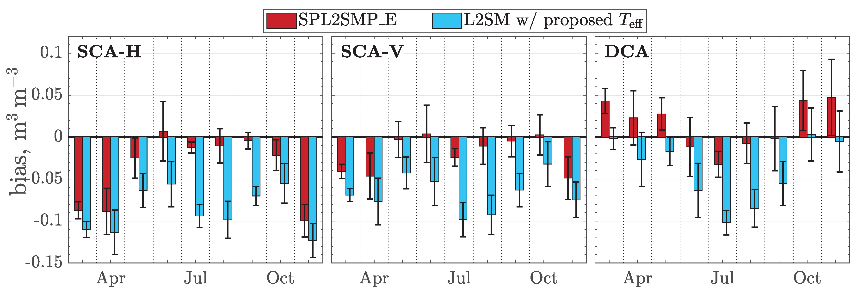
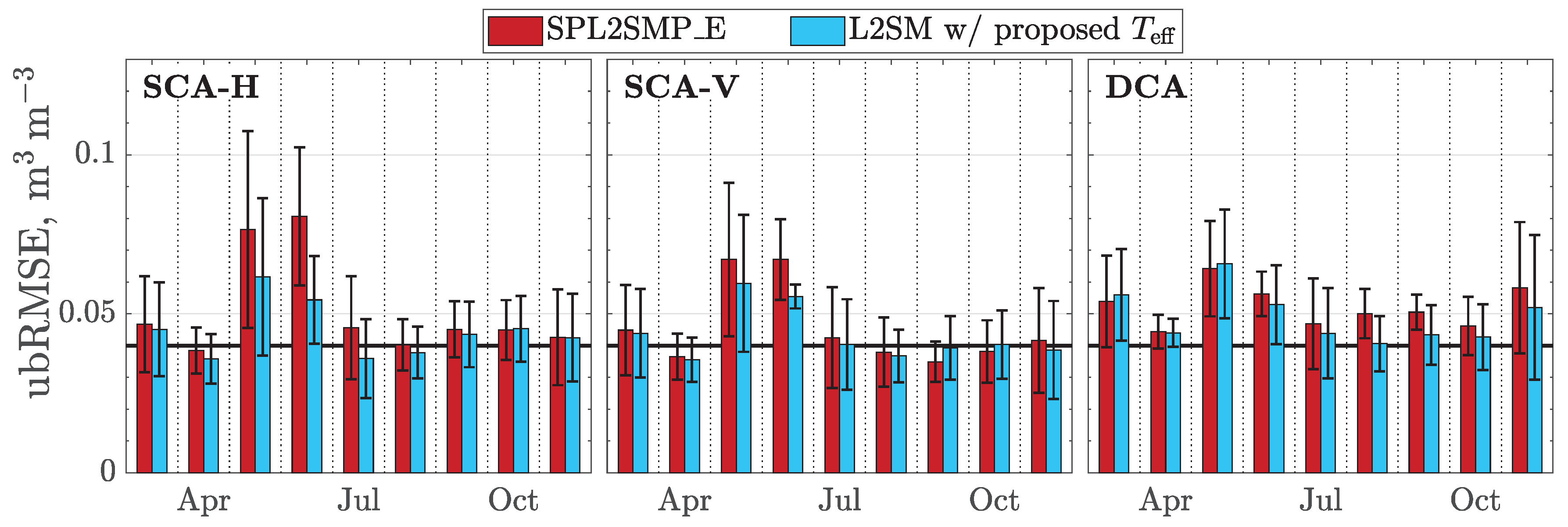
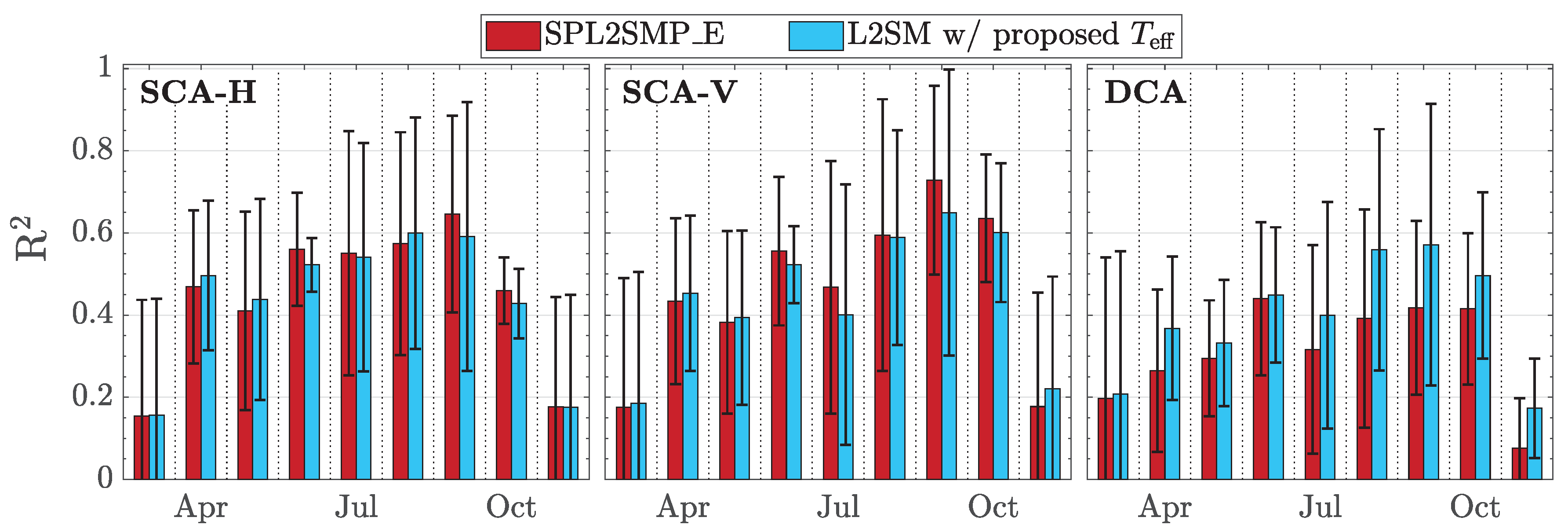
Figure 5, Figure 6 and Figure 7 present the effect of adopting the more realistic modified $T_{\mathrm{eff}}$ in the South Fork as quantified by the bias, ubRMSE, and R², respectively. Decreasing $T_{\mathrm{eff}}$ dries monthly biases for both SCA and the DCA: mean SCA retrievals are at least 0.03 and as much as 0.12 m³ m⁻³ too low as compared to in situ South Fork measurements, and DCA retrievals vary from about zero bias in the fall and early spring to 0.10 m³ m⁻³ too low in the middle of the summer. This occurs because the retrieval algorithms now calculate a higher ${ϵ}_r$ for the same observed $T_B$. While this is worse performance in terms of bias, the monthly ubRMSE decreases, particularly for both SCA in May/June when they previously far exceeded the SMAP mission accuracy goal. This is likely due to $K=1.02$ amplifying any noisiness in GEOS-5 temperatures by an additional 2%. The coefficient of determination significantly improves for the DCA (its mean value is higher in every month) when the modified $T_{\mathrm{eff}}$ is used; however, large inter-annual variations remain for all three algorithms. R² does decrease slightly for the SCA when the modified $T_{\mathrm{eff}}$ is used during retrieval; however, this is not surprising when you consider that the $K=1.02$ depth correction scheme was intended to optimize $T_{B_v}$.

The significant difference between $T_{\mathrm{eff}}$ and observed temperatures at all in situ depths leads to the conclusion that $K=1.02$ does not produce a physically realistic surface temperature. Flux tower observations of soil temperature and $T_{\mathrm{veg}}$ indicate that using $K=1$ to calculate $T_{\mathrm{eff}}$, in conjunction with using $C=1$ for evening overpasses and the slight cold bias of GEOS-5 soil temperature in the South Fork, reproduces the effect of having a cooler canopy in the morning but a warmer canopy in the evening. While retrieving L2SM with the modified $T_{\mathrm{eff}}$ does degrade the bias in the South Fork, the combination of improved ubRMSE for both SCA and DCA and the significantly increased coefficient of determination for DCA can be interpreted as an overall improvement in retrieval quality if we consider that the bias may be caused by some other ancillary factor.

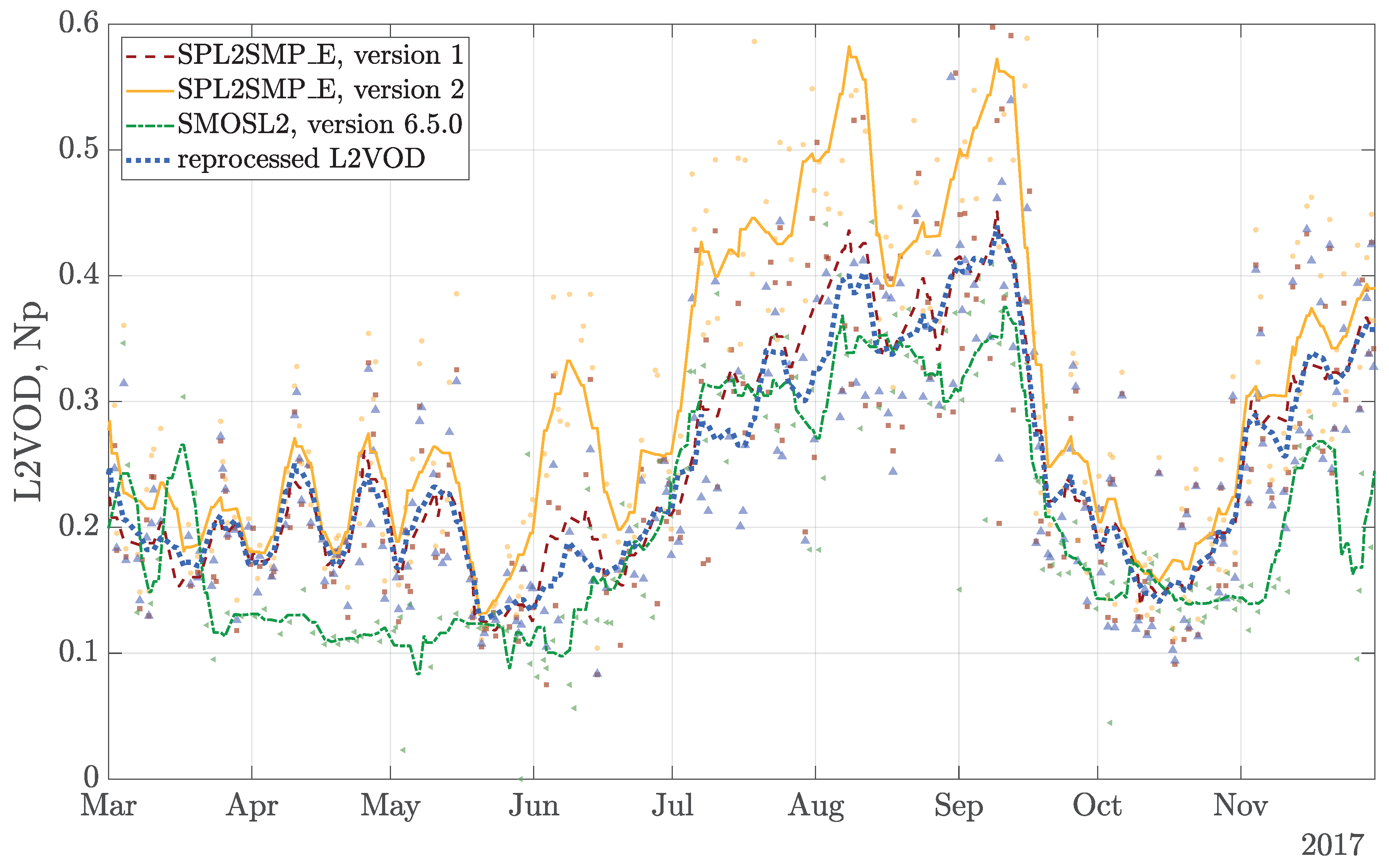
An additional consideration of modifying $T_{\mathrm{eff}}$ is how it affects retrieved L2VOD. The VOD produced during our DCA retrievals using the proposed $T_{\mathrm{eff}}$ will hereafter be referred to as “reprocessed L2VOD.” Figure 8 presents a comparison of L2VOD in the South Fork during 2017 as retrieved by both versions 1 and 2 of the SPL2SMP_E product, the reprocessed L2VOD, and VOD from SMOS. When $T_{\mathrm{eff}}$ was warmed dramatically in version 2 of the the SPL2SMP_E, the DCA-retrieved L2VOD increased with it. This was problematic for those utilizing the vegetation product as the operational L2VOD is now unrealistically large. L2VOD retrieved using our $T_{\mathrm{eff}}$ decreases back to values similar to those of the version 1 SPL2SMP_E and is in-line with the SMOS L2VOD in the South Fork. The L2SM and L2VOD reprocessed with our modified $T_{\mathrm{eff}}$ are publicly available for EASE09 pixels in the state of Iowa as Supplementary Material.

5.3. Single Scattering Albedo

Scatter darkening, where $T_{B_p}$ is reduced by radiation scattering within the canopy, occurs when the size of plant components (e.g., stems, leaves, ears) is similar to the wavelength (SMAP: $\lambda =$ 21 cm). This effect must be considered in corn [35,36]. The components of soybean plants are much smaller and as such there is relatively little scattering [36]. The $\tau -\omega$ model, which assumes that the canopy is a weakly scattering media, accounts for this via the $\omega$ parameter [37]. Non-zero values of $\omega$ inform Equations (6)–(10) that $T_{\mathrm{eff}}$, and hence $T_{B_p}$, has been reduced by scattering.

The South Fork CVS is classified as entirely croplands by the MODIS-IGBP [3] and consequently $\omega$ is parameterized as 0.05 [21]. While $\omega =0.05$ for SMAP, there have been several values of $\omega$ used for L-band soil moisture retrieval in croplands. For example, while noting that certain crop types, such as corn, can approach $\omega =0.10$, the SMOS L2 algorithm treats all “low vegetation” such as croplands to be non-scattering ($\omega =0$) [38]. The SMOS-IC algorithm parameterizes stronger scattering ($\omega =0.12$) [39]. The MT-DCA utilizes an $\omega$ retrieved from SMAP $T_{B_p}$ timeseries; 0.04 ± 0.04 for croplands pixels [40]. We simulated L2SM using $\omega =$ 0, 0.05 and 0.12 for the South Fork CVS to determine the effect changing $\omega$ has on retrieval performance. $T_{\mathrm{eff}}$ was calculated via our more physically realistic proposed method (Section 5.2). The resulting metrics are given in

Table 5. L2SM metrics in the South Fork for $\omega$ = 0, 0.05 and 0.12 during June–September, 2015–2018.

	Bias, m3 m−3			ubRMSE, m3 m−3			R2
	SCA-H	SCA-V	DCA	SCA-H	SCA-V	DCA	SCA-H	SCA-V	DCA
$\omega =0$	0.009	−0.004	−0.014	0.059	0.046	0.061	0.54	0.55	0.27
$\omega =0.05$	−0.044	−0.064	−0.077	0.053	0.055	0.051	0.54	0.50	0.48
$\omega =0.12$	−0.098	−0.119	−0.126	0.078	0.107	0.079	0.30	0.09	0.28

for a crop development subset of June–September, 2015–2018.

The June–September, 2015–2018 bias is smallest when $\omega =0$. The SCA-V additionally has the least amount of noise and is more correlated when $\omega$ is small. The SMAP default for croplands, $\omega =0.05$, results in drier soil moisture retrievals; however, this is more physically realistic than parameterizing the annual crops as non-scattering. DCA performance in terms of ubRMSE and R² significantly improves with the increase to $\omega$. Retrieving SMAP L2SM utilizing $\omega =0.12$ for croplands, as is done in the SMOS-IC algorithm, worsens the dry bias and significantly degrades ubRMSE and R². In addition, using a larger value of $\omega$ reduces the number of soil moisture retrievals. Only 42% (201 of 479 overpasses) of attempted SCA-V retrievals with $\omega =0.12$ are successful during June–September, 2015–2018, while 91% (435 of 479) of attempted SCA-V retrievals are successful when $\omega =0$. The SCA-H and DCA were both better able to optimize $T_B$ at $\omega =0.12$ with 83% (361 of 479) of attempted retrievals being successful. Our attempted retrievals fail when the difference between simulated and observed $T_B$ in the cost functions given by Equation (11) and Equation (12) is >1.5 K.

The difference between SCA-V and SCA-H behavior suggests that scattering effects in the South Fork are lesser for v-pol than h-pol. While $\omega$ is often assumed to be unpolarized [41], several tower-based experiments have found that ${\omega }_h\ne {\omega }_v$ in agriculture. This would occur if scattering plant structures appeared different when observed at h– and v–pol; for example, ${\omega }_h>{\omega }_v$ for the REBEX-8x experiment in corn [35]. Table 5 indicates that lower values of $\omega$ result in the best soil moisture retrievals as quantified by ubRMSE and R².

5.4. Soil Texture

In soil, water molecules can either be mobile (free water) or tightly bound to the surface area of particles (bound water) [42]. Bound water exhibits distinctly different dielectric properties than free water at L-band [43]. The amount of bound water is determined by soil texture as characterized by particle size distribution: the largest particles are sand (2 to 0.05 mm), the smallest are clay (<0.002 mm), and those in between are silt. A predominantly clay soil has a much larger particle surface area, and consequently more bound water, than a sandy soil. Inaccuracies in parameterized clay fraction therefore result in errors in retrieved soil moisture as the bound water component is miscalculated. Overestimation of clay theoretically results in wet-biased retrievals as the algorithms add more bound water when calculating ${ϵ}_r$ for high clay soils.

Dielectric mixing models simulate ${ϵ}_r$, the component of Equations (6)–(10) that allows for soil moisture retrieval, as a function of soil moisture, texture, and temperature. SMAP L2SM is currently retrieved using the Mironov model [44], although functionality exists for both the Dobson [45] and Wang and Schmugge [46] models to be implemented if desired [34]. Utilizing the Mironov model, which requires ancillary soil temperature and clay fraction, results in wetter global soil moisture retrievals than the Dobson model [47]. The Dobson and Wang and Schmugge models additionally require sand fraction and bulk density.

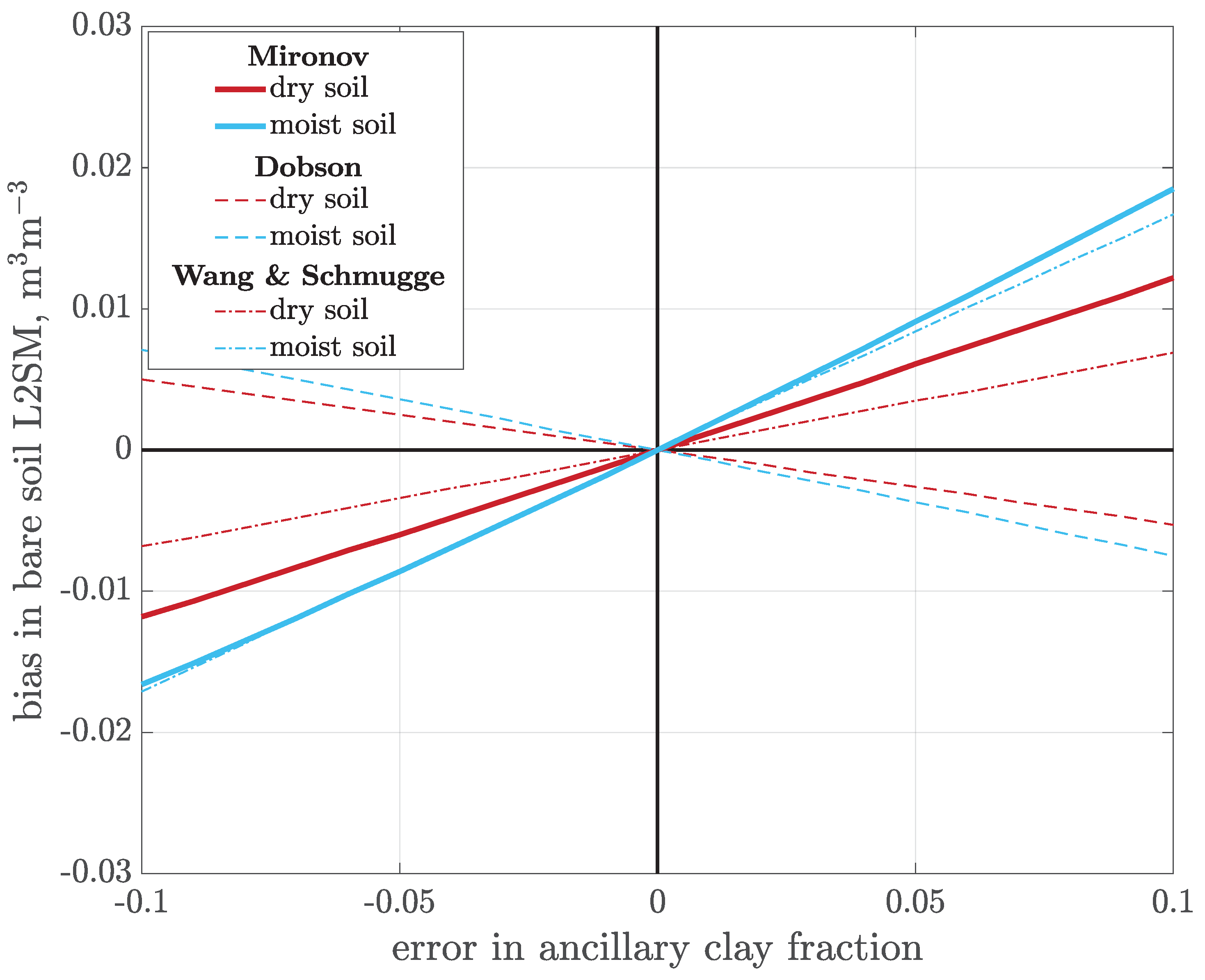
Figure 9 presents the sensitivity of L2SM retrieval to errors in the SMAP ancillary clay fraction for a bare soil scenario (VOD = 0) with clay fractions within ±0.10 of the SMAP L1-L3 Ancillary Static Data value of 0.31 in the South Fork. Moderately moist to saturated soils (tested: 0.25 and 0.40 m³ m⁻³) have similar sensitivities while dry soils (tested: 0.10 m³ m⁻³) are less sensitive. This is due to there being two distinct regions in ${ϵ}_r$ sensitivity to soil moisture that are separated by a “transition soil moisture” related to the wilting point [46]. The Dobson and Wang and Schmugge models are included in Figure 9 to illustrate how changing the dielectric model used during L2SM retrieval would affect the sensitivity to clay for a soil whose sand fraction and bulk density are similar to that of the South Fork. While both the Mironov and Wang and Schmugge models both behave as expected, with overestimation of clay content resulting in wet-biased retrievals as theorized, the Dobson model exhibits an inverse relationship. This was previously noted for South Fork soil textures and is likely due to the empirical nature of dielectric mixing models [12]. We tested soil temperatures of 280, 290 and 300 K (Figure 9 was produced for 300 K); temperature was not found to have a significant impact on the L2SM sensitivity to clay fraction within this range.

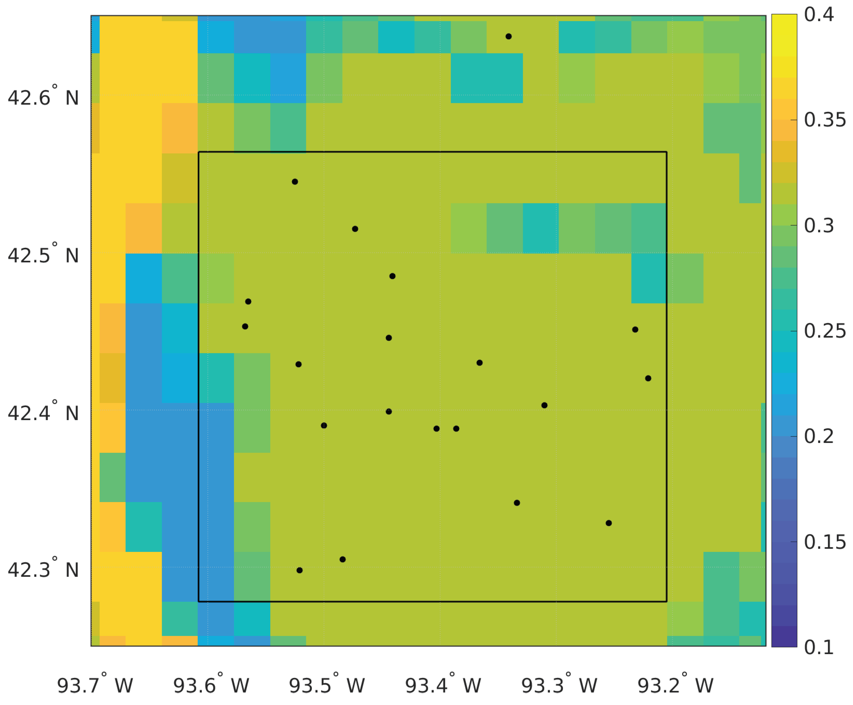
The SMAP ancillary clay fraction is derived from STATSGO, the State Soil Geographic dataset [48], over CONUS and posted to the EASE03 [49]. Figure 10 provides a subset of this map for the South Fork. The 33 km radiometric domain for EASE09 cell [row:264, col:928] and the in situ stations presented in Figure 1 are overlaid for reference. While SMAP L2SM is posted to the EASE09 grid, the clay fraction utilized during retrieval is that of the radiometric domain (personal communication, Narendra Das, NASA JPL). The SMAP clay fraction for the 33 km domain over the South Fork is 0.31. The Soil Survey Geographic Database (SSURGO), which has a finer scale than STATSGO (100 to 500 m vs 2.5 km), indicates a clay fraction of 0.27 for the South Fork (personal communication, Alex White, USDA ARS Hydrology and Remote Sensing Laboratory). The SSURGO value of 0.27 has been used in previous modeling of the South Fork CVS [17]. If the “true” clay fraction in the South Fork is similar to the SSURGO value, then Figure 9 suggests that SMAP L2SM retrievals for bare soil may currently be 0.004 to 0.007 m³ m⁻³ wetter than they should be. The impact would be lesser for vegetated periods. Interestingly, while the SMOS mission utilizes the same ancillary dataset as SMAP, albeit posted to different grid with ≈4 km resolution [50], the clay fraction of its map is 0.25 for the South Fork domain [12], which is closer to that derived from SSURGO.

5.5. Soil Surface Roughness

Soil surface roughness, defined as mm-scale variations in soil surface height, is rarely smooth in agricultural fields and is dependent on field management activities such as tillage [51]. This is particularly important when modelling $T_{B_p}$ as a rough soil is less reflective, and thus has a higher emissivity, than a smooth soil with the same characteristics [52,53]. Roughness additionally effects the L-band sampling depth as smooth soils have a shallower sampling depth than equivalent rough soils during dry conditions [54]. SMAP L2SM retrievals account for roughness in Equation (8) as an exponential decay of the specular reflectivity, $R_p$, characterized by non-dimensional coefficients HR and NR${}_p$; for croplands, HR = 0.108 [21] and ${\mathrm{NR}}_p=$ 2 for both h- and v-pol [34].

Tillage, prevalent in the South Fork [55], increases soil surface roughness as residue (dead plant material) from the prior crop is churned into the upper layer of soil. If the South Fork soils are, on average, rougher than the relatively smooth soil parameterized, then SMAP L2SM would be biased dry, particularly during periods of bare soil. This correlates with observed dry biases for both the SCA-H and SCA-V; however, the DCA does not exhibit a dry bias during the bare soil period (March–May and October–November). That said, the DCA-retrieved SMAP L2VOD is likely masking the effect of a too-smooth soil parameterization. Changes in soil surface roughness appear the same at L-band as changes in L2VOD [30]. Therefore, when HR is assumed to be static, as is the case in SMAP L2SM retrieval, any increase to surface roughness is interpreted by the DCA as increasing vegetation. This is visible in the sample L2VOD timeseries, previously given in Figure 2 and Figure 8, where L2VOD is unrealistically large during the non-vegetative spring and late-fall months and subsequently wets L2SM retrievals similar to how assuming a rougher soil would.

L-band retrievals of soil moisture are especially sensitive to parameterization of roughness [41]. There are several methods to convert physical observations (e.g., standard deviation of soil surface height) to the non-dimensional HR [41,52,56]. Attempts to retrieve HR directly, either from tower-based or satellite observations of $T_{B_p}$, have produced variable results with HR ranging from near 0 to <2 for bare soil and cultivated croplands ([56,57,58,59] and others). SMAP documentation does not recommend a particular method for calculating HR.

6. Summary

Seasonal analysis of SMAP L2SM performance in the South Fork reveals that patterns in the bias, for both SCA and DCA, follow distinct periods of bare soil (spring and fall) and annual crop development (summer). The ubRMSE is worst during May/June when crops emerge and rapidly begin to obscure the soil surface. We evaluated the parameterizations of $T_{\mathrm{eff}}$, VOD, $\omega$, clay fraction, and soil surface roughness to determine if they are physically realistic for the South Fork. The main results are as follows:

• The $T_{\mathrm{eff}}$ used in version 2 of the SPL2SMP_E is 4 to 9 K warmer than any observed soil depth in the South Fork. Using $K=1$ to calculate $T_{\mathrm{eff}}$ is more physically realistic.
• The assumption that $T_{soil}$ and $T_{veg}$ is equivalent at SMAP overpass times is not valid in corn and soybean canopies; however, the overall impact on $T_B$ can be mitigated during $T_{\mathrm{eff}}$ calculation.
• Climatological VOD cannot reliably describe vegetation growth in the Corn Belt.
• Increasing $\omega$ to account for scattering in corn dries L2SM retrievals, worsening observed dry biases in SMAP L2SM during the summer months.
• The current clay fraction may be slightly over-estimated, but its impact on SMAP L2SM retrieval is minimal.
• Observed SMAP L2SM biases support the idea that the current HR is too smooth for the South Fork, consistent with the tillage practices of the region.

Table 6. Current understanding of SMAP soil moisture retrieval issues in the U.S. Corn Belt.

Issue	Understanding	Next Steps and Importance
radio-frequency interference (RFI)	RFI is minimal in most, if not all, of the Corn Belt (this work and [12]).	Continue to use RFI mitigation techniques (minor impact).
in situ soil moisture network representativeness (upscaling)	The 20 South Fork CVS stations are adequate for pixel characterization since as few as 5 indicate a SMAP dry bias [12].	Continue to improve station weighting function (moderate impact).
effective temperature $T_{\mathrm{eff}}$ in retrieval algorithm	$T_{\mathrm{eff}}$ in L2SM version 2 is 5–9 K too high as compared to in situ soil temperature (this work).	Use version 1 $T_{\mathrm{eff}}$ (major impact).
soil–vegetation canopy temperature gradient	$T_{\mathrm{soil}}\ne T_{\mathrm{veg}}$ at 6 a.m. and 6 p.m. (this work and [31]).	Consider separate $T_{\mathrm{soil}}$ and $T_{\mathrm{veg}}$ in retrieval algorithm or a modified $T_{\mathrm{eff}}$ (moderate impact).
sampling depth mismatch	Soil layer SMAP “sees” is different than what is observed by in situ sensors, which increases ubRMSE but not bias [20].	Take into account when assessing validation statistics (minor impact).
clay fraction	Different values used for South Fork CVS: STATSGO = 0.31; SSURGO = 0.27; SMOS = 0.25 (this work).	Resolve differences (minor impact).
soil dielectric model	Mironov [44] and Wang & Schmugge [46] models result in dry biased retrievals if clay is underestimated. Dobson model [45] exhibits the opposite behavior (this work and [12]).	Resolve differences (minor impact).
soil surface roughness	Soil roughness is not static: rainfall, tillage, and other soil management activities modify soil roughness throughout the year [30,51]. Roughness effect depends on soil moisture [56].	Use the DCA and allow roughness parameter HR to vary during bare-soil periods (major impact).
single-scattering albedo of vegetation canopy	Vegetation canopy volume scattering is significant [35]; non-zero values of $\omega$ increase dry bias, lower values of $\omega$ result in lower ubRMSE and higher R2 (this work).	Determine a satellite-scale $\omega$, consider how it may change with crop phenology (major impact).
vegetation optical depth	VOD varies from year-to-year due to weather and farm management activities [8].	Use the DCA and allow VOD to vary when crops are present (major impact).
vegetation transmissivity	Sensitivity to soil moisture is likely higher than predicted by current retrieval model [31]; allowing multiple scattering in vegetation canopy would reduce dry bias (this work and [60]).	Use a new radiometric forward model in the retrieval algorithm (major impact).

summarizes our current understanding of SMAP soil moisture retrieval issues in the Corn Belt, and suggests the next steps.

7. Conclusions

We hypothesized that a seasonal analysis of SMAP L2SM retrievals, rather than the annual analysis performed by prior investigations, is more appropriate for the South Fork Core Validation Site in the U.S. Corn Belt as there are two distinct land cover periods: annual crops in the summer and bare soil in the spring and fall. The overall annual bias, as compared to the South Fork in situ soil moisture network, is −0.018 m³ m⁻³ (retrievals are too dry) for the current baseline algorithm (SCA-V SMAP-L2SM version 2). However, individual monthly biases for the three retrieval algorithms approach or exceed ±0.10 m³ m⁻³, and there is a clear seasonal pattern in the validation metrics. The two single-channel retrieval algorithms (SCA-V and SCA-H) are exceptionally dry during the spring and fall months, become less biased near emergence and harvest, and are dry again during the summer when vegetation is present. The dual-channel algorithm (DCA), which utilizes both polarizations of observed brightness temperature, performs similarly during the summer but produces retrievals slightly wetter than the in situ network during bare soil periods. The seasonal behavior of DCA performance is similar to that of SMOS L2SM in the South Fork [12]. These two distinct behaviors between the SCA and DCA are at least partly due to differences between climatological VOD used in the SCA and L2VOD retrieved by the DCA. The unbiased root-mean-square-error (ubRMSE) of soil moisture retrievals are near the SMAP mission accuracy guidelines of ±0.04 m³ m⁻³ for both SCA, except during May and June when it is 0.06 to 0.08 m³ m⁻³, precisely when the transition from bare soil to annual crops occurs.

We found several parameterizations that can be improved for the South Fork. The effective radiating temperature $T_{\mathrm{eff}}$ in the SMAP L2SM version 2 retrieval algorithm produces unrealistically warm temperatures when compared to both in situ network soil temperatures and temporary flux tower samples of vegetation and soil temperature. Reverting to the version 1 effective temperature (using $K=1$ instead of $K=1.02$) brings temperatures back in line, and slightly adjusting a parameter ($C=0.246$ for morning overpasses and $C=1$ for evening overpasses) numerically mimics the observed differences between canopy temperatures and that of the soil. While L2SM retrievals utilizing this modified $T_{\mathrm{eff}}$ worsen the observed dry bias in the South Fork, ubRMSE improves for all algorithms and the coefficient of determination indicates a stronger relationship between observed and retrieved values of soil moisture. When using our proposed $T_{\mathrm{eff}}$ for 2015–2018, the baseline SCA-V, which has a dry bias of 0.07 ± 0.01 m³ m⁻³ during March, April, and November, improves to 0.05 ± 0.01 m³ m⁻³ during the transition months of May/June and September/October, and then worsens to 0.10 ± 0.01 m³ m⁻³ too dry during July and August. It has an ubRMSE of 0.04 ± 0.01 m³ m⁻³. The DCA has essentially no bias in March, October, and November, a small dry bias of 0.02 ± 0.01 m³ m⁻³ in April and May, and a large dry bias of 0.06 to 0.10 m³ m⁻³ during the summer months. The DCA exceeds the 0.04 m³ m⁻³ ubRMSE goal in March, May, June, and November.

Seasonal patterns in SMAP L2SM bias (i.e., the extreme SCA dry bias in periods of bare soil) correspond well with the theoretical effect of parameterizing a too-smooth soil surface. Additionally, while SMAP algorithms employ a static soil roughness parameter (HR), L-band roughness is known to change both inter- and intra-annually in response to rainfall, farm management activities, and soil moisture. We therefore believe that the “next step” in improving L2SM in the South Fork is to utilize a dynamic soil surface roughness during bare soil periods. This may also reduce the peak ubRMSE observed during May/June when the South Fork is transitioning from a period when soil surface roughness effects are dominant to one characterized by the development of corn and soybean. The clay fraction and single scattering albedo may also need adjustment; however, the effect of such a small change in clay is essentially negligible, and there is little consensus on appropriate satellite-scale values for $\omega$ in a mixed corn and soybean pixel. The cause of the dry bias during the heavily vegetated months, observed in all three retrieval algorithms, remains unknown; however, an under–estimation of VOD would produce the same effect. Our findings make it clear that a new retrieval algorithm that can account for changing soil roughness and vegetation conditions is needed.

References

- Entekhabi, D.; Njoku, E.G.; O’Neill, P.E.; Kellogg, K.H.; Crow, W.T.; Edelstein, W.N.; Entin, J.K.; Goodman, S.D.; Jackson, T.J.; Johnson, J.; et al. The Soil Moisture Active Passive (SMAP) Mission. Proc. IEEE 2010, 98, 704–716. [Google Scholar] [CrossRef]
- National Academies of Sciences, Engineering, and Medicine. Thriving on Our Changing Planet: A Decadal Strategy for Earth Observation from Space; Technical Report; The National Academies Press: Washington, DC, USA, 2018. [Google Scholar] [CrossRef]
- Chan, S.K.; Bindlish, R.; O’Neill, P.; Jackson, T.; Njoku, E.; Dunbar, S.; Chaubell, J.; Piepmeier, J.; Yueh, S.; Entekhabi, D.; et al. Development and assessment of the SMAP enhanced passive soil moisture product. Remote Sens. Environ. 2018, 204, 931–941. [Google Scholar] [CrossRef]
- Koster, R.D.; Dirmeyer, P.A.; Guo, Z.; Bonan, G.; Chan, E.; Cox, P.; Gordon, C.T.; Kanae, S.; Kowalczyk, E.; Lawrence, D.; et al. Regions of Strong Coupling Between Soil Moisture and Precipitation. Science 2004, 305, 1138–1140. [Google Scholar] [CrossRef] [Green Version]
- Namias, J. Spring and Summer 1988 Drought over the Contiguous United States—Causes and Prediction. J. Clim. 1991, 4, 54–65. [Google Scholar] [CrossRef]
- Beljaars, A.C.M.; Viterbo, P.; Miller, M.J.; Betts, A.K. The anomalous rainfall over the United States during July 1993: Sensitivity to land surface parameterization and soil moisture anomalies. Mon. Weather Rev. 1996, 124, 362–383. [Google Scholar] [CrossRef]
- Bolten, J.D.; Crow, W.T.; Zhan, X.; Jackson, T.J.; Reynolds, C.A. Evaluating the utility of remotely sensed soil moisture retrievals for operational agricultural drought monitoring. IEEE J. Sel. Top. Appl. Earth Obs. Remote Sens. 2010, 3, 57–66. [Google Scholar] [CrossRef]
- Hornbuckle, B.K.; Patton, J.C.; VanLoocke, A.; Suyker, A.E.; Roby, M.C.; Walker, V.A.; Iyer, E.R.; Herzmann, D.E.; Endacott, E.A. SMOS Optical Thickness Changes in Response to the Growth and Development of Crops, Crop Management, and Weather. Remote Sens. Environ. 2016, 180, 320–333. [Google Scholar] [CrossRef]
- Colliander, A.; Jackson, T.J.; Bindlish, R.; Chan, S.; Das, N.; Kim, S.B.; Cosh, M.H.; Dunbar, R.S.; Dang, L.; Pashaian, L.; et al. Validation of SMAP Surface Soil Moisture Products with Core Validation Sites. Remote Sens. Environ. 2017, 191, 215–231. [Google Scholar] [CrossRef]
- Jackson, T.; O’Neill, P.; Chan, S.; Bindlish, R.; Colliander, A.; Chen, F.; Dunbar, S.; Piepmeier, J.; Misra, S.; Cosh, M.; et al. Soil Moisture Active Passive (SMAP) Project: Calibration and Validation for the L2/3_SM_P Version 5 and L2/3_SM_P_E Version 2 Data Products; Technical Report JPL D-56297; Jet Propulsion Laboratory, California Institute of Technology: Pasadena, CA, USA, 2018. [Google Scholar]
- Kerr, Y.H.; Waldteufel, P.; Richaume, P.; Wigneron, J.P.; Ferrazzoli, P.; Mahmoodi, A.; Al Bitar, A.; Cabot, F.; Gruhier, C.; Juglea, S.E.; et al. The SMOS Soil Moisture Retrieval Algorithm. IEEE Trans. Geosci. Remote Sens. 2012, 50, 1384–1403. [Google Scholar] [CrossRef]
- Walker, V.A.; Hornbuckle, B.K.; Cosh, M.H. A Five–Year Evaluation of SMOS Level 2 Soil Moisture in the Corn Belt of the United States. IEEE J. Sel. Top. Appl. Earth Obs. Remote Sens. 2018, 11, 889–903. [Google Scholar] [CrossRef]
- O’Neill, P.E.; Chan, S.; Njoku, E.G.; Jackson, T.; Bindlish, R. SMAP Enhanced L2 Radiometer Half-Orbit 9 km EASE-Grid Soil Moisture; Version 2; NASA National Snow and Ice Data Center Distributed Active Archive Center: Boulder, CO, USA, 2018. [CrossRef]
- Chan, S. SMAP Enhanced Level 2 Passive Soil Moisture Product Specification Document; Technical Report JPL D-56291; Prime Mission Release; Jet Propulsion Laboratory, California Institute of Technology: Pasadena, CA, USA, 2018. [Google Scholar]
- Peng, J.; Mohammed, P.; Chaubell, J.; Chan, S.; Kim, S.; Das, N.; Dunbar, S.; Bindlish, B.; Xu, X. Soil Moisture Active Passive (SMAP) L1-L3 Ancillary Static Data, Version 1. [Subset: SOIL_TEXTURE; LANDCOVER_CLASS]; NASA National Snow and Ice Data Center Distributed Active Archive Center: Boulder, CO, USA, 2019. [CrossRef]
- Cosh, M.H.; White, W.A.; Colliander, A.; Jackson, T.J.; Prueger, J.H.; Hornbuckle, B.K.; Hunt, E.R.; McNairn, H.; Powers, J.; Walker, V.A.; et al. Estimating Vegetation Water Content during the Soil Moisture Active Passive Validation Experiment 2016. J. Appl. Remote Sens. 2019, 13, 014516. [Google Scholar] [CrossRef]
- Coopersmith, E.J.; Cosh, M.H.; Petersen, W.A.; Prueger, J.; Niemeier, J. Soil Moisture Model Calibration and Validation: An ARS Watershed on the South Fork Iowa River. J. Hydrometeorol. 2015, 16, 1087–1101. [Google Scholar] [CrossRef]
- USDA–NASS. 2018 Iowa Cropland Data Layer; USDA National Agricultural Statistics Service, Research and Development Division, Geospatial Information Branch, Spatial Analysis Research Section: Washington, DC, USA, 2019.
- Friedl, M.A.; Sulla-Manashe, D.; Tan, B.; Schneider, A.; Ramankutty, N.; Sibley, A.; Huang, X. MODIS Collection 5 global land cover: Algorithm refinements and characterization of new datasets. Remote Sens. Environ. 2010, 114, 168–182. [Google Scholar] [CrossRef]
- Rondinelli, W.J.; Hornbuckle, B.K.; Patton, J.C.; Cosh, M.H.; Walker, V.A.; Carr, B.D.; Logsdon, S.D. Different rates of soil drying after rainfall are observed by the SMOS satellite and the South Fork in situ soil moisture network. J. Hydrometeorol. 2015, 16, 889–903. [Google Scholar] [CrossRef]
- Chan, S.K.; Bindlish, B.; O’Neill, P.E.; Njoku, E.; Jackson, T.; Colliander, A.; Chen, F.; Burgin, M.; Dunbar, S.; Piepmeier, J.; et al. Assessment of the SMAP Passive Soil Moisture Product. IEEE Trans. Geosci. Remote Sens. 2016, 54, 4994–5003. [Google Scholar] [CrossRef]
- Mo, T.; Choudhury, B.J.; Schmugge, T.J.; Wang, J.R.; Jackson, T.J. A Model for Microwave Emission from Vegetation–Covered Fields. J. Geophys. Res. 1982, 87, 11229–11237. [Google Scholar] [CrossRef]
- Ulaby, F.T.; Moore, R.K.; Fung, A.K. Microwave Remote Sensing: Active and Passive; Artech House: Dedham, MA, USA, 1986; Volume III. [Google Scholar]
- Wigneron, J.P.; Kerr, Y.; Waldteufel, P.; Saleh, K.; Escorihuela, M.J.; Richaume, P.; Ferrazzoli, P.; de Rosnay, P.; Gurney, R.; Calvet, J.C.; et al. L–band Microwave Emission of the Biosphere (L-MEB) model: Description and calibration against experimental data sets over crop fields. Remote Sens. Environ. 2007, 107, 639–655. [Google Scholar] [CrossRef]
- Kucharik, C.J. A Multidecadal Trend of Earlier Corn Planting in the Central USA. Agron. J. 2006, 98, 1544–1550. [Google Scholar] [CrossRef] [Green Version]
- Campbell, G.S.; Norman, J.M. An Introduction to Environmental Biophysics; Springer: New York, NY, USA, 1998. [Google Scholar] [CrossRef]
- Sacks, W.J.; Kucharik, C.J. Crop Management and Phenology trends in the U. S. Corn Belt: Impacts on Yields, Evapotranspiration and Energy Balance. Agric. For. Meteorol. 2011, 151, 882–894. [Google Scholar] [CrossRef]
- Thessen, G.; Schauer, N.; Adamson, C. 2013 Iowa Agricultural Statistics; Technical Report; USDA National Agricultural Statistics Service, Upper Midwest Region, Iowa Field Office: Des Moines, IA, USA, 2013.
- Konings, A.G.; McColl, K.A.; Piles, M.; Entekhabi, D. How many parameters can be maximally estimated from a set of measurements? IEEE Geosci. Remote Sens. Lett. 2015, 12, 1081–1085. [Google Scholar] [CrossRef]
- Patton, J.C.; Hornbuckle, B.K. Initial Validation of SMOS Vegetation Optical Thickness in Iowa. IEEE Geosci. Remote Sens. Lett. 2013, 10, 647–651. [Google Scholar] [CrossRef]
- Hornbuckle, B.K.; England, A.W. Diurnal Variation of Vertical Temperature Gradients Within a Field of Maize: Implications for Satellite Microwave Radiometry. IEEE Geosci. Remote Sens. Lett. 2005, 2, 74–77. [Google Scholar] [CrossRef]
- Parton, W.J.; Logan, J.A. A Model for Diurnal Variation in Soil and Air Temperature. Agric. Meteorol. 1981, 23, 205–216. [Google Scholar] [CrossRef]
- Choudhury, B.J.; Schmugge, T.J.; Mo, T. A Parameterization of Effective Soil Temperature for Microwave Emission. J. Geophys. Res. 1982, 87, 1301–1304. [Google Scholar] [CrossRef]
- O’Neill, P.; Bindlish, R.; Chan, S.; Njoku, E.; Jackson, T. SMAP Algorithm Theoretical Basis Document: Level 2 and 3 Soil Moisture (Passive) Data Products; Technical Report JPL D-66480, Revision D; Jet Propulsion Laboratory, California Institute of Technology: Pasadena, CA, USA, 2018. [Google Scholar]
- Hornbuckle, B.K.; England, A.W.; De Roo, R.D.; Fischman, M.A.; Boprie, D.L. Vegetation canopy anisotropy at 1.4 GHz. IEEE Trans. Geosci. Remote Sens. 2003, 41, 2211–2223. [Google Scholar] [CrossRef]
- Kurum, M. Quantifying scattering albedo in microwave emission of vegetated terrain. Remote Sens. Environ. 2013, 129, 66–74. [Google Scholar] [CrossRef]
- Jackson, T.J.; Schmugge, T.J. Vegetation Effects on the Microwave Emission of Soils. Remote Sens. Environ. 1991, 36, 203–212. [Google Scholar] [CrossRef]
- Kerr, Y.H.; Waldteufel, P.; Wigneron, J.P.; Delwart, S.; Cabot, F.; Boutin, J.; Escorihuela, M.J.; Font, J.; Reul, N.; Gruhier, C.; et al. The SMOS mission: New tool for monitoring key elements of the global water cycle. Proc. IEEE 2010, 98, 666–687. [Google Scholar] [CrossRef]
- Fernandez-Moran, R.; Al-Yaari, A.; Mialon, A.; Mahmoodi, A.; Al Bitar, A.; De Lannoy, G.; Rodriguez-Fernandez, N.; Lopez-Baeza, E.; Kerr, Y.; Wigneron, J.P. SMOS-IC: An Alternative SMOS Soil Moisture and Vegetation Optical Depth Product. Remote Sens. 2017, 9, 457. [Google Scholar] [CrossRef]
- Konings, A.G.; Piles, M.; Rötzer, K.; McColl, K.A.; Chan, S.K.; Entekhabi, D. Vegetation optical depth and scattering albedo retrieval using time series of dual–polarized L–band radiometer observations. Remote Sens. Environ. 2016, 172, 178–189. [Google Scholar] [CrossRef]
- Wigneron, J.P.; Jackson, T.J.; O’Neill, P.; De Lannoy, G.; de Rosnay, P.; Walker, J.P.; Ferrazzoli, P.; Mironov, V.; Bircher, S.; Grant, J.P.; et al. Modelling the passive microwave signature from land surfaces: A review of recent results and application to the L-band SMOS & SMAP soil moisture retrieval algorithms. Remote Sens. Environ. 2017, 192, 238–262. [Google Scholar] [CrossRef]
- Baver, L.D.; Gardner, W.H.; Gardner, W.R. Soil Physics; John Wiley & Sons: New York, NY, USA, 1977. [Google Scholar]
- Hallikainen, M.T.; Ulaby, F.T.; Dobson, M.C.; El-Rayes, M.A.; Wu, L.K. Microwave Dielectric Behavior of Wet Soil—Part 1: Empirical Models and Experimental Observations. IEEE Trans. Geosci. Remote Sens. 1985, GE-23, 25–34. [Google Scholar] [CrossRef]
- Mironov, V.L.; Kosolapova, L.G.; Fomin, S.V. Physically and mineralogically based spectroscopic dielectric model for moist soils. IEEE Trans. Geosci. Remote Sens. 2009, 47, 2059–2070. [Google Scholar] [CrossRef]
- Dobson, M.C.; Ulaby, F.T.; Hallikainen, M.T.; El-Rayes, M. Microwave dielectric behavior of wet soil-Part II: Dielectric mixing models. IEEE Trans. Geosci. Remote Sens. 1985, GE-23, 35–46, (includes 1993 corrections). [Google Scholar] [CrossRef]
- Wang, J.R.; Schmugge, T.J. An empirical model for the complex dielectric permittivity of soils as a function of water content. IEEE Trans. Geosci. Remote Sens. 1980, GE-18, 288–295. [Google Scholar] [CrossRef]
- Mialon, A.; Richaume, P.; Leroux, D.; Bircher, S.; Al Bitar, A.; Pellarin, T.; Wigneron, J.P.; Kerr, Y.H. Comparison of Dobson and Mironov dielectric models in the SMOS soil moisture retrieval algorithm. IEEE Trans. Geosci. Remote Sens. 2015, 53, 3084–3094. [Google Scholar] [CrossRef]
- Schwarz, G.E.; Alexander, R.B. State Soil Geographic (STATSGO) Data Base for the Conterminous United States; Technical Report 95-449; U. S. Geological Survey: Reston, VA, USA, 1995. [CrossRef]
- Das, N. Ancillary Data Report: Soil Attributes; v.1; Technical Report JPL D-53058; Jet Propulsion Laboratory, California Institute of Technology: Pasadena, CA, USA, 2013. [Google Scholar]
- Kerr, Y.H.; Waldteufel, P.; Richaume, P.; Davenport, I.; Ferrazzoli, P.; Wigneron, J.P. Algorithm Theoretical Basis Document (ATBD) for the SMOS Level 2 Soil Moisture Processor Development Continuation Project; v3.j; Technical Report SO-TN-ESL-SM-GS-0001; CESBIO: Toulouse, France, 2014. [Google Scholar]
- Zobeck, T.M.; Onstad, C.A. Tillage and rainfall effects on random roughness: A review. Soil Till. Res. 1987, 9, 1–20. [Google Scholar] [CrossRef]
- Choudhury, B.J.; Schmugge, T.J.; Chang, A.; Newton, R.W. Effect of Surface Roughness on the Microwave Emission from Soils. J. Geophys. Res. 1979, 84, 5699–5706. [Google Scholar] [CrossRef]
- Wang, J.R.; Choudhury, B.J. Remote Sensing of Soil Moisture Content Over Bare Field at 1.4 GHz Frequency. J. Geophys. Res. 1981, 86, 5277–5282. [Google Scholar] [CrossRef]
- Peng, B.; Zhao, T.; Shi, J.; Lu, H.; Mialon, A.; Kerr, Y.H.; Liang, X.; Guan, K. Reappraisal of the roughness effect parameterization schemes for L–band radiometry over bare soil. Remote Sens. Environ. 2017, 199, 63–77. [Google Scholar] [CrossRef]
- Tomer, M.D.; Moorman, T.B.; James, D.E.; Hadish, G.; Rossi, C.G. Assessment of the Iowa River’s South Fork watershed: Part 2. Conservation practices. J. Soil Water Conserv. 2008, 63, 371–379. [Google Scholar] [CrossRef]
- Wigneron, J.P.; Laguerre, L.; Kerr, Y.H. A simple parameterization of the L–band microwave emission from rough agricultural soils. IEEE Trans. Geosci. Remote Sens. 2001, 39, 1697–1707. [Google Scholar] [CrossRef]
- Panciera, R.; Walker, J.P.; Merlin, O. Improved Understanding of Soil Surface Roughness Parameterization for L–Band Passive Microwave Soil Moisture Retrieval. IEEE Geosci. Remote Sens. Lett. 2009, 6, 625–629. [Google Scholar] [CrossRef]
- Parrens, M.; Wigneron, J.P.; Richaume, P.; Mialon, A.; Al Bitar, A.; Fernandez-Moran, R.; Al-Yaari, A.; Kerr, Y.H. Global-scale surface roughness effects at L-band as estimated from SMOS observations. Remote Sens. Environ. 2016, 181, 122–136. [Google Scholar] [CrossRef]
- Fernandez-Moran, R.; Wigneron, J.P.; De Lannoy, G.; Lopez-Baeza, E.; Parrens, M.; Mialon, A.; Mahmoodi, A.; Al-Yaari, A.; Bircher, S.; Al Bitar, A.; et al. A new calibration of the effective scattering albedo and soil roughness parameters in the SMOS SM retrieval algorithm. Int. J. Appl. Earth Obs. 2017, 62, 27–38. [Google Scholar] [CrossRef]
- Hornbuckle, B.K.; Rowlandson, T.L. Evaluating the First–Order TAU–OMEGA Model of Terrestrial Microwave Emission. In Proceedings of the 2008 IEEE International Geoscience and Remote Sensing Symposium, Boston, MA, USA, 7–11 July 2008. [Google Scholar] [CrossRef]
Figure 1.
South Fork in situ stations (•) and the 33 km radiometric resolution (□) of the nearest SMAP EASE09 cell [row:264, col:928].
Figure 2.
Timeseries of climatological vegetation optical depth (VOD) and retrieved L2VOD during 2015 for the South Fork EASE09 cell. The dashed line is the seven-day median value of L2VOD centered on each date.
Figure 3.
Vegetation and soil temperatures observed by flux towers in the South Fork. was located at 6 cm in 2015 (⧫) and 9 cm in 2018 (•).
Figure 4.
Soil depths observed by the permanent edge-of-field stations in the South Fork compared with GEOS-5 soil layers used for and in the calculation of SMAP .
Figure 5.
Mean and standard error of monthly bias for SMAP L2SM version 2 and that reprocessed using our proposed in the South Fork during 2015–2018.
Figure 6.
Mean and standard error of monthly ubRMSE for SMAP L2SM version 2 and that reprocessed using our proposed in the South Fork during 2015–2018.
Figure 7.
Mean and standard error of monthly coefficient of determination (R2) for SMAP L2SM version 2 and that reprocessed using our proposed in the South Fork during 2015–2018.
Figure 8.
Comparison of raw and seven-day median L2VOD retrievals from the SPL2SMP_E product (versions 1 and 2), L2VOD retrievals using our proposed , and the SMOS L2VOD during 2017 for the South Fork.
Figure 9.
Sensitivity of L2SM retrieval to over- and under-estimation of clay fraction (+ and − errors, respectively) for bare soil utilizing the Mironov, Dobson, and Wang and Schmugge dielectric mixing models to simulate . Both dry (0.10 m3 m−3) and moist (0.25 m3 m−3) soils with a temperature of 300 K are included.
Figure 10.
STATSGO-derived clay fraction as used by SMAP in the South Fork. The outlined region corresponds with the 33 km radiometric domain and in situ stations presented in Figure 1.