1. Introduction
Natural hazards have been one of the major causes leading to the great risk of human lives and huge economic losses [
1]. Flooding is one type of natural hazards, and has frequently visited coastal cities along with hurricanes, causing severe damages on city infrastructures such as transportation and communications systems, water and power lines, buildings, etc. [
2,
3,
4]. Recently, improving the safety of human settlements and resilience of cities has become increasingly imminent. As such, the United Nations (UN) has proposed Sustainable Development Goal 11 (2015–2030) to decrease the number of impacted people by water-related disasters and the attributed financial losses [
5]. As a result, near real-time urban flood extent mapping is necessary in response to emergency rescue and relief missions as well as reducing financial losses.
Remote sensing (satellite or aerial) imagery has been widely used for large-scale mapping of natural disasters such as flood extent mapping. Specifically, this include three types of image data. One is optical imagery with raw pixel digital numbers (DNs) which can be directly used for visual inspection, such as very high resolution (VHR) aerial imagery with abundant textures and colors [
4,
6,
7,
8]. A number of studies have demonstrated the effective application of VHR optical imagery for flood mapping. Using the VHR optical imagery collected by an unmanned aerial vehicle (UAV), Feng et al. [
8] conducted urban flood mapping with a Random Forest (RF) classifier and the handcrafted spectral-texture feature. Xie et al. [
7] considered digital elevation model (DEM) as the spatial dependency information when performing pixel-wise classification with hidden Markov tree (HMT) to identify unseen flood pixels such as pixels under trees. With a focus on flooded object detection, Doshi et al. [
4] proposed a convolutional neural network (CNN) based object detection model to detect man-made features (i.e., roads) in pre- and post-flooding VHR satellite imagery with Red (R), Green (G), and Blue (B) bands from DigitalGlobe [
9], in which the flood mapping is actually flooded road detection. More recently, Gebrehiwot et al. [
6] used image segmentation model, a fully convolutional network (FCN) [
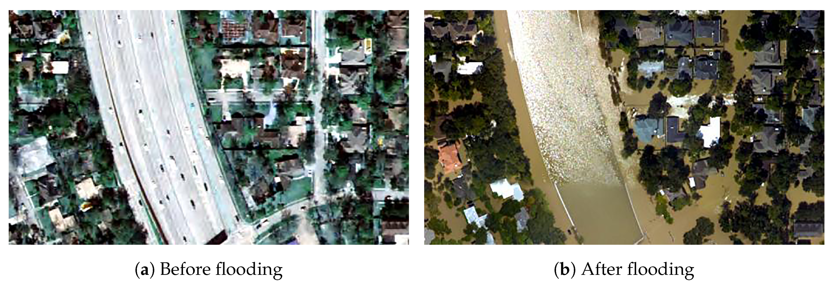
10], to classify each pixel into four classes including water, building, vegetation, and road. While the aforementioned studies could produce reasonable flood maps for urban areas, they required very accurate and time-consuming human annotation of training data for model training. Additionally, the VHR optical imagery usually has nonhomogeneous background due to various types of objects in the scene such as buildings, moving vehicles, and road networks. Moreover, the high-resolution optical imagery often has different pixel DNs for the same ground objects (see
Figure 1) due to highly inconsistent illumination conditions during a flood. As such, traditional flood mapping approaches may not generalize well on testing data.
Furthermore, pixel-based classifiers hardly can model the spatial relationship between sample pixels in the flooding area due to heterogeneous image background. Therefore, traditional machine learning approaches such as RF, support vector machine (SVM), maximum likelihood (ML), and recent image segmentation models (e.g., FCN) may not perform well with VHR optical imagery.
Another type of image data involves multispectral optical surface reflectance imagery which contains consistent and distinct spectral information associated with floodwaters [
2,
12,
13,
14,
15]. Li et al. [
12] performed the discrete particle swarm optimization (DPSO) for sub-pixel flood mapping using satellite multispectral reflectance imagery, the Landsat Thematic Mapper/Enhanced Thematic Mapper Plus (TM/ETM+) data. Malinowski et al. [
14] used a decision tree (DT) algorithm with various combinations of input variables including spectral bands of the WorldView-2 image and spectral indices to analyze spatial patterns of localized flooding on a riverine floodplain. More recently, Wang et al. [
15] added the spectral information, normalized difference water index (NDWI), into the traditional super-resolution flood inundation mapping (SRFIM) model to enhance the model response to floodwaters. Most of the flood mapping studies based on multispectral surface reflectance imagery, however, explored homogeneous rural areas instead of heterogeneous urban areas, where a larger number of people would be in danger during flooding.
The third type of image data widely used for natural disaster mapping is satellite synthetic aperture radar (SAR) imagery which can be acquired during the day or the night regardless of weather conditions due to radar’s longwave active signals with penetration power for imaging [
2,
3,
16,
17,
18]. Giustarini et al. [
17] introduced a Bayesian approach to generate probabilistic flood maps based on SAR data. Shen et al. [
16] developed a near real time (NRT) system for flood mapping using SAR data, which involves classification based on statistics, morphological processing, multi-threshold-based compensation, and machine-learning correction. Li et al. [
3] proposed an image patch classification model to map the flooded urban area with multi-temporal SAR imagery based on an active self-learning CNN framework, which addressed the issue of limited training data size. Although these studies based on SAR data made significant efforts to improve the accuracy of flood maps, the proposed models were usually complicated in terms of model architectures, and did not perform with very satisfying results in terms of overall accuracy, precision, recall, and F1 score. Moreover, for neural network based deep learning models, a large number of human annotated training samples were required.
Leveraging the advantages of different types of data, Rudner [
2] proposed to fuse multimodal satellite data (i.e., VHR optical imagery with raw pixel DNs, multispectral reflectance imagery, and SAR imagery) in a CNN model for flooded building detection in urban areas. As such, the spatial, spectral, and temporal information was integrated to improve the segmentation of flooded ground objects. However, the models discussed above required data from multimodal sensors, some of which might be missing during floods.
With regard to the mapping methods, most of literature focused on pixel-based dense classification approaches such as artificial neural network (ANN) [
19], SVM [
18], DT [
14], RF [
8], HMT [
7], particle swarm optimization (PSO) [
12], and deep CNN such as FCNs [
6], U-Net [
20], and Deeplab [
21]. While pixel-based image segmentation approaches in the aforementioned studies could generate higher resolution flood maps, they depend on high resolution flooding masks for model training, which require intensive human annotation of training samples. The annotation process might be even more expensive for urban areas as they are more heterogeneous than rural areas. As such, these models might not be able to perform in near real time when flooding occurs in urban areas.
Some of the studies also investigated patch-based classification methods for land cover mapping, which have the potential for urban flood mapping. Traditional machine learning approaches have been widely used for image scene classification. Gong et al. [
22] compared SVM, DT, and RF for Landsat image scene classification and showed that SVM performed with the highest overall accuracy. Heydari et al. [
23] also reported the superior classification performance of SVM on 26 testing blocks of Landsat imagery in comparison with ANN and the ensemble of DT. More recently, CNN based deep learning approaches have shown promising performance for image classification, such as AlexNet [
24], VGGNet [
25], GoogLeNet [
26], and ResNet [
27]. Most of these neural network models are very deep in terms of the number of layers, which are not necessary for classification of small patches as demonstrated in [
28,
29]. Sharma et al. [
28] developed a patch-based CNN model tailored for medium resolution (pixel size = 30 m) multispectral Landsat-8 imagery for land cover mapping, which outperformed pixel-based classifier in overall classification accuracy. Song et al. [
29] designed a light CNN (LCNN) model to map the land cover also using Landsat-8 imagery and achieved better results than pixel-based classifiers particularly at heterogeneous pixels, which are very common in urban areas. Additionally, traditional machine learning approaches (e.g., SVM and RF) were also tested and showed competitive results for patch-based classification compared with LCNN. It was also demonstrated that the patch-based approach has an advantage in large scale mapping in terms of computation time. Most recently, with a focus on urban flood mapping, Li et al. [
3] proposed a patch-based active self-learning CNN framework to map the flooding areas in urban Houston with multi-temporal SAR imagery. However, there still exist great potentials to simplify the model architecture and improve the F1 score and overall accuracy. Additionally, patch-based approaches to flood mapping especially over urban areas are still not well investigated. Moreover, considering the advantage of multispectral surface reflectance data, the extensive and quantitative study of patch-based urban flood mapping with multi-temporal multispectral surface reflectance imagery is still lacking. Furthermore, there has been an increasing number of available remote sensing data provided by private sectors (e.g., Planet Labs [
30] and DigitalGlobe) and government agencies (e.g., NOAA). Such a huge volume of satellite or aerial imagery presents a significant challenge to traditional machine learning approaches in data analysis. Therefore, it is imperative to develop scalable and efficient algorithms for high throughput computing given such big data that near real-time flood mapping could be acquired.
To address the aforementioned challenges, we proposed a patch similarity convolutional neural network (PSNet) with two variants (i.e., PSNet-v1 and PSNet-v2) to map the flooding extent in urban areas using satellite multispectral surface reflectance imagery before and after flooding with a spatial resolution of 3 meters. It is worth noting that we used surface reflectance instead of raw pixel DNs to alleviate the impact of inconsistent illumination and different weather conditions at the time of data collection. As a result, corresponding ground objects from the bi-temporal (pre- and post-flooding) imagery would have consistent surface reflectance. Similar to the studies in [
6,
7,
8,
29], we conducted extensive experiments with PSNet and other baseline methods including SVM, DT, RF, and AdaBoost (ADB), using two datasets: (1) the 2017 Hurricane Harvey flood in Houston, Texas, and (2) the 2018 Hurricane Florence flood in Lumberton, North Carolina. We used default parameters in scikit-learn [
31] for experiments with baseline methods as in [
7]. Experiment results showed that the PSNet with bi-temporal data achieved superior performance in F1 score and overall accuracy compared with baseline methods (i.e., SVM, DT, RF, and ADB) with either uni- or bi-temporal data.
Main contributions of this work are summarized in the following:
The proposed PSNet is a simplified two-branch CNN-based data fusion framework, performing urban flood extent mapping with pre- and post-flooding satellite multispectral surface reflectance imagery. Uni-temporal image patch classification with only post-flooding imagery was transformed into bi-temporal patch similarity estimation with both pre- and post-flooding data. Compared to uni- or bi-temporal SVM, DT, RF, and ADB, PSNet performed consistently better in F1 score and overall accuracy.
This research demonstrated that multispectral surface reflectance data play a significant role in floodwater detection. Compared with raw pixel DNs, surface reflectance is more stable under varied inconsistent illumination conditions.
The study paves the way to fuse bi-temporal remote sensing images for near real-time precision damage mapping associated with other types of natural hazards such as earthquakes, landslides, wildfires, etc.
2. Materials and Methods
2.1. Preliminaries
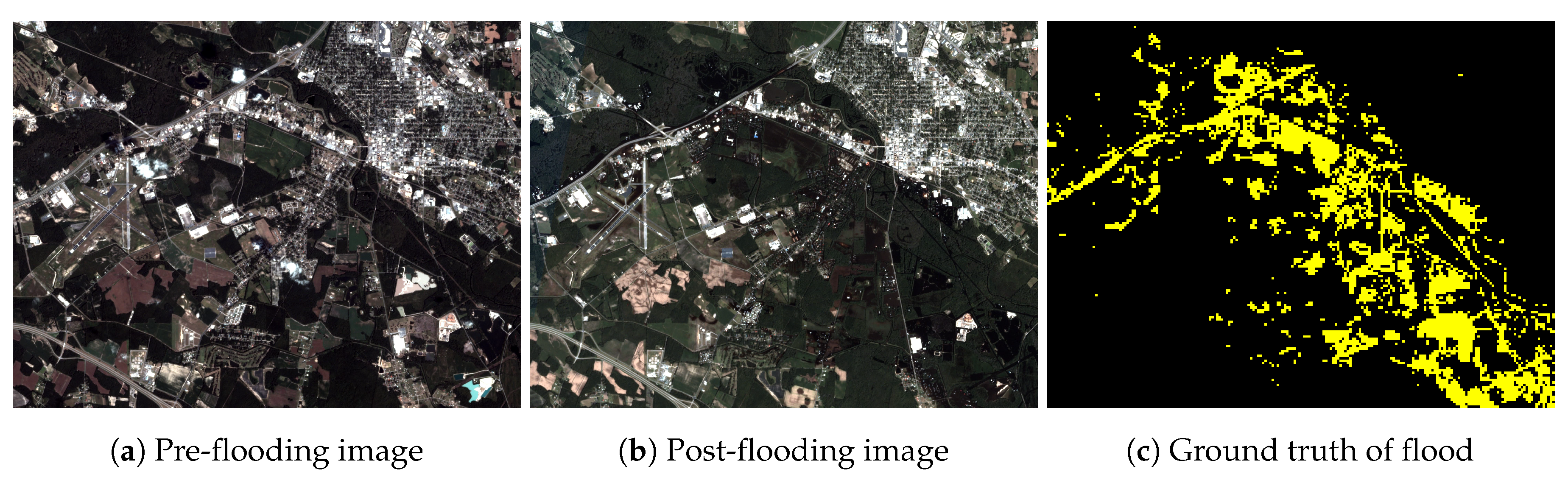
Flood extent mapping is a process to identify the land areas impacted by flooding. Various definitions of such flooding areas have been proposed [
3,
6,
7,
8]. For example, only land areas covered by visible floodwaters are considered as being flooded [
6,
8]. However, according to the National Flood Mapping Products from the Federal Emergency Management Agency (FEMA) [
32], small areas covered by invisible floodwaters due to trees or surrounded by floodwaters are also treated as being flooded [
3,
7] (see
Figure 2).
For urban flood mapping with high spatial resolution imagery, this paper uses FEMA’s definition of flood hazard zones as previous works [
3,
7] considering expensive pixel-wise flood labeling.
This study proposed to map urban flooding areas using bi-temporal pre- and post-flooding satellite multispectral surface reflectance imagery. Given the bi-temporal co-registered satellite images (before flooding) and (after flooding), this work aims at developing a binary classification model F which takes (, ) as input and returns a binary flood hazard map O as output, , where each pixel in is classified as 1 (flood, FL) or 0 (non-flood, NF).
While incorporating bi-temporal imagery for flood mapping over heterogeneous urban areas, it is worth noting that and may not align well. Corresponding pixels, and , at the same geographical location, may not exactly refer to the same ground object even though and are co-registered. This may be due to three major reasons: (1) trees grow and therefore display differently in multi-temporal imagery acquired over different seasons; (2) moving objects (e.g., cars) are quite common over urban areas; and (3) ortho-rectification of and may not be perfect due to complex terrains and ground infrastructures (e.g., tall buildings). As a result, pixel-based analysis of multi-temporal imagery may not perform well for urban flood mapping. To overcome the limitation of high heterogeneity over the urban area, this work conducted patch-based flood mapping.
2.2. Datasets
We studied two flooding events caused by severe hurricanes over the urban areas. One is west Houston, Texas, which was flooded due to the Hurricane Harvey in August 2017. The other is the city of Lumberton, North Carolina, which was flooded as a result of the Hurricane Florence in September 2018.
The data used in this study were satellite imagery from the Planet Lab [
30] with a spatial resolution of 3 m, and four spectral bands including blue (B), green (G), red (R), and near infrared (NIR) (see
Table 1). All imagery were orthorectified and radiometrically calibrated into surface spectral reflectance such that the data are more independent from weather conditions. In addition, the bi-temporal pre- and post-flooding imagery were co-registered for similarity analysis.
The Harvey pre- and post-flooding satellite multispectral images over west Houston, Texas, were collected on 31 July 2017 and 31 August 2017, respectively (
Table 1). The bi-temporal images were split into non-overlapping patches of spatial size
. Since the spatial resolution of the satellite images (i.e., pixel size) is 3 m, all image patches cover a ground area of 42 m
m (
). The patch size was set to a similar value used in a most recent study on urban flood mapping [
3], in which patches of size 40 m × 40 m were cropped from the original SAR imagery. Therefore, patch-based classification in this study for mapping flooded urban areas can be compared qualitatively with the existing work [
3]. Regarding the annotation for the classes of post-flooding satellite multispectral patches, two classes are defined including flooded (FL) patches with floodwaters and non-flooded (NF) patches without floodwaters, and image patches without visible floodwaters were annotated as NF [
3]. During the annotation, aerial VHR optical images with a spatial resolution of 0.3 m collected by NOAA on 31 August 2017 were used as reference. Specifically, we used the aerial VHR optical image with the same ground coverage as the Harvey pre- and post-flooding satellite multispectral images. Non-overlapping patches of size
were cropped from the VHR image such that each VHR patch corresponds to a pair of pre- and post-flooding satellite multispectral patches. As each VHR patch covers the same ground area (i.e., 140 × 0.3 = 42 m) as the satellite multispectral patch, the satellite multispectral patches were labeled by visual inspection of the corresponding VHR patches. Therefore, we obtained 28,908 annotated patches, of which 8517 are in class FL and 20,391 are in class NF.
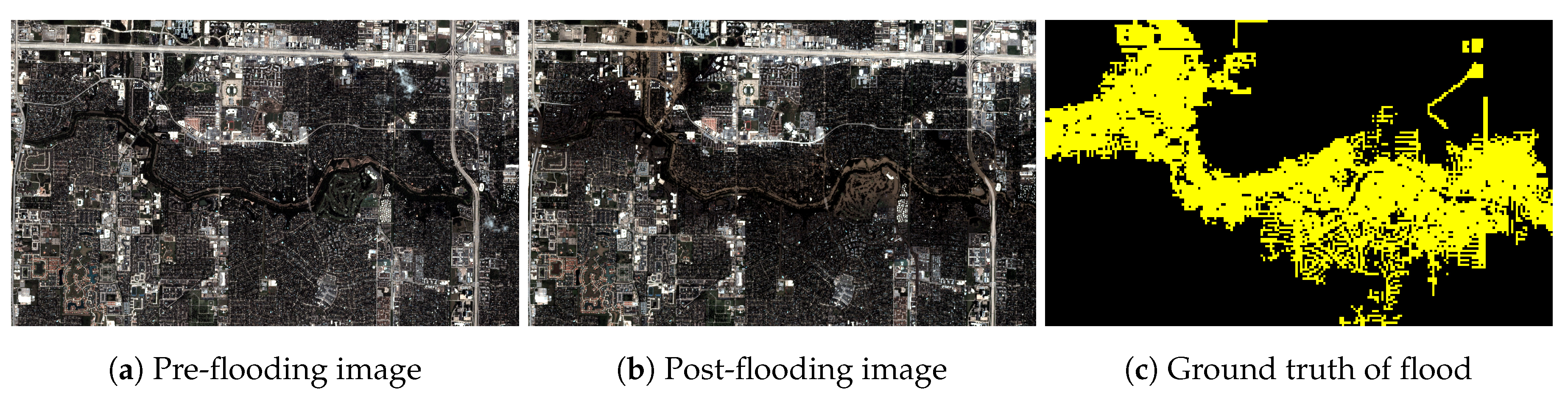
Figure 3 shows the Harvey pre- and post-flooding satellite multispectral surface reflectance images with ground truth over the whole study area. For model training and evaluation, we randomly sampled 5000 pairs of patches from the bi-temporal pre- and post-flooding dataset for training and validation, whereas the rest of samples (23,908) were used for testing.
The Florence pre- and post-flooding satellite images with corresponding ground truth of flood map (
Figure 4) over the Lumberton city were acquired on 30 August 2018 and 18 September 2018, respectively (
Table 1). Similar to the data pre-processing for Hurricane Harvey, 33,600 annotated patches were obtained, of which 5003 are in class FL and 28,597 are in class NF. We randomly sampled 5000 samples for model training and validation, and kept the remaining 28,600 for testing.
For both Harvey and Florence data with 5000 samples for training and validation, 4000 samples were used for training while the rest 1000 samples were fixed for validation and model selection.
2.3. Methods
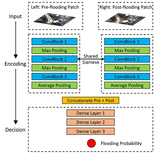
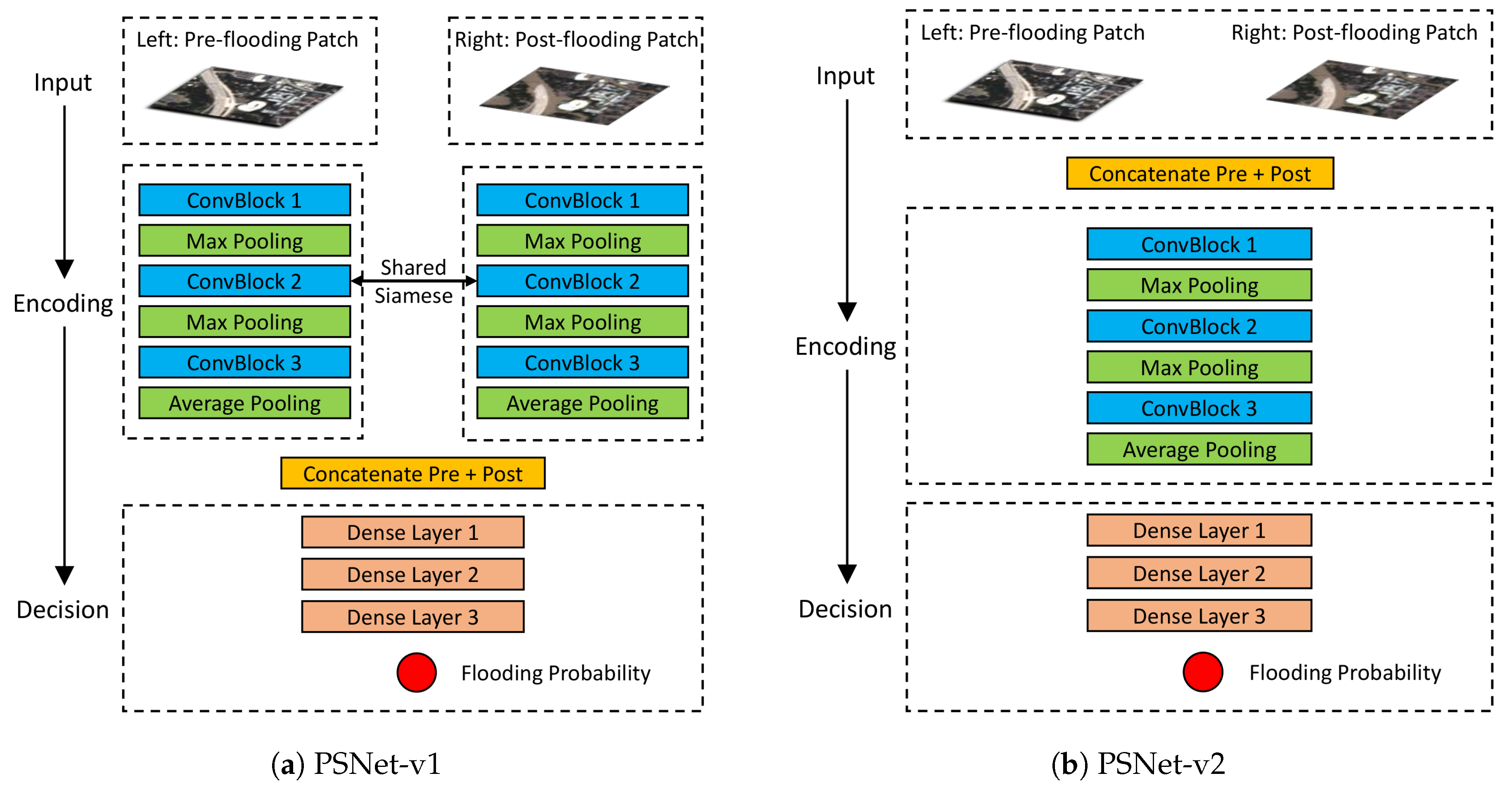
Patch Similarity Evaluation
The bi-temporal satellite images, , were divided into non-overlapping image patches, and , of the same size. Each pair of patches covers the same geographic area. Therefore, instead of classifying each pixel pair, and , we predict the class of each patch pair, and , to be either FL or NF. In this study, we evaluate the flooding probability of each patch pair, and , based on their similarity. Note that we assume that the major dissimilarity between and is resulted from flooding since the pre- and post-flooding images were collected intermediately before and shortly after the flooding event, respectively. Accordingly, the patch similarity is negatively correlated with the probability that the patch pair under test is flooded. The less similar are and , the more likely they are of being flooded.
This work proposed the PSNet to learn the nonlinear mapping from the pre- and post-flooding patch pairs,
and
, to the output class, FL or NF. Two variants (PSNet-v1 and PSNet-v2) of the network architecture are shown in
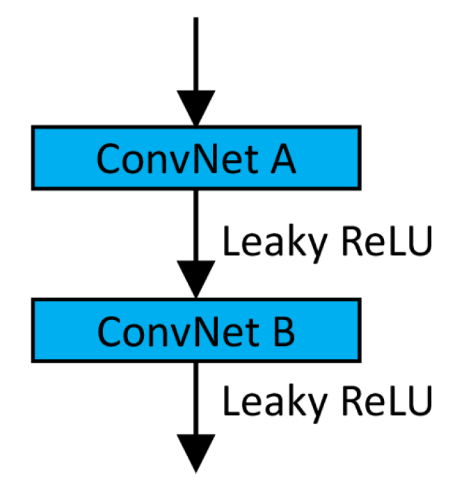
Figure 5a,b, respectively, in which the convolutional block (ConvBlock) is shown in
Figure 6. The PSNet in this work basically consists of two modules,
Encoding and
Decision.
The
Encoding module learns the feature representations from the input pre- and post-flooding patches, respectively. More specifically, in PSNet-v1, the
Encoding module has a Siamese sub-network architectures on the left and right paths to learn the feature representations from the pre- and post-flooding patches. To perform similarity analysis in the
Decision module, the left and right sub-networks share the weights [
33], which in turn alleviates the computing load. The sub-network in the
Encoding module contains a stack of ConvBlocks (
Figure 6). Feature representations of pre- and post-flooding patches from the left and right paths would then join after the
Encoding module through concatenation along the channel dimension. Different from PSNet-v1, the other variant PSNet-v2 first concatenates the pre- and post-flooding patches and then feeds the patch stack into the
Encoding module for joint feature learning.
The
Decision module evaluates the similarity between the feature representations learned from the pre- and post-flooding patches through the
Encoding module. It performs binary classification (i.e., FL or NF) by taking as input the joint feature representations, and following a set of dense layers. Detailed settings and hyperparameters of the architecture of PSNet-v1 are listed in
Table 2. PSNet-v2 was developed with similar set of hyperparameters used for PSNet-v1.
2.4. Evaluation Metrics
For all experiments, we evaluated the overall accuracy (OA), precision, recall, and F1 score [
34,
35,
36], which are defined in Equation (
1).
where
denote the number of true positives, false positives, true negatives, and false negatives, respectively. For comparative analysis, we performed patch classification with baseline algorithms: support vector machine (SVM), decision trees (DT), random forest (RF), and AdaBoost (AdB). We tested all baselines with uni-temporal data (i.e., post-flooding patches ) and bi-temporal data (i.e., pre- and post-flooding patches).
2.5. Model Training and Testing
For training supervised PSNet, we take as input the pre- and post-flooding patch pairs and as target the corresponding true labels (FL or NF). The Adam optimizer [
37] is applied with batched patch pairs to minimize the weighted binary cross entropy loss,
, defined as Equation (
2).
where
x is the output of the network (i.e., the probability of being flooded),
y is the target label,
N is the number of patch pairs in a batch, and
is the weighted cross entropy loss for the
ith patch pair with associated weight
. We assigned different weights for the class FL and NF due to high class imbalance of the training data. The sample weight is defined as the complementary of its occurrence frequency in the training set. More specifically, with regard to the training set including
FL and
NF samples, we set the weights of FL and NF samples as
and
, respectively.
All models were trained with batched samples for 200 epochs. We initialized the learning rate to be and divide it by 10 when observing no further decrease of validation loss. Weight decay of and momentum parameters for the Adam optimizer were used during training. Considering limited size of the training data, data augmentation was used to enhance the model generalization capability, including random horizontal and vertical flip, rotation of degrees in , and normalization of pixel reflectance into the range of .
Before the training process, good weight initialization is important for networks with multiple paths to avoid partial node activation [
20]. In this study, the weights were initialized by random sampling from the Gaussian distribution,
∼
, where
V is the number of associated parameters for each node. More specifically, for a
convolutional kernel with
C channels in the previous layer,
.
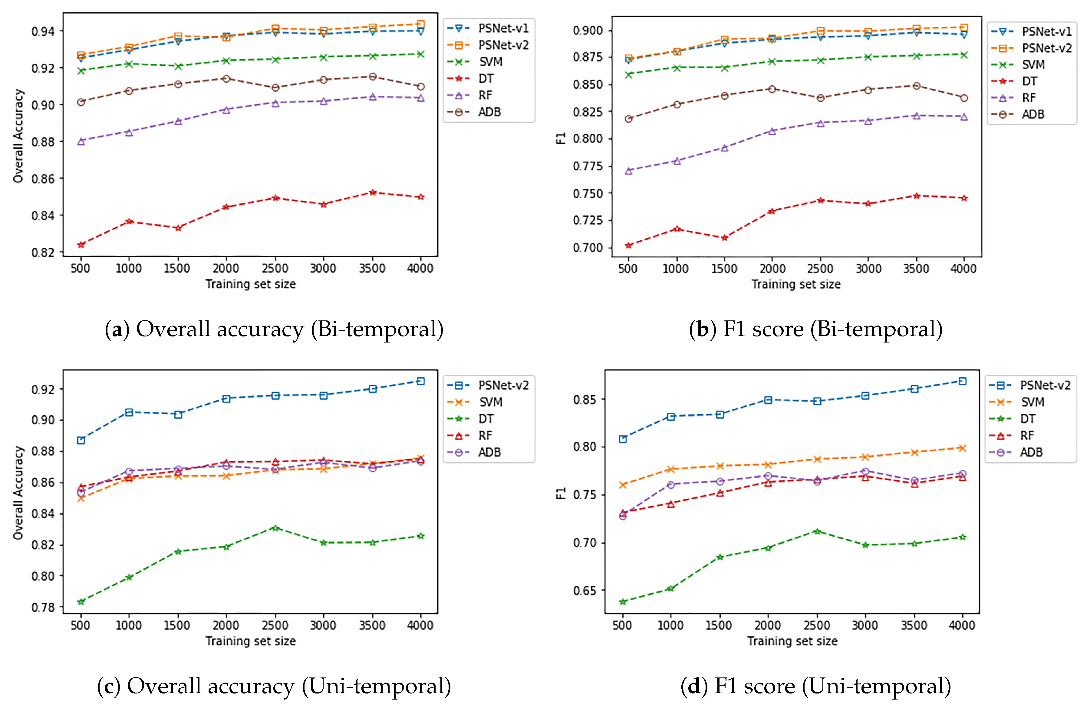
To investigate how the training set size may influence the classification performance, we trained all models with different sizes of training set. Specifically, we randomly sampled various numbers of training samples from the original training subset of size 4000 and trained multiple PSNet models. Fixed validation and testing subsets were used for model selection and performance evaluation. In this work, we selected trained models with highest validation F1 scores for testing.
All experiments of PSNet were conducted with PyTorch [
38] on a Dell workstation with 16 GiB Intel(R) Xeon(R) W-2125 CPU @ 4.00 GHz × 8, 8 GiB Quadro P4000 GPU, and 64-bit Ubuntu 18.04.2 LTS.
4. Discussions
Unlike pixel-based classification for flood mapping [
6,
7,
8,
12,
39,
40], this study investigated image patch based flood mapping similar to the study in [
3]. Major motivations include: (1) reducing the impact of heterogeneous image background over urban area, which is challenging for pixel-based classification; and (2) accelerating human annotation of training samples since pixel-wise labeling would be much more time-consuming and labor-intensive.
Similar to the studies in [
3,
6,
7,
8,
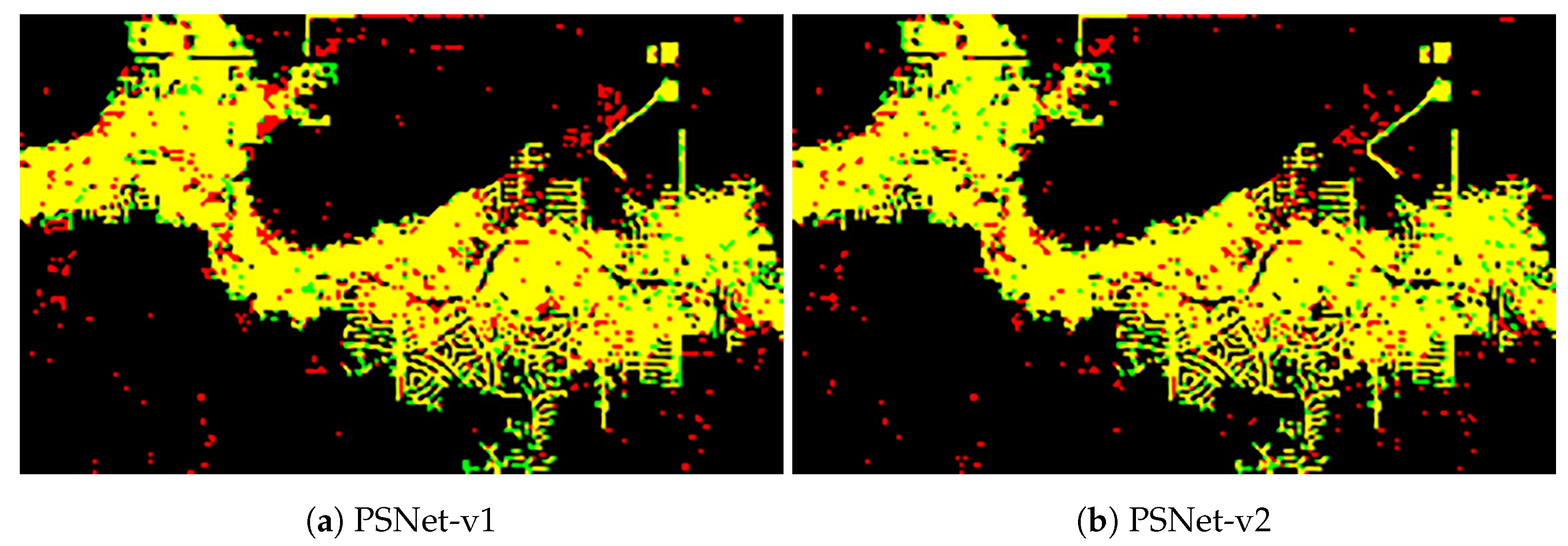
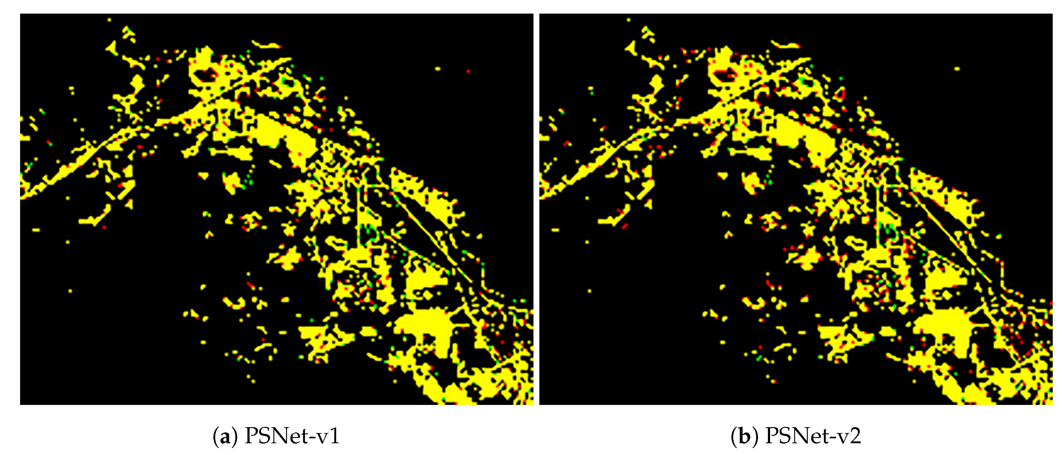
29] for comparative analysis, we performed patch-based classification with traditional machine learning models as baselines, including SVM, DT, RF, and ADB. The experiment results of the two urban flood events (i.e., the 2017 Hurricane Harvey flood and the 2018 Hurricane Florence flood) demonstrate the superior performance of the proposed PSNet over all baseline algorithms (
Figure 7 and
Figure 9 and
Table 3 and
Table 4). With regard to patch-based classification models, the PSNet developed in this study leveraged an efficient two-branch data fusion framework specifically for urban flood mapping. It is worth noting that the
Encoding module can be developed with different variants of the patch-based CNN architecture used in this study. As a result, the specific architecture of the
Encoding module along with its hyperparameters used in this study can be considered as a representative of patch-based CNN encoding for the input patches. This work did not experiment with image segmentation models (e.g., FCNs, U-Net, and Deeplab) since image segmentation works for pixel-based, instead of patch-based, dense classification. In addition, we did not compare with deep image classification models, such as AlexNet, VGGNet, GoogLeNet, and ResNet, since classification of small patches does not require such deep architectures [
28,
29]. With regard to other CNN-based patch classification models discussed in [
28,
29], direct comparison is not valid due to different input dimensions and image resolutions, which require major modification of the
Encoding module architectures and tuning of hyperparameters.
More specifically, regarding patch-based urban flood mapping, this study followed the experimental settings of a recent research for urban flood mapping with SAR data [
3], in which the study area (i.e., west Houston) is smaller than the one investigated in this study. For reference, we used patches of size 14 × 14 to cover the ground area of 42 m × 42 m, which is close to the area (i.e., 40 m × 40 m) covered by patches used in [
3]. We did not experiment with the exact same size of patches due to the constraint of different spatial resolutions of images used in the two studies. It should be noted that we labeled all patches with floodwaters as being flooded, whereas, in [
3], only patches that were severely flooded were labeled as being flooded. In other words, there are fewer patches in [
3] labeled as being flooded than that of this study. For patches that were partially covered by floodwaters but not heavily flooded, the classification model would have very poor response. Therefore, the results in this study cannot be directly and quantitatively compared with those in [
3]. For qualitative comparison regarding the Harvey flooding event, as reported in [
3], the developed active self-learning CNN model detected flooded patches with precision of 0.684, recall of 0.824, F1 score of 0.746, and overall accuracy of 0.928 when using model trained with 600 pre- and post-flooding SAR patches. However, this study achieved the performance with precision of 0.848, recall of 0.906, F1 score of 0.873, and overall accuracy of 0.925 with model (PSNet-v1) trained with 500 bi-temporal multispectral patches (
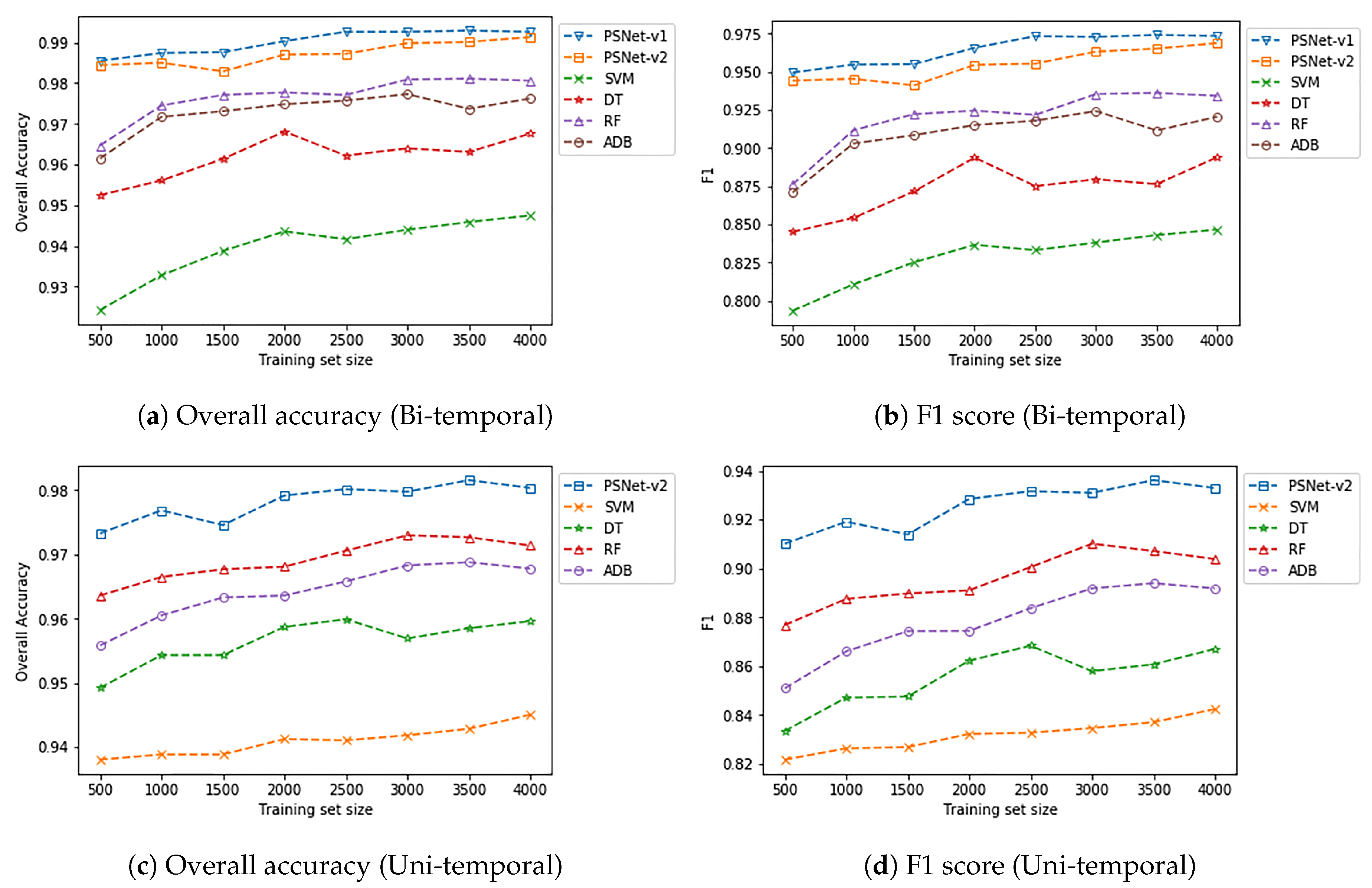
Table 5). In addition, the PSNet was designed with simple architectures for easy implementation. More importantly, it shows that only a small number (e.g., 500) of training samples are needed for training a competitive model (PSNet) that generalizes well on the testing data, and thus contributes to quick mapping of the flooding area.
With experiments on both uni- and bi-temporal data, the results show that bi-temporal pre- and post-flooding data contribute significantly to boosting the performance of PSNet for patch similarity analysis and thus for flooded patch identification. Patch similarity learning has proved to be effective in patch-based matching of stereo images [
33,
41,
42,
43]. Due to the heterogeneity of the satellite image background over urban areas, patches of class FL usually have various patterns which are difficult to be learned by the classification algorithms with a very limited number of training samples. As shown in
Figure 7 and
Figure 9, patch similarity evaluation based PSNet with bi-temporal data consistently outperformed those floodwater pattern recognition based models with uni-temporal data. It is worth noting that, with only 500 training samples, the proposed PSNet was able to perform with, approximately, a F1 score of 0.87 and an overall accuracy of 0.93 on Harvey testing data. Similar high performance can also be observed in the experiment for the Florence data.
We investigated the important role of spectral reflectance in urban flood mapping. As spectral reflectance has been recognized as the signature of ground objects [
44], it would be more invariant with respect to illumination conditions. Therefore, with only a small number of human annotated samples (e.g., 1500), we could identify the flooded image patches with around 0.8914 F1 score and 0.9371 overall accuracy for Harvey testing data (
Table 3), and 0.9551 F1 score and 0.9876 overall accuracy for Florence testing data (
Table 4), which are consistently better than the results produced by the baseline algorithms. Compared with studies using SAR imagery [
3] and optical imagery with raw pixel DNs [
8], spectral reflectance data in this study play an important role in helping PSNet achieve superior performance in urban flood mapping with merely a small number of training samples (e.g., 500), as demonstrated by the learning curves in
Figure 7 and
Figure 9.
It is worth noting that PSNet achieved higher F1 score and overall accuracy on the Florence data (
Table 4) than that on the Harvey data (
Table 3). It is mainly because the Harvey data covering the west Houston area are more heterogeneous than the Florence data covering the Lumberton city. More specifically, the west Houston area includes dense residential, industrial, and commercial regions, where various ground objects result in more heterogeneous image background. As a result, it would be relatively easier for the PSNet trained with the Florence training data to achieve better performance on the Florence testing data.
With regard to the processing time on model training and testing for creating the flood maps, it took about 6 min to train the PSNet with 500 samples and 1 min to create the flood map of the study area (e.g., west urban Houston) on the Dell workstation used in this work. The running time associated with traditional approaches (e.g., SVM, DT, RF, and ADB) is even less than the PSNet. As such, the time consumption on PSNet training and testing can be ignored for near real-time urban flood mapping. It should be noted that the major time-consuming process is human annotation of training samples. In this study, three research assistants could label 500 training samples in less than 20 min, which can also be ignored for near real-time urban flood mapping.
To sum up, the major strength of the proposed PSNet with bi-temporal data is to map the urban flooding area with high overall accuracy and F1 score, as demonstrated by the quantitative results in
Figure 7 and
Figure 9. More detailed evaluation results over all metrics corresponding to 1500 training samples can be found in
Table 3 and
Table 4. One major limitation of this study in practice is that part of the satellite imagery covering the flooding area may contain clouds, which is the major challenge for multispectral image analysis. In this case, further work could be dedicated to fusing both multispectral imagery and SAR imagery for joint urban flood mapping by virtue of the penetration power of the SAR signals [
2].


