Assessing the Use of Sentinel-2 Time Series Data for Monitoring Cork Oak Decline in Portugal


Instituto Dom Luiz (IDL), Faculdade de Ciências, Universidade de Lisboa, 1749-016 Lisboa, Portugal
*
Author to whom correspondence should be addressed.
Remote Sens. 2019, 11(21), 2515; https://0-doi-org.brum.beds.ac.uk/10.3390/rs11212515
Submission received: 27 September 2019
/
Revised: 23 October 2019
/
Accepted: 24 October 2019
/
Published: 28 October 2019
(This article belongs to the Section Remote Sensing in Agriculture and Vegetation)
Abstract
:In Portugal, cork oak (Quercus suber L.) stands cover 737 Mha, being the most predominant species of the montado agroforestry system, contributing to the economic, social and environmental development of the country. Cork oak decline is a known problem since the late years of the 19th century that has recently worsened. The causes of oak decline seem to be a result of slow and cumulative processes, although the role of each environmental factor is not yet established. The availability of Sentinel-2 high spatial and temporal resolution dense time series enables monitoring of gradual processes. These processes can be monitored using spectral vegetation indices (VI) as their temporal dynamics are expected to be related with green biomass and photosynthetic efficiency. The Normalized Difference Vegetation Index (NDVI) is sensitive to structural canopy changes, however it tends to saturate at moderate-to-dense canopies. Modified VI have been proposed to incorporate the reflectance in the red-edge spectral region, which is highly sensitive to chlorophyll content while largely unaffected by structural properties. In this research, in situ data on the location and vitality status of cork oak trees are used to assess the correlation between chlorophyll indices (CI) and NDVI time series trends and cork oak vitality at the tree level. Preliminary results seem to be promising since differences between healthy and unhealthy (diseased/dead) trees were observed.
1. Introduction
Cork oak (Quercus suber L.) woodlands are one of the most representative forest ecosystems characterizing the Western Mediterranean region. This species occurs spontaneously in Portugal mainland, usually forming low density stands with open heterogeneous canopies in silvo-pastoral ecosystems, named montado. According to the Portuguese National Forest Inventory, eucalyptus (mainly Eucalyptus globulus) is the dominant species (812 Mha; 26%), but cork oak (737 Mha; 23%) and maritime pine (714 Mha; 23%) stands are equally representative [1].
In Portugal, the importance of cork oak has been recognized by law since the 13th century. Cork oak was even unanimously established as Portugal’s National Tree in 2011, mostly due to its economic, social and environmental relevance. Besides the importance of the cork industry, it also promotes local population employment and contributes for the preservation of a wide range of flora and fauna habitats. Legislation protecting cork oak stands forbids the felling of trees, meaning that only dead or diseased trees can be felled but only with a permission from the National Nature Conservation and Forest Authority (ICNF).
A significant cork oak decline has been observed in Portugal over the last decades. Land management practices, rather than environmental factors, seem to be the main trigger of changes in the phytosanitary conditions of cork oak trees [2]. Besides, land use disturbances, mostly associated to intensity/type of grazing and shrub encroachment, tree water stress is an additional cause of decline [3]. As reported by Besson et al. [4], changes in climate conditions (water scarcity or excessive soil moisture) are stressing cork oak trees. As stated in the last International Panel on Climate Change (IPCC) assessment report [5], mean annual temperature has been rising while precipitation has been decreasing, in the Mediterranean region, for the past decades foreseeing a higher frequency of extreme drought and rainfall events. The impact on water resources is causing the lowering of groundwater levels which consequently has a negative effect on cork oak growth since it relies on deep rooting to access the groundwater table [6]. Additionally, Tiberi et al. [7] have reported that insect pests and plant pathogens may act synergistically with both mismanagement and adverse climatic factors accelerating the onset of decline.
Although being an evergreen tree, canopy renewal occurs mainly during early spring. This means that cork oak trees perform photosynthesis for a longer period during the year, when compared to other broad-leaved trees that lose their leaves during winter. This makes the use of vegetation indices (VI) suitable to monitor cork oak phenology and identify leaf phenological events. Normalized Difference Vegetation Index (NDVI) [8] showed a good relationship with cork production at the forest stand level [9], revealing that one-tenth of the area of cork and holm oak stands in mainland Portugal have significant declining trends over a 34-year period. This trend, identified using a summer NDVI (July and August) time series obtained from Landsat and MODIS imagery, did not result from short-term events, such as droughts or debarking, but reflects a long-term evolution of the forest stands health. A 15-year Enhanced Vegetation Index (EVI) time series and micrometeorological data was used by Santos et al. [10] to evaluate if the relationship between cork oak woodlands productivity, in Southern Portugal, and climate is affected by the combined response of trees, shrubs and grassland. EVI trends, obtained also from Landsat data, showed differences in oaks and shrubs productivity that were positively related with relative humidity and negatively with temperature, suggesting that cork oak seems to be more resilient or having lagged responses to climate change than shrubs and grassland.
The European Copernicus program with its Sentinel-2 satellites provides high (10 m) optical spatial resolution data at higher temporal frequencies (5 day revisit with two operational satellites) than previously available with the Landsat data. Besides, it provides red-edge spectral data that combines both sensitivity to chlorophyll content and leaf area variation. Cork oak red-edge spectral response from Sentinel-2 was compared with Landsat-8 data and in situ observations for mapping and monitoring cork oak woodlands in the Calabria region (Southern Italy) [11]. As expected, and despite the bandwidth proximity of the two sensors, Normalized Difference Red-Edge (NDRE) vegetation index [12] provided more details on cork oak phenology than NDVI obtained from Landsat-8 data, significantly improving its discrimination from other broad-leaved woodlands. In line with these results, Zarco-Tejada et al. [13] demonstrated that gradual decline processes affected the entire red-edge spectral region. In fact, red-edge chlorophyll index (CI) vs. NDVI temporal rates of change for healthy trees differ from the ones observed for trees under decline.
The main goal of this research was to evaluate the potential of using Sentinel-2 imagery for the annual monitoring of cork oak vitality. We propose a strategy to monitor cork oak vitality through spaceborne remote sensing and to provide information to forestry farmers about diseased and/or dead trees on an annual basis. Taking advantage of the Sentinel-2 mission continuity, it becomes possible to monitor long-term phenomena based on its multi-spectral high-spatial and temporal resolution optical observations. The use of dense VI time series is assessed in order to ensure a periodic monitoring of the cork oak vitality at the tree level and, consequently, the identification of diseased and/or dead trees. An annual inventory of dead trees would be extremely useful to simplify the tree felling procedure, which requires first the identification of all individual trees on the field (marked as diseased using a white painted band), followed by a permission from ICNF and finally an inspection by the field technicians. Two cork oak stands of around 15 ha and 45 ha located northeast Lisbon (Ribatejo province), are used to assess the relationship between VI trends and cork oak forests vitality. This research was developed in the scope of the GEO SUBER project, funded by the Financing Institute for Agriculture and Fisheries (IFAP) through the European Agricultural Fund for Rural Development (EAFRD).
2. Materials and Methods
2.1. Test Sites
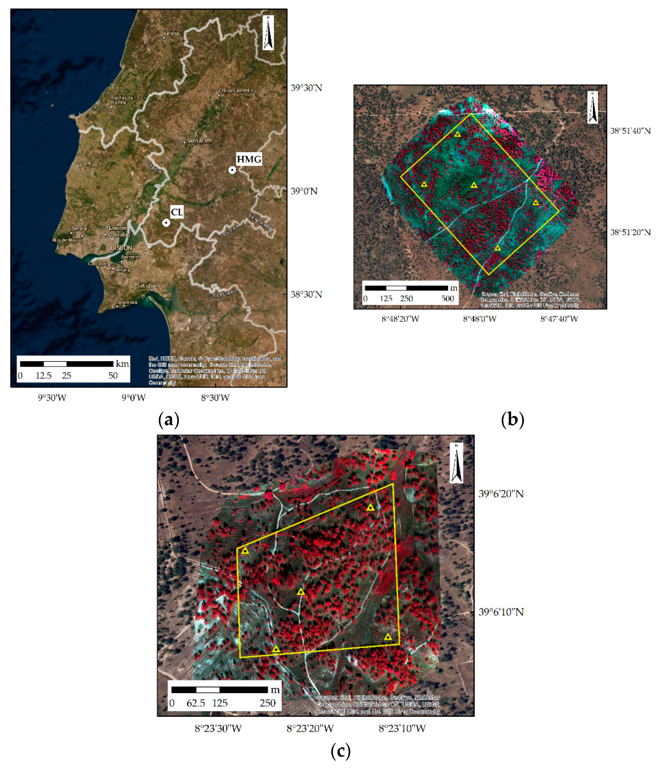
The study was undertaken in two agro-silvo-pastoral systems located in central Portugal, namely in Companhia das Lezírias (site CL) and Herdade da Machoqueira do Grou (site HMG) (Figure 1). Site CL has a total area of around 46.1 ha while site HMG has approximately 14.6 ha. Both sites are located northeast Lisbon in the Ribatejo province. Companhia das Lezírias lies between the Tagus and the Sorraia Rivers and is divided by a national road into north and south Lezíria, while Herdade da Machoqueira do Grou is located at the left bank tributary of the Tagus River, approximately 100 km of Lisbon. This region is characterised by a mild Mediterranean climate with Atlantic influences. The bioclimate is considered semiarid to subhumid, with a mean average annual rainfall of 662.5 mm and a mean annual temperature of 16.3 °C.
Companhia das Lezírias is the biggest agro-silvo-pastoral system in Portugal with a total area of around 18,000 ha. Within its limits, four different tree species stands (maritime pine, stone pine, cork oak and eucalyptus) occupy an area of 8680 ha, being cork oak (Quercus suber L.) the most representative species corresponding to approximately to 78% of the total forest area. This is the biggest unbroken stretch of cork oak in the country, with an average annual productivity of 1125 ton and an average productivity of 2.17 ton per hectare. The area is low-lying (ranging from 1 to 53 m at the highest locations) and practically flat (riverside meadows and plains). The soil is composed entirely of a mixture of brown, clayey alluvial and colluvial lutum, created from fertile deposits and left by floods and tides as sediment on sandy layers.
Herdade da Machoqueira do Grou is a private agro-silvo-pastoral system with 2423 ha. Again, cork oak is the dominant species occupying an area of 1017 ha and additionally more 464 ha of mixed-tree stand with stone pine. The entire watershed is on deep Miocene sands and the main soil types include fluvisols, leptosols, and podzols. The landscape is mostly plain, with altitudes ranging from 79 to 173 m, with slopes between 0% and 5%, and exceptionally up to 35%. Cork oak average density is 90 trees/ha and the average production of dry weight cork is 1.3 tons/ha [14].
2.2. UAV Survey Campaigns
UAV visible and near infrared (NIR) imagery was collected using an eBee Classic drone equipped with a Parrot Sequoia+ multispectral camera (senseFly-Parrot Group, Cheseaux-sur-Lausanne, Switzerland). The sensor has four 1.2 MPIX global shutter single-band cameras with a focal distance of 3.98 mm and a 1280 × 960 pixel detector that capture images at four separate bands: green (centre wavelength, 550 nm), red (660 nm), red edge (735 nm) and near infrared (790 nm) with an angular field of view (FOV) of 61.9° × 48.5°. It also includes a sunshine sensor that records the intensity of light emanating from the sun in the same four bands of light. The Parrot Sequoia multispectral sensor incorporates a GPS, an inertial measurement unit (IMU) and a magnetometer, which greatly increase the accuracy of the collected data.
Aerial survey campaigns were conducted in June/July and October 2018 at both sites (Table 1). All flights were performed within a 2-h window around the solar zenith to maintain relatively constant lightning conditions. The eMotion software was used to plan the flights, allowing the definition of an automatic flight route with waypoints, depending on the camera’s FOV, the forward and side overlap between images and the required ground sampling distance (GSD). Data was acquired with 75% side overlap and 70% forward overlap at a flight altitude of around 140 m above ground level (AGL), providing images with an average GSD of 0.12 m.
2.3. Sentinel-2 Satellite Images
Sentinel-2 (S2) carries an innovative multispectral imager (MSI) that acquires high-resolution imagery at 13 spectral bands in the visible, near infrared, and short-wave infrared regions of the spectrum with 10 to 60 m spatial resolution. A single 100 km × 100 km orthoimage (tile 29SND) in UTM/WGS84 projection covers both test sites. For this study, 30 cloud-free Level-2A S2 images acquired from 25 May 2017 to 6 December 2018 were used (Table 1). Level-2A products provide Bottom-Of-Atmosphere (BOA) reflectance generated with Sen2Cor processor whose main purpose is to correct single-date Sentinel-2 Level-1C products from the effects of the atmosphere. Since surface reflectance values are coded in JPEG2000 with the same quantification value of 10,000 as for Level-1C products, a factor of 1/10,000 was applied to Level-2A digital numbers (DN) to retrieve physical surface reflectance values.
2.4. Field Campaigns
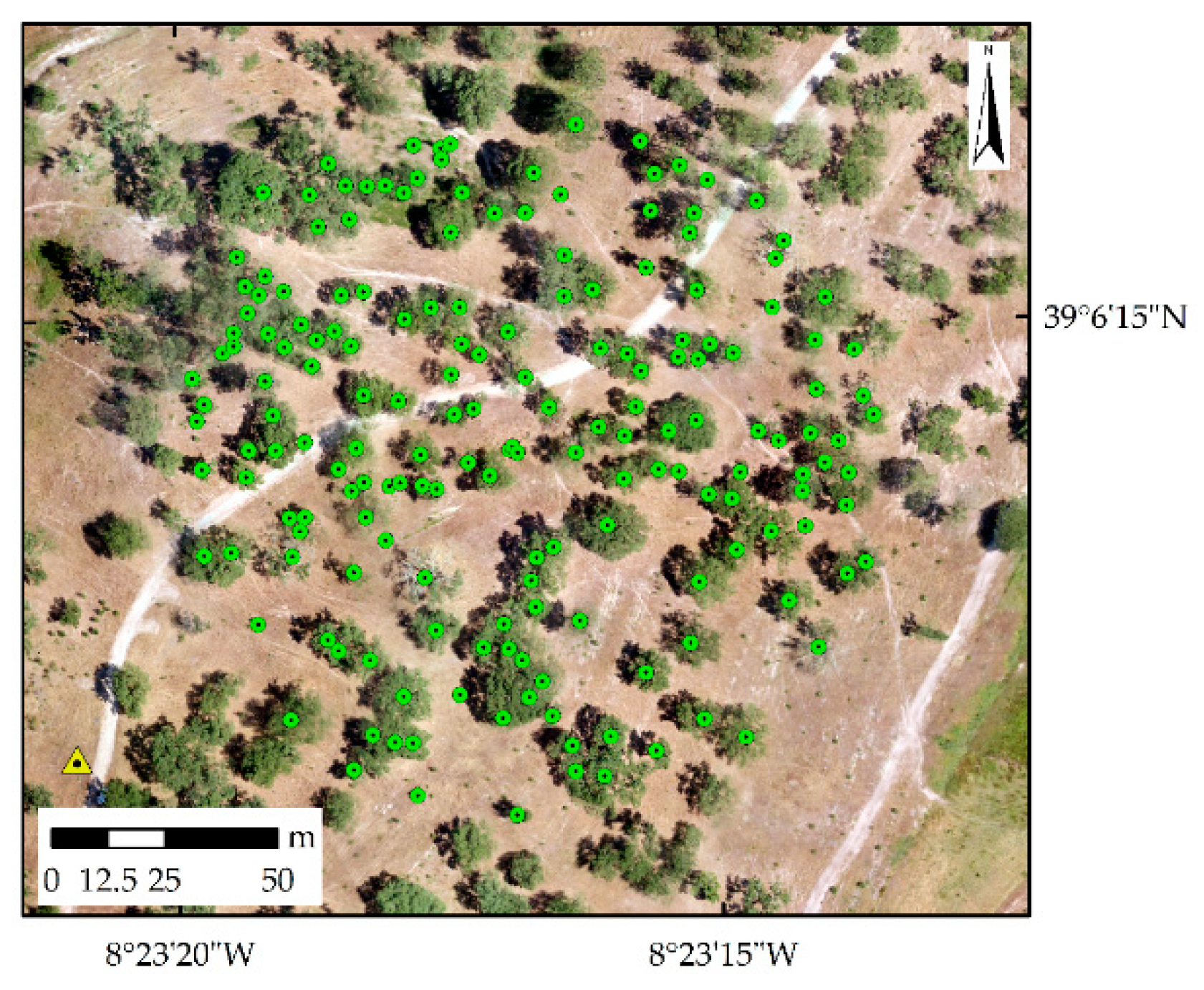
Two circular areas of 150 m diameter were defined as in situ data collection sites, one for each site (Figure 2). All cork oak trees within both circles were coordinated by RTK-GPS, corresponding to 164 trees for site CL and 182 trees for site HMG. Also, the defoliation condition of each tree was evaluated as belonging to one of 6 different classes: 0—no damage; 10—light damage; 20—moderate damage; 30—severe damage; 40—very severe damage; and 50—dead tree (Table 2). Phytosanitary and defoliation condition data were collected in several field campaigns held during October 2018. The location of each tree was edited manually by visual interpretation after field work, using the corresponding orthomosaic, in order to place all trees in their exact location. These data were used not only to identify the phenological behaviour (trend) of each tree during the time period under study but also to validate the results of the algorithm developed in this research for the automatic detection of tree crowns.
2.5. UAV Mosaic Orthorectification
UAV images were processed using the Pix4Dmapper Pro software to produce a digital surface model (DSM) and an orthomosaic for each flight. The orthomosaic was generated using the DSM that comes from the 3D densified point cloud. The DSM was generated using the Inverse Distance Weighting (IDW) algorithm in Pix4Dmapper Pro. For filtering and smoothing the points of the point cloud, a sharp noise filter and a sharp surface smoothing were used to preserve the orientation of the surface and to keep sharp features.
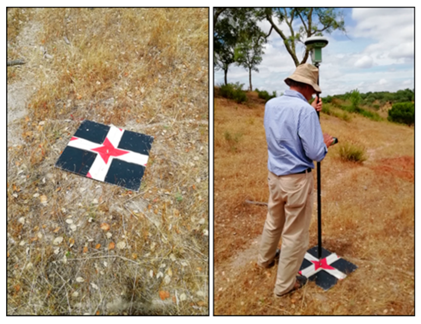
To ensure an accurate rectification of the UAV images, five ground control points (GCPs), four at the corners and one in the middle of each test site, were designed specifically for that purpose with 50 × 50 cm in size (Figure 3). RTK GPS coordinates were recorded with a positional uncertainty of 0.02 m. Root mean square errors (RMSE) were calculated to evaluate the accuracy of the bundle block adjustment. RMSE (95% confidence interval) was within 0.05 m for HMG and 0.01 m for CL, and the adopted coordinated system was ETRS89/Portugal TM06 (EPSG: 3763).
2.6. Individual Tree Crowns Identification
An algorithm for the tree crown automatic identification based on very high-resolution UAV imagery was developed using MATLAB®. Normalized Difference Vegetation Index (NDVI) and Soil-Adjusted Vegetation Index (SAVI) grayscale images were used to develop the algorithm. NDVI [8] is used basically as an indicator of canopy structure and photosynthetic activity, however it has some limitations in low to medium levels of vegetation density covers. When vegetation is sparse, with bare soil in between, the soil may affect significantly the spectral response, which is the case of cork oak woodlands. This is the reason why SAVI [15], that improves the sensitivity of NDVI to soil backgrounds, was also considered.
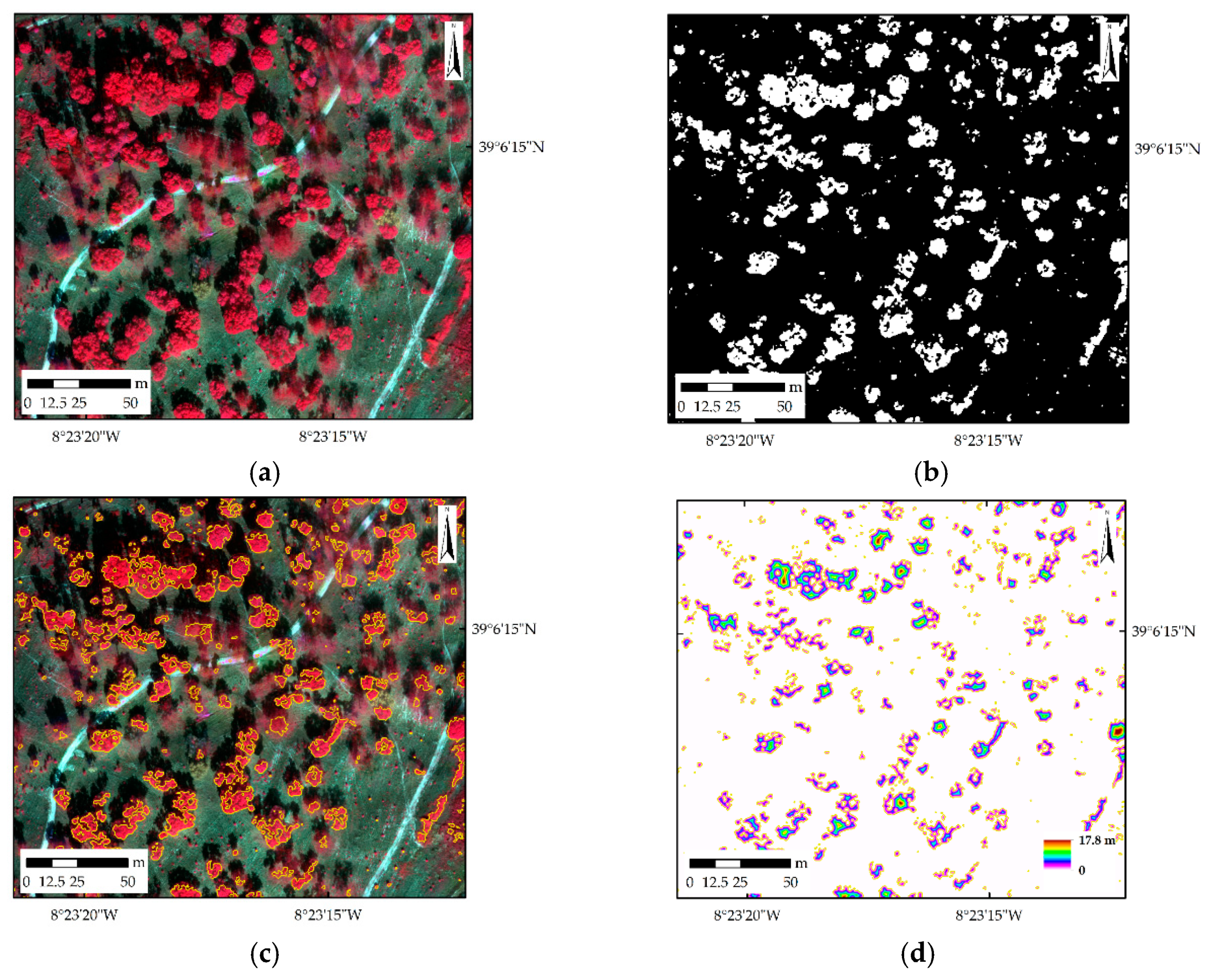
This algorithm works in two steps. In the first step, a locally adaptive threshold is applied based on the characteristics of the image’s grayscale values distribution to determine whether a given pixel is a tree or ground. This threshold is set based on the local mean intensity (local first-order statistics) in the neighbourhood of each pixel, separating the foreground from the background with nonuniform illumination. Grayscale images were resampled (downscaled) to 0.36 m and the size of the neighbourhood used to compute local statistic around each pixel was set as 11 × 11. A binary mask is then generated with the local mean threshold obtained from the original images (Figure 4b). However, this segmentation was not enough to segment individual tree crowns once several clusters of tree crowns are found in the image. Besides, some noise (e.g., clusters of a few pixels incorrectly identified as trees) was also present in the binary image. The next phase was to apply a low-pass filtering, using a 7 × 7 kernel size, in order to create a smoothing effect and therefore to remove noise. After noise removal, the binary image was converted into a polygon vector file with isolated trees and clusters of trees (Figure 4c). As the binary image defines the outer limit of tree crowns, polygons might have more than one tree and must be further analysed. This next step has the purpose of inferring the number of trees within each polygon and then the location of each tree. Polygons were first divided into two distinct sets depending on their area. Polygons with an area less or equal to 20 m2 were identified as isolated trees, while for the remaining polygons the Euclidean distance of the binary file was calculated (Figure 4d).
For each pixel in the binary file, a number corresponding to the distance between that pixel and the nearest zero pixel is assign. The maximum value for the Euclidean distance within each polygon was 25 pixels corresponding to 9 m (25 m × 0.36 m).
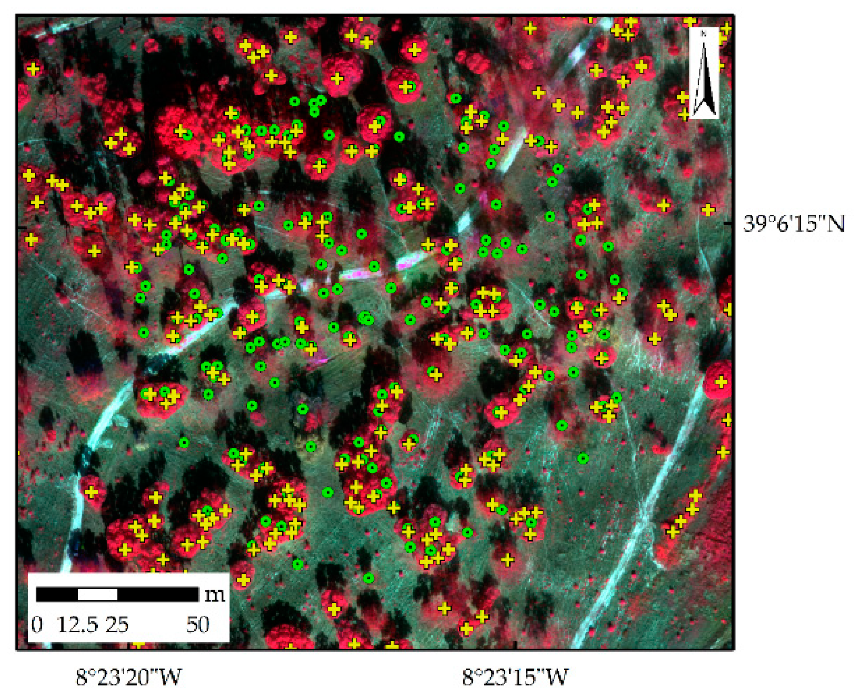
For the identification of each tree, the same strategy was adopted for both cases. Individual trees location was determined as the maximum of the distance function inside each isolated polygon, whilst in the case of tree clusters, the local maximum of the distance function was considered. In the latter case, local maximum values must exhibit a distance greater than the minimum distance between trees, set as 2 m. This is performed recursively for all local maximum of the distance function, beginning with the highest local maximum value. The result of the algorithm (Figure 5) is a file with the centroid of each tree crown that was validated using the location of the cork oak trees identified within the in situ data collection sites (150 m diameter circles).
2.7. Cork Oak Trees Spectral Characterisation and Temporal Variability
Cork oak decline is related with crown structure change due to leaf loss. This structural change may be detected using remote sensing data, which are able to interpret changes in green leaves and canopy structure.
First, reflectance values for all trees were extracted from the UAV and Sentinel-2 images considering the visible and the near infrared bands to evaluate the potential of the different spectral and spatial resolution data for the discrimination of healthy from unhealthy cork oak trees. This was performed just for one epoch as a first assessment of the cork oak vitality discriminant power of the Sentinel-2 images when compared with higher spatial resolution imagery.
Next, cork oak temporal variability was evaluated using several vegetation indices (VI) time series calculated from the Sentinel-2 images. The VI used in this study were the Normalised Difference Vegetation Index, NDVI [8], the Normalised Difference Water Index, NDWI [16], the Green Normalised Difference Vegetation Index, GNDVI [17] and the red-edge Chlorophyll Index, CI [18].
Common VI are based on red and near infrared spectral regions, however they usually saturate at moderate-to-dense canopies. Modified VIs, where the red/green spectral region is replaced with the red edge spectral region, are sensitive to chlorophyll content which depends on the physiological status of the plant. In the red edge region, there is an abrupt rise in the vegetation reflectance, from chlorophyll absorption in the red region to leaf cellular scattering in the near infrared region. So, the focus was in the comparison of red edge (chlorophyll) and visible and near infrared (structural) reflectance-based VI. Besides, replacing the red spectral region by the short-wave infrared (SWIR) spectral region, which reflects changes in the vegetation water content (water has high absorption in these wavelengths), makes NDWI a good indicator of plant water stress.
VI values were extracted based on the location of two separate sets of trees to generate the time series for the evaluation of the seasonal progression of cork oak phenological events. These two sets of trees were established based on the degree of defoliation: healthy trees with a percentage of defoliation less than 50% and unhealthy trees with a percentage of defoliation higher than 51%.
Besides the VI time series, the Vegetation Condition Index, VCI [19,20] and the temporal VI variability (mean and standard deviation as a ratio) were also considered (Equation 1). VCI is a NDVI pixel-wise normalization that is useful for making relative assessments by comparing the current NDVI to extreme NDVI values observed in the time series being analysed and is given by [21]:
where VIijk represents the monthly VI for pixel i in month j for year k, and VImax and VImin denote the multiyear minimum and maximum VI for pixel i. In this study, NDVI, CI, GNDVI and NDWI-derived VCI were computed based on the formula above replacing VI by NDVI, CI, GNDVI and NDWI, respectively.
In order to separate healthy from unhealthy trees a univariate analysis was performed. Thresholds for the spectral discrimination between the two cork oak classes were established by comparing the cumulative distribution function (CDF) for different VI time series. The CDF is a function derived from the probability density function for a random variable. It gives the probability of finding the random variable at a value less than or equal to a given cut-off (Equation (2)). For any random variable X, the CDF FX is defined as [22]:
which is the probability that X is less than or equal to x.
3. Results and Discussion
Cork oak trees locations obtained using the algorithm developed for the automatic tree crown identification based on very high-resolution UAV imagery were validated not only in terms of percentage of trees correctly identified but also in terms of positional accuracy. In situ measurements within the reference parcels were used to validate the results.
Preliminary visual analysis of both VI showed that, in the NDVI grayscale images, trees had a blurred appearance when compared to SAVI. The SAVI adequacy over the more popular NDVI in arid and semiarid zones, especially in medium spatial resolution, had already been reported by some authors [23,24]. Therefore, further developments of the algorithm were done based only on SAVI images.
Most of the tree crowns at site CL were correctly detected by the algorithm, whilst a slightly lower accuracy was verified for site HMG (Table 3). In the case of site CL, the number of tree crowns correctly detected corresponds to 85.4% of the trees in the validation dataset (140 out of 164 trees), while 4.2% (7 false positives) of the segmented crowns were detected erroneously. A slightly higher value of omitted tree crowns was obtained for site HMG, with 75.3% of tree being correctly detected, however in this case no false positives were verified. This lower overall accuracy might be justified not only by its rougher topography but also by a lower density of trees and a higher number of small trees.
Although the algorithm is still not able to fully under-segment individual trees in the presence of clusters of trees, denoting some dependence on the size and density of the trees, it proved to be useful for crown detection and delineation as compared to recent studies that employed high spatial resolution images [25]. Previous studies also reported that large and small crown density tends to be underestimated when optical images are used to delineate individual tree crowns [26]. Besides, Surový et al. [27] reported that cork oak crowns are more difficult to detect (higher omission errors), when compared to other types of trees with more regular crowns such as pine, due to their sparse canopy and lower density of leaves, especially in small trees.
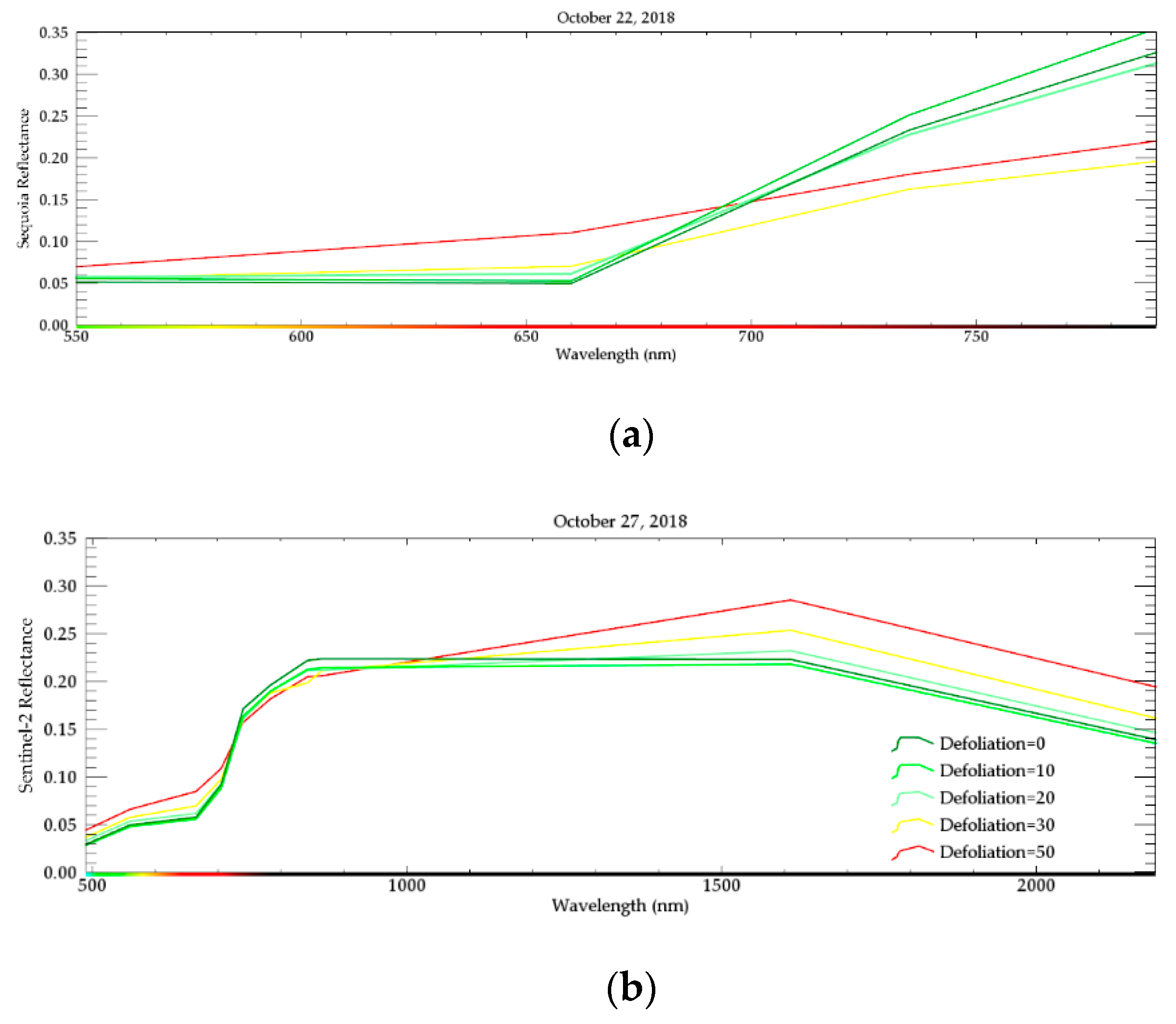
Both UAV and S2 spectral response (reflectance) for each defoliation class were analysed. In the case of the UAV images, only four spectral regions are available (green, red, red-edge and NIR), while for S2, all 10 and 20 m spatial resolution spectral regions, from blue (490 nm) to SWIR2 (2190 nm), were used. Figure 6a,b, show the spectral responses obtained, respectively, from the UAV and S2 images.
For the former case, one can observe that reflectance for trees with a defoliation degree higher than 50% or dead (defoliation classes 30 to 50, respectively) is significantly lower than the one observed for the other three classes (Figure 6a). Unhealthy trees show a slightly higher reflectance in the visible region, especially in the red band, and a significant lower reflectance in the red-edge and NIR bands in a UAV image acquired on 22 October 2018. Considering the S2 data acquired on 27 October 2018, the same spectral response is observed for the visible and NIR bands (Figure 6b). In the short-wave region (SWIR1 and SWIR2), unhealthy cork oak trees show a significantly higher reflectance, mainly for dead trees, when compared with healthy trees. This is an indicator that trees are subjected to water stress, once green vegetation spectra in the SWIR region is dominated by water absorption effects [28].
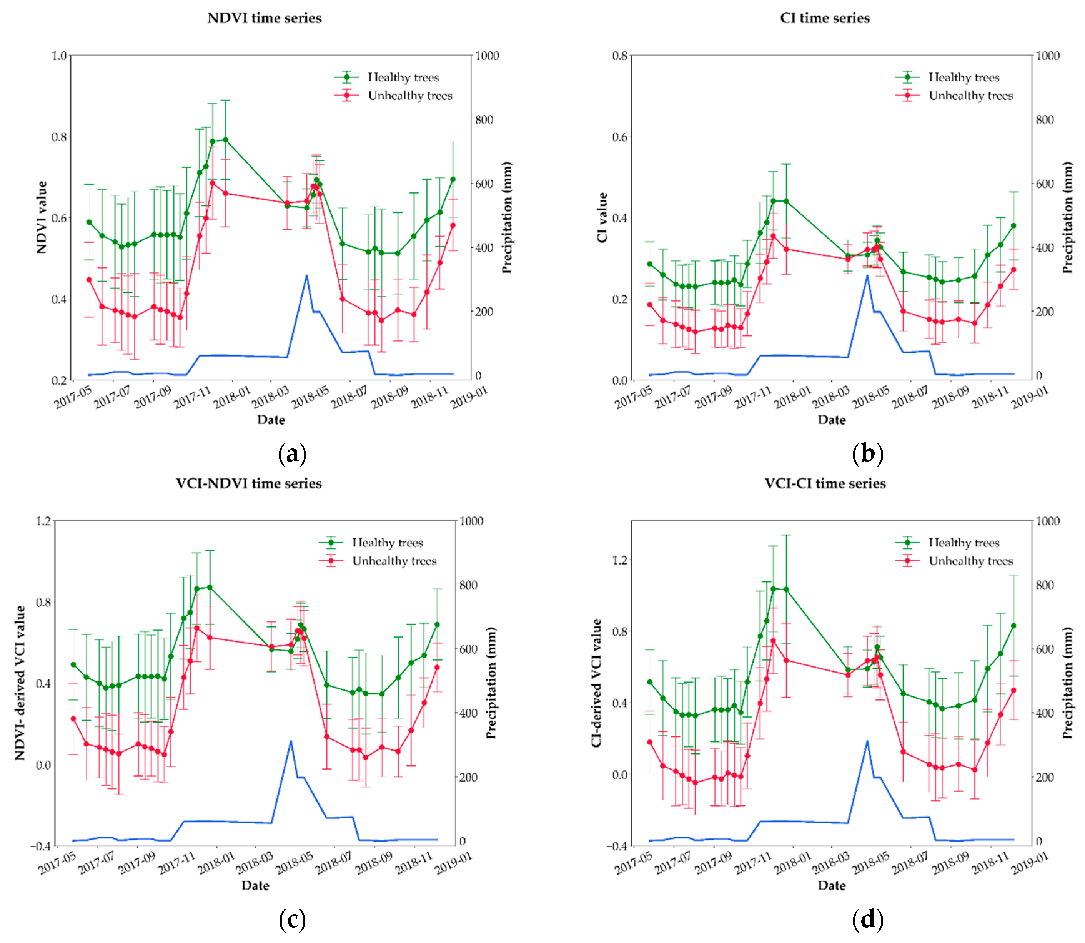
Regarding the VI time series analysis, results are very similar for all the indices considered in this study (Figure 7). The phenological behaviour of healthy and unhealthy trees is significantly distinct from July to October, while during winter months both exhibit almost the same behaviour. The performance of different VI, analysed by Dalponte et al. [26], was also very similar for dates that correspond to senescent background. Since unhealthy or dead trees show, respectively, little or absent photosynthetic activity, one can conclude that this increase in the VI values results from an increase in understory production due to precipitation, which in turn causes a significant contribution of the understory (or forest floor) spectral reflectance in the NIR region. As observed by some authors [29,30], NIR rapidly increases for sparse canopy covers when the understory starts sprouting after the first rains in October/November.
Healthy trees seem to be more resilient to the dry summer climate than the understory vegetation dominated by herbaceous vegetation and sparse shrubs, producing a higher contrast between tree crowns and ground. Precipitation data observed at a nearby weather station (Magos dam, 38°59′ N, 8°42′ W, 43 m in altitude) were superimposed to the NDVI time series in order to evaluate the relationship between rainfall and vegetation. During the dry season, there is a significant difference between the NDVI (and other VI) values for healthy and unhealthy trees, which fades when the rainy season begins (Figure 7a).
Based on indices calculated from in situ measurements with a FieldSpec 3 spectroradiometer, Cerasoli et al. [31] observed no correlation between rainfall and vegetation indices for cork oak, while a significant correlation was found for the herbaceous layer. This is not in line with our results, in which a positive correlation between rainfall and vegetation indices response was found, probably due to the low spatial resolution of the S2 images (10 m and 20 m), in which each pixel may include more than one tree as well as herbaceous vegetation. Nevertheless, there is a clear evidence that healthy cork oak trees behave differently than unhealthy trees over the year, with healthy trees exhibiting a lower VI temporal variability when compared to unhealthy trees. Therefore, the strategy is to define a threshold, allowing the separation between healthy and unhealthy trees, based on the temporal variability of cork oaks trees spectral response over one or more years.
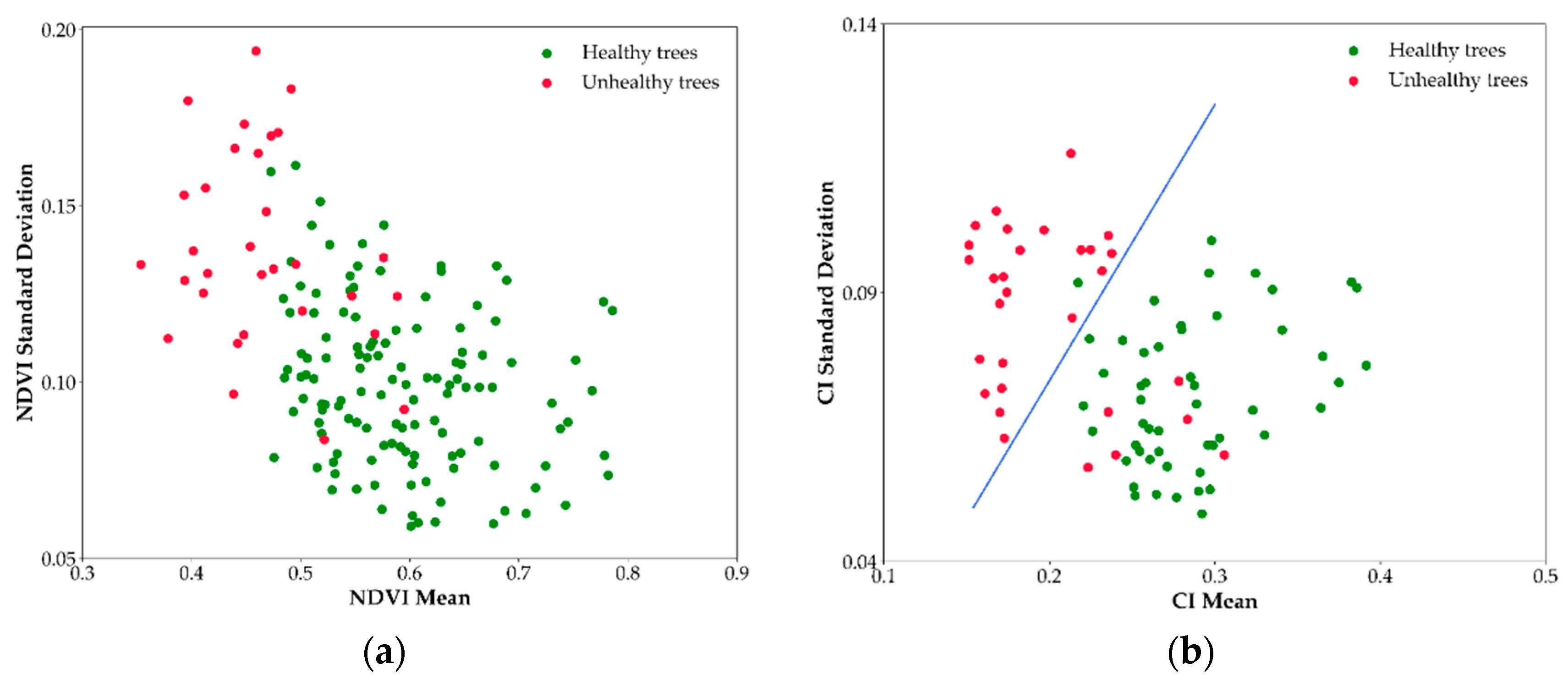
Analysis of the relationship between temporal mean and standard deviation for all VI indices allowed the evaluation of the temporal change rate for each tree using S2 data from 25 May 2017 to 6 December 2018. It is expected that healthy trees would have higher mean values and lower standard deviation values in opposition to unhealthy trees. This was verified by plotting the mean and standard deviation values for each tree obtained from each vegetation index time series. Best results were obtained when applying CI, enabling a clear separation between healthy and unhealthy trees with low omission and commission errors (Figure 8). As already observed by Zarco-Tejada et al. [13], the temporal change of rate of the CI vs. the NDVI made it possible to distinguish trees in healthy conditions from those undergoing decline, and moreover that it can potentially be used to define decline levels.
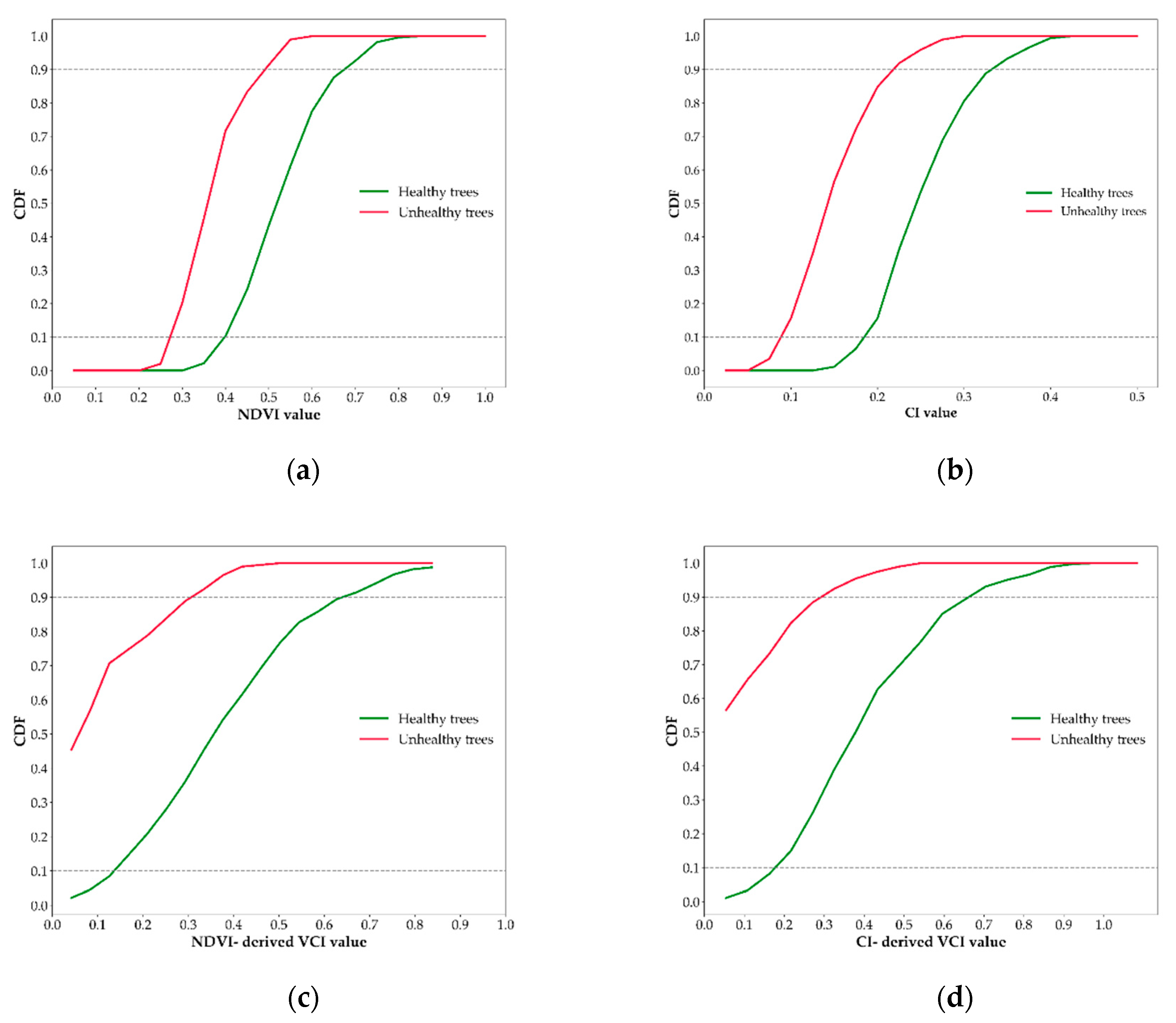
VCI was used as an indicator of the index dispersion for a certain epoch relatively to the temporal mean for a certain time series. VCI time series have a similar trend when compared with other VI time series, however, they seem to improve the discrimination between healthy and unhealthy cork oak trees. The separability between the two classes was objectively determined using the cumulative distribution function (CDF). The CDF function indicates the probability of finding a healthy (or unhealthy) cork oak for a given vegetation index value.
Figure 9 shows the cumulative distribution function for both classes of cork oaks considering NDVI and CI as well as the VCI associated with these indices for site HMG, NDVI, CI, and NDVI and CI-derived VCI values from September to October 2018 were used to define thresholds to separate healthy from unhealthy trees using a CDF. This time period was chosen since it corresponds to one of the periods along the year where the difference between the spectral responses of both cork oak classes is the highest. Thresholds were defined as the values for which the commission error for the class “unhealthy” is lower than a priori established value.
Considering a commission error of 10% (CDF = 0.1) for the class “unhealthy”, a value lower than 0.40 is obtained for the NDVI threshold (with an omission error of 34%), while a value lower than 0.18 is obtained for the CI threshold (with an omission error of 18%). Thus, in the latter case, 82% of unhealthy trees are correctly identified by considering CI values lower than 0.18, yet 10% of healthy trees are also classified as “unhealthy”. Likewise, for the same commission error, a value lower than 0.16 is obtained for the NDVI-derived VCI threshold (with an omission error of 25%), while a value lower than 0.10 is obtained for the CI-derived VCI threshold (with an omission error of 18%). Results for the CDF when using the VCI show a notorious discrimination between healthy and unhealthy cork oak trees.
The thresholds established for the identification of cork oak trees with vitality loss in site HMG were set as Equation (3):
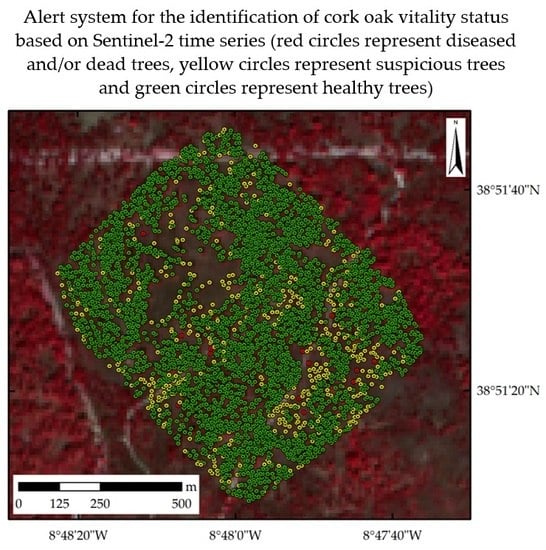
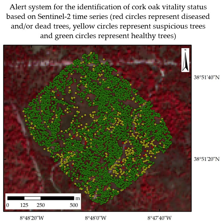
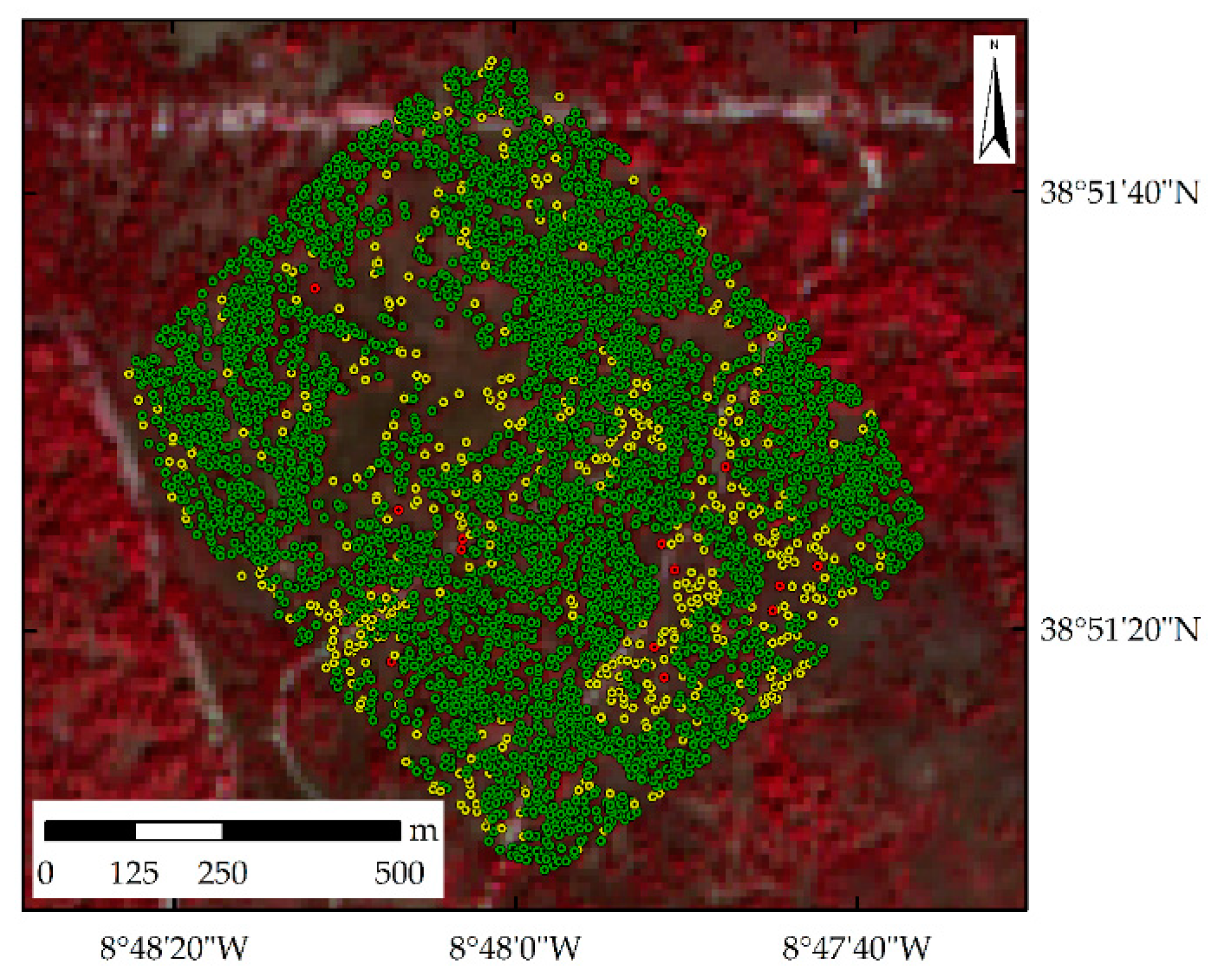
Based on these three conditions, an alert system was developed to provide information to the farmers on the location of potential diseased and/or dead trees. Cork oak trees that obey Equation (3) are considered by the system as highly probable diseased and/or dead tree (represented graphically as red circles on a vector file). Whenever any two conditions are verified simultaneously for a certain tree, this tree is highlighted as a suspicious tree (yellow circles), meaning that it is unclear if it is a real critical situation or an outlier resulting from the limitations of the S2 images spatial resolution. In the case of young trees (radius less than 2 m), the contribution from the understory within an area of 100 km2 is dominant when compared to a small-sized tree crown. All the remaining cork oak trees are considered by the system as healthy trees and, therefore, are represented as green circles.
To test the transferability of the method, these thresholds were applied to site CL using the same S2 time series. Figure 10 represents the results obtained when applying Equation (3) to site CL. These results were validated with defoliation data collected at the corresponding in situ data collection site. The total number of endangered trees identified by the alert system (in this case, 13) was slightly lower than the 19 unhealthy trees identified in the field. However, as already mentioned before, most of the cork oak trees identified incorrectly as diseased and/or dead, correspond to trees with small crowns.
4. Conclusions
A dense Sentinel-2 time series, covering a time period of around 18 months, was used to evaluate the potential of this free and open data for monitoring cork oak vitality. For this purpose, the temporal variability of two samples of healthy and unhealthy trees identified within the two in situ data collection sites considered in this study was analysed using different vegetation indices.
To focus the analysis at the tree level, very high-resolution UAV images were used to develop an algorithm for the automatic detection of individual trees. The algorithm relies first on the binary segmentation and filtering of a SAVI image, followed by an iterative method based on the Euclidean distance of the binary image to detect each tree centre. The algorithm was able to detect trees with an overall accuracy higher than 75%.
Independently of the vegetation index considered, cork oak status exhibited a positive correlation with increased precipitation for both sets of trees. During the rainy season, the increase in the spectral response of both types of trees in the near infrared region results from the spectral contribution of the understory to cork oak reflectance, particularly for trees with small crowns. However, during the dry season healthy cork oak trees showed higher spectral reflectance responses in the near infrared and red edge bands than unhealthy trees. This might be explained by the higher degree of defoliation exhibited by trees with loss of vitality, implying a reduced photosynthetic activity and consequently a lower spectral response in the near infrared region.
NDVI and CI were the vegetation indices that maximised the discrimination between healthy and unhealthy cork oak trees when using data corresponding to the driest period of 2018, which occurred from the beginning of September until the beginning of October. The ratio between the temporal mean and the temporal standard deviation calculated with data acquired during the dry season seems to be useful for the identification of cork oak trees with less vitality. Healthy cork oak trees showed higher NDVI and CI temporal mean values and lower temporal standard deviation values than unhealthy trees, which is easily explained by the fact that being an evergreen tree, its spectral response in the near infrared region is relatively stable along the year. Alternatively, the NDVI-derived VCI and CI-derived VCI also improved the discrimination between healthy and unhealthy cork oak trees when using a cumulative distribution function (CDF). Both approaches enabled the establishment of three simultaneous conditions for site HMG, which applied to the other test area (site CL) were able to detect around 68% of the unhealthy trees identified on the field.
These preliminary results seem promising, especially when considering VCI that is useful for making relative assessments of changes in the NDVI signal. Relative measurements of the present vegetation condition against a reference condition are critical for understanding and quantifying real vegetation conditions, characterized by historical mean.
Author Contributions
Conceptualization, J.C. (Joao Catalao) and A.N.; methodology, J.C. (Joao Catalao) and A.N.; software, J.C. (Joao Catalao) and J.C. (Joao Calvao); validation, J.C. (Joao Catalao) and A.N.; investigation, J.C. (Joao Catalao); writing—original draft preparation, A.N.; writing—review and editing, A.N., J.C. (Joao Catalao) and J.C. (Joao Calvao); supervision: J.C. (Joao Catalao).
Funding
This research was developed in the scope of the GEO SUBER project (PDR2020-101-031261) under the EU’s rural development policy that is funded through the European Agricultural Fund for Rural Development (EAFRD) from 2014 to 2020. The project is coordinated by the Portuguese Union of the Mediterranean Forest (UNAC)—PDR2020-101-031259. The publication is supported by FCT-project UID/GEO/50019/2019—Instituto Dom Luiz.
Acknowledgments
Authors acknowledge Herdade da Machoqueira do Grou and Companhia das Lezírias for allowing the access to the test sites and the use of the facilities. Authors would also like to thank Maria C. Caldeira (ISA), Conceição S. Silva (UNAC) and Systerra for providing data collected at the field in the scope of the GEO SUBER project.
Conflicts of Interest
The authors declare no conflict of interest. The funders had no role in the design of the study; in the collection, analyses, or interpretation of data; in the writing of the manuscript, or in the decision to publish the results.
References
- Uva, J.S. IFN6—Áreas Dos Usos Do Solo e Das Espécies Florestais de Portugal; Instituto da Conservação da Natureza e das Florestas: Lisboa, Portugal, 2013; p. 34. [Google Scholar]
- Godinho, S.; Guiomar, N.; Machado, R.; Santos, P.; Sá-Sousa, P.; Fernandes, J.P.; Neves, N.; Pinto-Correia, T.; Godinho, S.; Guiomar, Á.N.; et al. Assessment of Environment, Land Management, and Spatial Variables on Recent Changes in Montado Land Cover in Southern Portugal. Agrofor. Syst. 2016, 90, 177–192. [Google Scholar] [CrossRef]
- Costa, A.; Pereira, H.; Madeira, M. Analysis of Spatial Patterns of Oak Decline in Cork Oak Woodlands in Mediterranean Conditions. Ann. For. Sci. 2010, 67, 204. [Google Scholar] [CrossRef]
- Besson, C.K.; Lobo-Do-Vale, R.; Rodrigues, M.L.; Almeida, P.; Herd, A.; Grant, O.M.; Soares David, T.; Schmidt, M.; Otieno, D.; Keenan, T.F.; et al. Cork Oak Physiological Responses to Manipulated Water Availability in a Mediterranean Woodland. Agric. For. Meteorol. 2014, 184, 230–242. [Google Scholar] [CrossRef]
- Stocker, T.F.; Qin, D.; Plattner, G.K.; Tignor, M.M.B.; Allen, S.K.; Boschung, J.; Nauels, A.; Xia, Y.; Bex, V.; Midgley, P.M. Climate Change 2013 the Physical Science Basis: Working Group I Contribution to the Fifth Assessment Report of the Intergovernmental Panel on Climate Change; Cambridge University Press: Cambridge, UK, 2013. [Google Scholar] [CrossRef]
- Mendes, S.M.; Santos, J.; Freitas, H.; Sousa, J.P. Assessing the Impact of Understory Vegetation Cut on Soil Epigeic Macrofauna from a Cork-Oak Montado in South Portugal. Agrofor. Syst. 2011. [Google Scholar] [CrossRef]
- Tiberi, R.; Branco, M.; Bracalini, M.; Croci, F.; Panzavolta, T. Cork Oak Pests: A Review of Insect Damage and Management. Ann. For Sci. 2016. [Google Scholar] [CrossRef]
- Rouse, J.W.; Haas, R.H.; Schell, J.A.; Deeering, D. Monitoring Vegetation Systems in the Great Plains with ERTS (Earth Resources Technology Satellite). In Third Earth Resources Technology Satellite-1 Symposium; Freden, S.C., Mercanti, E.P., Becker, M.A., Eds.; NASA: Washington, DC, USA, 1973; pp. 309–317. [Google Scholar]
- Aubard, V.; Paulo, J.A.; Silva, J.M.N. Long-Term Monitoring of Cork and Holm Oak Stands Productivity in Portugal with Landsat Imagery. Remote Sens. 2019, 11, 525. [Google Scholar] [CrossRef]
- Santos, M.J.; Baumann, M.; Esgalhado, C. Drivers of Productivity Trends in Cork Oak Woodlands over the Last 15 Years. Remote Sens. 2016, 8, 486. [Google Scholar] [CrossRef]
- Modica, G.; Pollino, M.; Solano, F. Sentinel-2 Imagery for Mapping Cork Oak (Quercus suber L.) Distribution in Calabria (Italy): Capabilities and Quantitative Estimation. In Smart Innovation, Systems and Technologies; Verlag-Springer International Publishing: Cham, Switzerland, 2019. [Google Scholar] [CrossRef]
- Barnes, E.M.; Clarke, T.R.; Richards, S.E.; Colaizzi, P.D.; Haberland, J.; Kostrzewski, M.; Waller, P.; Choi, C.; Riley, E.; Thompson, T.; et al. Coincident Detection of Crop Water Stress, Nitrogen Status and Canopy Density Using Ground Based Multispectral Data. In Proceedings of the Fifth International Conference on Precision Agriculture, Bloomington, MN, USA, 16–19 July 2000. [Google Scholar]
- Zarco-Tejada, P.J.; Hornero, A.; Hernández-Clemente, R.; Beck, P.S.A. Understanding the Temporal Dimension of the Red-Edge Spectral Region for Forest Decline Detection Using High-Resolution Hyperspectral and Sentinel-2a Imagery. ISPRS J. Photogramm. Remote Sens. 2018. [Google Scholar] [CrossRef]
- APFC. Plano de Gestão Florestal Da Herdade Da Machoqueira Do Grou; Associação dos Produtores Florestais de Coruche (APFC): Coruche, Portugal, 2009. [Google Scholar]
- Huete, A.R. A Soil-Adjusted Vegetation Index (SAVI). Remote Sens. Environ. 1988. [Google Scholar] [CrossRef]
- Gao, B.C. NDWI—A Normalized Difference Water Index for Remote Sensing of Vegetation Liquid Water from Space. Remote Sens. Environ. 1996. [Google Scholar] [CrossRef]
- Gitelson, A.A.; Merzlyak, M.N. Signature Analysis of Leaf Reflectance Spectra: Algorithm Development for Remote Sensing of Chlorophyll. J. Plant Physiol. 1996. [Google Scholar] [CrossRef]
- Zarco-Tejada, P.J.; Miller, J.R.; Noland, T.L.; Mohammed, G.H.; Sampson, P.H. Scaling-Up and Model Inversion Methods with Narrowband Optical Indices for Chlorophyll Content Estimation in Closed Forest Canopies with Hyperspectral Data. IEEE Trans. Geosci. Remote Sens. 2001. [Google Scholar] [CrossRef]
- Kogan, F.N. Remote Sensing of Weather Impacts on Vegetation in Non-Homogeneous Areas. Int. J. Remote Sens. 1990. [Google Scholar] [CrossRef]
- Kogan, F.N. Application of Vegetation Index and Brightness Temperature for Drought Detection. Adv. Space Res. 1995. [Google Scholar] [CrossRef]
- Jiao, W.; Zhang, L.; Chang, Q.; Fu, D.; Cen, Y.; Tong, Q. Evaluating an Enhanced Vegetation Condition Index (VCI) Based on VIUPD for Drought Monitoring in the Continental United States. Remote Sens. 2016, 8, 224. [Google Scholar] [CrossRef]
- Math 105: Probability Module. Available online: https://blogs.ubc.ca/math105/discrete-random-variables/the-cumulative-distribution/ (accessed on 18 June 2019).
- Almutairi, B.; El Battay, A.; Belaid, M.A.; Musa, N. Comparative Study of SAVI and NDVI Vegetation Indices in Sulaibiya Area (Kuwait) Using Worldview Satellite Imagery. Int. J. Geosci. Geomat. 2013, 1, 50–53. [Google Scholar]
- Dos Santos, G.M.; Meléndez-Pastor, I.; Navarro-Pedreño, J.; Lucas, I. A Review of Landsat TM/ETM Based Vegetation Indices as Applied to Wetland Ecosystems. J. Geogr. Res. 2019, 2, 35–49. [Google Scholar]
- Wagner, F.H.; Ferreira, M.P.; Sanchez, A.; Hirye, M.C.M.; Zortea, M.; Gloor, E.; Phillips, O.L.; de Souza Filho, C.R.; Shimabukuro, Y.E.; Aragão, L.E.O.C. Individual Tree Crown Delineation in a Highly Diverse Tropical Forest Using Very High Resolution Satellite Images. ISPRS J. Photogramm. Remote Sens. 2018. [Google Scholar] [CrossRef]
- Dalponte, M.; Ørka, H.O.; Ene, L.T.; Gobakken, T.; Næsset, E. Tree Crown Delineation and Tree Species Classification in Boreal Forests Using Hyperspectral and ALS Data. Remote Sens. Environ. 2014. [Google Scholar] [CrossRef]
- Surový, P.; Almeida Ribeiro, N.; Panagiotidis, D. Estimation of Positions and Heights from UAV-Sensed Imagery in Tree Plantations in Agrosilvopastoral Systems. Int. J. Remote Sens. 2018. [Google Scholar] [CrossRef]
- Sánchez-Ruiz, S.; Piles, M.; Sánchez, N.; Martínez-Fernández, J.; Vall-llossera, M.; Camps, A. Combining SMOS with Visible and near/Shortwave/Thermal Infrared Satellite Data for High Resolution Soil Moisture Estimates. J. Hydrol. 2014. [Google Scholar] [CrossRef]
- Häusler, M.; Silva, J.M.N.; Cerasoli, S.; López-Saldaña, G.; Pereira, J.M.C. Modelling Spectral Reflectance of Open Cork Oak Woodland: A Simulation Analysis of the Effects of Vegetation Structure and Background. Int. J. Remote Sens. 2016. [Google Scholar] [CrossRef]
- Ramos, A.; Pereira, M.J.; Soares, A.; Do Rosário, L.; Matos, P.; Nunes, A.; Branquinho, C.; Pinho, P. Seasonal Patterns of Mediterranean Evergreen Woodlands (Montado) Are Explained by Long-Term Precipitation. Agric. For. Meteorol. 2015. [Google Scholar] [CrossRef]
- Cerasoli, S.; Costa e Silva, F.; Silva, J.M.N. Temporal Dynamics of Spectral Bioindicators Evidence Biological and Ecological Differences among Functional Types in a Cork Oak Open Woodland. Int. J. Biometeorol. 2016. [Google Scholar] [CrossRef]
Figure 1.
(a) Test sites location (white dots) approximately 50 km (CL) and 100 km (HMG) northeast of Lisbon; (b) Companhia das Lezírias (CL) and (c) Herdade da Machoqueira do Grou (HMG). Yellow polygons represent the limits of the test sites and yellow triangles the location of the ground control points (CGPs).

Figure 2.
Location of the cork oak trees (green circles) considered for in situ measurements in Herdade da Machoqueira do Grou (HMG).
Figure 2.
Location of the cork oak trees (green circles) considered for in situ measurements in Herdade da Machoqueira do Grou (HMG).

Figure 3.
In situ photos of GCP used to rectify the UAV imagery.

Figure 4.
HMG test site: (a) False-colour composite image (NIR, R, G); (b) Binary image with the tree crowns (in white); (c) tree crown´s delimitation (in yellow) superimposed on the false-colour composite; and (d) Euclidean distance calculated from the binary image.
Figure 4.
HMG test site: (a) False-colour composite image (NIR, R, G); (b) Binary image with the tree crowns (in white); (c) tree crown´s delimitation (in yellow) superimposed on the false-colour composite; and (d) Euclidean distance calculated from the binary image.

Figure 5.
Individual tree location obtained using the developed algorithm (yellow cross) and coordinated at the field (green circles) for site HMG.
Figure 5.
Individual tree location obtained using the developed algorithm (yellow cross) and coordinated at the field (green circles) for site HMG.

Figure 6.
(a) Spectral response of cork oak trees with a defoliation degree <50% (green lines) and with a defoliation degree >51% or dead (yellow and red lines) for the HMG test sites using an UAV image collected at October 22 2018; (b) spectral response of cork oak trees with a defoliation degree <50% (green lines) and with a defoliation degree >51% or dead (yellow and red lines) for the HMG test sites using S2 image collected at October 27 2018 (no tree was classified as defoliation class 40 in this test site).

Figure 7.
Healthy (green) and unhealthy (red) cork oak trees temporal variability computed based on the NDVI (a), CI (b), NDVI-derived VCI (c), and CI-derived VCI (d) indices. Monthly precipitation values (blue line), obtained from the Magos Dam weather station, are superimposed to the NDVI time series calculated for the HMG test site.

Figure 8.
Relationship between NDVI (a) and CI (b) temporal mean and temporal standard deviation for the HMG test site (green circles correspond to healthy trees while red circles correspond to unhealthy trees).
Figure 8.
Relationship between NDVI (a) and CI (b) temporal mean and temporal standard deviation for the HMG test site (green circles correspond to healthy trees while red circles correspond to unhealthy trees).

Figure 9.
Cumulative distribution function (CDF) applied to NDVI (a), CI (b), NDVI-derived VCI (d), and CI-derived VCI (d) for site HMG. Green lines show the cumulative probability of healthy trees while red lines show the cumulative probability of unhealthy trees.
Figure 9.
Cumulative distribution function (CDF) applied to NDVI (a), CI (b), NDVI-derived VCI (d), and CI-derived VCI (d) for site HMG. Green lines show the cumulative probability of healthy trees while red lines show the cumulative probability of unhealthy trees.

Figure 10.
Results of the alert system for site CL (red circles represent diseased and/or dead trees, yellow circles represent suspicious trees and green circles represent healthy trees) superimposed to a S2 false-coloured composite.
Figure 10.
Results of the alert system for site CL (red circles represent diseased and/or dead trees, yellow circles represent suspicious trees and green circles represent healthy trees) superimposed to a S2 false-coloured composite.


Table 1.
Image’s acquisition dates (Sentinel-2 Level-2A images and UAV images).
| Month/Year | Mar | Apr | May | Jun | Jul | Aug | Sep | Oct | Nov | Dec | |
|---|---|---|---|---|---|---|---|---|---|---|---|
| Sentinel-2 | 2017 | 25 | 14 | 4 14 24 | 3 | 2 12 22 | 2 12 22 | 11 21 | 1 21 | ||
| 2018 | 26 | 25 | 5 10 15 | 19 | 29 | 8 18 | 12 | 7 27 | 16 | 6 | |
| UAV/HMG | 2018 | 26 | 22 | ||||||||
| UAV/CL | 12 | 23 |
Table 2.
The degree of defoliation by cork oak class considered in this study.
| Defoliation Class | Percentage of Defoliation | Tree Status |
|---|---|---|
| 0 | 0–10% | Healthy |
| 10 | 11–25% | Healthy |
| 20 | 26–50% | Healthy |
| 30 | 51–90% | Unhealthy |
| 40 | >90% | Unhealthy |
| 50 | Dead tree | Unhealthy |
Table 3.
Omission and commission error of the automatic tree crown identification.
| Omission | Commission | Accuracy | |
|---|---|---|---|
| CL | 24/164 | 7/164 | 85% |
| HMG | 45/182 | 0/182 | 75% |
© 2019 by the authors. Licensee MDPI, Basel, Switzerland. This article is an open access article distributed under the terms and conditions of the Creative Commons Attribution (CC BY) license (http://creativecommons.org/licenses/by/4.0/).
Share and Cite
MDPI and ACS Style
Navarro, A.; Catalao, J.; Calvao, J. Assessing the Use of Sentinel-2 Time Series Data for Monitoring Cork Oak Decline in Portugal. Remote Sens. 2019, 11, 2515. https://0-doi-org.brum.beds.ac.uk/10.3390/rs11212515
AMA Style
Navarro A, Catalao J, Calvao J. Assessing the Use of Sentinel-2 Time Series Data for Monitoring Cork Oak Decline in Portugal. Remote Sensing. 2019; 11(21):2515. https://0-doi-org.brum.beds.ac.uk/10.3390/rs11212515
Chicago/Turabian StyleNavarro, Ana, Joao Catalao, and Joao Calvao. 2019. "Assessing the Use of Sentinel-2 Time Series Data for Monitoring Cork Oak Decline in Portugal" Remote Sensing 11, no. 21: 2515. https://0-doi-org.brum.beds.ac.uk/10.3390/rs11212515
Note that from the first issue of 2016, this journal uses article numbers instead of page numbers. See further details here.