First Evaluation of Topography on GNSS-R: An Empirical Study Based on a Digital Elevation Model


Centre Tecnòlogic de Telecomunicacions de Catalunya (CTTC/CERCA), 08860 Castelldefels (Barcelona), Spain
*
Author to whom correspondence should be addressed.
Remote Sens. 2019, 11(21), 2556; https://0-doi-org.brum.beds.ac.uk/10.3390/rs11212556
Submission received: 16 September 2019
/
Revised: 11 October 2019
/
Accepted: 29 October 2019
/
Published: 31 October 2019
(This article belongs to the Special Issue Applications of GNSS Reflectometry for Earth Observation)
Abstract
:Understanding the effects of Earth’s surface topography on Global Navigation Satellite Systems Reflectometry (GNSS-R) space-borne data is important to calibrate experimental measurements, so as to provide accurate soil moisture content (SMC) retrievals. In this study, several scientific observables obtained from delay-Doppler maps (DDMs) generated on board the Cyclone Global Navigation Satellite System (CyGNSS) mission were evaluated as a function of several topographic parameters derived from a digital elevation model (DEM). This assessment was performed as a function of Soil Moisture Active Passive (SMAP)-derived SMC at grazing angles ~ [20,30] ° and in a nadir-looking configuration ~ [80,90] °. Global scale results showed that the width of the trailing edge (TE) was small ~ [100, 250] m and the reflectivity was high ~ [–10, –3] dB over flat areas with low topographic heterogeneity, because of an increasing coherence of Earth-reflected Global Positioning System (GPS) signals. However, the strong impact of several topographic features over areas with rough topography provided motivation to perform a parametric analysis. A specific target area with little vegetation, low small-scale surface roughness, and a wide variety of terrains in South Asia was selected. A significant influence of several topographic parameters i.e., surface slopes and curvatures was observed. This triggered our study of the sensitivity of and to SMC and topographic wetness index (). Regional scale results showed that and are strongly correlated with the , while the sensitivity to SMC was almost negligible. The Pearson correlation coefficients of and with are ~ 0.59 and ~−0.63 at ~ [20, 30] ° and ~ 0.48 and ~ −0.50 at ~ [80, 90] °, respectively.
1. Introduction
Soil moisture content (SMC) is an important component in the global water and energy balance because it determines the flux of water that infiltrates to groundwater or drains via surface water [1]. SMC determines the water and energy available for evapotranspiration. The dependence of SMC on topographic convergence suggests that topography is an important element in the spatial distribution of SMC [2]. The state and pattern of SMC affect the hydrological response of a catchment area [1]. Temporal dynamics in the state of SMC depend on rates of outgoing horizontal and vertical fluxes, e.g., drainage and evaporation. On the other hand, the dependence of SMC on topographic convergence [2] suggests that topography is an important factor that partially determines the spatial distribution of SMC. As such, processes that lead to spatial organization in SMC could be represented by topographic parameters derived from a digital elevation model (DEM). Indeed, topography-based wetness indices can be used to predict the spatial distribution of wetlands because topography is one of the most important elements that influences the spatial patterns of saturated areas. Alternatively, wetlands mapping and spatial patterns of wetness can be generated in catchments under the assumption that groundwater tables follow topography holds.
The future of Earth observation in SMC determination is strongly based on the ability of the next generation of space-borne sensors to improve the Earth’s surface spatio-temporal sampling properties. Global Navigation Satellite Systems Reflectometry (GNSS-R) appears in this framework, with an intrinsic capability to advance over more classical remote sensing approaches. GNSS-R is a sort of L-band passive bistatic radar (as many transmitters as navigation satellites are in view) that provides a wide swath up to ~ 1500 km. It was first conceived as an interferometric technique or iGNSS-R to provide higher precision in ocean altimetry measurements [3,4]. However, it can also be used for land surfaces applications. In this scenario, the conventional GNSS-R technique or cGNSS-R is more appropriate because lower coherent and incoherent integration times are required, so that the associated spatial resolution is improved [5]. At present, several works have demonstrated the feasibility of SMC estimation using space-borne cGNSS-R data from the United Kingdom (U.K.) TechDemoSat-1 [6,7,8], Soil Moisture Active Passive (SMAP) [9], and Cyclone Global Navigation Satellite System (CyGNSS) [10,11] missions.
CyGNSS was selected by the National Aeronautics and Space Administration (NASA) in 2012 as a highly innovative Earth Venture space system, and it was launched into space on 15 December 2016 [12]. CyGNSS is an 8-microsatellite constellation. Each single CyGNSS satellite carries on board two down-looking antennas with left hand circular polarization (LHCP). Both antennas point to the Earth’s surface with an elevation angle ~ 62 ° on each side of the satellite ground track ( ~ 90 °at the normal direction to the Earth’s surface). The gain of the antennas is ~ 14.7 dB (antenna boresight).
Topographic inhomogeneities can distort GNSS-R measurements [13,14]. They have to be compensated to improve the accuracy in the retrieval of SMC. In a bistatic radar geometry, GNSS scattered signals can be collected along the specular direction (elevation angle of the incident wave equals elevation angle of the scattered wave i.e., ==). The scattering is only strong over an area around the nominal specular point. On the other hand, the scattering area depends on the local topography as well as on the GNSS satellites’ elevation angles. Local slopes modify the scattering area as compared to that corresponding to a flat Earth assumption. The scattering area may be a complex and sometimes non-contiguous area on ground. However, it remains uncertain to what extent topography influences GNSS-R data and how these effects can be corrected. The main purpose of the present investigation was to further understand the effects of rough topography using data collected by CyGNSS. The counterpart of the radar pulse width in CyGNSS is ~ 300 m (1 C/A code chip). As such, reflected delay Doppler maps (DDMs) are potentially sensitive to the relative orientation of the scattering surfaces, but also to the vertical relief distribution. In the first part of this study, the influence of six different topographic parameters derived from the Global Multi-resolution Terrain Elevation Data 2010 (GMTED2010) model on DDMs derived from CyGNSS Level 1 Science Data Record Version 2.1 [12,15,16] was evaluated as a function of SMC derived from SMAP-enhanced L3 Radiometer Global Daily 9 km Level L3 SPL3SMP_E Version 1.0 product. In the last part, the following question was addressed: Can topographic features determine the main spatial pattern of Earth’s surface reflectivity as it is measured by CyGNSS?
The remainder of this paper is organized as follows. Section 2 provides a theoretical background on the effects of topography on GNSS-R. Section 3 describes the methodology. Section 4 describes the effects of topography on CyGNSS-derived DDMs based on several parameters derived form a DEM. Additionally, it investigates the relationship between DDMs and a topography-based surface wetness index. Section 5 includes final discussions, and the main conclusions are discussed in Section 6.
2. Theoretical Background
CyGNSS allows sampling of the Earth’s surface along 32 tracks simultaneously, within a wide range of satellites’ elevation angles ~ [20, 90] ° over the tropical latitudinal band Latitude ~ [−40, 40]°. Geophysical parameters retrieval from CyGNSS requires that the GNSS-R payload cross-correlates directly the collected signals against a known replica of the GPS L1 C/A code, after compensating for the Doppler shift. Consequently, 32 complex reflected DDMs,, are generated on board at a time, using a short coherent integration time,~ 1 ms. Complex DDMs, , are incoherently averaged along ~ 1 s to finally generate the so-called power DDMs.
Power DDMs, , can be modelled using geometrical and scattering related parameters as follows [17]:
where is the power of the right HCP(RHCP) transmitted signals, ~ 19 cm is the wavelength of the signals at L1, and are the transmitting and receiving antenna gains, and are the ranges from the transmitter and the receiver to the specular point, respectively, is the Woodward ambiguity function (WAF), is the delay of the signal from the transmitter to the receiver, is the Doppler shift of the reflected signal, is aimed to compensate the Doppler shift of the signal, is the bistatic scattering coefficient at LHCP, and is the positioning vector of the scattering point.
The bistatic scattering coefficient can be defined as follows [18]:
where and are the coherent and the incoherent scattering terms respectively. Consequently, DDMs consist on a sum of two terms as follows [19,20,21]:
accounts for coherent reflections from the surface, while is responsible for the diffuse scattering.
can be expressed analytically as follows [10]:
where is the LHCP Fresnel reflection coefficient, is the signal angular wavenumber, is the surface height standard deviation (related to small-scale surface roughness), and is the transmissivity of the vegetation.
includes contributions from vegetation, small-scale surface roughness, and topography. Further details on the incoherent scattering over rough surfaces can be found in Reference [22]. The impact of vegetation should be also considered to establish a model of the incoherent scattered field. A comprehensive method can be found in References [23,24].
Over regions without rough topography, DDMs can be expressed as follows [25]:
where is the 2-D convolution in both domains, delay and Doppler. The WAF can be defined as follows [17]:
where is the autocorrelation function of the pseudo-random noise (PRN) codes and is the system impulse response in the frequency domain.
Regions with rough topography are characterized with a root mean square error (RMSE) of the surface height variation higher than the length of the GNSS code under study. The effects of rough topography in the DDMs can be understood as follows:
where the function represents the mean density of scattering points as a function of the delay, and the Doppler shift.
3. Data and Methodology
3.1. Topographic Parameters
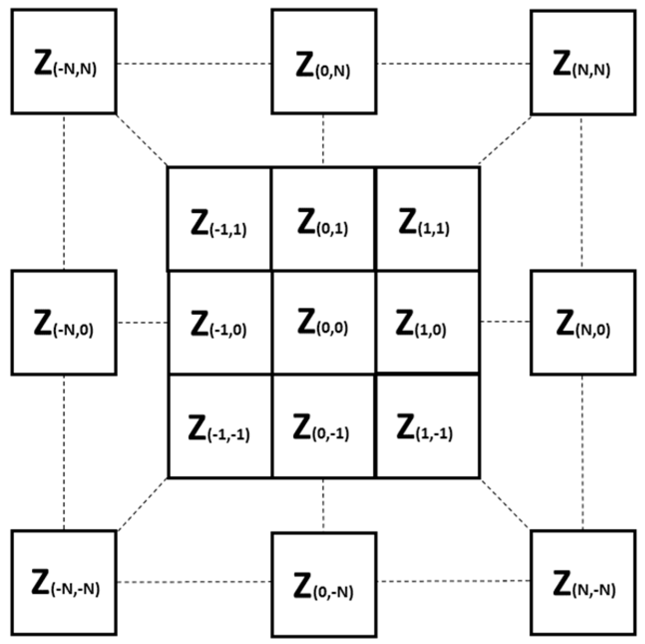
Several topographic parameters were derived from the ~250 m GMTED2010 model based on a 3 × 3 moving window (Figure 1). This window was composed of the focal cell and its eight surrounding cells. The DEM surface was approximated by a bivariate quadratic equation [26,27]:
where represents the height of the DEM surface and and are the horizontal coordinates. The coefficients in Equation (8) were solved within the 3 × 3 window using simple combinations of neighboring cells, based on the so-called Wood’s approach [28].
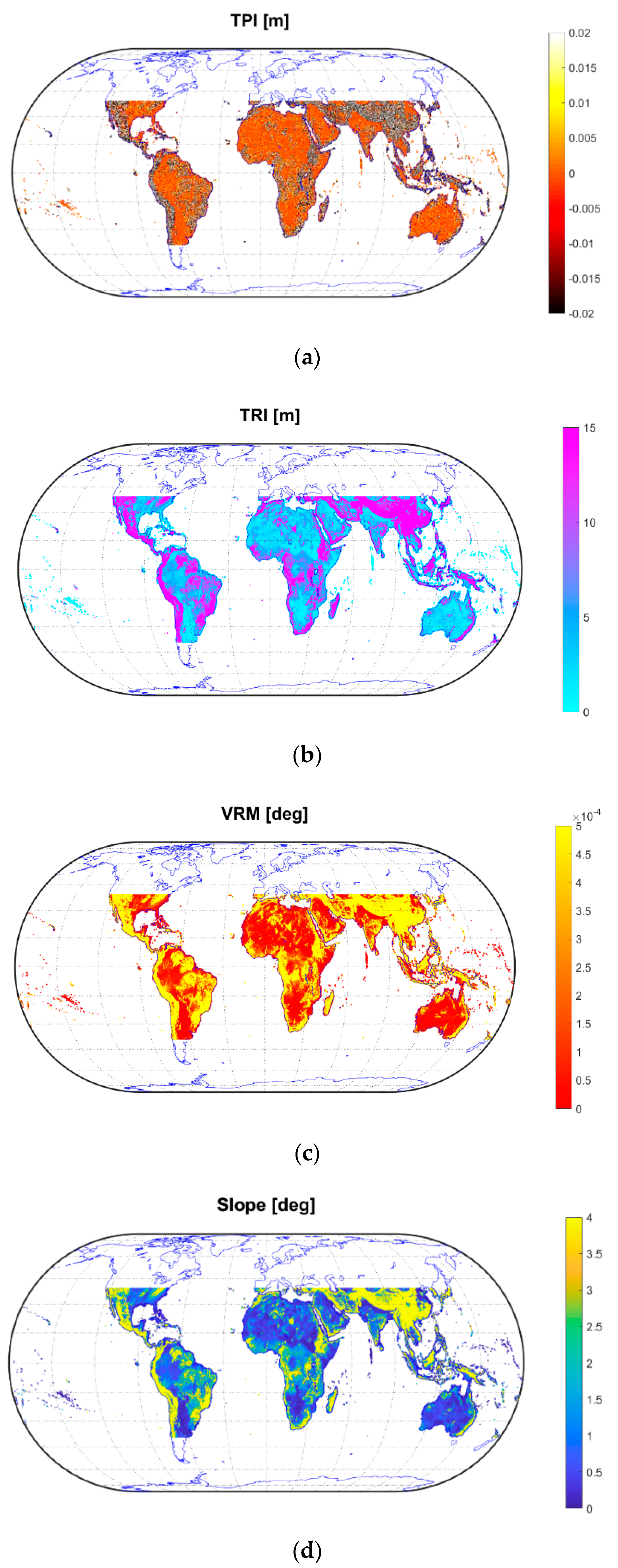
The topographic parameters were used to investigate the impact of different topographic features on . In particular, three heterogeneity variables (topographic position index or , terrain ruggedness index or , vector ruggedness measure or ), slope (), and two curvature variables (tangential () and profile curvature () were used in the parametric study. They have the potential to enable a better understanding on the properties of the Earth’s surface than raw DEM data. Topographic heterogeneity is described as the variability of surface elevations within an area. On the other hand, curvature attributes are based on the change of slope in a particular direction. More specifically, the selected topographic parameters (Figure 2) were defined as follows [26,27,28]:
- is the difference between the elevation of a focal cell and the mean of its eight surrounding cells. Positive and negative values correspond to ridges and valleys, respectively. Zero values correspond to flat areas. It was computed as follows:where is total number of surrounding points employed in the evaluation.
- is the mean of the absolute differences in elevation between a focal cell and its eight surrounding cells. It quantifies the total elevation change across the 3 × 3 moving window. Flat areas have a value of zero and mountain areas with steep ridges have positive values. It was computed as follows:where and may be any odd integer smaller than the number of cells in the shortest side of the raster.
- quantifies the terrain ruggedness based on the measurements of the dispersion of vectors orthogonal to the surface. VRM quantifies the local variation of slope in the terrain more independently than TPI and TRI. VRM values range from 0 over flat areas to 1 over rough areas. It was computed using vector analysis [26].
- is defined as the rate of change of elevation in magnitude for the steepest descent vector. It influences hydraulic gradients driving any surface flows and also sub-surface flows when the water table has a similar slope to the ground surface. Slope and curvature serve as useful input variables in erosion and hydrological models. It was computed as follows:
- measures the rate of change perpendicular to the slope gradient. It is related to the convergence and divergence of lateral flows across a surface. It was computed as follows:
- measures the rate of change of slope along a flow line. It affects the acceleration or deceleration of surface flows along the surface and thus it influences erosion and deposition of soils. Positive and negative values indicate convex and concave surfaces, respectively. It was computed as follows:
3.2. Topographic Wetness Index
The topographic wetness index () is a parameter used to match runoff- producing elements in the landscape [29]. Different target areas with similar values should have similar hydrological dynamics [30]. As such, is an indicator of the relative propensity of soils to become saturated to the surface because of the local topography. In this work, values were calculated based on the GA2 algorithm [31]. GA2 calculates the outflow gradient of each target area and uses precalculated up-land values from HydroSHEDS for the catchment area [32]. It can be expressed as follows [31]:
where is the specific catchment area [33,34]. values are low at ridges and high in valleys. Generally, humid areas generate higher values, although there are some exceptions such as desert areas where high values do not correlate with high flow accumulation.
3.3. Delay Doppler Maps Parameters
CyGNSS Level 1 Science Data Record Version 2.1 [12,15,16] was selected for this study. Original data were first filtered out using an equivalent “CyGNSS overall quality flag” over land surfaces [35]. Reflected delay waveforms were obtained from the original DDMs at zero Doppler frequency:
The delay bin resolution of the original 17 lag waveforms was ~ 0.2552 GPS C/A chips. A re-sampling and interpolation of the resulting 1700 lag waveforms was performed using a spline method to increase the accuracy of the waveforms, before applying the algorithms to extract the observables.
The trailing edge (TE) width was defined as the lag difference between the 70% power threshold of the high resolution waveforms , and that corresponding to the maximum power of the waveforms [9]:
Different power thresholds were tested. The 50% power threshold was found to cut off some lags, when this threshold was out of the original 17 lag waveforms. On the other hand, the 90% power threshold provided a lower dynamic range as compared to the 70%. The incoherent scattering term was the main contribution to , while both the coherent and the incoherent scattering terms significantly contributed to the peak power of the waveforms .
The reflectivity was estimated as the ratio of the reflected and the direct power waveforms’ peaks, after compensating for the noise power floor and the antennas’ gain patterns as a function of the elevation angle as in [10]:
The antennas’ gain patterns were compensated versus the gain at the corresponding boresight direction, and the difference of both antennas at boresight [10]. The nominal mission lifetime was 2 years. This milestone was achieved in March 2019. At present, the mission is operating nominally, and the automatic gain control (AGC) was disabled from August 2018 [12]. This fact improves the accuracy in the estimation of using Equation (17). On the other hand, could also be inverted from scattering models. This approach relies on the assumption that the scattering is totally coherent [35] or totally incoherent [36]. The assumption in [35] is valid over smooth surface areas with little vegetation. The assumption in [36] is valid if inland water bodies are removed. However, in a more general scenario, the total scattered electromagnetic field is composed of both a coherent and an incoherent contribution [18] in different proportions depending on the dielectric and geometrical properties of the scattering medium, and the directions of incoming and outgoing electromagnetic waves. Both, the coherent and the incoherent scattering terms contribute to the peak power of the waveforms. This was the main motivation to use Equation (17) in this work.
4. Understanding the Effects of Rough Topography on GNSS-R Space-Borne Data
4.1. Global Scale
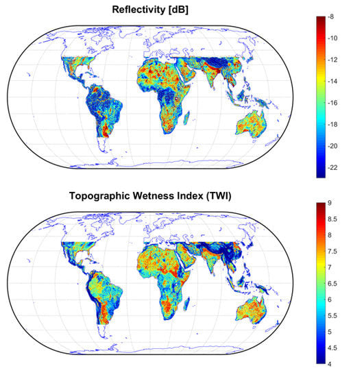
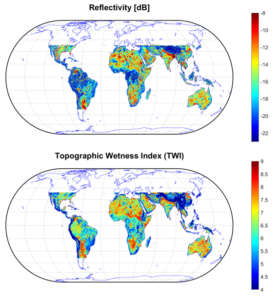
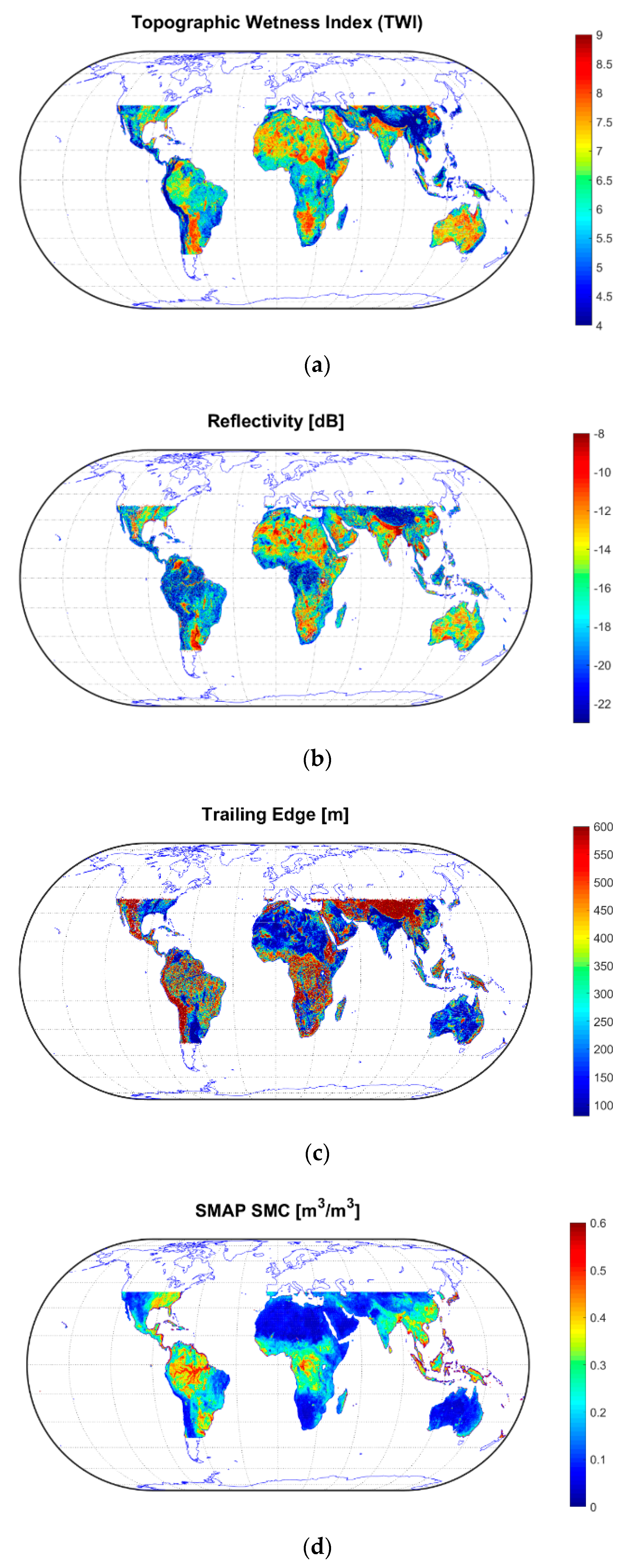
The main goal of this work was to study the impact of rough topography on CyGNSS-derived & as a function of SMAP-derived SMC. As a first step, the selected topographic parameters (Figure 2), (Figure 3a), CyGNSS-derived and (Figure 3b,c), and SMAP-derived SMC (Figure 3d) were displayed over the complete coverage of the Earth’s surface enabled by CyGNSS. SMC data were derived based on the V-pol single channel algorithm [37,38]. Corrections for roughness, effective surface temperature, and vegetation water content (VWC) were also applied. Six months of CyGNSS and SMAP data were selected from 1 August 2018 to 31 January 2019. This specific time period was selected because the AGC was disabled in July 2018, so as to improve the performance in the estimation of (Equation (17)). The selected temporal length was as large as possible at the time of starting this work. All the parameters were averaged using a 0.1° × 0.1° latitude/longitude grid with a moving window of 0.2° in steps of 0.1°. This gridding strategy enabled the analysis using auxiliary data and different sensors. The resulting spatial resolution was ~ 20 km × ~ 20 km at equatorial latitudes, which was wide enough to account for the across-track spreading ~ 20 km of the DDMs due to .
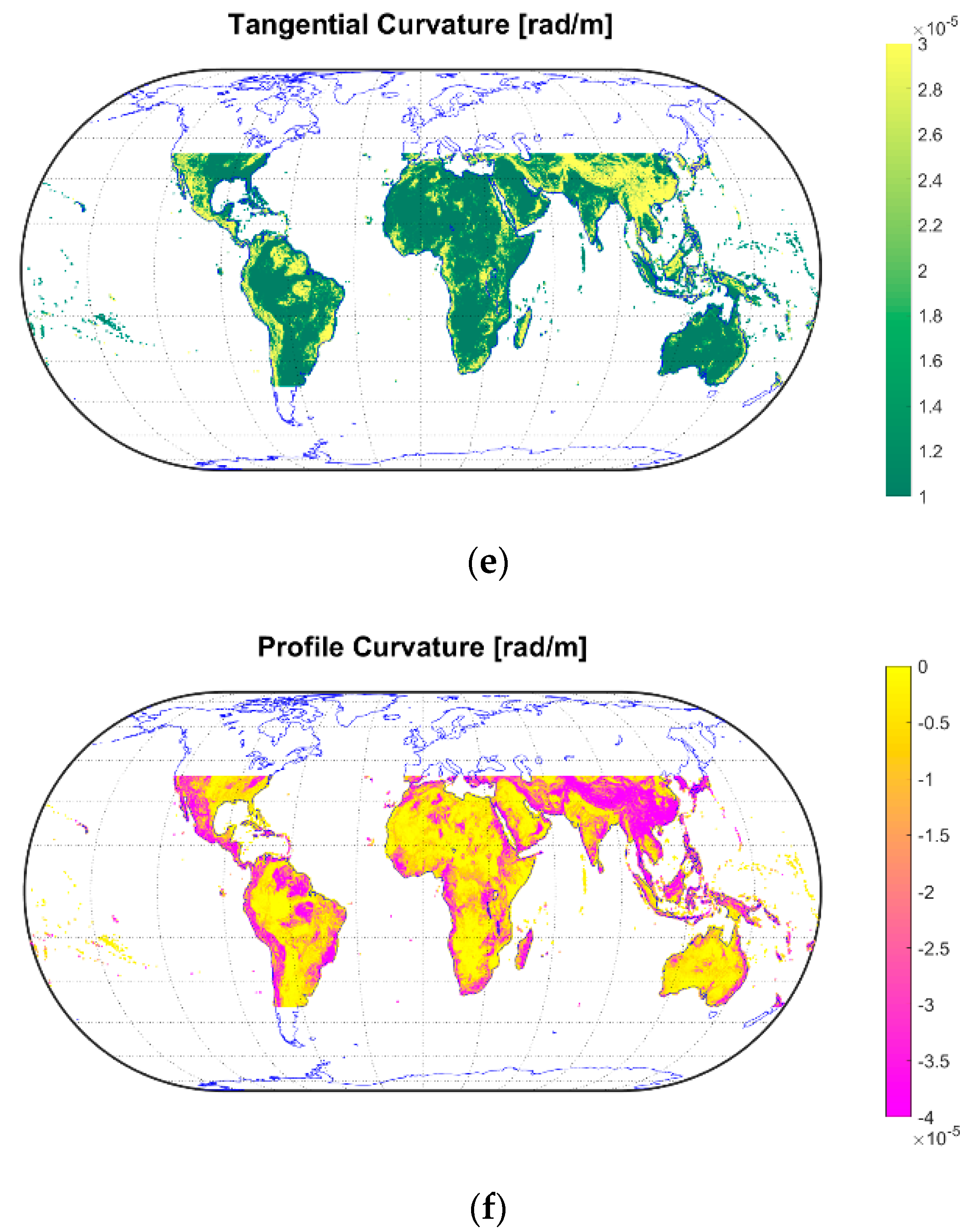
Overall, it was found that the spreading of was low ~ [100, 250] m and is high ~ [−10, −3] dB over flat areas with low topographic heterogeneity and small surface elevation gradients (Figure 2 and Figure 3). Over these areas, the scattering was quite specular and the coherence of the Earth-reflected GPS signals could be assumed to be high [35]. Under these circumstances,. Thus, the power of the reflected signals could be assumed to be roughly independent of the platform’s height (Equation.4). This point justifies the strong values of and the reduced spreading of the waveforms. SMC was high over regions that do not always correspond to flat areas (Figure 3d). On the other hand, the spatial patterns of & showed a certain agreement with . An exception is found over e.g., tropical rainforests. Here, the spreading of was high and was low because specular reflection is weakened by vegetation attenuation, , and vegetation structure contributes to diffuse scattering, both of which significantly modify the shape of [39]. A more quantitative analysis is performed at a regional scale over an area with little vegetation and low small-scale surface roughness. Over desert areas e.g., Sahara, Kalahari, and Australia it was found that was also quite high, despite SMC being almost negligible. This aspect was previously attributed to the effect of sub-surface scattering over rich sand content areas [6,9]. In very dry conditions, GNSS-R observables have shown a certain sensitivity to the soil moisture at deeper levels [8].
In addition, specular scattering over areas with high could significantly increase , despite SMC being low (Figure 3). Indeed, was rather low over areas with high , which is an additional indication of the specular nature of the scattering. accounted for saturation of SMC in local topographic converging areas and was used to predict zones of surface saturation and therefore organized spatial fields of SMC. It could be expected that inland water bodies, i.e., rivers, are predominant in regions with high , which could justify the specular nature of the scattering [29]. On the other hand, topographic heterogeneity (, , and ), , and curvature parameters (, ) are high over the Andes and Himalayan mountains, where is high because of the effect of diffuse scattering .
4.2. Regional Scale
4.2.1. Introduction
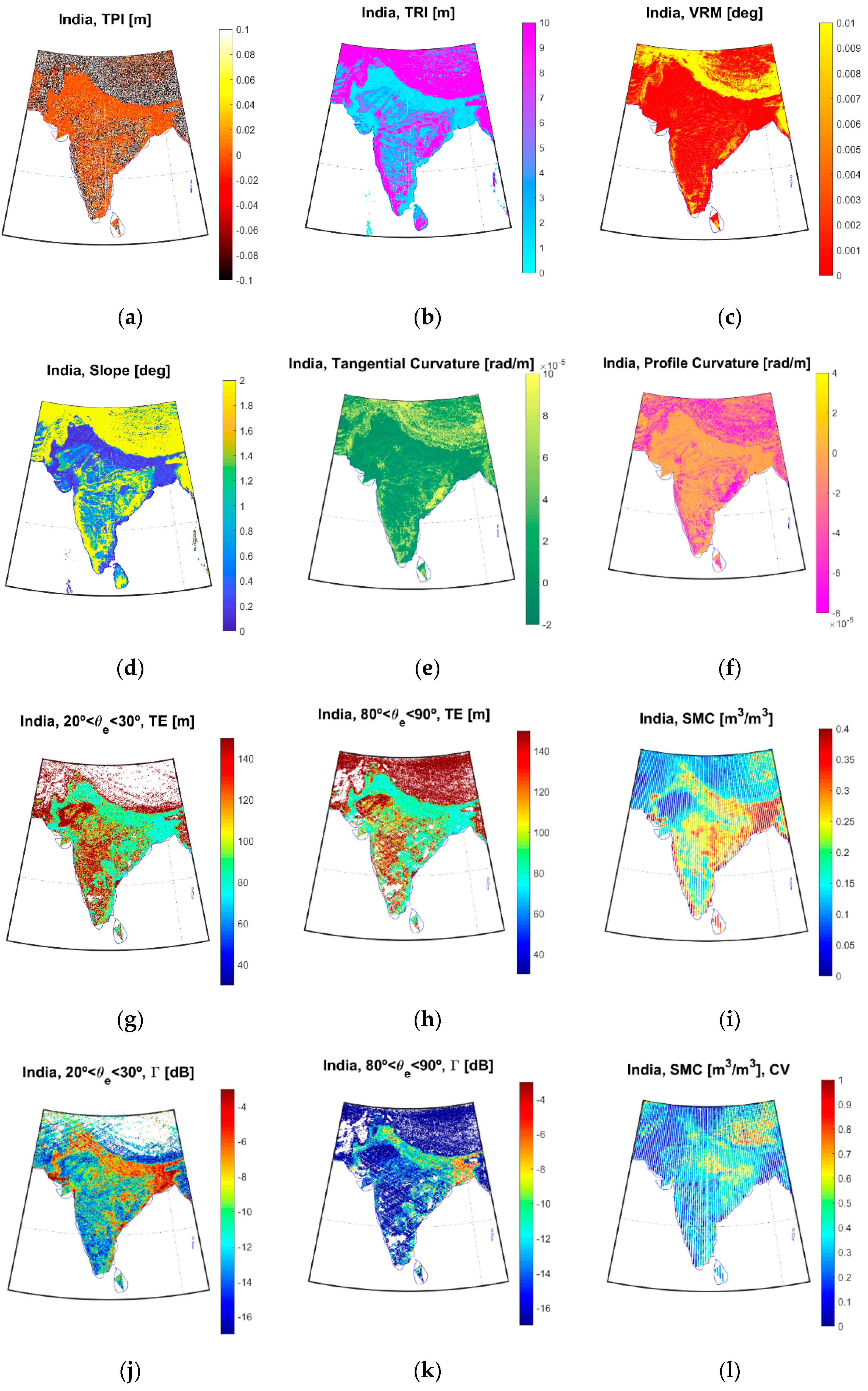
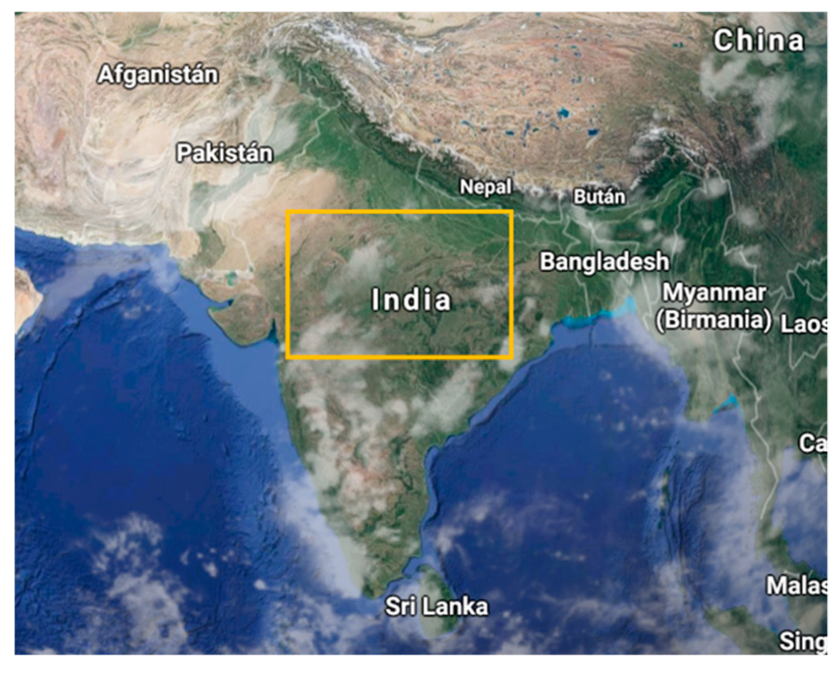
A specific target area over South Asia was selected to further investigate topographic effects in , without the influence of high levels of , above ground biomass (AGB), and canopy height (CH). The coordinates of the selected target area were as follows: latitude = [5, 36] ° and longitude = [64, 94] °. The characteristics of this region enabled this study to be performed over a rich variety of terrains, including the Tibetan Plateau, Great Himalaya, Indo-Gangetic Plains, and Hindustan. As such, the impact of different topographic features in and can be properly evaluated (Figure 4, Figure 5 and Figure 6). In so doing, were classified in two groups to evaluate the effects of topography over two different scenarios. At ~ [20, 30] °, the main contribution to the generation of the reflected signal in a specular manner (elevation angle of the incident wave equals elevation angle of the scattered wave i.e., = = ) came from surface facets over high elevation mountains. Some low elevation areas could be occulted by the top of the mountains. On the other hand, at ~ [80, 90] °, both valleys and mountain peaks could reflect signals in a specular manner towards the CyGNSS. This study was additionally complemented with SMAP-derived SMC and its coefficient of variation (CV). A wide range of SMC levels could be observed. The highest SMC values were associated with both the Indo-Gangetic Plains and mountains regions in the West of Hindustan, while the lowest SMC levels were found over the Tibetan Plateau and the Thar Desert. The spatial patterns of SMC did not appear correlated with the topographic parameters. Significant SMC levels could be found over mountains but also over rivers basins.
SMAP SMC data were used as an auxiliary product to help in the interpretation of the experimental results. The SMAP baseline accuracy requirement of 4% is not guaranteed over areas with very rough topography. SMC data are here provided with a lower accuracy. Nonetheless, 6 months of SMC data were averaged using a 0.1 ° x 0.1 ° latitude/longitude grid with a moving window of 0.2 ° in steps of 0.1 °. This strategy mitigated the effects of potential artefacts in SMAP-derived SMC. Additionally, this moving filter smoothed potential residual errors in the GMTED2010. Some errors have been reported over areas above Latitude ~ 60 ° [26]. However, this study was focused on areas within CyGNSS coverage Latitude ~ [−40, 40] °.
4.2.2. Interpretation of the Empirical Results
Figure 4 shows that increases and decreases with increasing values of the heterogeneity variables i.e., (Figure 4a), (Figure 4b), and (Figure 4c). Additionally, the measurements of (Figure 4d), (Figure 4e), and (Figure 4f) have a clear impact on both observables. The ranges of and are the same in all the plots. This strategy was assumed to provide intercomparable plots, and at the same time show full variability. Over the Himalayan mountains, the spreading of was very high (up to ~ 600 m) and was very low (down to ~ −25 dB). On the other hand, an inverse behavior appeared over the Indo-Gangetic Plains. Here, the scattered electromagnetic field became mostly coherent at grazing angles because the exponential factor (Equation (4)) increased significantly with decreasing angles [40]. As a consequence, there was an increment of , which was distributed in a rather homogeneous manner (Figure 4j), despite the strong SMC gradient from east to west (Figure 4i). In Reference [40] it was previously found that the dynamic range decreased at grazing angles. In other words, the sensitivity to SMC reduced at this geometry, which helps to justify the homogeneous distribution of . On the other hand, appeared more associated with the variability of SMC in a nadir-looking configuration, despite being lower than at grazing angles [8,40].
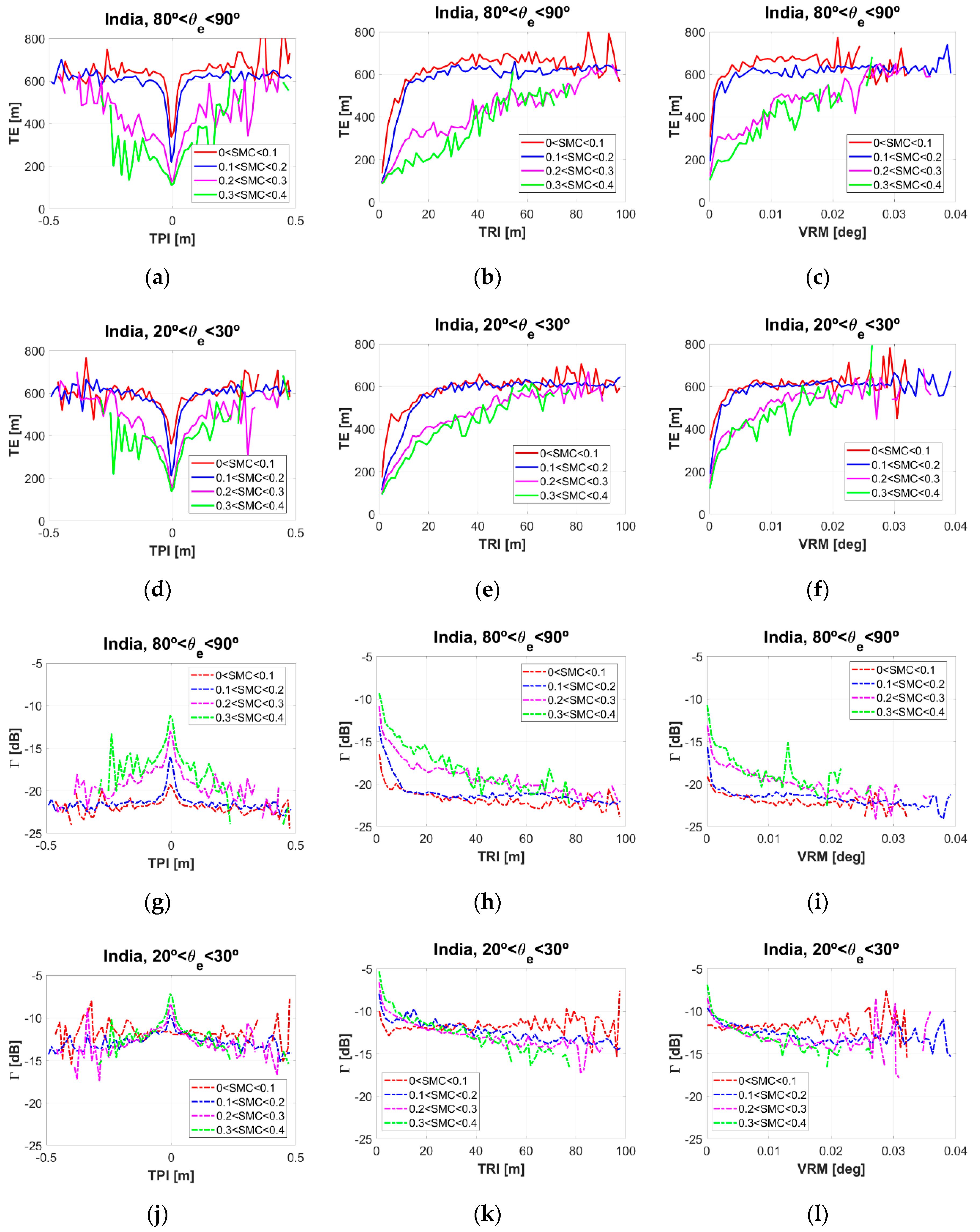
Figure 5 and Figure 6 show the relationship of and with the selected topographic parameters as a function of SMAP-derived SMC, over the two angular ranges used in this study ~ [20, 30] ° and ~ [80, 90] °: (Figure 5a,d,g,j), (Figure 5b,e,h,k), (Figure 5c,f,i,l), (Figure 6a,d,g,j), (Figure 6b,e,h,k), and (Figure 6c,f,i,l). The influence of SMC was evaluated at four differentiated ranges from ~0 m3/m3 to ~0.4 m3/m3 in steps of ~0.1 m3/m3.
For low SMC ~ [0, 0.2] m3/m3, the impact of the heterogeneity variables on both and was quite strong in the ranges ~ [−0.01, 0.01] m, ~ [0, 20] m, and ~ [0, 0.005] °. This point could be just justified because for low SMC levels: (a) the geometrical properties of the scattering medium play a stronger role than the dielectric properties and (b) the GNSS-R observables become saturated for a smaller topographic roughness.
Increasing SMC levels reduced the gradients because of the waveforms’ peak power increment. Consequently, the 70% power threshold appeared at smaller values as compared to dry soils. The variability of with SMC was higher in a nadir-looking configuration than at grazing angles because of the lower topographic influence. On the other hand, increased with increasing SMC in a nadir-looking configuration. However, it was roughly independent of SMC at grazing angles [8]. As such, the spreading of and the decrease of showed a much more gradual evolution for increasing heterogeneity levels up to ~ 600 m and ~ – 22 dB at ~ [80, 90] ° and ~ 600 m and ~ - 15 dB at ~ [20, 30] °.
Finally, it is pointed out that the topographic dynamic range of both GNSS-R parameters and was higher for SMC ~ [0, 0.2] m3/m3 than for SMC ~ [0.2, 0.4] m3/m3. This observation is also attributed to the stronger influence of the geometrical properties for decreasing SMC levels. A similar behavior was also pointed out in the case of the small-scale surface roughness [40].
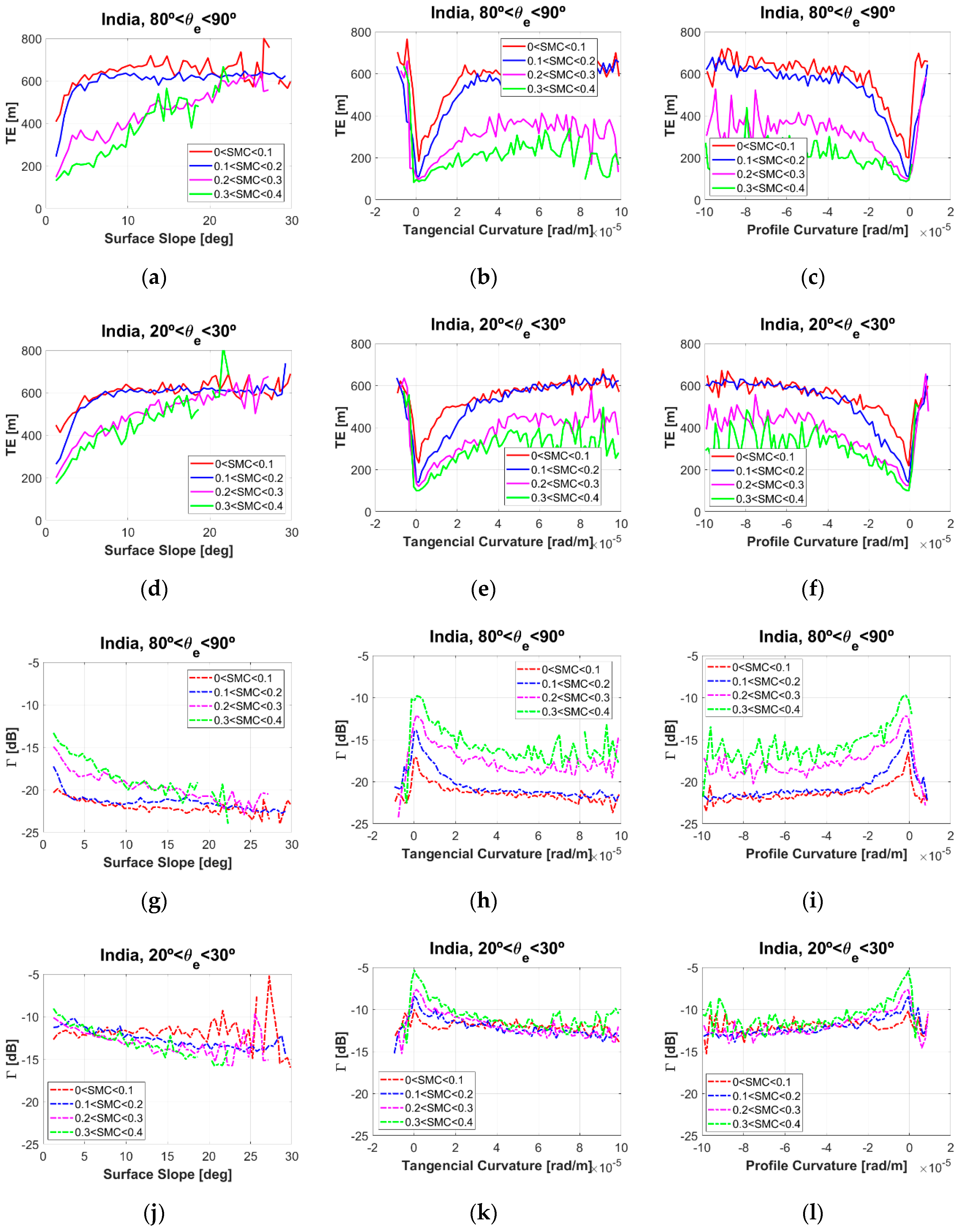
The impact of surface slopes and curvature variables on both observables, and , was quite strong at low SMC ~ [0, 0.2] m3/m3, over the following ranges: ~ [0, 5] °, ~ [-1, 2] rad/m, and ~ [−2, 1] rad/m. Increasing SMC levels reduced the gradients in agreement with the findings using the heterogeneity variables (Figure 5). The spreading of and the decrease of showed a much more gradual evolution for increasing curvature levels up to (a) ~ [20, 30] °: ~ 600 m and ~ – 13 dB for SMC ~ [0.3, 0.4] m3/m3, ~ 600 m and ~ – 13 dB for SMC ~ [0.2, 0.3] m3/m3, ~ 400 m and ~ – 13 dB for SMC ~ [0.1, 0.2] m3/m3, and ~ 300 m and ~ – 13 for SMC ~ [0, 0.1] m3/m3 and (b) ~ [80, 90] °: ~ 600 m and ~ – 16 dB for SMC ~ [0.3, 0.4] m3/m3, ~ 600 m and ~ – 18 dB for SMC ~ [0.2, 0.3] m3/m3, ~ 375 m and ~ – 22 dB for SMC ~ [0.1, 0.2] m3/m3, and ~ 200 m and ~ – 23 dB for SMC ~ [0, 0.1] m3/m3.
Surface slopes modify the scattering area with respect to that corresponding to a flat Earth assumption. They are a key parameter in GNSS-R studies over land surfaces, which have a certain degree of correlation with and because increasing topographic heterogeneity belongs to increasing surface slopes. On the other hand, the and have a much clearer differentiated impact on and . These topographic variables are directly related to water accumulation over the surface. Over flat surfaces, is high and is low because the curvature is negligible, and the scattering is quite specular. However, the impact of SMC is lower compared to areas with higher curvatures. In these areas, and have a clearer differentiated response to different SMC levels. Finally, it was found that the variability with SMC is higher in a nadir-looking configuration than at grazing angles. It increases for negative levels (concave), while for positive curvature levels (convex) there is a negligible of influence of SMC.
4.2.3. Sensitivity of CyGNSS to TWI vs. SMC
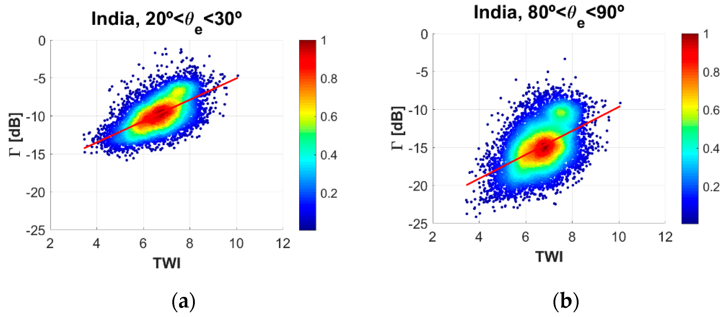
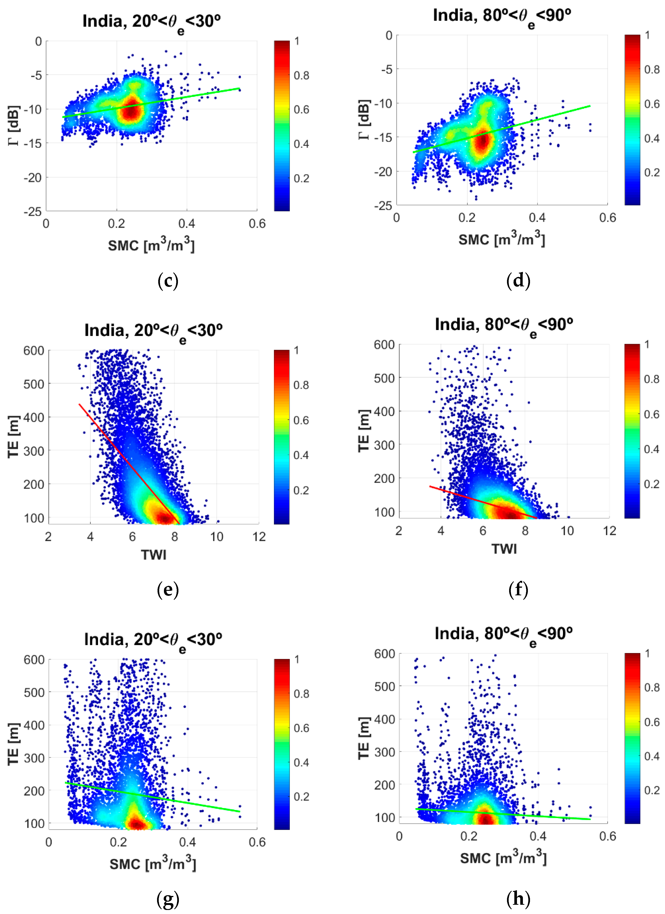
The strong influence of primary terrain attributes on GNSS-R observables (Figure 5 and Figure 6) triggered the sensitivity study of and with vs. SMC. To do so, a specific target area (Latitude ~ [20, 27] ° and Longitude ~ [72, 84] °) was selected with a strong gradient of SMC, and a wide topographic heterogeneity (Figure 7). Figure 8 shows the density scatter plots of vs. at ~ [20, 30] ° (Figure 8a) and ~ [80, 90] ° (Figure 8b), vs. SMC at ~ [20, 30] ° (Figure 8c) and ~ [80, 90] ° (Figure 8d), vs. at ~ [20, 30] ° (Figure 8e) and ~ [80, 90] ° (Figure 8f), and vs. SMC at ~ [20, 30] ° (Figure 8g) and ~ [80, 90] ° (Figure 8h).
Both observables and are more correlated with than with SMC (Table 1). This point could be justified because the potential presence of inland water bodies over areas with high have a stronger impact on GNSS-R observables than SMC. In this analysis, areas with high elevation and very rough topography (i.e., Himalayan mountains) were excluded (Figure 7) because SMAP-derived SMC could have some uncertainties over areas with very rough topography. As such, SMC is delivered within the baseline accuracy in this target area.
The Pearson correlation coefficients increased at grazing angles because of the stronger impact of topography at this geometry as compared to a nadir-looking configuration. On the other hand, the correlation of and with SMC is almost negligible despite the moderate-to-high SMC dynamic range ~ [0, 0.4] m3/m3. The slopes of the linear regressions were also included in Table 1, for both angular ranges. It is found that the sensitivity of to and SMC increased at grazing angles, while that of was stronger in a nadir-looking configuration in agreement with the results in Reference [8]. This empirical evidence suggests that topographic features can determine the main spatial pattern of Earth’s surface reflectivity, at least over some specific target areas.
Finally, it is worth pointing out that these results at a regional scale support qualitative results obtained at a global scale (Figure 1). As such, attention should be paid when analyzing GNSS-R data because soils saturated by the effect of topography could introduce confounding effects with respect to the impact of SMC.
5. Final Discussion
CyGNSS space-borne GNSS-R data appear to have a strong dependence on topography. This dependence was found to be different from that corresponding to small-scale surface roughness. The impact of topographic roughness increased with decreasing angles , while the impact of surface roughness increased with increasing . This latter point can be justified based on the Rayleigh criterion that establishes that a surface (without vegetation and rough topography) could be considered smooth if the phase difference between two reflected electromagnetic waves is lower than π/2 rad. On the other hand, it was found that topographic roughness was a much more complex phenomenon, which depended on several topographic features in a differentiated manner. Some Earth observation missions such as the Soil Moisture Ocean Salinity (SMOS) mission used a method to flag the pixels according to the relative impact of topography on the brightness temperature [41]. The GNSS-R scenario appears more complex because the bistatic scattering includes both a coherent and an incoherent component, in different proportions depending on the dielectric and geometrical properties of the scattering medium, and the directions of incoming and outgoing electromagnetic waves. On the other hand, the spatial resolution depends on the coherent-to-incoherent scattering ratio. This point complicates the topographic masking because of the impact of .
The scattering over surfaces with rough topography could be assumed to be totally incoherent. However, experimental results showed that increased with decreasing even over regions with very rough topography. This angular behavior is classically associated with the coherent scattering term because the effective surface roughness is much lower at grazing angles [40]. At this point, it could be hypothesized that the scattering could be locally coherent over specific mountains facets. The total scattered electromagnetic field could be coherent if only a single mountain facet contributes in a specular manner to the reflected signal as collected by CyGNSS.
6. Conclusions
Several topographic parameters, , , , , , and were derived from the ~250 m GMTED2010 DEM. The impact of these parameters on different GNSS-R observables and was assessed over land surfaces as a function of SMAP-derived SMC and . A parametric study was then performed over a target area in South Asia. For low SMC levels, and presented a strong fluctuation from flat surfaces to areas with moderate topographic roughness. On the other hand, increasing SMC levels reduced the gradients. Additionally, it was found that the sensitivity of both observables to SMC increased in a nadir-looking configuration as compared to grazing angles. As a final remark, and converged with increasing levels of , , , and ; while they diverge with increasing levels of and for different SMC values.
In the last part of this study, the sensitivity of and to and SMC was evaluated over a specific target region in North India, with a strong SMC gradient and a wide topography heterogeneity. Areas with very rough topography were excluded. The Pearson correlation coefficients of and with were rather high. On the other hand, the correlation with SMC was almost negligible. This empirical evidence suggests that topographic features could determine the main spatial patterns of , at least over some areas. provided an indication of the relative propensity of soils to become saturated to the surface due to the effect of the local topography.
Present and future applications of GNSS-R for Earth Observation over land surfaces could benefit from the results of this work. Accuracy on geophysical parameters retrieval e.g., SMC, could be improved after properly calibrated reflected DDMs. The estimation of SMC based on GNSS-R observables relies on their ability to represent the dielectric constant of the soil. However, topography significantly distorts these observables. The empirical relationships that were found between the selected topographic parameters and the observables pave the way to compensate underestimated SMC levels due to topographic roughness. Future work should include ground truth data to further validate these results.
Author Contributions
Conceptualization, methodology, software, investigation, and writing-original draft preparation by H.C.-L.; supervision, by G.L. and M.C.
Funding
This research received no external funding.
Acknowledgments
This research was carried out with the support grant of a Juan de la Cierva postdoctoral research fellowship from the Spanish Ministerio de Ciencia, Innovación y Universidades, reference FJCI-2016-29356.
Conflicts of Interest
The authors declare no conflict of interest.
References
- Dunne, T.; Black, R.D. Partial area contributions to storm runoff in a small New England watershed. Water Resour. Res. 1970, 6, 1296–1311. [Google Scholar] [CrossRef]
- Western, A.W.; Grayson, R.B.; Bloschl, G.G.; Willgoose, R.; McMahon, T.A. Observed spatial organization of soil moisture and its relation to terrain indices. Water Resour. Res. 1999, 35, 797–810. [Google Scholar] [CrossRef] [Green Version]
- Martín-Neira, M. A passive reflectometry and interferometry system (PARIS): Application to ocean altimetry. ESA J. 1993, 17, 331–355. [Google Scholar]
- Martín-Neira, M.; Li, W.; Andrés-Beivide, A.; Ballesteros-Sels, X. Cookie: A satellite concept for GNSS remote sensing constellations. IEEE J. Sel. Top. Appl. Earth Obs. Remote Sens. 2016, 9, 4593–4610. [Google Scholar] [CrossRef]
- Cardellach, E.; Rius, A.; Martín-Neira, M.; Fabra, F.; Nogués-Correig, O.; Ribó, S.; Kainulainen, J.; Camps, A.; D’Addio, S. Consolidating the precision of interferometric GNSS-R ocean altimetry using airborne experimental data. IEEE Trans. Geosci. Remote Sens. 2014, 52, 4992–5004. [Google Scholar] [CrossRef]
- Camps, A.; Hyuk, H.; Pablos, M.; Foti, G.; Gommerginger, C.P.; Liu, P.W.; Judge, J. Sensitivity of GNSS-R spaceborne observations to soil moisture and vegetation. IEEE J. Sel. Top. Appl. Earth Obs. Remote Sens. 2016, 9, 4730–4732. [Google Scholar] [CrossRef]
- Chew, C.; Shah, R.; Zuffada, C.; Hajj, G.; Masters, D.; Mannucci, A.J. Demonstrating soil moisture remote sensing with observations from the UK TechDemoSat-1 satellite mission. Geophys. Res. Lett. 2016, 43, 3317–3324. [Google Scholar] [CrossRef]
- Camps, A.; Vall·llossera, M.; Park, H.; Portal, G.; Rossato, L. Sensitivity of TDS-1 GNSS-R reflectivity to soil moisture: Global and regional differences and impact of different spatial scales. Remote Sens. 2018, 10, 1856. [Google Scholar] [CrossRef]
- Carreno-Luengo, H.; Lowe, S.T.; Zuffada, C.; Esterhuizen, S.; Oveisgharan, S. Spaceborne GNSS-R from the SMAP mission: First assessment of polarimetric scatterometry over land and cryosphere. Remote Sens. 2017, 9, 362. [Google Scholar] [CrossRef]
- Carreno-Luengo, H.; Luzi, G.; Crosetto, M. Sensitivity of CyGNSS bistatic reflectivity and SMAP microwave brightness temperature to geophysical parameters over land surfaces. IEEE J. Sel. Top. Appl. Earth Obs. Remote Sens. 2018, 12, 107–122. [Google Scholar] [CrossRef]
- Chew, C.; Small, E.E. Soil moisture sensing using spaceborne GNSS reflections: Comparison of CYGNSS reflectivity to SMAP soil moisture. Geophys. Res. Lett. 2018, 45, 4049–4057. [Google Scholar] [CrossRef]
- Ruf, C.; Cardellach, E.; Clarizia, M.P.; Galdi, C.; Gleason, S.T.; Paloscia, S. Foreword to the special issue on Cyclone Global Navigation Satellite System (CYGNSS) early on orbit performance. IEEE J. Sel. Top. Appl. Earth Obs. Remote Sens. 2018, 12, 1–4. [Google Scholar] [CrossRef]
- Park, H.; Camps, A.; Pascual, D.; Alonso-Arroyo, A.; Querol, J.; Onrubia, R. Improvement of PAU/PARIS end-to-end performance simulator (P2EPS): Land scattering including topography. In Proceedings of the IEEE International Geoscience and Remote Sensing Symposium, Beijing, China, 10–15 July 2016; pp. 5607–5610. [Google Scholar]
- Carreno-Luengo, H.; Luzi, G.; Crosetto, M. An experimental assessment of rough topography on spaceborne delay Doppler maps. In Proceedings of the IEEE GNSS+R Specialist Meeting on Reflectometry using GNSS and other Signals of Opportunity, Benevento, Italy, 20–22 May 2019; pp. 1–4. [Google Scholar]
- Ruf, C.; Atlas, R.; Chang, P.S.; Clarizia, M.P.; Garrison, J.L.; Gleason, S.; Katzberg, S.J.; Jelenak, Z.; Johnson, J.T.; Majumdar, S.J.; et al. New ocean winds satellite mission to probe hurricanes and tropical convection. Bull. Amer. Meteorol. Soc. 2015, 97, 385–395. [Google Scholar] [CrossRef]
- CYGNSS. CYGNSS Level 1 Science Data Record. Ver. 2.1. PO.DAAC, CA, USA. 2017. Available online: http://0-dx-doi-org.brum.beds.ac.uk/10.5067/CYGNSL1X20 (accessed on 11 May 2019).
- Zavorotny, V.U.; Voronovich, A.G. Scattering of GPS signals from the ocean with wind remote sensing applications. IEEE Trans. Geosci. Remote Sens. 2000, 38, 951–964. [Google Scholar] [CrossRef]
- Ulaby, F.T.; Long, D.G. Microwave Radar and Radiometric Remote Sensing; Univ. Michigan Press: Ann Arbor, MI, USA, 2014; p. 252. [Google Scholar]
- Pierdicca, N.; Guerriero, L.; Brogioni, M.; Egido, A. On the coherent and non-coherent components of bare soil and vegetated terrain bistatic scattering: Modelling the GNSS-R signal over land. In Proceedings of the IEEE International Geoscience and Remote Sensing Symposium, Munich, Germany, 22–27 July 2012; pp. 3407–3410. [Google Scholar]
- Carreno-Luengo, H.; Camps, A.; Querol, J.; Forte, G. First results of a GNSS-R experiment from a stratospheric balloon over boreal forests. IEEE Trans. Geosci. Remote Sens. 2015, 54, 2652–2663. [Google Scholar] [CrossRef]
- Voronovich, A.G.; Zavorotny, V.U. Bistatic radar equation for signals of opportunity revisited. IEEE Trans. Geosci. Remote Sens. 2017, 56, 1959–1968. [Google Scholar] [CrossRef]
- Tsang, L.; Newton, R.W. Microwave emissions from soils with rough surfaces. J. Geophys. Res. 1982, 87, 9017–9024. [Google Scholar] [CrossRef]
- Pierdicca, N.; Guerriero, L.; Giusto, R.; Brogioni, M.; Egido, A. SAVERS: A Simulator of GNSS Reflections from Bare and Vegetated Soils. IEEE Trans. Geosci. Remote Sens. 2014, 52, 6542–6554. [Google Scholar] [CrossRef]
- Zribi, M.; Guyon, D.; Motte, E.; Dayau, S.; Wigneron, J.-P.; Baghdadi, N.; Pierdicca, N. Performance of GNSS-R GLORI data for biomass estimation over the Landes forests. Int. J. Earth Obs. Geoinf. 2019, 74, 150–158. [Google Scholar] [CrossRef]
- Gleason, S. Reflecting on GPS sensing land and ice from low earth orbit. GPS World Innov. Column. 2007, 18, 44–49. [Google Scholar]
- Amatulli, G.; Domisch, S.; Tuanmu, M.-N.; Parmentire, B.; Ranipeta, A.; Malczyk, J.; Jetz, W. A suite of global cross-scale topographic variables for environmental and biodiversity modelling. Nat. Sci. Data 2018, 180040. [Google Scholar] [CrossRef] [PubMed]
- Wilson, M.F.J.; O’Connell, B.; Brown, C.; Guinan, J.C.; Grehan, A.J. Multiscale terrain analysis of multibeam bathymetry data for habitat mapping on the continental slope. Taylor Fr. Mar. Geod. 2007, 40, 3–35. [Google Scholar] [CrossRef]
- Wood, J. The Geomorphological Characterization of Digital Elevation Models. Ph.D. Thesis, University of Leicester, Leicester, UK, 1996. [Google Scholar]
- Beven, K.J.; Kirkby, M.J. A physically based, variable contributing area model of basin hydrology. Hydrol. Sci. Bull. 1979, 24, 43–69. [Google Scholar] [CrossRef]
- Wolock, D.M. Simulating the Variable-Source-Area Concept of Streamflow Generation with the Watershed Model TOPMODEL; United States Geological Survey Water-Resources Investigations Report 93-4124; US Geological Survey: Lawerence, KS, USA, 1993. [Google Scholar]
- Marthews, T.R.; Dadson, S.J.; Lehner, B.; Abele, S.; Gedney, N. High-resolution global topographic index values for use in large-scale hydrological modelling. EGU Hydrol. Earth Syst. Sci. 2015, 19, 91–104. [Google Scholar] [CrossRef] [Green Version]
- Lehner, B.; Grill, G. Global river hydrography and network routing: Baseline data and new approaches to study the world’s large river systems. Hydrol. Process. 2013, 27, 2171–2186. [Google Scholar] [CrossRef]
- Quinn, P.; Beven, K.; Chevalier, P.; Planchon, O. The prediction of hillslope flow paths for distributed hydrological modelling using digital terrain models. Hydrol. Process. 1991, 5, 59–79. [Google Scholar] [CrossRef]
- Quinn, P.; Beven, K.; Lamb, R. The ln (a/tanB) index: How to calculate it and how to use it within the TOPMODEL framework. Hydrol. Process. 1995, 9, 161–182. [Google Scholar] [CrossRef]
- Clarizia, M.-P.; Pierdicca, N.; Constantini, F.; Floury, N. Analysis of CyGNSS data for soil moisture retrieval. IEEE J. Sel. Top. Appl. Earth Obs. Remote Sens. 2019, 12, 2227–2235. [Google Scholar] [CrossRef]
- Al-Khaldi, M.; Johnson, J.T.; O’Brien, A.J.; Balenzano, A.; Mattia, F. Time-series retrieval of soil moisture using CYGNSS. IEEE Trans. Geosci. Remote Sens. 2019, 57, 4322–4331. [Google Scholar] [CrossRef]
- Entekhabi, D.; Yueh, S.; O’Neill, P.E.; Kellogg, K.H.; Allen, A.; Bindlish, R.; Brown, M.; Chan, S.; Colliander, A.; Crow, W.; et al. SMAP Handbook. Soil Moisture Active Passive. Available online: https://nsidc.org/data/ SPL3SMP_E/versions/1 (accessed on 6 April 2019).
- Chan, S.K.; Bindlish, R.; O’Neill, P.; Jackson, T.; Njoku, E.; Dunbar, S.; Chaubell, J.; Piepmeier, J.; Yueh, S.; Entekhab, D.; et al. Development and assessment of the SMAP enhanced passive soil moisture product. Remote Sens. Environ. 2018, 204, 931–941. [Google Scholar] [CrossRef]
- Carreno-Luengo, H.; Luzi, G.; Crosetto, M. Sensitivity of CyGNSS to above ground biomass and canopy height over tropical forests. In Proceedings of the IEEE GNSS+R Specialist Meeting on Reflectometry using GNSS and other Signals of Opportunity, Benevento, Italy, 20–22 May 2019; pp. 1–4. [Google Scholar]
- Carreno-Luengo, H.; Luzi, G.; Crosetto, M. Impact of the elevation angle on CyGNSS GNSS-R bistatic reflectivity as a function of effective surface roughness over land surfaces. Remote Sens. 2018, 10, 1749. [Google Scholar] [CrossRef]
- Mialon, A.; Coret, L.; Kerr, Y.H.; Secherre, F.; Wigneron, J.-P. Flagging the topographic impact on the SMOS signal. IEEE Trans. Geosci. Remote Sens. 2008, 46, 689–694. [Google Scholar] [CrossRef]
Figure 1.
Image of the raster grid. Numbering system is shown. is the value of the raster. Notation is simplified. is used for any × analysis window, where may be any odd integer smaller than the number of cells in the shortest side of the raster.
Figure 1.
Image of the raster grid. Numbering system is shown. is the value of the raster. Notation is simplified. is used for any × analysis window, where may be any odd integer smaller than the number of cells in the shortest side of the raster.

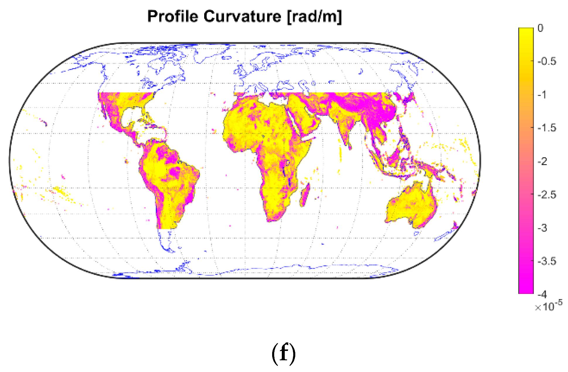
Figure 2.
Global Multi-resolution Terrain Elevation Data 2010 (GMTED2010) model-based topographic parameters. (a) Topographic position index () (m), (b) terrain ruggedness index () (m), (c) vector ruggedness measure () (deg), (d) Slope (deg), (e) tangential curvature () (rad/m), and (f) profile curvature () (rad/m). Parameters were displayed over the Cyclone Global Navigation Satellite System (CyGNSS) coverage over land surfaces.


Figure 3.
(a) , (b) CyGNSS-derived (dB), (c) CyGNSS-derived (m), and (d) Soil Moisture Active Passive (SMAP)-derived SMC (m3/m3). CyGNSS and SMAP data correspond to a temporal window of six months (1 August 2018 to 31 January 2019). The parameters were displayed over the CyGNSS coverage over land surfaces.

Figure 4.
Regional scale study over a target area in South Asia. Different scientific observables and auxiliary data were depicted: (a) , (b) , (c) , (d) , (e) , (f) , (g) CyGNSS-derived at ~ [20, 30] °, (h) at ~ [80, 90] °, (i) SMAP-derived SMC, (j) CyGNSS-derived at ~ [20, 30] °, (k) at ~ [80, 90] °, and (l) SMC CV.

Figure 5.
Parametric evaluation as a function of SMAP-derived SMC: (a,d,g,j) , (b,e,h,k) , and (c,f,i,l) . Analysis of CyGNSS-derived at ~ [80, 90] ° (a–c) and ~ [20, 30] ° (d–f). Analysis of CyGNSS-derived at ~ [80, 90] ° (g–i) and ~ [20, 30] ° (j–l).
Figure 5.
Parametric evaluation as a function of SMAP-derived SMC: (a,d,g,j) , (b,e,h,k) , and (c,f,i,l) . Analysis of CyGNSS-derived at ~ [80, 90] ° (a–c) and ~ [20, 30] ° (d–f). Analysis of CyGNSS-derived at ~ [80, 90] ° (g–i) and ~ [20, 30] ° (j–l).

Figure 6.
Parametric evaluation as a function of SMAP-derived SMC: (a,d,g,j) , (b,e,h,k) , and (c,f,i,l) . Analysis of CyGNSS-derived at ~ [80, 90] ° (a–c) and ~ [20, 30] ° (d–f). Analysis of CyGNSS-derived at ~ [80, 90] ° (g–i) and ~ [20, 30] ° (j–l).
Figure 6.
Parametric evaluation as a function of SMAP-derived SMC: (a,d,g,j) , (b,e,h,k) , and (c,f,i,l) . Analysis of CyGNSS-derived at ~ [80, 90] ° (a–c) and ~ [20, 30] ° (d–f). Analysis of CyGNSS-derived at ~ [80, 90] ° (g–i) and ~ [20, 30] ° (j–l).

Figure 7.
Close up of the area selected for the sensitivity analysis of CyGNSS observables to and SMAP-derived SMC.
Figure 7.
Close up of the area selected for the sensitivity analysis of CyGNSS observables to and SMAP-derived SMC.

Figure 8.
Density scatter plots over North India target area: CyGNSS-derived vs. at (a) ~ [20, 30] ° and (b) ~ [80, 90] °. vs. SMAP-derived SMC at (c) ~ [20, 30] ° and (d) ~ [80, 90] °. vs. at (e) ~ [20, 30] ° and (f) ~ [80, 90] °. vs. SMC at (g) ~ [20, 30] ° and (h) ~ [80, 90] °.
Figure 8.
Density scatter plots over North India target area: CyGNSS-derived vs. at (a) ~ [20, 30] ° and (b) ~ [80, 90] °. vs. SMAP-derived SMC at (c) ~ [20, 30] ° and (d) ~ [80, 90] °. vs. at (e) ~ [20, 30] ° and (f) ~ [80, 90] °. vs. SMC at (g) ~ [20, 30] ° and (h) ~ [80, 90] °.


Table 1.
Statistics (Pearson correlation coefficient , RMSE, and slope of the linear fits) of the scatter plots of CyGNSS-derived and with and SMAP-derived SMC over the selected target area over North India.
Table 1.
Statistics (Pearson correlation coefficient , RMSE, and slope of the linear fits) of the scatter plots of CyGNSS-derived and with and SMAP-derived SMC over the selected target area over North India.
| SMC [m3/m3] | ||||||||
|---|---|---|---|---|---|---|---|---|
| [m] | [dB] | [m] | [dB] | [m] | [dB] | [m] | [dB] | |
| [20, 30] ° | [20, 30] ° | [80, 90] ° | [80, 90] ° | [20, 30] ° | [20, 30] ° | [80, 90] ° | [80, 90] ° | |
| −0.63 | 0.59 | −0.50 | 0.48 | −0.08 | 0.27 | −0.06 | 0.30 | |
| RMSE | 95.3 | 1.7 | 68.5 | 2.7 | 121.9 | 2.1 | 80.7 | 2.8 |
| Slope | −75.13 | 1.40 | −18.65 | 1.57 | −175.21 | 8.4078 | −63.47 | 13.55 |
© 2019 by the authors. Licensee MDPI, Basel, Switzerland. This article is an open access article distributed under the terms and conditions of the Creative Commons Attribution (CC BY) license (http://creativecommons.org/licenses/by/4.0/).
Share and Cite
MDPI and ACS Style
Carreno-Luengo, H.; Luzi, G.; Crosetto, M. First Evaluation of Topography on GNSS-R: An Empirical Study Based on a Digital Elevation Model. Remote Sens. 2019, 11, 2556. https://0-doi-org.brum.beds.ac.uk/10.3390/rs11212556
AMA Style
Carreno-Luengo H, Luzi G, Crosetto M. First Evaluation of Topography on GNSS-R: An Empirical Study Based on a Digital Elevation Model. Remote Sensing. 2019; 11(21):2556. https://0-doi-org.brum.beds.ac.uk/10.3390/rs11212556
Chicago/Turabian StyleCarreno-Luengo, Hugo, Guido Luzi, and Michele Crosetto. 2019. "First Evaluation of Topography on GNSS-R: An Empirical Study Based on a Digital Elevation Model" Remote Sensing 11, no. 21: 2556. https://0-doi-org.brum.beds.ac.uk/10.3390/rs11212556
Note that from the first issue of 2016, this journal uses article numbers instead of page numbers. See further details here.