Evaluation and Application of Multi-Source Satellite Rainfall Product CHIRPS to Assess Spatio-Temporal Rainfall Variability on Data-Sparse Western Margins of Ethiopian Highlands

Abstract

The spatio-temporal characteristic of rainfall in the Beles Basin of Ethiopia is poorly understood, mainly due to lack of data. With recent advances in remote sensing, satellite derived rainfall products have become alternative sources of rainfall data for such poorly gauged areas. The objectives of this study were: (i) to evaluate a multi-source rainfall product (Climate Hazards Group Infrared Precipitation with Stations: CHIRPS) for the Beles Basin using gauge measurements and (ii) to assess the spatial and temporal variability of rainfall across the basin using validated CHIRPS data for the period 1981–2017. Categorical and continuous validation statistics were used to evaluate the performance, and time-space variability of rainfall was analyzed using GIS operations and statistical methods. Results showed a slight overestimation of rainfall occurrence by CHIRPS for the lowland region and underestimation for the highland region. CHIRPS underestimated the proportion of light daily rainfall events and overestimated the proportion of high intensity daily rainfall events. CHIRPS rainfall amount estimates were better in highland regions than in lowland regions, and became more accurate as the duration of the integration time increases from days to months. The annual spatio-temporal analysis result using CHIRPS revealed: a mean annual rainfall of the basin is 1490 mm (1050–2090 mm), a 50 mm increase of mean annual rainfall per 100 m elevation rise, periodical and persistent drought occurrence every 8 to 10 years, a significant increasing trend of rainfall (~5 mm year⁻¹), high rainfall variability observed at the lowland and drier parts of the basin and high coefficient of variation of monthly rainfall in March and April (revealing occurrence of bimodal rainfall characteristics). This study shows that the performance of CHIRPS product can vary spatially within a small basin level, and CHIRPS can help for better decision making in poorly gauged areas by giving an option to understand the space-time variability of rainfall characteristics.

1. Introduction

Developing countries, including Ethiopia with rapid population growth, depend on rainfed agriculture, which is highly vulnerable to fluctuations in rainfall amount. Information about rainfall plays a big role in several applications: for water resource development like agriculture and hydro-power generation [1,2,3,4], for monitoring ecological systems, flood, drought and disaster management [5,6,7]. Evaluation of spatio-temporal variability of rainfall demands reliable and spatially well distributed long-term observational records. However, in developing countries, observations of rainfall measurements from traditional ground weather stations are characterized by sparse, uneven distribution, poor data quality, temporally inconsistent and unable to access the data in time [8,9,10]. Those problems are more common in inaccessible and rugged areas [11] such as the highlands of Ethiopia, where rainfall is extremely variable over short distances [12,13]. The location of ground stations do not followed any particular criteria, except for being located in towns along main roads [8,14]. Because of this sparse distribution of gauging stations, estimating the spatial distribution of rainfall over remote parts of Ethiopia remains difficult. Therefore, evaluation of spatio-temporal variability of rainfall solely based on station data is a challenging task in most developing countries such as Ethiopia [2,15]. Furthermore, analysis using point-based rain gauge observations is limited to the given particular location, which provides a poor estimation of spatial distribution of rainfall for areas such as Ethiopia, where rainfall is extremely variable over short distances. To overcome these limitations, the recently developed long-term and spatially distributed satellite-based rainfall estimates have become important sources of rainfall data to analyze the spatial and temporal variability of rainfall, especially for data-sparse regions [8,16,17].

Satellite derived rainfall estimates (SREs) provide synoptic data at different temporal and spatial scales, and play a key role for hydrological applications [18,19]. SREs could, therefore, be a solution to overcome the lack of rainfall data over remote and inaccessible areas [8,20], such as the Beles Basin of Ethiopia. SREs provide historical records of spatially distributed rainfall estimates where rain gauge stations are poorly (or not) distributed. At present, several high-resolution satellite rainfall products are available free of charge with varying design objective, data sources, spatial coverage, spatial and temporal resolution [7,8,14].

Thermal infrared (TIR) and passive microwave (PMW) sensors (from geostationary and low-Earth-orbiting satellites respectively) or combinations of both are commonly used in SREs algorithms to retrieve rainfall data from satellite [21,22,23]. SREs provide indirect estimates of rainfall by measuring cloud thickness (PMW) or cloud top temperature (TIR). Each approach has limitations. TIR-based rainfall estimates have limitations in detecting local variations in rainfall, effect of warm rain processes and possible misinterpretation of cirrus clouds as rain clouds [21,23,24]. The limitations of PMW-based SREs are the identification of warm and orographic rains, background emission from the land surface, low repetition rate and coarser spatial resolutions [22,23]. Recently, combining PMW (the better rainfall identification) with TIR images (the higher spatial and temporal frequency) and further blending gauge measurements is producing better satellite rainfall products [25].

It is important to realize that satellites measure rainfall indirectly which induces uncertainties attributed with retrieval algorithms, sampling frequency and satellite instrument sensors themselves [8,17,22]. Therefore, validation of satellite rainfall products is necessary at varying spatial and temporal scales before integration into operational applications such as rainfall pattern and variability study [14,16]. Recently, rigorous validation of different satellite products has been performed to assure the quality in using the satellite products for different applications. The validations are done by comparing to gauge measurements. Each validation found different performance at different geographical regions, topographic conditions and seasons [2,7,9,11,14,15,16,17,18,19,20,23,26,27,28,29,30,31]. Comparisons between different satellite rainfall products have been done mainly at regional scale. Often substantial differences in performance were found. Evaluation and comparison of many satellite rainfall products have been conducted in East Africa [8,14,16,20,32] and other parts of the tropics [26,27,33]. The results show that the Climate Hazards Group InfraRed Precipitation with Stations (CHIRPS) product (a new multi-source precipitation climatology database, which has relatively high spatial resolution and long-term time series) performs better than most long-term satellite rainfall products.

Recently, evaluation of multi-source CHIRPS rainfall products and some spatio-temporal analyses of rainfall using CHIRPS over Eastern-Africa regions [8,16,30,33,34,35,36] indicates a potential to be used for various applications like rainfall pattern and variability study, including for the Upper Blue Nile basin of Ethiopian. Nevertheless, site-specific local validation of SREs at diverse physiographic settings has been recommended before using it for any operational applications [8,16,26,37].

In the past four decades, a number of changes have happened in the less accessible fertile bush-savanna lowland environment of the Beles Basin, which includes resettlements from highland regions in the early 1980s after severe famine [38,39] and huge water transfers from Lake Tana via a 12-km-long tunnel for the Tana-Beles hydroelectric project (since May 2010), rather than following the Blue Nile gorge [40,41]. As a result, there has been a change in socio-economic dynamics, deforestation, land degradation and conflicts for land and water [39,42]. This basin is considered as one of the growth corridors of Ethiopia. Despite the unavailability of climatic data (mainly rainfall) that hinders a detailed study of the hydrology of the area, large-scale development projects such as the Grand Ethiopian Renaissance Dam (GERD), sugar factories and a number of commercial farms have been started. Understanding rainfall patterns and possible trends as a function of space and time is crucial to help formulate mitigation measures and evaluate ecosystem resilience towards such variability [43]. Therefore, the main objectives of this study are: (i) to evaluate the newly available CHIRPS rain-fall product for the Beles Basin, (ii) to characterize the spatial and temporal variability of rainfall (after validation) within the Beles Basin, where distributed gauge meteorological data are very scarce.

2. Study Area and Data Sets

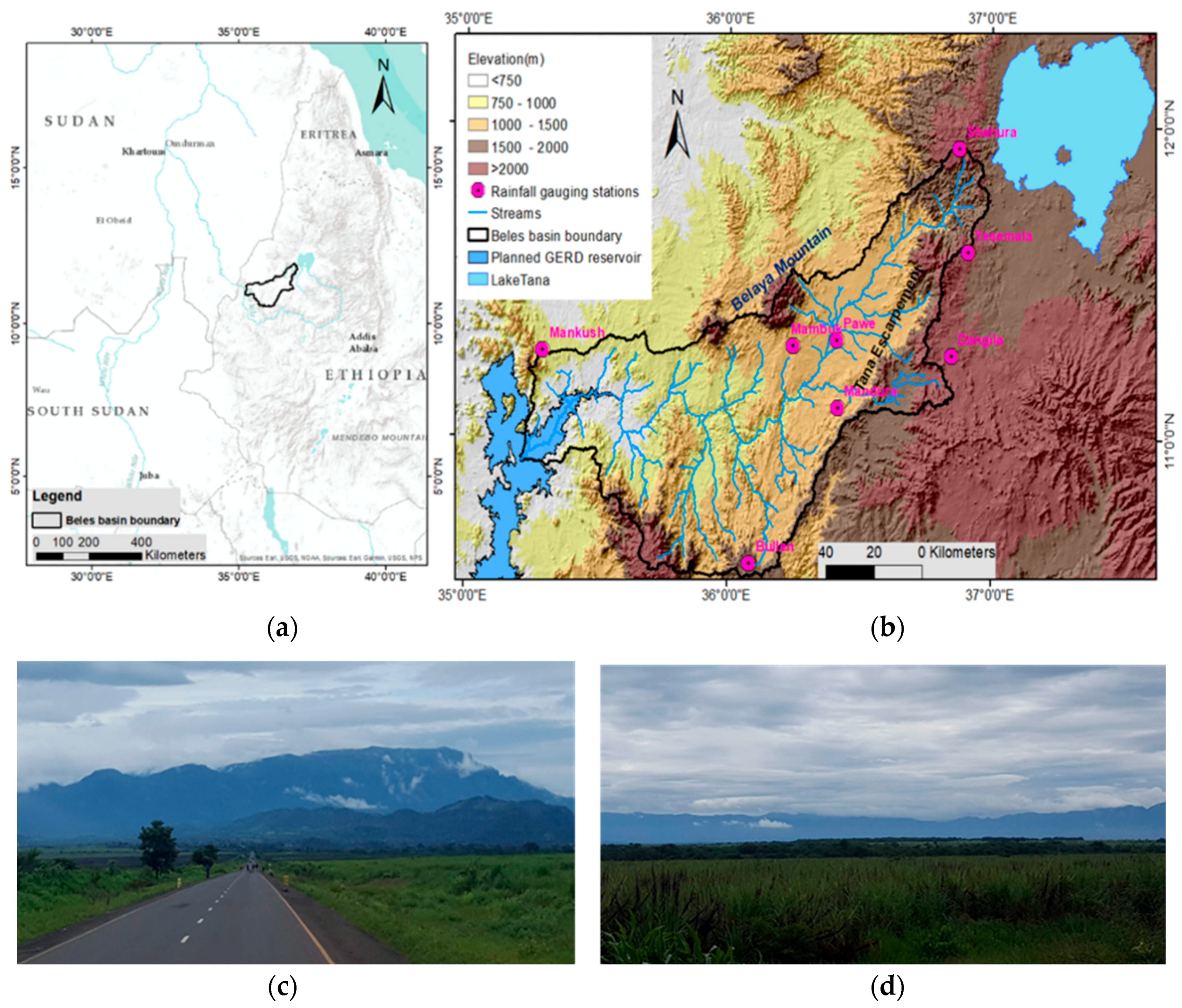
2.1. Study Area

The Beles Basin is one of the major sub-basins of the Upper Blue Nile Basin, which represents 8% of the total area of the basin. Beles River originates from the escarpment of south-western of Lake Tana, flows towards southwest, and joins the Blue Nile River just before it crosses the Ethio–Sudanese border (Figure 1). The nature of rainfall in the study area is unimodal and ~70–80% of the total rainfall is received between June and September [44], with annual yearly rainfall totals of about 1490 mm. The highly varied topography of the Beles Basin (577 m to 2735 m), together with the highly variable rainfall and temperature, results in contrasting climatic zones within the basin [45].

Meteorological data from gauging stations located inside within and close to the study basin do not have a long-term continuous recorded data (most of them become operational since 2005). Moreover, the data records are not consistent and the gauging stations are not spatially well distributed across the basin. It is one of poorly climatic gauged basins in Ethiopia. Topographically, available gauging stations can be divided into two groups; lowlands (elevations < 1500 m) and highlands (elevations > 1500 m) in line with contrasts in average monthly rainfall during the period of 2005–2015 (Figure 2).

2.2. Data Sets

2.2.1. Gauge Rainfall Data

Data from eight ground-based rain gauge stations, four from lowland areas (Mandura, Pawie, Manbuk and Mankush stations) and four from highland areas (Bullen, Dangela, Yesemala and Shahura stations) (Figure 1), were used as a reference to evaluate the accuracy of the CHIRPS rainfall product in Beles Basin. The nearby Dangela station has been considered for this analysis to be a highland gauge station, even though it is located out of the study area, to ensure that the analysis included four gauge stations for each region. All rain gauge stations used for evaluation are independent stations and they were not used in the creation of the CHIRPS data. The data source of these ground rain gauge stations were from the Ethiopian National Meteorological Agency (NMA) (http://www.ethiomet.gov.et/). Most stations have relatively better continuous data with little or no missing data for this period. In addition to the routine activity of quality checks by the NMA, extensive evaluations were performed on the entire data set to determine data completeness and quality.

2.2.2. CHIRPS Data

Climate Hazards Group Infrared Precipitation with Station data (CHIRPS) is a multi-source product database developed by U.S. Geological Survey (USGS) and University of California, Santa Barbara (UCSB) [25]. CHIRPS incorporates quasi-global geostationary thermal infrared satellite observations, Tropical Rainfall Measuring Mission’s (TRMM) 3B42 product, monthly precipitation climatology CHPClim (Climate Hazards Group Precipitation Climatology), atmospheric model rainfall fields from NOAA CFS (Climate Forecast System) and blending with precipitation observations from various sources, including national or regional Meteorological Services. From 1981 to present, CHIRPS incorporates 0.05° resolution gridded rainfall time series with daily temporal scale and quasi-global coverage.

The CHIRPS algorithm involves two part process [25]. First, using local regressions between Tropical Rainfall Measuring Mission multi-satellite precipitation analysis pentads and cold cloud duration (CCD) (<235 K), Infrared Precipitation pentad rainfall estimates are created. This created value converted into millimeters of precipitation by using local regression with TRMM 3B42 precipitation pentads. Then, in order to produce an unbiased gridded estimate the temporal component of IRP pentadal is multiplied by the spatial component CHPClim pentadl and produces the Climate Hazards Group IR Precipitation (CHIRP). The second step is blending CHIRP data with ground stations gauge data to produce the final product CHIRPS. The precipitation of a given pixel and the nearby stations are used to combine CHIRP with station observations at the pentadal and monthly time scales (most of the available data are at monthly time scale). Daily CHIRPS values are also created for Africa using daily cold cloud duration percentages (%CCD) by disaggregating the pentadal estimates (the corresponding pentadal rainfall is partitioned among the daily rain events proportional to their %CCD). In this study, we used the CHIRPS version 2.0 dataset (ftp://chg-ftpout.geog.ucsb.edu/pub/org/chg/products/CHIRPS-2.0/) of daily, monthly and yearly precipitation data from 2005 to 2015 for validation, and from 1981 to 2017 for spatio-temporal analysis of rainfall variability within the Beles Basin.

3. Methodology

3.1. Validation Techniques

The main focus of this validation work was to evaluate the performance of the CHIRPS over the Beles Basin before it was used for spatial and temporal analysis of rainfall variability within the basin. The evaluation was done both at daily and monthly time scale levels at which most of the hydrological analyses are performed. The validation was done by comparing CHIRPS rainfall products with ground-based observations for a time period of 2005 to 2015, during which good quality gauged data are available for the Beles Basin from Ethiopian Meteorological Agency. In areas where observation stations are scarcely distributed, such as in the Beles Basin, interpolating the ground-based gauge measurements to a gridded dataset is not advisable (because of large uncertainties). Therefore, the evaluation was performed based on a point to pixel analysis, disregarding the locations of the stations within the pixel. Consequently, random errors were expected to be introduced. This is because of uncertainties in rain gauge measurements and differences in the location of the reference gauges and pixel centers [8,46,47]. The evaluation was done for the lowland and highland regions separately considering that different characteristics of rainfall could show different performances of CHIRPS rainfall estimates [8,21]. We note that there is missing data at gauging stations especially at stations of lowland regions. The missing daily data values of gauge measurements were excluded from the analysis. The validation statistics that were used include the categorical statistics to assess the skill of CHIRPS in detecting the rainfall occurrence at daily time-scale and the continuous validation statistics on assessing rainfall totals, which are discussed below.

3.1.1. Categorical Validation Statistics (Rainfall Detection Capabilities)

To assess CHIRPS rain-detection capabilities, basic categorical validation statistics were used. The categorical validation statistics used were derived from a contingency table involving four event combinations of binary skill scores: (1) hits (A), when both rain gauge and CHIRPS detect precipitation, (2) false alarms (B), when CHIRPS failed to detect the no-rain case, (3) misses (C), when the CHIRPS failed to detect rain and (4) correct negatives (D), when both rain gauge and CHIRPS detect no precipitation (

Table 1. Contingency table for comparing CHIRPS satellite-based rainfall estimates and rain gauge observations (daily rainfall threshold used is 1 mm). The four possibilities are true positive (A), false positive (B), false negative (C) and true negative (D).

	CHIRPS ≥ 1 mm	CHIRPS < 1 mm
Gauge ≥ 1 mm	A	C
Gauge < 1 mm	B	D

). A rainfall threshold ≥1 mm was used to determine rain or no rain event. The 1 mm daily rainfall is the smallest nonzero recorded value at gauging stations and the 1 mm threshold has also been used in previous similar studies in region [8].

Categorical validation statistics [48] is widely used for the evaluation of the skill of the satellite at a daily time-scale in detecting the occurrence of rainfall [8,11,14,17,20,28]. The validation statistics used are the probability of detection (POD), false alarm ratio (FAR), Frequency bias index (FBI) and the Heidke Skill Score (HSS) (

Table 2. Statistical formulas to rainfall detection capabilities of CHIRPS based on categorical metrics, where: A, B, C and D represent hits, false alarms, misses and correct negatives, respectively (Table 1).

Statistic	Equation	Range	Best Value
Probability of detection (POD)	$POD=\frac{A}{A+C}$	0 to 1	1
False alarm ratio (FAR)	$FAR=\frac{B}{A+B}$	0 to 1	0
Frequency bias index (FBI)	$FBI=\frac{A+B}{A+C}$	0 to ∞	1
Heidke skill score (HSS)	$HSS=\frac{2\left(AD-BC\right)}{\left(A+C\right)\left(C+D\right)+\left(A+B\right)\left(B+D\right)}$	−∞ to 1	1

). The POD measures the skill of the satellite product in detecting the occurrence of rainfall; this ranges from 0 to a perfect score of 1. FAR assesses false detections ranging from 0 to 1 with a perfect score of 0. FBI compares the rainfall day detection frequency of the satellite product with that of the gauge measurements; it ranges from 0 to infinity with a perfect score of 1; FBI of less than 1 indicates an underestimation whereas FBI greater than 1 indicates an overestimation of rainfall days by CHIRPS. The HSS statistic measures the accuracy of the estimates, while accounting for matches due to random chances (after rain events detected by random chance have been removed), ranges from minus infinity to 1, HSS < 0 indicates that random chance is better than the satellite product, HSS = 0 means the product has no skill and HSS = 1 indicates a perfect estimation of precipitation by the satellite estimate product.

3.1.2. Continuous Validation Statistics (Assessment of Rainfall Totals)

To evaluate CHIRPS rainfall product performance in estimating the amount of the rainfall, we used four commonly used comparison (error) statistics indicator metrics: mean error (ME), mean absolute error (MAE), the Nash-Sutcliffe efficiency coefficient (NSE) and Bias (

Table 3. Statistical measures of performance, used for analysis based on continuous metrics, where: G = the rainfall total at a reference gauging station, $\overline{G}$ = the mean observed rainfall total at a reference gauging station, S = rainfall total for a satellite product, and N = the number of data pairs compared.

Statistic	Equation	Range	Best Value	Unit
Mean error (ME)	$ME=\frac{1}{N}\sum \left(S-G\right)$	−∞ to +∞	0	mm
Mean absolute error (MAE)	$MAE=\frac{1}{N}\sum \mid \left(S-G\right)\mid$	0 to +∞	0	mm
Nash-Sutcliffe efficiency coefficient (NSE)	$NSE=1-\frac{\sum {\left(G-S\right)}^2}{\sum {\left(G-\overline{G}\right)}^2}$	−∞ to 1	1
Bias	$Bias=\frac{\sum S}{\sum G}$	0 to +∞	1

), at daily and monthly time frames. Correlation coefficients were not used in the assessment because it is oversensitive to extreme values (outliers) and insensitive to additive and proportional differences [49] between satellite products and gauge measurements, especially at daily estimations.

ME and MAE have dimensions in mm, whereas NSE and Bias are dimensionless. ME (ranges from −∞ to ∞) and MAE (ranges from 0 to ∞) both provide information on the average magnitude of the estimation error and the perfect score for both is 0. Here, the widely used root mean squared error (RMSE) is replaced by the MAE to avoid the effect of extremely high rainfall values or outliers [49]. The NSE explains the relative magnitude of the variance of the residuals compared to the variance of the observed values of precipitation [50]; it ranges from −∞ to 1, where higher values mean that there is a better agreement between the satellite estimates and gauge measurements, while negative values indicate that the reference mean is a better estimate than the satellite estimates and 0 indicates that the reference mean is as good as the satellite rainfall estimates. The Bias ranges from 0 to ∞ and it shows how good the estimated mean and gauge mean correspond, with 1 being a perfect score. Combination of values of Bias >1 and positive ME values indicate an overestimation, whereas values of Bias <1 and negative ME indicate an underestimation [8]. Additional to these four commonly used comparison statistics metrics, the cumulative distribution function (CDF) for the proportion of rainfall events at daily scale, and scatter plot at monthly time scale were used to evaluate rainfall totals.

3.2. Assessment of Spatio-Temporal Variability and Trends of Rainfall

After the validation of CHIRPS product at the Beles Basin, annual and monthly CHIRPS rainfall product was used to assess the spatial and temporal variability of rainfall within the basin for a time series of 37 years (1981–2017). The analysis was done in a GIS environment and R statistics. We have examined the temporal and spatial rainfall variability and trends in the basin.

3.2.1. Assessment of Spatial Variability of Rainfall

Long term mean annual and monthly CHIRPS rainfall maps were calculated to visualize regional spatial and temporal patterns using cell (grid) statistics. Rainfall distribution is affected by topography and local climate [51], especially in topographically complex regions such as the Beles Basin. To evaluate the spatial patterns of rainfall with topography, long term mean annual rainfall was compared and evaluated with elevation across the basin area with two transect lines (East-West and Northeast-Southwest direction). The two transect lines were selected in the way to show variability of rainfall, from the lowland areas in the South-West of the basin to the Eastern and West to Northeastern Highlands, to assess the rainfall variability/trend over various topographic features. A linear regression between rainfall and elevation (from SRTM Digital Elevation Model (DEM)) was used to quantify the rate of rainfall change with elevation along both transect lines after resampling elevation at the CHIRPS grid resolution. Long term mean annual and monthly CHIRPS rainfall maps were also visually compared with the 30 m resolution Digital Elevation Model (DEM) from the Shuttle Radar Topographic Mission (SRTM).

3.2.2. Assessment of Temporal Rainfall Variability and Trend

Temporal variability of rainfall was analyzed by rainfall zones, classifying the study area into four rainfall regime zones based on long-term mean annual rainfall, to avoid uncertainties associated with single pixel measurement. In the fields of meteorology and hydrology, such zonal classification to rainfall zones based on mean annual rainfall is a common approach [52,53]. Annual average rainfall at each zone for each year was extracted and long-term time-series of rainfall variability were evaluated. In addition to yearly analysis, long term mean monthly rainfall maps were generated to evaluate monthly spatial distribution of rainfall.

Temporal variability of annual rainfall was computed using the Standardized Annual Rainfall (SAR) method. SAR = (Pt-Pm)/σ, where SAR is the standardized annual rainfall, Pt is the annual rainfall in year t, Pm is the long term mean annual rainfall over a period of observations and σ is the standard deviation of annual rainfall over the period of observation. Time series annual rainfall for each rainfall zone was standardized and plotted to identify the dry and wet years of the Beles Basin.

Coefficient of variation (CV = σ/Pm) was used to evaluate the spatio-temporal interannual variation in the rainfall time series. Spatial variability of annual and monthly rainfall for each pixel was examined by computing the coefficient of variability (CV).

The spatio-temporal trends of rainfall variables from 1981 to 2017 across the basin were analyzed for every pixel in the Beles Basin, by means of two commonly used complementary statistical linear and non-parametric models (Mann–Kendall significance test) [35,54,55,56]. The non-parametric method was used for detecting direction of monotonic trends in the rainfall time series. This method is less affected by the distribution of the data and limits the influence of outliers because it considers ranks of the observations rather than their actual values [57]. The magnitude of the trend rate as the slope of the linear trend was determined by fitting of the linear trend to the annual time series using the least squares regression method. The trend analysis was done using R statistics ‘greenbrown’ package, after [58].

4. Results

Our work presents a local basis evaluation of CHIRPS (recently released satellite-based rainfall estimates) rainfall product and spatio-temporal analysis of rainfall within Beles Basin using CHIRPS rainfall product. The evaluation work gives an insight into the weaknesses and strengths of CHIRPS rainfall product. The validation was done to assess the performance of CHIRPS at a basin level before using it for spatio-temporal analysis of rainfall. Therefore, the results of the study are presented in two subsections. The first part comprises local validation of CHIRPS rainfall estimates, which is comparing the CHIRPS rainfall product against the ground-based measured rainfall data. The second part contains the analysis of spatio-temporal variability of rainfall within the basin using the CHIRPS satellite rainfall estimates.

4.1. Validation of CHIRPS Rainfall Estimates

4.1.1. CHIRPS Rainfall Detection Capabilities

Results of the point-to-pixel comparison (for the period of 2005 to 2015) to evaluate detection capabilities of CHIRPS rainfall product for lowland and highland regions in the Beles Basin are shown in

Table 4. Detection skill scores of daily rainfall (threshold > 1 mm) of CHIRPS SREs for Beles Basin, Lowland and Highland stations during 2005–2015 (N is the number of data pairs compared).

Statistic	CHIRPS Lowland (N = 8027)	CHIRPS Highland (N = 12,352)
Probability of detection (POD)	0.72	0.67
False alarm ratio (FAR)	0.31	0.27
Frequency bias index (FBI)	1.04	0.91
Heidke skill score (HSS)	0.57	0.56

.

The probability of detection skill (POD) of rain events by CHIRPS is relatively higher for lowland areas (<1500 m) compared to highland areas (>1500 m) in the Beles Basin. CHIRPS correctly detects 72% of the observed rainy days in lowland areas and 67% in highland areas (Table 4). FAR, which is the problem of detecting rainfall when there was no rainfall, is lower in the highland areas than in the lowland regions. CHIRPS falsely estimated rainy days around 31% in the lowland areas and 27% in highland areas. The frequency bias index shows the lower Bias close to one for both regions: FBI of 1.04 on lowland regions which is a little bit >1 indicates moderate but not significant overestimation of the occurrence of rainy days, whereas for the highland regions FBI 0.91 (<1) indicates that CHIRPS underestimates the frequency of rainfall occurrence in highland regions of the Beles Basin. The HSS value for both regions is almost similar (0.57 and 0.56). The HSS result indicates that CHIRPS’s rainfall occurrence detection skill was better than random chance at both regions.

4.1.2. CHIRPS Rainfall Accuracy of Rainfall Amounts

Accuracy assessment of rainfall totals of CHIRPS rainfall product was done for both daily and monthly time series for 2005 to 2015 comparing with the ground gauge data.

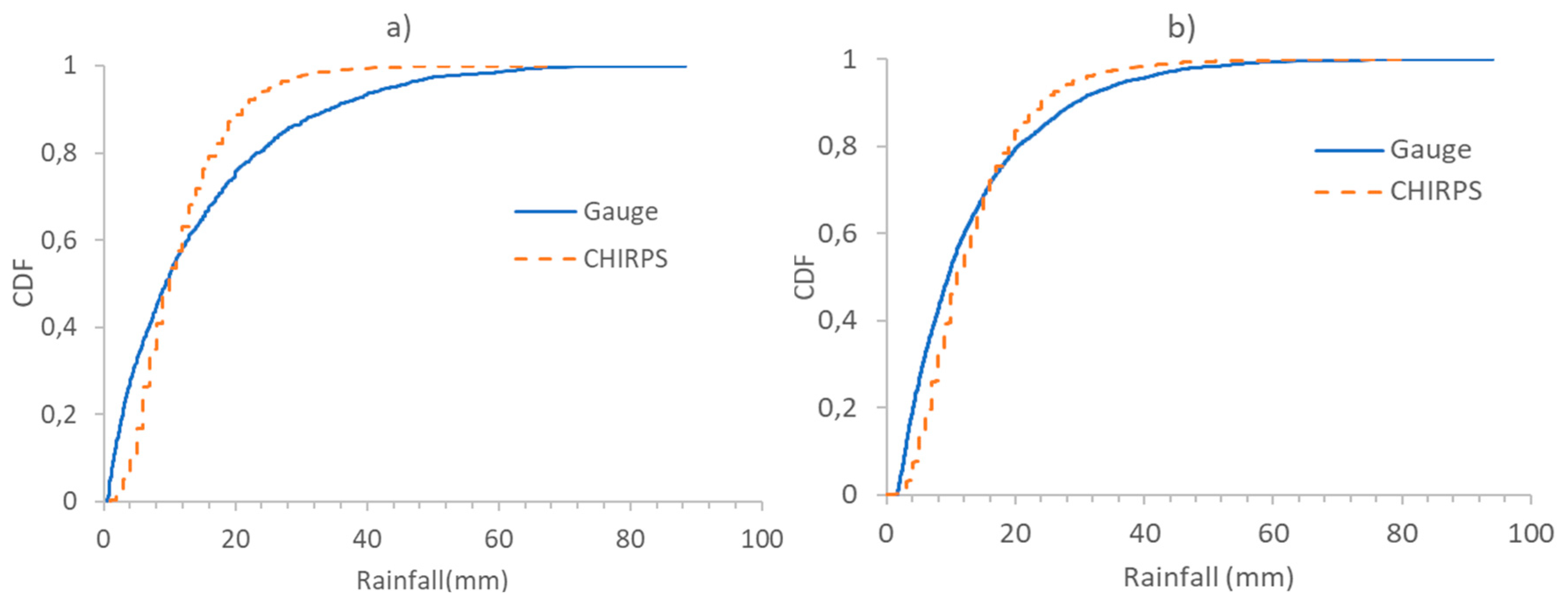
Assessment of Accuracy of Daily Rainfall Totals

The daily rainfall totals assessment of CHIRPS performance shows that for the highland regions it generally performs better than the lowland regions (

Table 5. Result of statistical continuous metrics analysis of performance of CHIRPS at the Beles Basin, comparing daily rainfall of the CHIRPS rainfall with ground gauge data of the lowland and highland stations during 2005–2015. N indicates the number of data pairs compared and $\overline{G}$ is the average daily rainfall (mm) of the gauge data.

Statistic	CHIRPS $\mathbf{Lowland}(\mathbf{N}=8027,\overline{\mathit{G}}=4.1)$	CHIRPS $\mathbf{Highland}(\mathbf{N}=\mathrm{12,352},\overline{\mathit{G}}=4.5)$
ME	−0.18 mm	−0.05 mm
MAE	4.52 mm	4.33 mm
NSE	0.12	0.03
Bias	0.82	0.99

). The ME of both regions is very small as compared to the average daily rainfall ($\overline{G}$), −0.18 mm for lowland and −0.05 mm for highland stations, but MAE is comparable with the average daily rainfall. CHIRPS daily rainfall on highland areas of Beles Basin shows lower random error (ME = −0.05 mm and MAE = 4.33 mm) as compared to lowlands (ME = −0.18 mm and MAE = 4.52 mm). The relative magnitude of the variance of the residuals compared to the variance of the observed rainfall performs better for lowlands than for highlands with NSE values of 0.12 and 0.03, respectively. The Bias shows that CHIRPS has a better agreement with gauge measurements in the highland regions compared to the lowland regions. The negative ME and a Bias less than one at both regions indicates that CHIRPS generally underestimates daily rainfall. It underestimates by 1% in the highlands and by 18% in the lowlands. Overall, CHIRPS estimates daily rainfall amounts better for the highlands than for the lowlands of the Beles Basin.

The CDFs of CHIRPS rainfall estimates and gauge measurements (Figure 3) show the representation of the distribution of daily rainfall well. For rain <10 mm/day in the lowlands and <20 mm/day in the highlands, CDFs of CHIRPS rainfall estimates are below rain gauge CDFs. This shows that CHIRPS underestimates the distribution of light rainfall events and overestimates the proportion of high intensity rainfall events in both regions. The CDFs of CHIRPS rainfall estimates also show that the proportion of heavy rainfall events is closer to gauge observations for the highlands than for the lowland areas. CDFs also revealed that 95% of daily gauge measurements were below 45 mm/day in the lowlands and below 37 mm/day in the highlands, whereas CHIRPS 95% of daily estimate proportion is below 25 mm/day and 30 mm/day, respectively. Overall, the CDFs show that the distribution of daily rainfall is well estimated by CHIRPS and relatively performs better in the highlands than lowlands.

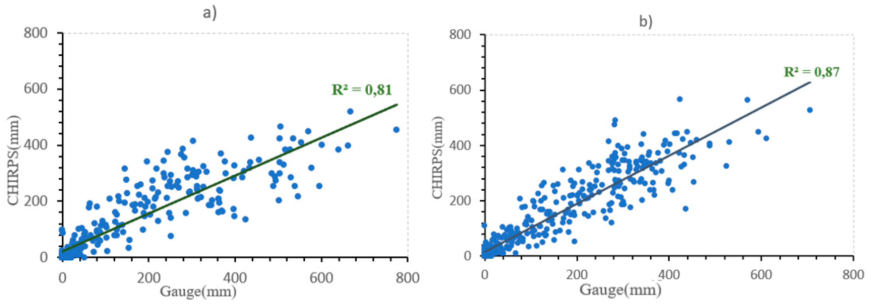
Assessment of Accuracy of Monthly Rainfall Totals

The performances of CHIRPS rainfall estimates improve at a monthly time scale (

Table 6. Performance statistics by comparing monthly rainfall of the CHIRPS rainfall with gauge data for the lowland and highland stations during 2005–2015 to evaluate performance of CHIRPS monthly rainfall at the Beles Basin. N indicates the number of data pairs compared and $\overline{G}$ is the average monthly rainfall (mm) of the gauge data.

	CHIRPS $\mathbf{Lowland}(\mathbf{N}=312,\overline{\mathit{G}}=126.1)$	CHIRPS $\mathbf{Highland}(\mathbf{N}=456,\overline{\mathit{G}}=144.9)$
ME	−28.09 mm	−1.87 mm
MAE	50.67 mm	33.15 mm
NSE	0.75	0.87
Biase	0.81	0.99

) compared to evaluations at a daily time scale (Table 5). As compared to the mean average monthly rainfall indicated, ME and MAE values show good performance of CHIRPS estimates. Monthly CHIRPS rainfall estimates perform better for highlands than for lowlands, underestimating by about 1.9 mm and 28.1 mm, respectively. NSE values of 0.75 and 0.87 for lowland and highland regions, respectively, show that CHIRPS rainfall estimates have good performance in accurately retrieving monthly rainfall. Bias also shows a better performance of monthly CHIRPS estimates for highlands than for lowlands. It negligibly underestimates monthly rainfall by 1% at highlands, and by 19% for the lowlands. Overall, Bias value <1 and a negative value of ME indicates that CHIRPS underestimates the monthly rainfall. Figure 4 shows the scatterplots of monthly observed rainfall and CHIRPS estimations, to further illustrate the performance in estimating monthly precipitation. It clearly shows that monthly variability of rainfall is better estimated in highland regions than in lowland regions. In general, the monthly and daily comparisons between the CHIRPS estimates and the rain gauge measurements (Table 5 and Table 6) confirm that CHIRPS estimates perform better in estimating rainfall at monthly than at daily time scale in the Beles Basin.

4.2. Spatio-Temporal Variability of Rainfall in Beles Basin

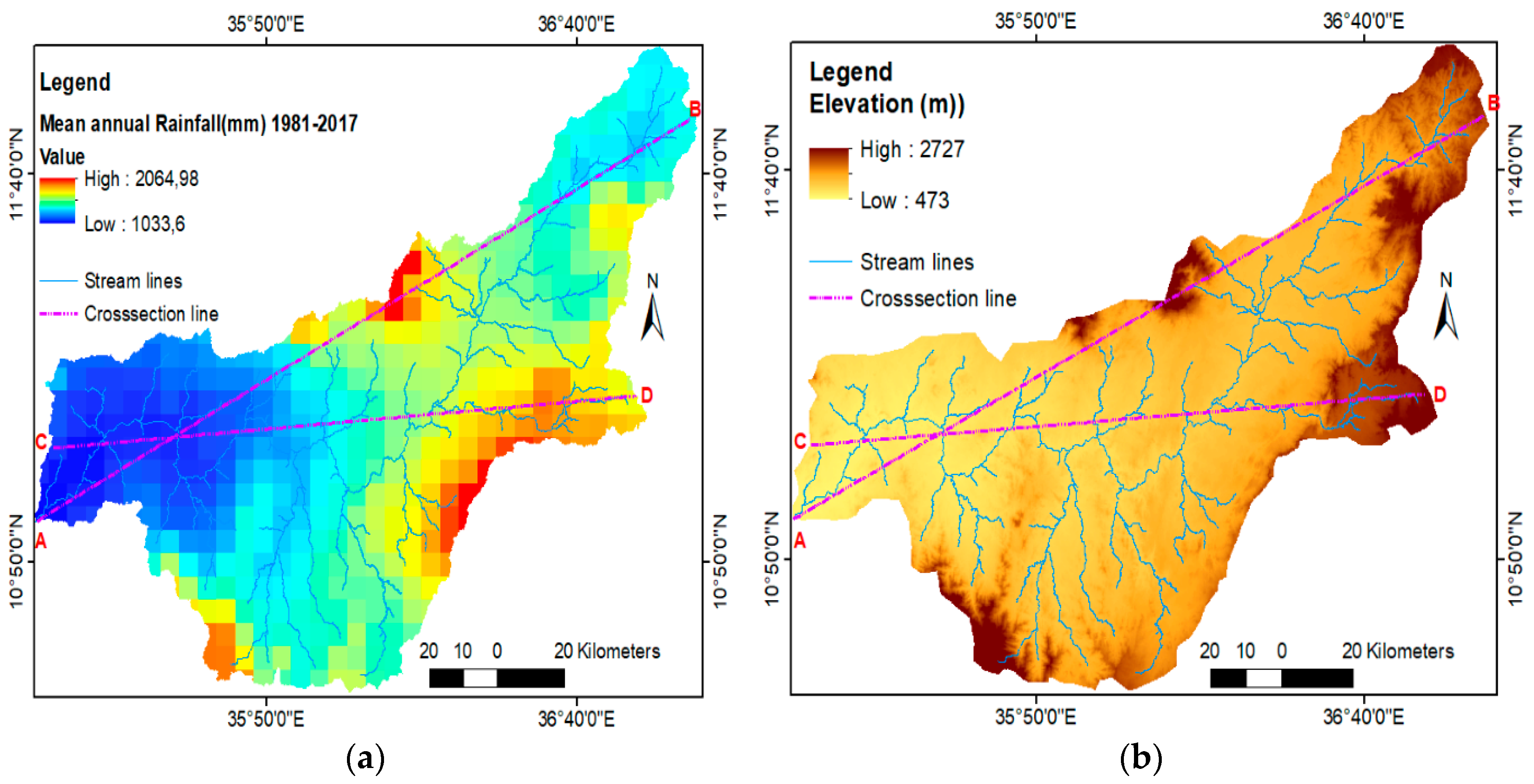
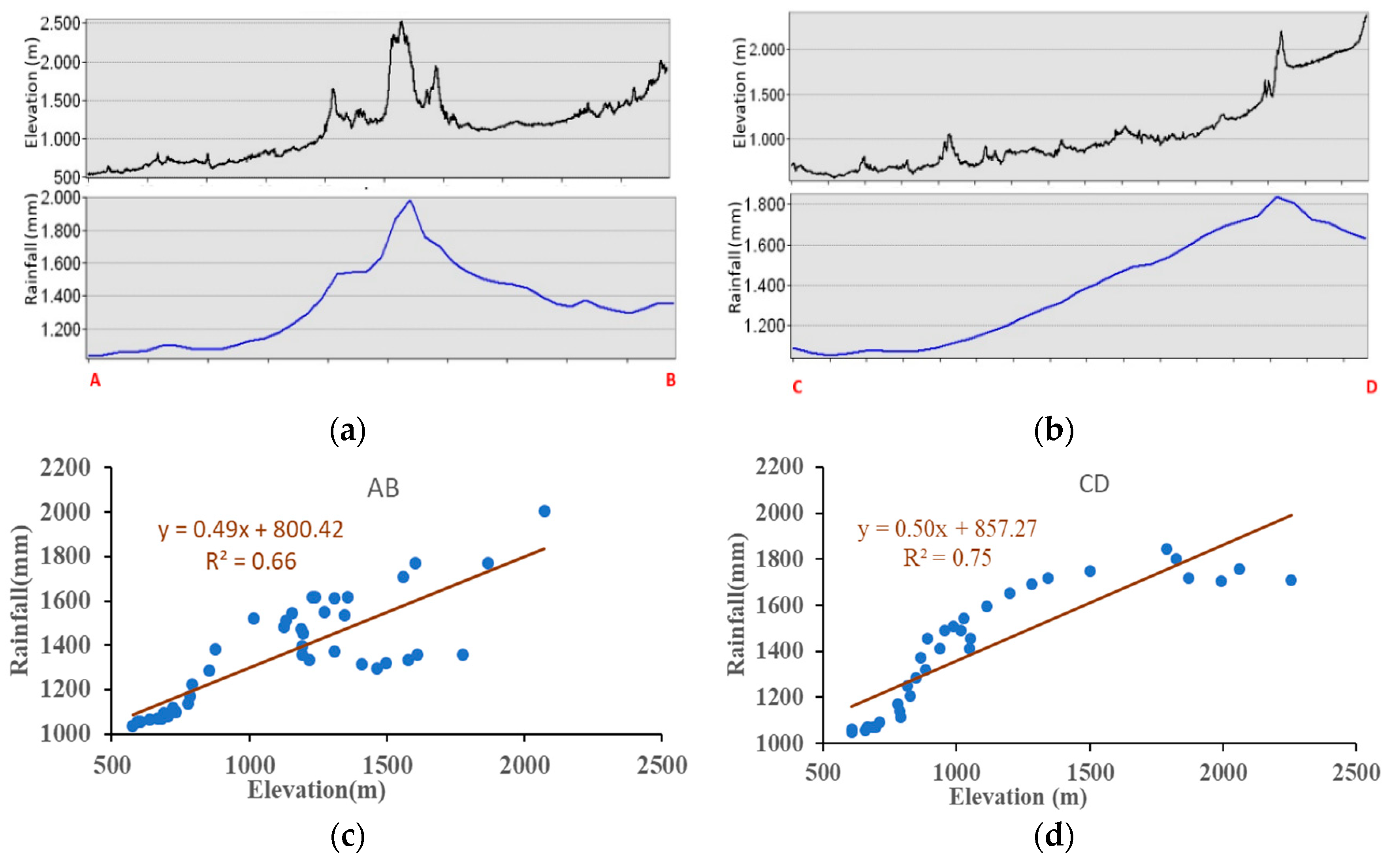
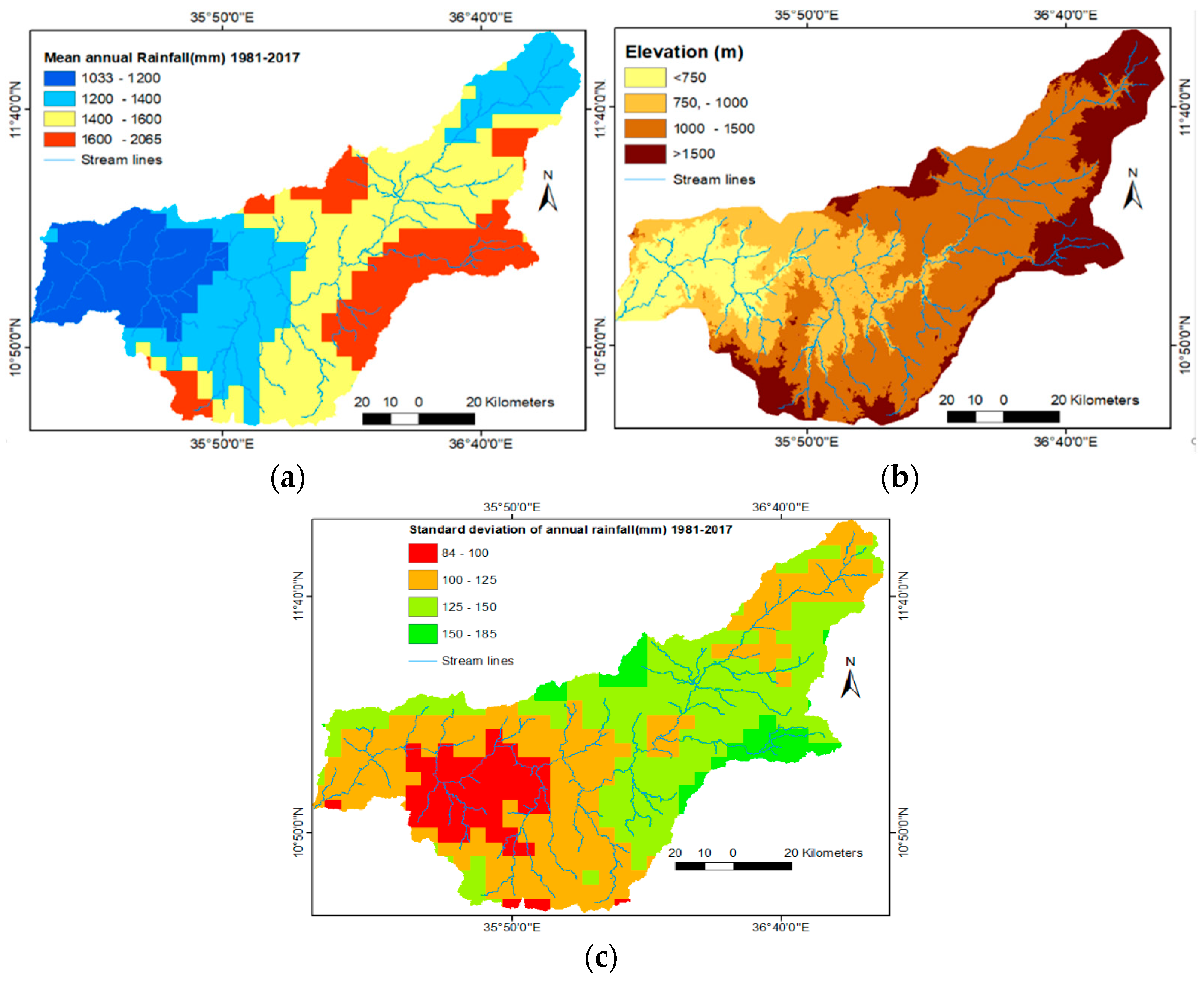
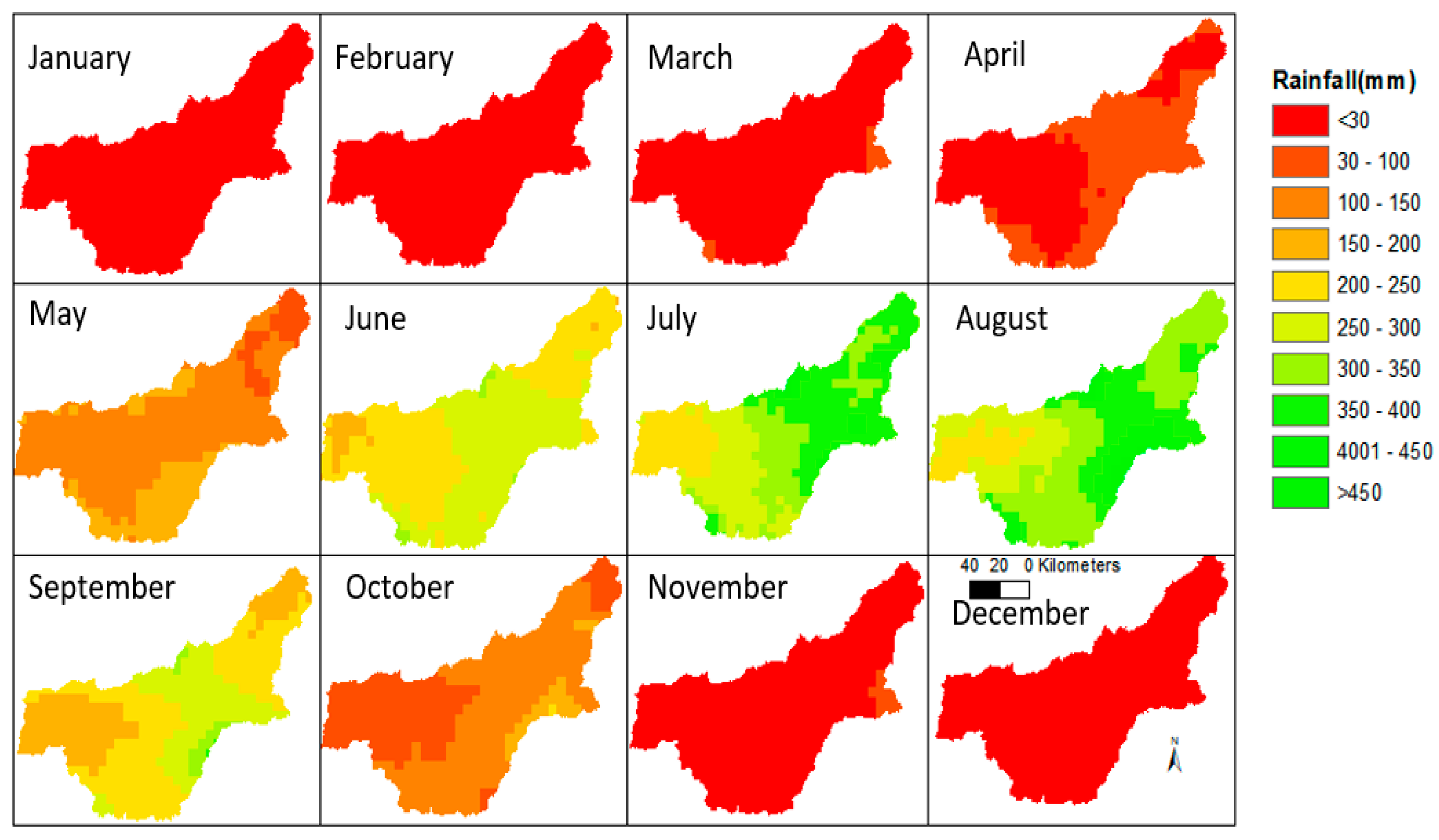
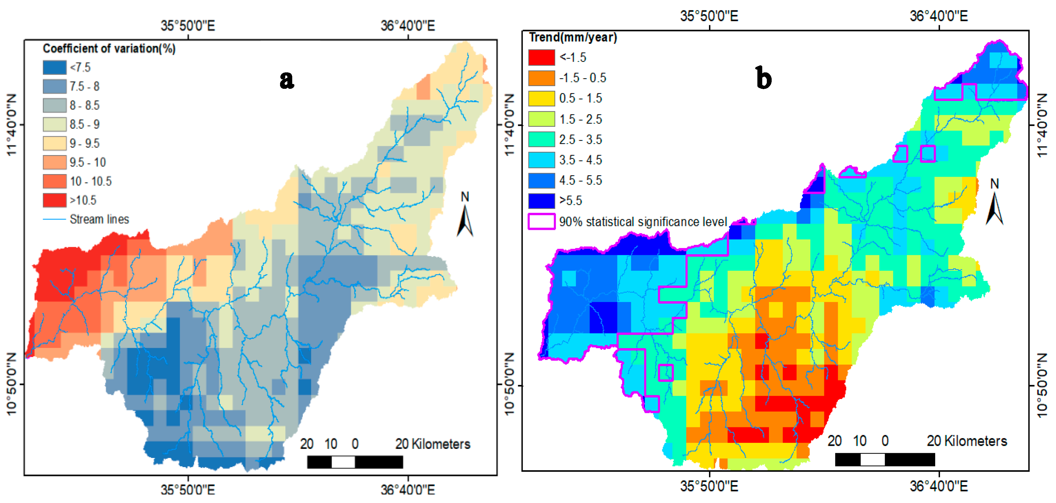
4.2.1. Spatial Variability of Rainfall

Long term mean annual CHIRPS rainfall estimates for 37 years in the Beles Basin shown in Figure 5 range between 1033 mm and 2091 mm, which indicates high spatial variability of rainfall. The highest annual rainfall values (about 2000 mm) were observed around Belaya mountain peaks (central north), along the Tana escarpment (southeastern basin boundary) and around the highlands of Wonberma (southwest) (Figure 5). The western lowland area of the Beles Basin is the driest region receiving the lowest annual rainfall amount (about 1100 mm). The central lowland areas between the Belaya mountain peak and Tana escarpment receive moderate rainfall. It is clear that there is a significant increasing trend of rainfall occurrence with elevation increases (Figure 6). This pattern is not well pronounced at the northeast corner of the basin although elevation is higher. The scatter plot between elevation and annual rainfall (Figure 6) shows that the rate of increase of mean annual rainfall with elevation is 50 mm per 100 m for the SW-NE (AB) and W-E (CD) transects.

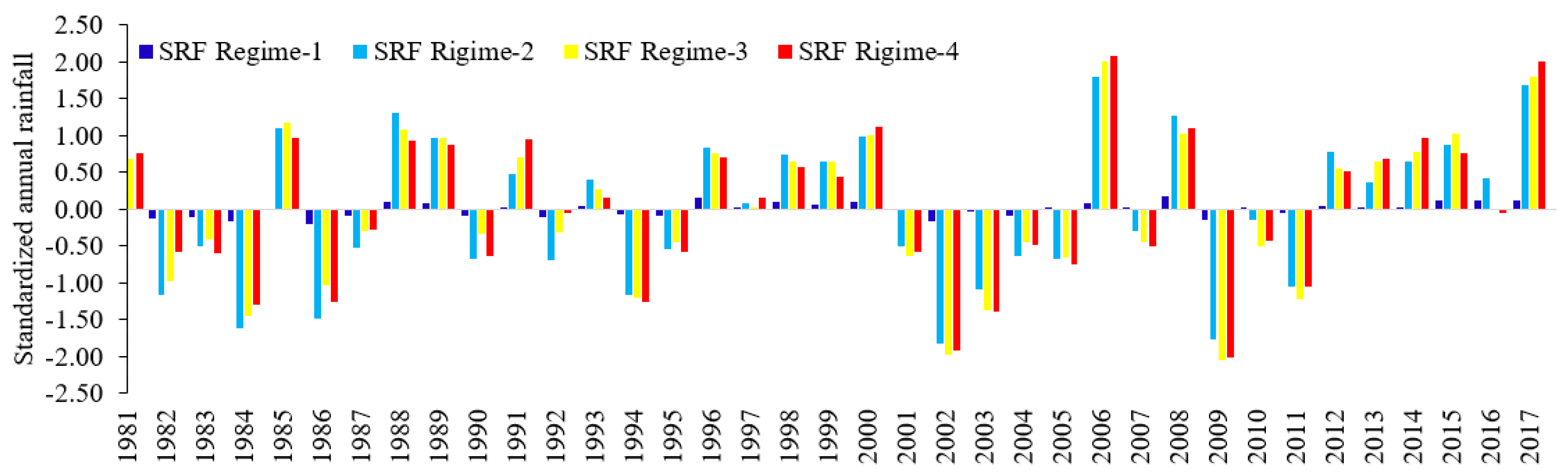
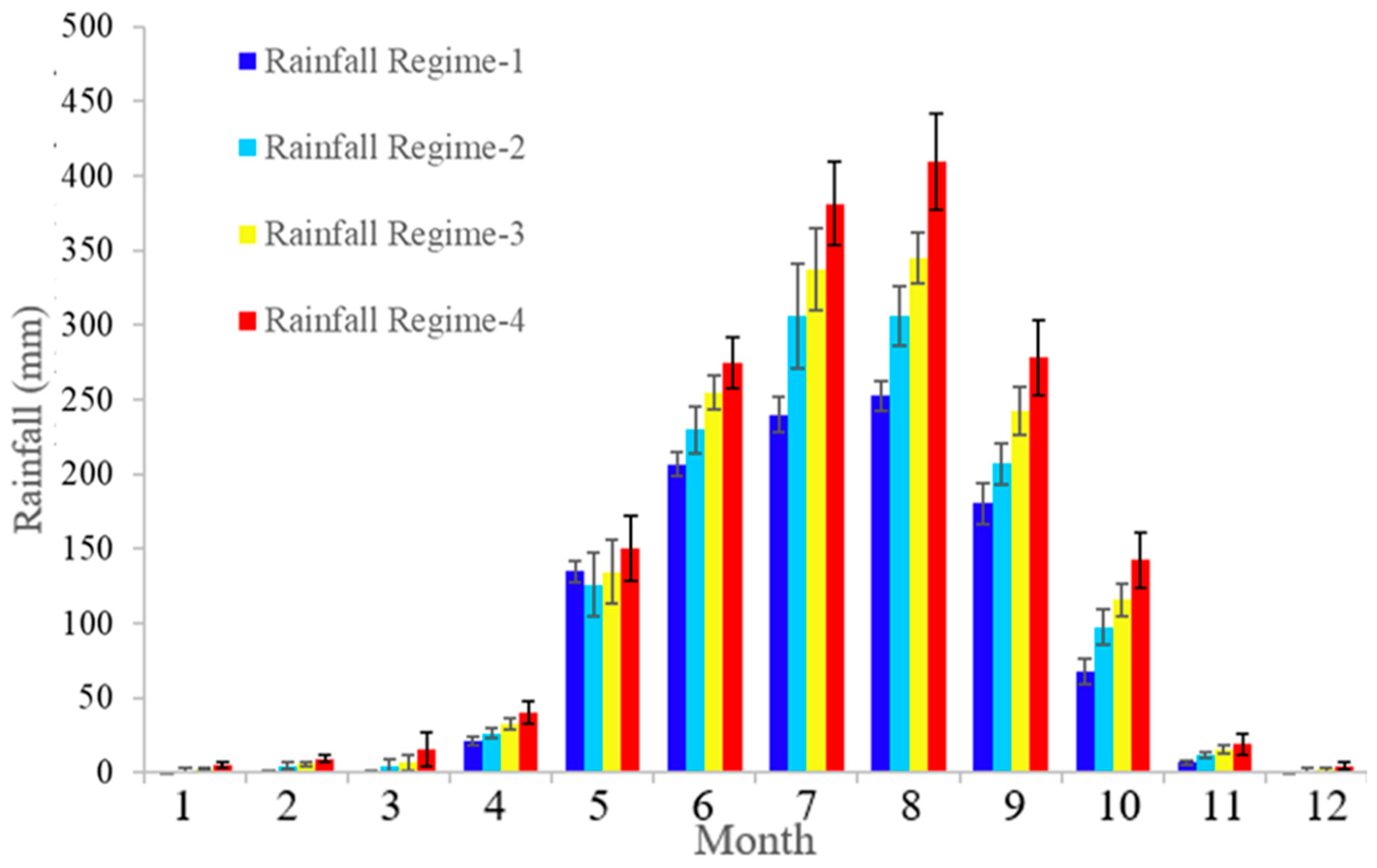
4.2.2. Spatio-Temporal Variability of Rainfall in Beles Basin

Long-term mean annual rainfall (37 years 1981–2017) from CHIRPS estimates were classified into four rainfall regime zones: 1033–1200 mm as regime-1, 1200–1400 mm as regime-2, 1400–1600 mm as regime-3 and 1600–2065 mm as regime-4. Each rainfall regime zone is spatially highly correlated to an elevation zone (Figure 7). Inter-annual variability of rainfall is highest in high rainfall regime zones (annual average standard deviation of 150–185 mm) around Belaya mountain and Tana escarpment and it is lowest at low rainfall regime zones in lowland parts of the basin (annual average standard deviation of 84–100 mm).

Figure 8 shows standardized anomalies of annual rainfall for each of the four rainfall regime zones. During the period 1981–2017, the proportion of both negative and positive anomalies of rainfall is observed. The interannual variability of each rainfall regime zone has a similar trend but the variability is much higher for high rainfall regime zones. Widespread low normal rainfall was experienced at all rainfall regime zones in 1982, 1984, 1986, 1994, 2002, 2003, 2009 and 2011 across the basin. Strongly positive anomalies for annual rainfall occurred in 2006 and 2017, receiving unusually high precipitation. The standardized annual rainfall shows that the reappearance of drought years seems likely to occur every 8 to 10 years and persistence with subsequent years of negative/positive anomalies.

Monthly zonal rainfall (Figure 9) was obtained by averaging the rainfall of each month in each rainfall regime zone (Figure 7). All four regime zones had wet conditions mainly in the months of June, July, August and September and dry conditions in November, December, January, February and March. Long-term mean monthly rainfall (Figure 10) shows that June, July, August and September were the main rainy months (>80% of annual rainfall), while November, December, January, February and March were the driest months, whereas little rainfall was observed in April, May and October in some parts of the basin. Rainfall starts in April (little shower) in the basin, except the western and northeastern part of the Beles Basin. In May, average rainfall reaches up to 200 mm except in the northeastern corner of the basin where rain starts mainly in June. Most of the study area receives the highest rainfall in August, except in the northeastern corner of the study area, where highest rainfall is obtained in July.

The coefficient of variation (CV) calculated for each pixel shown in Figure 11a visualizes the interannual spatial variability of annual rainfall in the Beles Basin. When the coefficient of variation (CV) value is greater than 10%, it indicates the standard deviation exceeds the mean rainfall. The high interannual variability (CV > 10%), experienced in low rainfall regions of the western downstream part of the basin, indicates that there is a greater contrast in annual rainfall values from year to year in this part of the basin. The smallest CV was observed over the south of the study area, showing relatively less interannual variations.

Spatio-temporal trends in decrease or increase of annual rainfall are observed in different zones. The trend statistics result (Figure 11b) has revealed that the low rainfall regime zones of the western and northeastern part of the study area have experienced a significant increase in rainfall trend, with an average mean annual rainfall around 5 mm/year during the period 1981–2017. Large part of the trend test statistics were not statistically significant (p < 0.1). Even though there is no statistically significant (p < 0.1) trend, decreasing trends of annual rainfall were observed in the study area. The southcentral part of the study area is marked by a slight decreasing trend of mean annual rainfall in 1981–2017. The dry regions of the western part of the study area showed statistically significant increasing trends, which implies that these areas were becoming wetter in the considered period.

The coefficient of variation (CV) of monthly rainfall (Figure 12) represents the temporal variability of monthly rainfall in Beles Basin. The high inter-monthly variability (CV > 50%) experienced in March, April and November with the highest CV >90% observed for March in the central part of the study area. The rainy months (June, July, August and September) show small coefficient of variation (<20%). In May, the eastern part of the study area experienced higher CV than the western part.

5. Discussion

A combination of high POD, FBI and HSS and a low FAR shows the good detection capability of satellite rainfall estimates. Table 4 shows that CHIRPS rainfall product slightly overestimates the occurrence of rainy days for lowlands (POD [0.72] and FBI [1.04]) and underestimates the occurrence of rainy days for highland regions (POD [0.67] < 1 and FBI [0.91] >1) of the Beles Basin. Compared to the previous study in the nearby region [8] (with POD ranging from 0.54 to 0.6 and FBI ranges from 0.70 to 0.87), our result showed good performance of the CHIRPS rainfall product. CHIRPS relies on a fixed TIR cloud coldness duration (CCD) threshold (235 K) [25] (the threshold used in the algorithm is not spatially and temporally varying thresholds to compute the CCD that used to distinguish raining and non-raining clouds). Therefore, the slight underestimation of the number of rainy days over the highland region could be attributed to the CCD threshold. The threshold may be too cold for regions where warm-rain processes dominate related to the warm orographic rain process. The overestimation of the occurrence of rainy days over the lowland region may be attributable to sub-cloud evaporation [21,24] (the dry atmosphere beneath the clouds could evaporate before reaching the surface, causing an overestimation of rainfall). The low sampling frequency and inaccuracies in disaggregating pentadal CCD totals to daily values [25] may also contribute to errors in the performance of CHIRPS detection capability of the occurrence of rainy days [24,30].

Evaluation of CHIRPS daily rainfall amounts (Table 5 and Figure 3) shows that CHIRPS generally underestimates daily rainfall moderately. Underestimation is larger for lowlands (ME [−0.18 mm] and MAE [4.52 mm]) than for highlands (ME = −0.05 mm and MAE = 4.33 mm) of the Beles Basin. In the Ethiopian highlands, previous studies [8,20] indicate CHIRPS’s underestimation could be attributed to: the areal mismatch of satellite data and gauge measurements (high rainfall intensities are commonly observed over smaller spatial domains than the pixel size of the CHIRPS), the retrieval algorithms in disaggregating pentadal data to daily values [8,25] and inaccuracies in measurements at gauge stations. The rainfall amounts estimated by CHIRPS are more accurate as the duration of the integration increase from days to months (Table 6 and Figure 4). This could be because of cancellation of errors of CHIRPS rainfall estimates as the duration of the integration increases [8,16,30,59] and error induced during disaggregating pentadal CCD totals to daily values is smaller at monthly time scale. Previous studies in the region [8,14,23,24,30,32,58], which consider the whole of our study area, the Beles Basin, as a lowland, showed that satellite rainfall estimates are better over the lowlands than over the highlands; however, our study demonstrates that at the local level within the Beles Basin, CHIRPS better estimated rainfall at highland regions than lowlands. The underestimation of CHIRPS rainfall product could be a result of shallow convection with warm cloud-top temperatures. This may lead to rainfall; however, if the cloud top is still relatively warm, as a result, CHIRPS may not detect rainfall because the cloud tops tend to be warmer than the TIR thresholds [8,14,24]. Overall, as compared to previous studies [8,16,17,32], the rainfall amounts estimated by CHIRPS perform well for Beles Basin. The good performance of CHIRPS could be because of the fact that PMW-based rainfall estimates from the TRMM-3B42 were used to calibrate the TIR images [8,25]. Bias-adjustment and inclusion of station data (mainly monthly) in CHIRPS estimate could also result in better rainfall estimation. The validation result revealed that performance of CHIRPS to estimate rainfall data at the Beles Basin is good as compared to studies in similar and nearby regions. Even where SREs perform quite poorly, it can provide reliable measures of relative rainfall amounts [14]. Therefore, from the perspective of applications, CHIRPS rainfall estimates can be used as a reliable source of data for hydrological applications that require rainfall data, especially at monthly and longer timescales.

Mean annual rainfall of the study area from CHIRPS ranges between 1033 and 2091 mm, and spatially highly controlled by topography (Figure 5). The rainfall in Ethiopia shows high spatial and temporal variability, likely attributable to geographical location and topography [60,61,62]. As such, rainfall distribution is influenced by topography due to orographic lifting [51]. The low mean annual rainfall in the northeastern part of the study area, despite the higher topography, could be because of the rain shadow effect [13,61] of Mount Belaya. The study area, as part of western Ethiopia, is identified as having a unimodal rainfall pattern which is caused by merging of wind systems coming from the Indian Ocean and from the Atlantic, to give continuous rain from March or April to October [13,45,63] and our results confirm this for the Beles Basin (Figure 9 and Figure 10), with the wettest months in June, July, August and September.

National and watershed level analysis of rainfall in Ethiopia using gauge data shows most parts of the country shows statistically insignificant trends in rainfall [43,63,64]; however, our analysis of trends at a basin level using CHIRPS rainfall data demonstrated some significant trends of rainfall that vary locally. A significant increasing trend of rainfall was identified in the driest lower part of Beles Basin (Figure 11). There is high spatial variability among the observed trends. Interannual rainfall variability and annual rainfall amounts are inversely related in the study area (Figure 11a). Previous studies in the region [52,55,63] have reported inverse relationship between CV and annual rainfall. The rainfall in the Beles Basin is characterized by moderate temporal interannual variability (Figure 11a) as compared to country level interannual variability with a high CV reaching up to 30% [64]. The low rainfall areas of the basin show high interannual variability, implying that in these regions there is a greater contrast in annual rainfall from year to year. This high interannual variability in turn indicates that, in such areas, water availability becomes more unpredictable. The higher coefficient of variation in March, April and to some extent in May (Figure 12) could indicate that sometimes the characteristics of rainfall in the Beles Basin might be of bimodal nature.

The meteorological drought years in the Beles Basin seem periodical with a reoccurrence of around 8 to 10 years (Figure 8). This pattern of variability of rainfall has been reported from nearby regions [43,60]. Since 1980, Ethiopia at country level experienced severe drought events in 1983–1985, 1988, 2000, 2002–2003, 2006, 2011 and 2015 [64]. Similarly, our study area also experienced most of these drought events (Figure 8) except years 1988, 2000, 2006 and 2015. In addition 1986, 1994 and 2009 were also localized drought years in Beles Basin. Extremely dry years in the country significantly affected the agricultural sector. Understanding the pattern of rainfall variability is essential because negative rainfall trends mostly result in a higher probability of droughts that have historically affected millions of people in Ethiopia [56,63,64]. It has been reported that the interannual variability of rainfall in the region could be under the influence of El Niño–Southern Oscillation (ENSO), and the Indian Ocean Sea Surface Temperature (SST) [43,52,65,66]. ENSO phenomena periodicities ranging from seasonal to about 8 years have been reported on East African region [67,68]. Therefore, periodical reoccurrence of dry and wet years at every 8 to 10 years could be associated with this regional climate index.

6. Conclusions

The characteristics of rainfall in the Beles Basin are not well known due to lack of adequately distributed meteorological stations. In this study, the spatial and temporal variability of rainfall has been analyzed using CHIRPS data after local validation. The validation results revealed that the CHIRPS rainfall product performed well at identifying rainfall days and estimating rainfall totals as compared to previous regional studies. Our work demonstrates that the performance of the CHIRPS product can vary locally at small basin level (capabilities vary in different climatic areas). It confirms the importance of a site-specific validation before using satellite rainfall products for different applications as has been recommended by previous works. It also shows that satellite rainfall estimates have different limitations over the different climatic regions and topographic conditions.

The spatio-temporal analysis of this study highlights the high spatial and temporal variability of rainfall. Rainfall has higher spatial dependence in the Beles river basin. The distribution and variability of mean annual rainfall has a key role on water availability, vegetation distribution, planning farming practices and assessment of desertification. In comparison to point-based gauge measurements, improved satellite rainfall estimations could truly represent spatial rainfall variability of this continuous geographical phenomenon. The information of interannual variability, trend and spatial distribution of rainfall using CHIRPS will help develop a better decision support system in the Beles Basin, where in the past decades, a lot of development activities have been done without a good understanding of the hydrology of the basin, due to lack of good quality gauge data. This understanding will help in hydrological investigations, water resources and energy development activities in the Beles Basin. Our study demonstrates that in areas where there is a scarcity of rain gauges, satellite rainfall products such as CHIRPS which provides temporally and spatially more complete data than rain gauges can help for better decision making by giving an option to understand the space-time variability of rainfall characteristics.

References

1. Awulachew, S.B.; Denekew, A.; Loulseged, Y.M.; Loiskandi, W.; Ayana, M.; Alamirew, T. IWMI Water Resources and Irrigation Development in Ethiopia; Working Paper 123; IWMI: Colombo, Sri Lanka, 2007. [Google Scholar]
2. Iqbal, M.F.; Athar, H. Validation of satellite based precipitation over diverse topography of Pakistan. Atmos. Res. 2018, 201, 247–260. [Google Scholar] [CrossRef]
3. Fenta, A.A.; Kifle, A.; Gebreyohannes, T.; Hailu, G. Spatial analysis of groundwater potential using remote sensing and GIS-based multi-criteria evaluation in Raya Valley, northern Ethiopia. Hydrogeol. J. 2015, 23, 195–206. [Google Scholar] [CrossRef]
4. Frisvold, G.B.; Murugesan, A. Use of Weather Information for Agricultural Decision Making. Weather Clim. Soc. 2013, 5, 55–69. [Google Scholar] [CrossRef]
5. Billi, P.; Alemu, Y.T.; Ciampalini, R. Increased frequency of flash floods in Dire Dawa, Ethiopia: Change in rainfall intensity or human impact? Nat. Hazards 2015, 76, 1373–1394. [Google Scholar] [CrossRef]
6. Maidment, R.I.; Allan, R.P.; Black, E. Recent observed and simulated changes in precipitation over Africa. Geophysical. Res. Lett. 2015, 42, 8155–8164. [Google Scholar] [CrossRef]
7. Thiemig, V.; Rojas, R.; Zambrano-Bigiarini, M.; Levizzani, V.; De Roo, A. Validation of Satellite-Based Precipitation Products over Sparsely Gauged African River Basins. J. Hydrometeorol. 2012, 13, 1760–1783. [Google Scholar] [CrossRef]
8. Fenta, A.A.; Yasuda, H.; Shimizu, K.; Ibaraki, Y.; Haregeweyn, N.; Kawai, T.; Belay, A.S.; Sultan, D.; Ebabu, K. Evaluation of satellite rainfall estimates over the Lake Tana basin at the source region of the Blue Nile River. Atmos. Res. 2018, 212, 43–53. [Google Scholar] [CrossRef]
9. Katsanos, D.; Retalis, A.; Michaelides, S. Validation of a high-resolution precipitation database (CHIRPS) over Cyprus for a 30-year period. Atmos. Res. 2016, 169, 459–464. [Google Scholar] [CrossRef]
10. Washington, R.; Harrison, M.; Conway, D.; Black, E.; Challinor, A.; Grimes, D.; Jones, R.; Morse, A.; Kay, G.; Todd, M. African Climate Change: Taking the Shorter Route. Bull. Am. Meteorol. Soc. 2006, 87, 1355–1366. [Google Scholar] [CrossRef]
11. Rivera, J.A.; Marianetti, G.; Hinrichs, S. Validation of CHIRPS precipitation dataset along the Central Andes of Argentina. Atmos. Res. 2018, 213, 437–449. [Google Scholar] [CrossRef]
12. Rientjes, T.; Haile, A.T.; Fenta, A.A. Diurnal rainfall variability over the Upper Blue Nile Basin: A remote sensing based approach. Int. J. Appl. Earth Obs. Geoinf. 2012, 21, 311–325. [Google Scholar] [CrossRef]
13. Haile, A.T.; Rientjes, T.; Gieske, A.; Gebremichael, M. Rainfall variability over mountainous and adjacent lake areas: The case of Lake Tana basin at the source of the Blue Nile River. J. Appl. Meteorol. Climatol. 2009, 48, 1696–1717. [Google Scholar] [CrossRef]
14. Dinku, T.; Ceccato, P.; Grover-Kopec, E.; Lemma, M.; Connor, S.J.; Ropelewski, C.F. Validation of satellite rainfall products over East Africa’s complex topography. Int. J. Remote Sens. 2007, 28, 1503–1526. [Google Scholar] [CrossRef]
15. Hirpa, F.A.; Gebremichael, M.; Hopson, T. Evaluation of High-Resolution Satellite Precipitation Products over Very Complex Terrain in Ethiopia. J. Appl. Meteorol. Climatol. 2010, 49, 1044–1051. [Google Scholar] [CrossRef]
16. Ayehu, G.T.; Tadesse, T.; Gessesse, B.; Dinku, T. Validation of new satellite rainfall products over the Upper Blue Nile Basin, Ethiopia. Atmos. Meas. Tech. 2018, 11, 1921–1936. [Google Scholar] [CrossRef]
17. Alemu, M.M.; Bawoke, G.T. Analysis of spatial variability and temporal trends of rainfall in Amhara region, Ethiopia. J. Water Clim. Chang. 2019. [Google Scholar] [CrossRef]
18. Hobouchian, M.P.; Salio, P.; García Skabar, Y.; Vila, D.; Garreaud, R. Assessment of satellite precipitation estimates over the slopes of the subtropical Andes. Atmos. Res. 2017, 190, 43–54. [Google Scholar] [CrossRef]
19. Bitew, M.M.; Gebremichael, M.; Ghebremichael, L.T.; Bayissa, Y.A. Evaluation of High-Resolution Satellite Rainfall Products through Streamflow Simulation in a Hydrological Modeling of a Small Mountainous Watershed in Ethiopia. J. Hydrometeorol. 2012, 13, 338–350. [Google Scholar] [CrossRef]
20. Dinku, T.; Hailemariam, K.; Maidment, R.; Tarnavsky, E.; Connor, S. Combined use of satellite estimates and rain gauge observations to generate high-quality historical rainfall time series over Ethiopia. Int. J. Climatol. 2014, 34, 2489–2504. [Google Scholar] [CrossRef]
21. Dinku, T.; Ceccato, P.; Connor, S.J. Challenges of satellite rainfall estimation over mountainous and arid parts of east Africa. Int. J. Remote Sens. 2011, 32, 5965–5979. [Google Scholar] [CrossRef]
22. Kidd, C. Satellite rainfall climatology: A review. Int. J. Climatol. 2001, 21, 1041–1066. [Google Scholar] [CrossRef]
23. Dinku, T.; Funk, C.; Grimes, D. The Potential of Satellite Rainfall Estimates for Index Insurance; The Earth Institute at Columbia University: New York, NY, USA, 2009; pp. 1–5. [Google Scholar]
24. Young, M.P.; Williams, C.J.R.; Chiu, J.C.; Maidment, R.I.; Chen, S.-H. Investigation of Discrepancies in Satellite Rainfall Estimates over Ethiopia. J. Hydrometeorol. 2014, 15, 2347–2369. [Google Scholar] [CrossRef]
25. Funk, C.; Peterson, P.; Landsfeld, M.F.; Pedreros, D.H.; Verdin, J.P.; Rowland, J.; Romero, B.E.; Husak, G.J.; Michaelsen, J.C.; Verdin, A.P. A Quasi-Global Precipitation Time Series for Drought Monitoring; U.S. Geological Survey Data Series; U.S. Geological Survey: Reston, VA, USA, 2014; Volume 832, p. 4.
26. Baez-Villanueva, O.M.; Zambrano-Bigiarini, M.; Ribbe, L.; Nauditt, A.; Giraldo-Osorio, J.D.; Thinh, N.X. Temporal and spatial evaluation of satellite rainfall estimates over different regions in Latin-America. Atmos. Res. 2018, 213, 34–50. [Google Scholar] [CrossRef]
27. Gao, F.; Zhang, Y.; Chen, Q.; Wang, P.; Yang, H.; Yao, Y.; Cai, W. Comparison of two long-term and high-resolution satellite precipitation datasets in Xinjiang, China. Atmos. Res. 2018, 212, 150–157. [Google Scholar] [CrossRef]
28. Lekula, M.; Lubczynski, M.W.; Shemang, E.M.; Verhoef, W. Validation of satellite-based rainfall in Kalahari. Phys. Chem. Earth 2018, 105, 84–97. [Google Scholar] [CrossRef]
29. Lakew, H.B.; Moges, S.A.; Asfaw, D.H. Hydrological Evaluation of Satellite and Reanalysis Precipitation Products in the Upper Blue Nile Basin: A Case Study of Gilgel Abbay. Hydrology 2017, 4, 39. [Google Scholar] [CrossRef]
30. Maidment, R.I.; Grimes, D.I.F.; Allan, R.P.; Greatrex, H.; Rojas, O.; Leo, O. Evaluation of satellite-based and model re-analysis rainfall estimates for Uganda. Meteorol. Appl. 2013, 20, 308–317. [Google Scholar] [CrossRef]
31. Zambrano-Bigiarini, M.; Nauditt, A.; Birkel, C.; Verbist, K.; Ribbe, L. Temporal and spatial evaluation of satellite-based rainfall estimates across the complex topographical and climatic gradients of Chile. Hydrol. Earth Syst. Sci. 2017, 21, 1295–1320. [Google Scholar] [CrossRef]
32. Dinku, T.; Funk, C.; Peterson, P.; Maidment, R.; Tadesse, T.; Gadain, H.; Ceccato, P. Validation of the CHIRPS satellite rainfall estimates over eastern Africa. Q. J. R. Meteorol. Soc. 2018, 114, 292–312. [Google Scholar] [CrossRef]
33. Usman, M.; Nichol, J.E.; Ibrahim, A.T.; Buba, L.F. A spatio-temporal analysis of trends in rainfall from long term satellite rainfall products in the Sudano Sahelian zone of Nigeria. Agric. For. Meteorol. 2018, 260–261, 273–286. [Google Scholar] [CrossRef]
34. Melesse, A.M.; Abtew, W.; Setegn, S.G. Nile River Basin: Ecohydrological Challenges, Climate Change and Hydropolitics; Springer: Cham, Switzerland, 2013; pp. 1–718. [Google Scholar]
35. Fenta, A.A.; Yasuda, H.; Shimizu, K.; Haregeweyn, N.; Kawai, T.; Sultan, D.; Ebabu, K.; Belay, A.S. Spatial distribution and temporal trends of rainfall and erosivity in the Eastern Africa region. Hydrol. Process. 2017, 31, 4555–4567. [Google Scholar] [CrossRef]
36. Muthoni, F.K.; Odongo, V.O.; Ochieng, J.; Mugalavai, E.M.; Mourice, S.K.; Hoesche-Zeledon, I.; Mwila, M.; Bekunda, M. Long-term spatial-temporal trends and variability of rainfall over Eastern and Southern Africa. Theor. Appl. Climatol. 2018, 137, 1869–1882. [Google Scholar] [CrossRef] [Green Version]
37. Rivera, T.; Marianetti, G.; Hinrichs, S.; Dinku, T.; Funk, C.; Peterson, P.; Maidment, R.I.; Tadesse, T.; Gadain, H.; Ceccato, P.; et al. Diurnal rainfall variability over the Upper Blue Nile Basin: A remote sensing based approach. Atmos. Res. 2018, 212, 1–718. [Google Scholar]
38. Zanardi, D. The Tana Beles resettlement project in Ethiopia Dario Zanardi. Évora I, Frias S (eds) Seminário sobre Ciências Sociais e Desenvolvimento em África. Cent. De Estud. Sobre África Desenvolv. 2011, 79–88. [Google Scholar]
39. Nyssen, J.; Fetene, F.; Dessie, M.; Alemayehu, G.; Sewnet, A.; Wassie, A.; Kibret, M.; Walraevens, K.; Derudder, B.; Nicolai, B.; et al. Persistence and changes in the peripheral Beles basin of Ethiopia. Reg. Environ. Chang. 2018, 18, 2089–2104. [Google Scholar] [CrossRef]
40. Clark, A.K.; Ratsey, J.; Wood, R.P.H. Feasibility studies for irrigation development in Ethiopia. Proc. Inst. Civ. Eng. Water Manag. 2013, 166, 219–230. [Google Scholar] [CrossRef]
41. Dessie, M.; Verhoest, N.E.C.; Admasu, T.; Pauwels, V.R.N.; Poesen, J.; Adgo, E.; Deckers, J.; Nyssen, J. Effects of the floodplain on river discharge into Lake Tana (Ethiopia). J. Hydrol. 2014, 519, 699–710. [Google Scholar] [CrossRef]
42. Annys, S.; Adgo, E.; Ghebreyohannes, T.; Van Passel, S.; Dessein, J.; Nyssen, J. Impacts of the hydropower-controlled Tana-Beles interbasin water transfer on downstream rural livelihoods (northwest Ethiopia). J. Hydrol. 2018, 569, 436–448. [Google Scholar] [CrossRef]
43. Wagesho, N.; Goel, N.K.; Jain, M.K. Temporal and spatial variability of annual and seasonal rainfall over Ethiopia. Hydrol. Sci. J. 2013, 58, 354–358. [Google Scholar] [CrossRef]
44. Worqlul, A.W.; Dile, Y.T.; Ayana, E.K.; Jeong, J.; Adem, A.A.; Gerik, T. Impact of climate change on streamflow hydrology in headwater catchments of the upper Blue Nile Basin, Ethiopia. Water 2018, 10, 120. [Google Scholar] [CrossRef] [Green Version]
45. Ayele, T.; Ahmed, N.; Ribbe, L.; Heinrich, J. Hydrological responses to land use / cover changes in the source region of the Upper Blue Nile Basin, Ethiopia. Sci. Total Environ. 2017, 575, 724–741. [Google Scholar]
46. Ciach, G.J.; Krajewski, W.F. On the estimation of radar rainfall error variance. Adv. Water Resour. 1999, 22, 585–595. [Google Scholar] [CrossRef]
47. Habib, E.; Krajewski, W.F. Uncertainty Analysis of the TRMM Ground-Validation Radar-Rainfall Products: Application to the TEFLUN-B Field Campaign. J. Appl. Meteorol. 2002, 41, 558–572. [Google Scholar] [CrossRef]
48. Ramsey, P.H. Statistical Methods in the Atmospheric Sciences. Technometrics 1996, 38, 402. [Google Scholar] [CrossRef]
49. Legates, D.R.; McCabe, G.J., Jr. Evaluating the sse of “Goodness of Fit” measures in hydrologic and hydroclimatic model validation. Water Resour. Res. 1999, 35, 233–241. [Google Scholar] [CrossRef]
50. Nash, E.; Sutcliffe, V. River flow forecasting through conceptual models part I—A discussion of principles. J. Hydrol. 1970, 10, 282–290. [Google Scholar] [CrossRef]
51. Arora, M.; Singh, P.; Goel, N.K.; Singh, R.D. Spatial distribution and seasonal variability of rainfall in a mountainous basin in the Himalayan region. Water Resour. Manag. 2006, 20, 489–508. [Google Scholar] [CrossRef]
52. Yasuda, H.; Panda, S.N.; Abd Elbasit, M.A.M.; Kawai, T.; Elgamri, T.; Fenta, A.A.; Nawata, H. Teleconnection of rainfall time series in the central Nile Basin with sea surface temperature. Paddy Water Environ. 2018, 16, 805–821. [Google Scholar] [CrossRef]
53. Rishmawi, K.; Prince, S.D.; Xue, Y. Vegetation Responses to Climate Variability in the Northern Arid to Sub-Humid Zones of Sub-Saharan Africa. Remote Sens. 2016, 8, 910. [Google Scholar] [CrossRef] [Green Version]
54. Suppiah, R.; Hennessy, K.J. Trends in total rainfall, heavy rain events and number of dry days in Australia, 1910–1990. Int. J. Climatol. 1998, 18, 1141–1164. [Google Scholar] [CrossRef]
55. Gedefaw, M.; Yan, D.; Wang, H.; Qin, T.; Girma, A.; Abiyu, A.; Batsuren, D. Innovative trend analysis of annual and seasonal rainfall variability in Amhara regional state, Ethiopia. Atmosphere 2018, 9, 326. [Google Scholar] [CrossRef] [Green Version]
56. Ravento, J.; Gonza, J.C.; Sa, J.R.; Cortina, J.; Lui, M.D.E. Spatial Analysis of Rainfall Trends in the Region of Valencia (East Spain). Int. J. Climatol. 2000, 1469, 1451–1469. [Google Scholar]
57. Yue, S.; Pilon, P.; Cavadias, G. Power of the Mann ± Kendall and Spearman’s rho tests for detecting monotonic trends in hydrological series. J. Hydrol. 2002, 259, 254–271. [Google Scholar] [CrossRef]
58. Forkel, M.; Carvalhais, N.; Verbesselt, J.; Mahecha, M.D.; Neigh, C.S.R.; Reichstein, M. Trend Change detection in NDVI time series: Effects of inter-annual variability and methodology. Remote Sens. 2013, 5, 2113–2144. [Google Scholar] [CrossRef] [Green Version]
59. Dembélé, M.; Zwart, S.J. Evaluation and comparison of satellite-based rainfall products in Burkina Faso, West Africa. Int. J. Remote Sens. 2016, 37, 3995–4014. [Google Scholar] [CrossRef] [Green Version]
60. Bewket, W.; Conway, D. A note on the temporal and spatial variability of rainfall in the drought-prone Amhara region of Ethiopia. Int. J. Climatol. 2007, 27, 1467–1477. [Google Scholar] [CrossRef]
61. Gebremichael, M.; Krajewski, W.F. Characterization of the temporal sampling error in space-time- averaged rainfall estimates from satellites. J. Geophys. Res. 2004, 109, 1–16. [Google Scholar] [CrossRef]
62. Diro, G.T.; Grimes, D.I.F.; Black, E.; O’Neill, A.; Pardo-Iguzquiza, E. Evaluation of reanalysis rainfall estimates over Ethiopia. ASHRAE Trans. 2017, 123, 162–173. [Google Scholar] [CrossRef]
63. Cheung, W.H.; Senay, B.; Singh, A. Trends and spatial distribution of annual and seasonal rainfall in Ethiopia. Int. J. Climatol. 2008, 1734, 1723–1734. [Google Scholar] [CrossRef]
64. Gummadi, S.; Rao, K.P.C.; Seid, J.; Legesse, G.; Kadiyala, M.D.M.; Takele, R. Spatio-temporal variability and trends of precipitation and extreme rainfall events in Ethiopia in 1980–2010. Theor. Appl. Climatol. 2017, 134, 2002–2003. [Google Scholar] [CrossRef] [Green Version]
65. Osman, Y.Z.; Shamseldin, A.Y. Southern sudan using elnino—Southern oscillation and southern sudan using el niño–southern oscillation and indian ocean sea surface temperature indices. Int. J. Climatol. 2002, 1878, 1861–1878. [Google Scholar] [CrossRef]
66. Fenta, A.A.; Tsunekawa, A.; Haregeweyn, N.; Poesen, J.; Tsubo, M.; Borrelli, P.; Panagos, P.; Vanmaercke, V.; Broeckx, J.; Yasuda, H.; et al. Land susceptibility to water and wind erosion risks in the East Africa region. Sci. Total Environ. 2019. [Google Scholar] [CrossRef]
67. Indeje, M.; Semazzi, F.H.M.; Ogallom, L.J. ENSO signals in East African rainfall seasons. Int. J. Climatol. 2000, 20, 19–46. [Google Scholar] [CrossRef]
68. Gleixnerm, S.; Keenlysidem, N.; Vistem, E.; Korecha, D. The El Niño effect on Ethiopian summer rainfall. Clim. Dyn. 2017, 49, 1865–1883. [Google Scholar] [CrossRef] [Green Version]
Figure 1. Location (a) and physiography of the Beles Basin, with rainfall gauging stations and surrounding areas of the Beles Basin (b) with 30 m resolution Digital Elevation Model from the Shuttle Radar Topographic Mission (SRTM) as a hillshade background. Lower photos show different landscapes in the basin; Belaya mountain (c) and Tana escarpment (d).
Remotesensing 11 02688 g001
Figure 2. Mean monthly rainfall (histogram) and standard deviation monthly rainfall (vertical lines) (2005–2015) for lowland (n = 4) and highland (n = 4) gauging stations in the Beles Basin.
Remotesensing 11 02688 g002
Figure 3. Daily Rainfall Cumulative Distribution Functions (CDFs) of CHIRPS estimates and gauge measurement: (a) for low land stations and (b) for highland station of the Beles Basin during 2005–2015.
Remotesensing 11 02688 g003
Figure 4. Scatter plot comparison of monthly rainfall, between rain gauge and CHIRPS satellite rainfall estimates for 2005–2015: (a) Lowland regions; (b) Highland regions.
Remotesensing 11 02688 g004
Figure 5. CHIRPS long-term mean annual rainfall (mm) from 1981 to 2017 (a) and Shuttle Radar Topography Mission (SRTM) 30 m Digital Elevation Model for Beles Basin (b).
Remotesensing 11 02688 g005
Figure 6. Long-term mean monthly rainfall and elevation along transect line (Figure 5) from A to B (a,c) and from C to D (b,d) and a scatter plot (c,d) of regression equation to determine rate of change of rainfall with elevation for each transect line AB and CD.
Remotesensing 11 02688 g006
Figure 7. Rainfall regime zones from long-term mean annual rainfall; zone-1: 1033–1200 mm, zone-2: 1200–1400 mm, zone-3: 1400–1600 mm, and zone-4: 1600–2065 mm (a). Elevation using Shuttle Radar Topography Mission Digital Elevation Model (STRM DEM) (b) and standard deviation of long-term annual rainfall (c).
Remotesensing 11 02688 g007
Figure 8. Standardized annual rainfall for each rainfall regime zone (Figure 7) in each year.
Remotesensing 11 02688 g008
Figure 9. Long-term mean monthly rainfall of the Beles Basin (histogram) and standard deviation of monthly rainfall (vertical lines) (1981–2017) over each rainfall regime zone (Figure 7); the color corresponds to a regime zone.
Remotesensing 11 02688 g009
Figure 10. Spatial distribution of long-term mean monthly rainfall of the Beles Basin (1981–2017).
Remotesensing 11 02688 g010
Figure 11. Spatial and temporal characteristics of rainfall during the period 1981–2017: (a) coefficient of variation, (b) trend (rate of change measured as the slope of linear trend in mm year−1), pink colored lines represent the 90% statistical significance level.
Remotesensing 11 02688 g011
Figure 12. Monthly coefficient of variation of rainfall during the period 1981–2017.
Remotesensing 11 02688 g012