Sequential PCA-based Classification of Mediterranean Forest Plants using Airborne Hyperspectral Remote Sensing


Abstract
:1. Introduction
2. Methodology
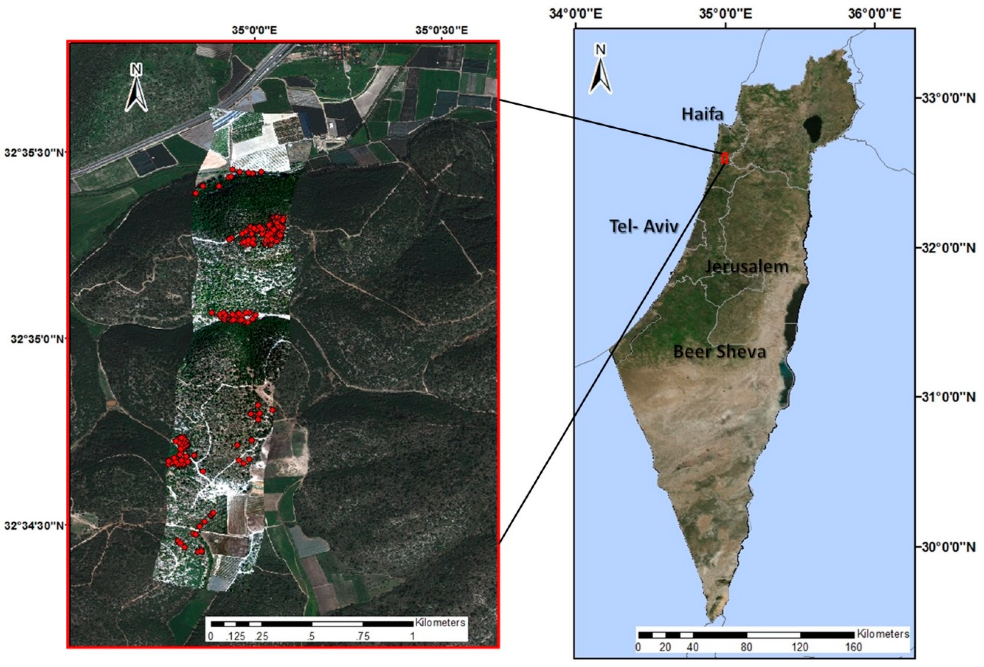
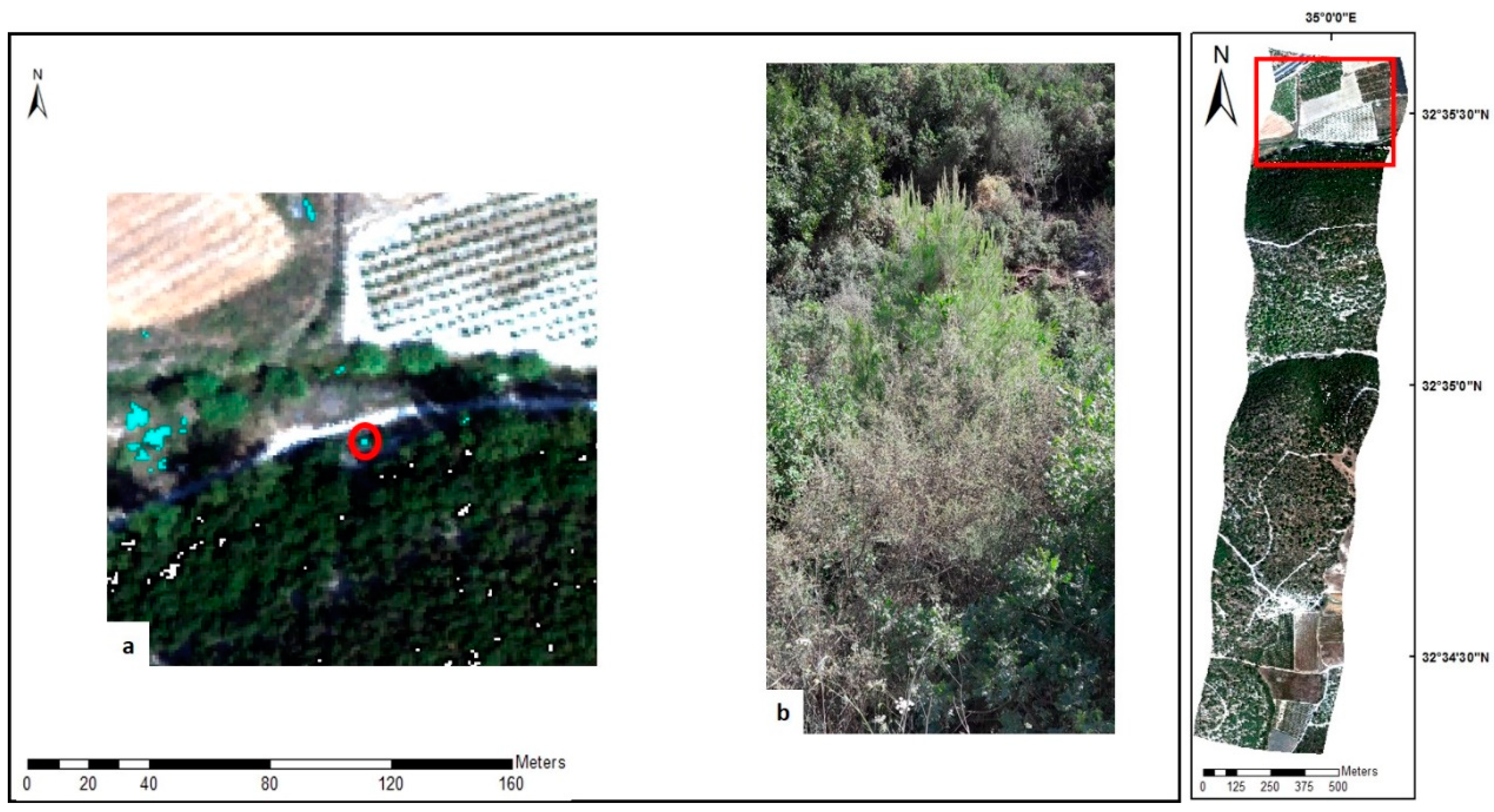
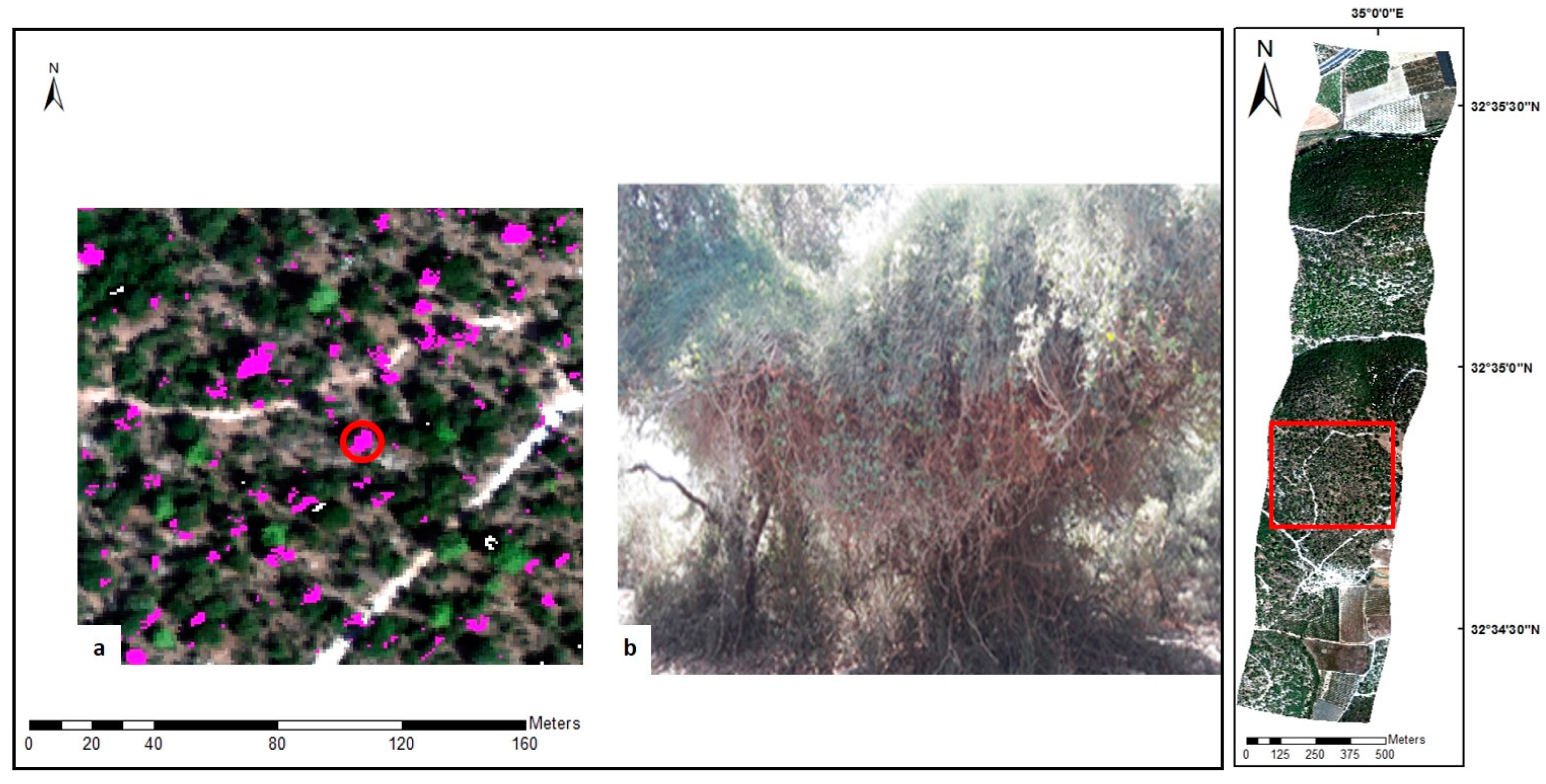
2.1. Research Site
2.2. Preprocessing
2.3. K-Means and ISODATA Classifiers
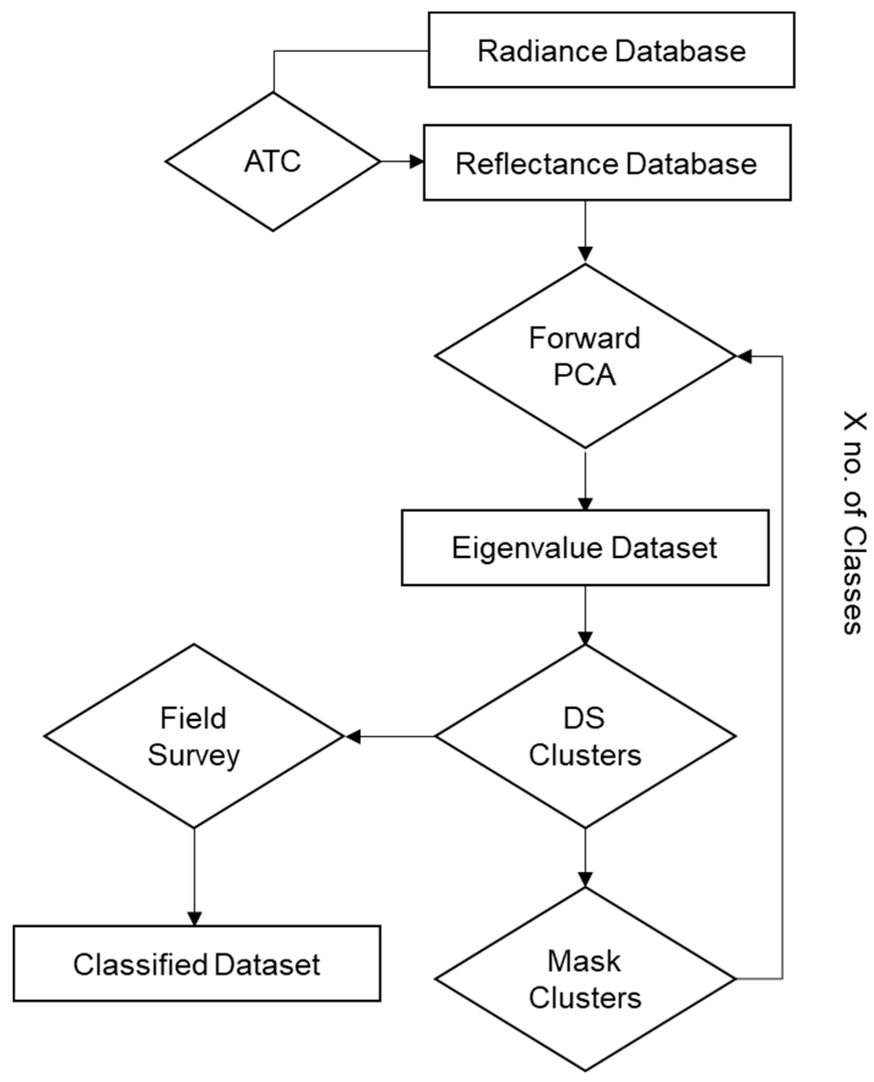
2.4. PCABC Processing
2.5. Validation Process
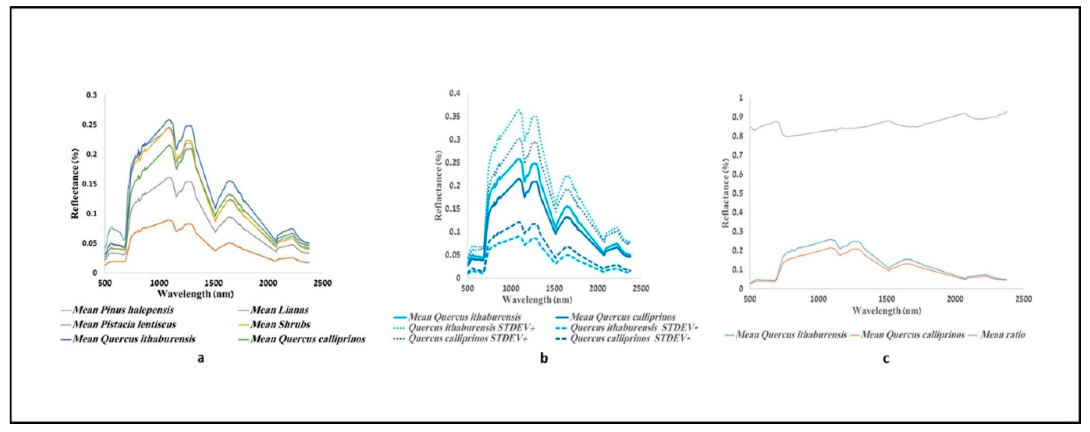
3. Results and Validation
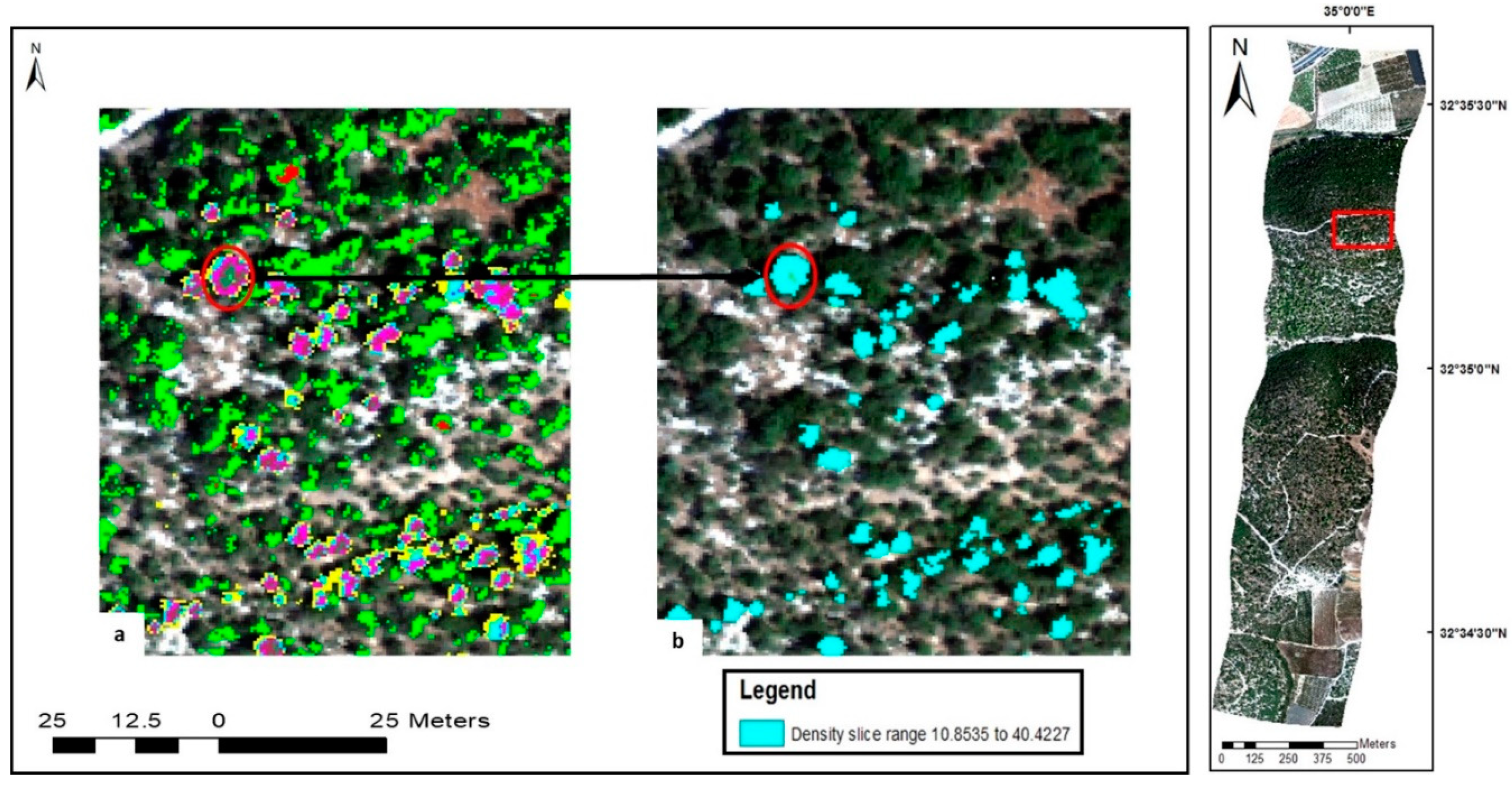
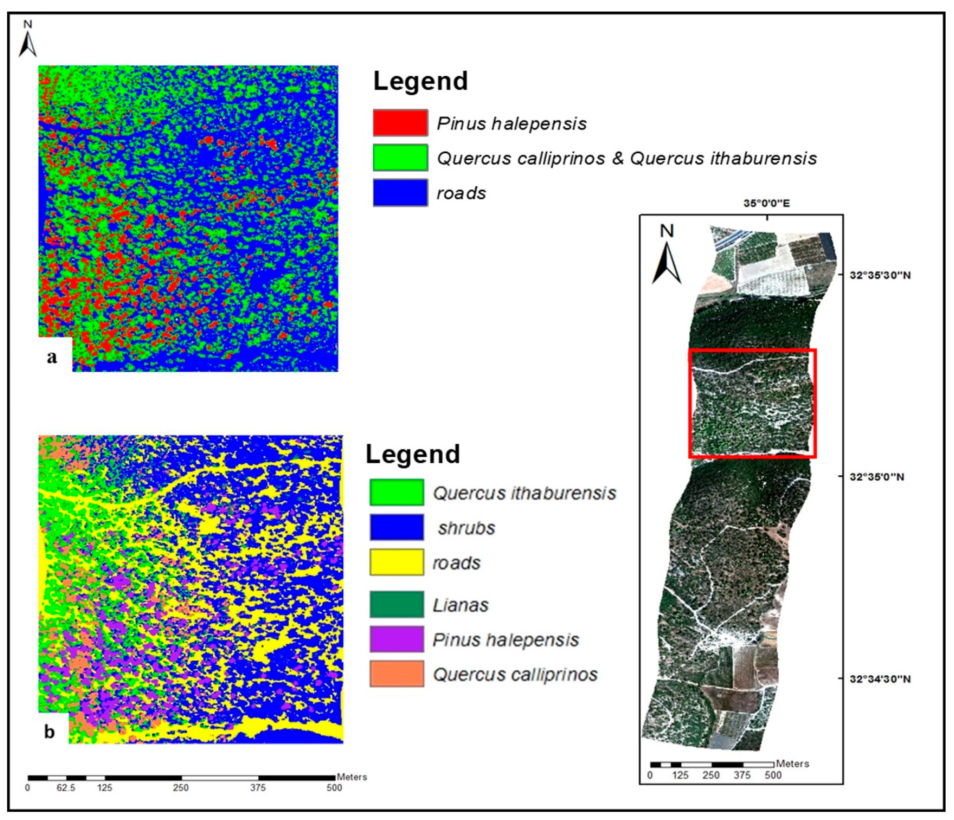
3.1. K-Means and ISODATA Results
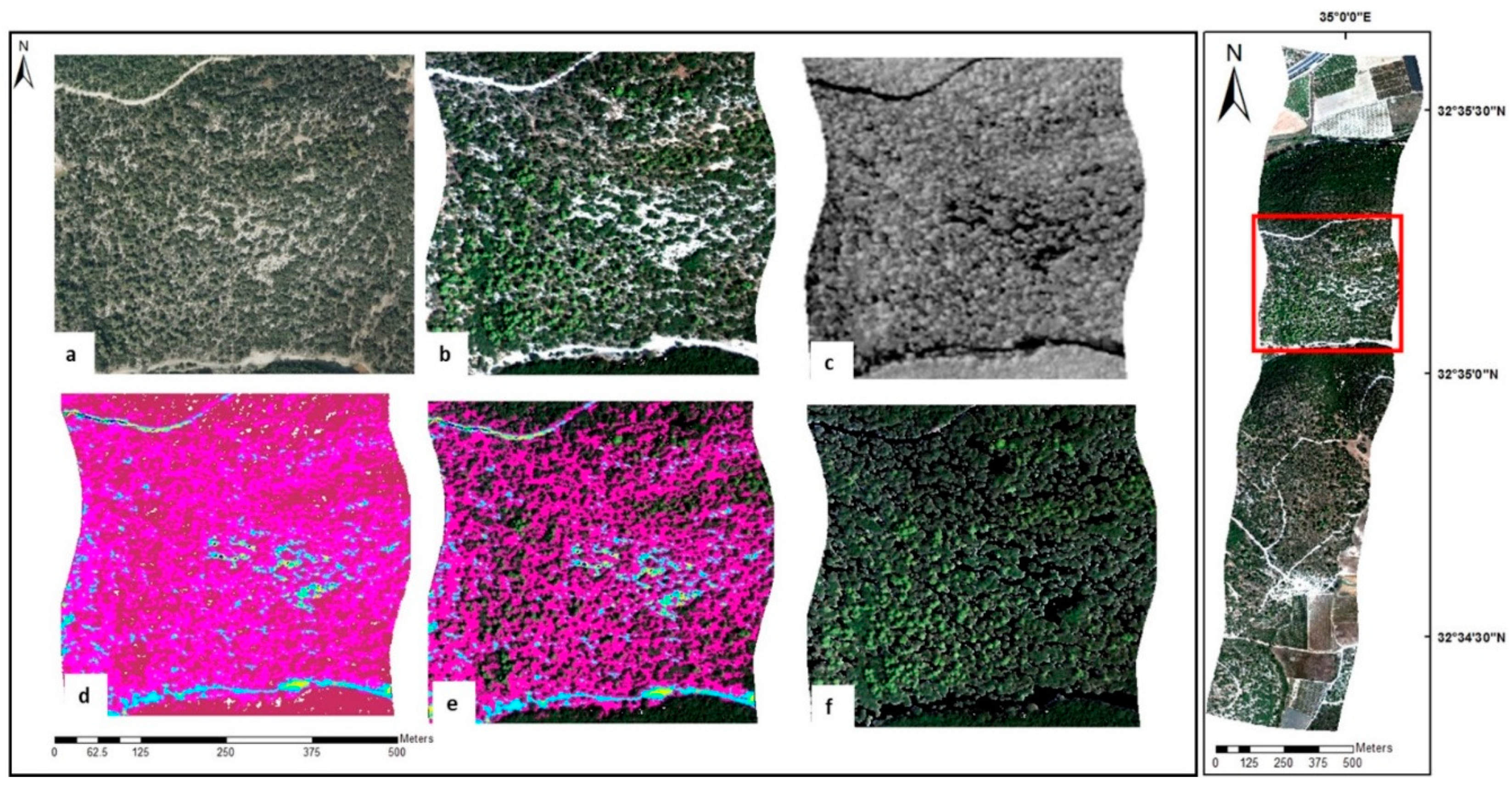
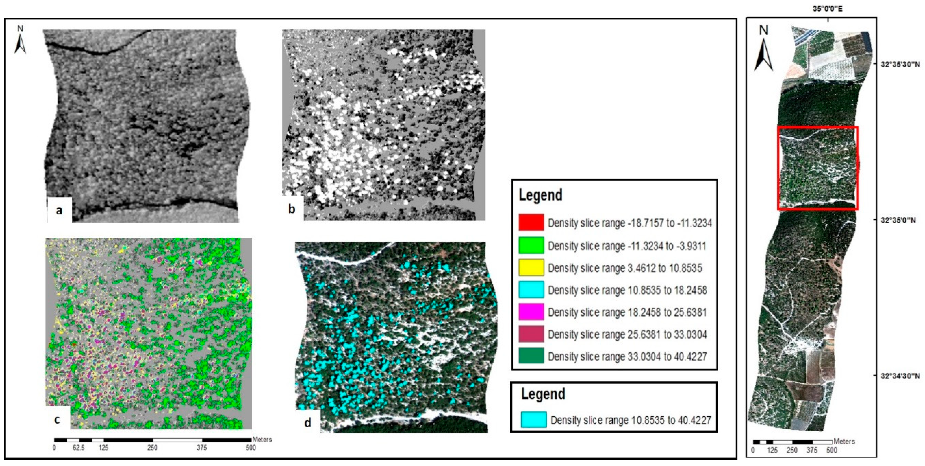
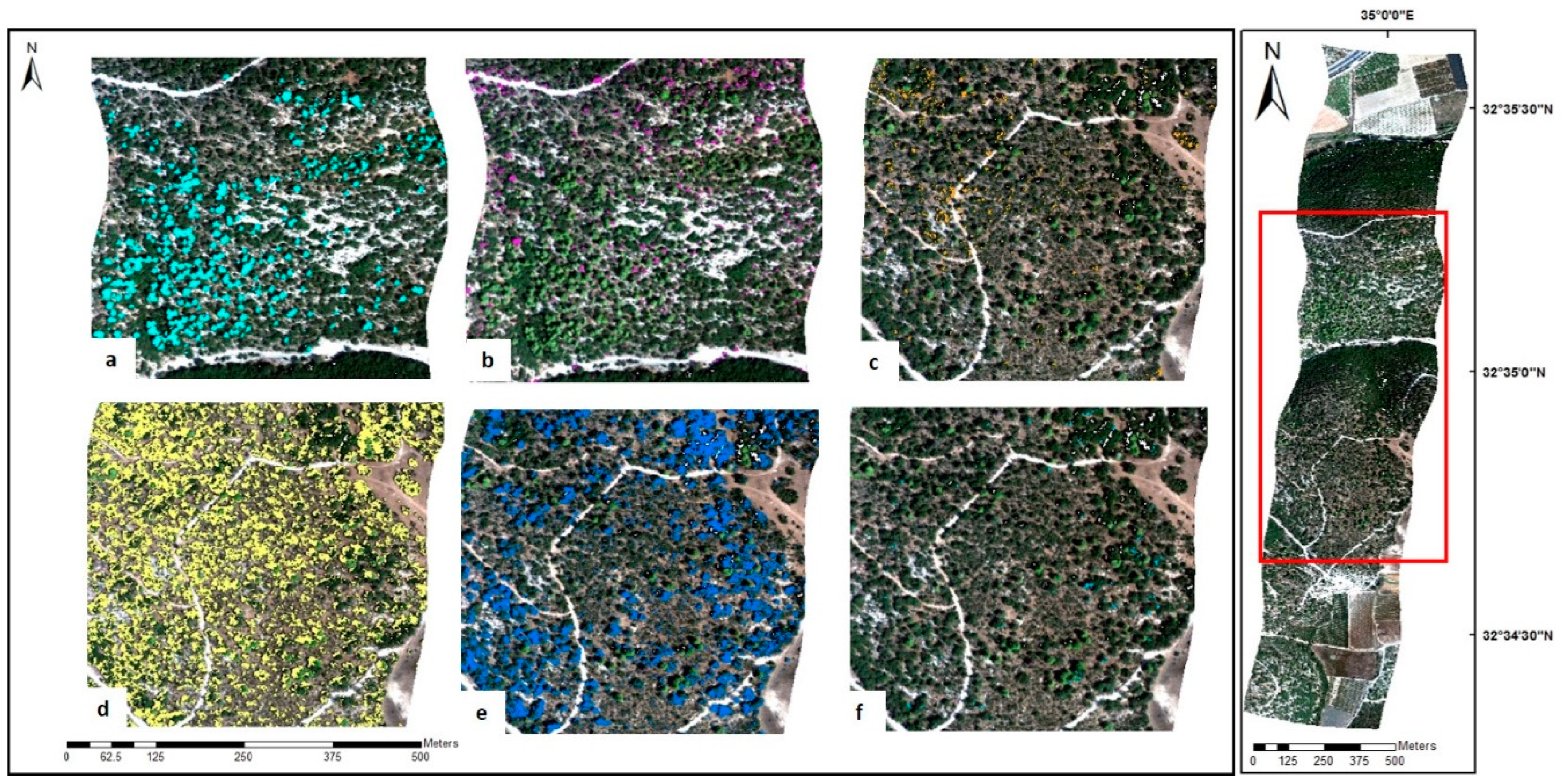
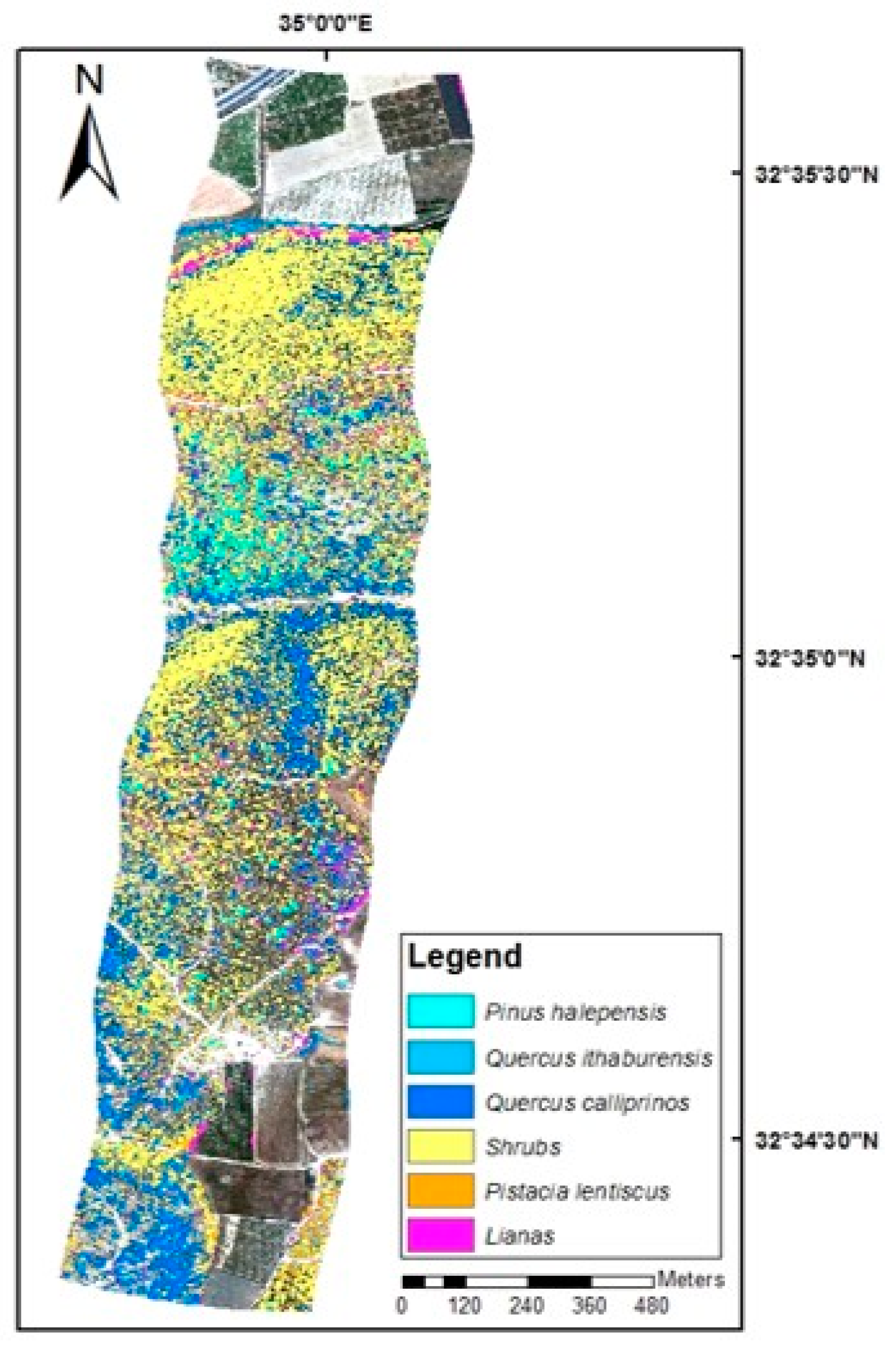
3.2. PCABC Results
4. Discussion
5. Summary and Conclusions
Author Contributions
Funding
Acknowledgments
Conflicts of Interest
References
- Asner, G.P.; Martin, R.E.; Anderson, C.B.; Knapp, D.E. Quantifying forest canopy traits: Imaging spectroscopy versus field survey. Remote Sens. Environ. 2015, 158, 15–27. [Google Scholar] [CrossRef]
- Ustin, S.L.; Roberts, D.A.; Gamon, J.A.; Asner, G.P.; Green, R.O. Using Imaging Spectroscopy to Study Ecosystem Processes and Properties. BioScience 2004, 54, 523–534. [Google Scholar] [CrossRef]
- Jaiswal, R.K.; Mukherjee, S.; Raju, K.D.; Saxena, R. Forest fire risk zone mapping from satellite imagery and GIS. Int. J. Appl. Earth Obs. Geoinf. 2002, 4, 1–10. [Google Scholar] [CrossRef]
- Carlson, K.M.; Asner, G.P.; Hughes, R.F.; Ostertag, R.; Martin, R.E. Hyperspectral Remote Sensing of Canopy Biodiversity in Hawaiian Lowland Rainforests. Ecosystems 2007, 10, 536–549. [Google Scholar] [CrossRef]
- Clark, M.L.; Roberts, D.A.; Clark, D.B. Hyperspectral discrimination of tropical rain forest tree species at leaf to crown scales. Remote Sens. Environ. 2005, 96, 375–398. [Google Scholar] [CrossRef]
- Francis, E.J.; Asner, G.P. High-Resolution Mapping of Redwood (Sequoia sempervirens) Distributions in Three Californian Forests. Remote Sens. 2019, 11, 351. [Google Scholar] [CrossRef]
- Peng, Y.; Fan, M.; Bai, L.; Sang, W.; Feng, J.; Zhao, Z.; Tao, Z. Identification of the Best Hyperspectral Indices in Estimating Plant Species Richness in Sandy Grasslands. Remote Sens. 2019, 11, 588. [Google Scholar] [CrossRef]
- Aslett, Z.; Taranik, J.V.; Riley, D.N. Mapping rock forming minerals at Boundary Canyon, Death Valey National Park, California, using aerial SEBASS thermal infrared hyperspectral image data. Int. J. Appl. Earth Obs. Geoinf. 2018, 64, 326–339. [Google Scholar] [CrossRef]
- Aitkenhead, M.J.; Black, H.I.J. Exploring the impact of different input data types on soil variable estimation using the ICRAF-ISRIC global soil spectral database. Appl. Spectrosc. 2018, 72, 188–198. [Google Scholar] [CrossRef]
- Cao, Z.; Wang, Q. Retrieval of leaf fuel moisture contents from hyperspectral indices developed from dehydration experiments. Eur. J. Remote Sens. 2017, 50, 18–28. [Google Scholar] [CrossRef]
- Carmon, N.; Ben-Dor, E. Mapping Asphaltic Roads’ Skid Resistance Using Imaging Spectroscopy. Remote Sens. 2018, 10, 430. [Google Scholar] [CrossRef]
- Carmon, N.; Ben-Dor, E. Rapid Assessment of Dynamic Friction Coefficient of Asphalt Pavement Using Reflectance Spectroscopy. IEEE Geosci. Remote Sens. Lett. 2016, 13, 721–724. [Google Scholar] [CrossRef]
- Gholizadeh, A.; Saberioon, M.; Ben-Dor, E.; Boruvka, L. Monitoring of selected soil contaminants using proximal and remote sensing techniques: Background, state-of-the-art and future perspectives. Crit. Rev. Environ. Sci. Technol. 2018, 48, 243–278. [Google Scholar] [CrossRef]
- Govil, H.; Gill, N.; Rajendran, S.; Santosh, M.; Kumar, S. Identification of new base metal mineralization in Kumaon Himalaya, India, using hyperspectral remote sensing and hydrothermal alteration. Ore Geol. Rev. 2018, 92, 271–283. [Google Scholar] [CrossRef]
- Homolová, L.; Malenovský, Z.; Clevers, J.G.; García-Santos, G.; Schaepman, M.E. Review of optical-based remote sensing for plant trait mapping. Ecol. Complex. 2013, 15, 1–16. [Google Scholar] [CrossRef]
- Houborg, R.; Fisher, J.B.; Skidmore, A.K. Advances in remote sensing of vegetation function and traits. Int. J. Appl. Earth Obs. Geoinf. 2015, 43, 1–6. [Google Scholar] [CrossRef]
- Kokaly, R.F.; Skidmore, A.K. Plant phenolics and absorption features in vegetation reflectance spectra near 1.66 μm. Int. J. Appl. Earth Obs. Geoinf. 2015, 43, 55–83. [Google Scholar] [CrossRef]
- Kopačková, V.; Ben-Dor, E.; Carmon, N.; Notesco, G. Modelling Diverse Soil Attributes with Visible to Longwave Infrared Spectroscopy Using PLSR Employed by an Automatic Modelling Engine. Remote Sens. 2017, 9, 134. [Google Scholar] [CrossRef]
- Kopačková, V.; Ben-Dor, E. Normalizing reflectance from different spectrometers and protocols with an internal soil standard. Int. J. Remote Sens. 2016, 37, 1276–1290. [Google Scholar] [CrossRef]
- Arroyo, L.A.; Pascual, C.; Manzanera, J.A. Fire models and methods to map fuel types: The role of remote sensing. For. Ecol. Manag. 2008, 256, 1239–1252. [Google Scholar] [CrossRef]
- Shoshany, M.; Svoray, T. Multidate adaptive unmixing and its application to analysis of ecosystem transitions along a climatic gradient. Remote Sens. Environ. 2002, 82, 5–20. [Google Scholar] [CrossRef]
- Wittenberg, L.; Malkinson, D.; Beeri, O.; Halutzy, A.; Tesler, N. Spatial and temporal patterns of vegetation recovery following sequences of forest fires in a Mediterranean landscape, Mt. Carmel Israel. Catena 2007, 71, 76–83. [Google Scholar] [CrossRef]
- Deng, J.S.; Wang, K.; Deng, Y.H.; Qi, G.J. PCA-based land-use change detection and analysis using multitemporal and multisensor satellite data. Int. J. Remote Sens. 2008, 29, 4823–4838. [Google Scholar] [CrossRef]
- Green, A.; Berman, M.; Switzer, P.; Craig, M. A transformation for ordering multispectral data in terms of image quality with implications for noise removal. IEEE Trans. Geosci. Remote Sens. 1988, 26, 65–74. [Google Scholar] [CrossRef]
- Rodarmel, C.; Shan, J. Principal component analysis for hyperspectral image classification. Surv. Land Inf. Sci. 2002, 62, 115–122. [Google Scholar]
- Jensen, J.R. Remote Sensing of the Environment: An Earth Resource Perspective; Prentice Hall: Upper Saddle River, NJ, USA, 2000. [Google Scholar]
- Jensen, J.R. Introductory Digital Image Processing: A Remote Sensing Perspective; Prentice Hall: Upper Saddle River, NJ, USA, 2005. [Google Scholar]
- Liu, L.; Li, C.F.; Lei, Y.M.; Yin, J.Y.; Zhao, J.J. Feature extraction for hyperspectral remote sensing image using weighted PCA-ICA. Arab. J. Geosci. 2017, 10, 307. [Google Scholar] [CrossRef]
- Van Aardt, J.A.N.; Wynne, R.H. Examining pine spectral separability using hyperspectral data from an airborne sensor: An extension of field-based results. Int. J. Remote Sens. 2007, 28, 431–436. [Google Scholar] [CrossRef]
- Burai, P.; Deák, B.; Valkó, O.; Tomor, T. Classification of Herbaceous Vegetation Using Airborne Hyperspectral Imagery. Remote Sens. 2015, 7, 2046–2066. [Google Scholar] [CrossRef]
- Galidaki, G.; Gitas, I. Mediterranean forest species mapping using classification of Hyperion imagery. Geocarto Int. 2015, 30, 48–61. [Google Scholar] [CrossRef]
- Kang, X.; Xiang, X.; Li, S.; Benediktsson, J.A. PCA-Based Edge-Preserving Features for Hyperspectral Image Classification. IEEE Trans. Geosci. Remote Sens. 2017, 55, 7140–7151. [Google Scholar] [CrossRef]
- Kavzoglu, T.; Tonbul, H.; Erdemir, M.Y.; Colkesen, I. Dimensionality Reduction and Classification of Hyperspectral Images Using Object-Based Image Analysis. J. Indian Soc. Remote Sens. 2018, 46, 1297–1306. [Google Scholar] [CrossRef]
- Kruse, F.; Lefkoff, A.; Boardman, J.; Heidebrecht, K.; Shapiro, A.; Barloon, P.; Goetz, A. The spectral image processing system (SIPS)—Interactive visualization and analysis of imaging spectrometer data. Remote Sens. Environ. 1993, 44, 145–163. [Google Scholar] [CrossRef]
- Pu, R. Wavelet transform applied to EO-1 hyperspectral data for forest LAI and crown closure mapping. Remote Sens. Environ. 2004, 91, 212–224. [Google Scholar] [CrossRef]
- Pu, R.; Gong, P.; Tian, Y.; Miao, X.; Carruthers, R.I.; Anderson, G.L. Invasive species change detection using artificial neural networks and CASI hyperspectral imagery. Environ. Monit. Assess. 2008, 140, 15–32. [Google Scholar] [CrossRef]
- Bajwa, S.G.; Bajcsy, P.; Groves, P.; Tian, L.F. Hyperspectral image data mining for band selection in agricultural applications. Trans. ASAE 2004, 47, 895–907. [Google Scholar] [CrossRef] [Green Version]
- Xia, J.; Falco, N.; Benediktsson, J.A.; Du, P.; Chanussot, J. Hyperspectral image classification with rotation random forest via KPCA. IEEE J. Sel. Top. Appl. Earth Obs. Remote Sens. 2017, 10, 1601–1609. [Google Scholar] [CrossRef]
- Yousefi, B.; Sojasi, S.; Castanedo, C.I.; Maldague, X.P.; Beaudoin, G.; Chamberland, M. Comparison assessment of low rank sparse-PCA based-clustering/classification for automatic mineral identification in long wave infrared hyperspectral imagery. Infrared Phys. Technol. 2018, 93, 103–111. [Google Scholar] [CrossRef]
- Abdelaziz, R.; El-Rahman, Y.A.; Wilhelm, S. Landsat-8 data for chromite prospecting in the Logar Massif, Afghanistan. Heliyon 2018, 4, e00542. [Google Scholar] [CrossRef] [Green Version]
- Acheampong, M.; Yu, Q.; Enomah, L.D.; Anchang, J.; Eduful, M. Land use/cover change in Ghana’s oil city: Assessing the impact of neoliberal economic policies and implications for sustainable development goal number one—A remote sensing and GIS approach. Land Use Policy 2018, 73, 373–384. [Google Scholar] [CrossRef]
- Alexandris, N.; Koutsias, N.; Gupta, S. Remote sensing of burned areas via PCA, Part 2: SVD-based PCA using MODIS and Landsat data. Open Geospat. Data Softw. Stand. 2017, 2, 21. [Google Scholar] [CrossRef]
- Arias, O.V.; Garrido, A.; Villeta, M.; Tarquis, A.M. Homogenisation of a soil properties map by principal component analysis to define index agricultural insurance policies. Geoderma 2018, 311, 149–158. [Google Scholar] [CrossRef]
- Bellón, B.; Bégué, A.; Seen, D.L.; De Almeida, C.A.; Simões, M. A Remote Sensing Approach for Regional-Scale Mapping of Agricultural Land-Use Systems Based on NDVI Time Series. Remote Sens. 2017, 9, 600. [Google Scholar] [CrossRef] [Green Version]
- Cartwright, J.; Johnson, H.M. Springs as hydrologic refugia in a changing climate? A remote-sensing approach. Ecosphere 2018, 9, e02155. [Google Scholar] [CrossRef]
- Casagli, N.; Tofani, V.; Ciampalini, A.; Raspini, F.; Lu, P.; Morelli, S. TXT-tool 2.039-3.1: Satellite remote sensing techniques for landslides detection and mapping. In Landslide Dynamics: ISDR-ICL Landslide Interactive Teaching Tools; Sassa, K., Guzzetti, F., Yamagishi, H., Arbanas, Z., Casagli, N., McSaveney, M., Dang, K., Eds.; Springer: Cham, Switzerland, 2018; pp. 235–254. [Google Scholar] [CrossRef]
- Geiß, C.; Schauß, A.; Riedlinger, T.; Dech, S.; Zelaya, C.; Guzmán, N.; Hube, M.A.; Arsanjani, J.J.; Taubenböck, H. Joint use of remote sensing data and volunteered geographic information for exposure estimation: Evidence from Valparaíso, Chile. Nat. Hazards 2017, 86, 81–105. [Google Scholar] [CrossRef] [Green Version]
- Wang, J.; Luo, C.; Huang, H.; Zhao, H.; Wang, S. Transferring Pre-Trained Deep CNNs for Remote Scene Classification with General Features Learned from Linear PCA Network. Remote Sens. 2017, 9, 225. [Google Scholar] [CrossRef] [Green Version]
- Thenkabail, P.S.; Lyon, J.G.; Huete, A. Fundamentals, Sensor Systems, Spectral Libraries, and Data Mining for Vegetation; CRC Press: Boca Raton, FL, USA, 2018. [Google Scholar]
- Huang, C.Y.; Asner, G.P. Applications of Remote Sensing to Alien Invasive Plant Studies. Sensors 2009, 9, 4869–4889. [Google Scholar] [CrossRef] [Green Version]
- Mack, R.N.; Simberloff, D.; Lonsdale, W.M.; Evans, H.; Clout, M.; Bazzaz, F.A. Biotic invasions: Causes, epidemiology, global consequences, and control. Ecol. Appl. 2000, 10, 689–710. [Google Scholar] [CrossRef]
- Thenkabail, P.S.; Lyon, J.G.; Huete, A. Hyperspectral Remote Sensing of Vegetation; CRC Press: Boca Raton, FL, USA, 2016. [Google Scholar]
- Boisvenue, C.; White, J.C. Information Needs of Next-Generation Forest Carbon Models: Opportunities for Remote Sensing Science. Remote Sens. 2019, 11, 463. [Google Scholar] [CrossRef] [Green Version]
- Fischer, F.J.; Maréchaux, I.; Chave, J. Improving plant allometry by fusing forest models and remote sensing. New Phytol. 2019, 223, 1159–1165. [Google Scholar] [CrossRef] [Green Version]
- Jha, S.N.; Jaiswal, P.; Narsaiah, K.; Gupta, M.; Bhardwaj, R.; Singh, A.K. Non-destructive prediction of sweetness of intact mango using near infrared spectroscopy. Sci. Hortic. 2012, 138, 171–175. [Google Scholar] [CrossRef]
- Moreno, A.; Neumann, M.; Mohebalian, P.M.; Thurnher, C.; Hasenauer, H. The Continental Impact of European Forest Conservation Policy and Management on Productivity Stability. Remote Sens. 2019, 11, 87. [Google Scholar] [CrossRef] [Green Version]
- Zellweger, F.; De Frenne, P.; Lenoir, J.; Rocchini, D.; Coomes, D. Advances in Microclimate Ecology Arising from Remote Sensing. Trends Ecol. Evol. 2019, 34, 327–341. [Google Scholar] [CrossRef] [PubMed] [Green Version]
- Blondel, J.; Aronson, J. Biology and Wildlife of the Mediterranean Region; Oxford University Press: Oxford, UK, 1999. [Google Scholar]
- Kruger, F.J.; Mitchell, D.T.; Jarvis, J.U.M. Mediterranean-Type Ecosystems: The Role of Nutrients; Springer Science Business Media: Berlin/Heidelberg, Germany, 2012. [Google Scholar]
- Miller, C.J. Performance Assessment of ACORN Atmospheric Correction Algorithm. In Algorithms and Technologies for Multispectral, Hyperspectral, and Ultraspectral Imagery VIII; International Society for Optics and Photonics: Orlando, FL, USA, 2002; pp. 438–450. [Google Scholar] [CrossRef]
- Brook, A.; Ben-Dor, E. Supervised Vicarious Calibration (SVC) of Multi-Source Hyperspectral Remote-Sensing Data. Remote Sens. 2015, 7, 6196–6223. [Google Scholar] [CrossRef] [Green Version]
- Dunn, J.C. A Fuzzy Relative of the ISODATA Process and Its Use in Detecting Compact Well-Separated Clusters. J. Cybern. 1973, 3, 32–57. [Google Scholar] [CrossRef]
- Zhang, Y.; Lu, D.; Yang, B.; Sun, C.; Sun, M. Coastal wetland vegetation classification with a Landsat Thematic Mapper image. Int. J. Remote Sens. 2011, 32, 545–561. [Google Scholar] [CrossRef]
- Foody, G.M. Status of land cover classification accuracy assessment. Remote Sens. Environ. 2002, 80, 185–201. [Google Scholar] [CrossRef]
- Congalton, R.G. A Quantitative Method to Test for Consistency and Correctness in Photointerpretation. Photogramm. Eng. Remote Sens. 1983, 49, 69–74. [Google Scholar]
- Hudson, W.D. Correct formulation of the Kappa coefficient of agreement. Photogramm. Eng. Remote Sens. 1987, 53, 421–422. [Google Scholar]
- Congalton, R.G. A review of assessing the accuracy of classifications of remotely sensed data. Remote Sens. Environ. 1991, 37, 35–46. [Google Scholar] [CrossRef]
- Congalton, R.G.; Green, K. Assessing the Accuracy of Remotely Sensed Data: Principles and Practices; Mapping Science Series; Lewis: Boca Raton, FL, USA, 1999; ISBN 978-0-87371-986-5. [Google Scholar]
- Jensen, J.R.; McMaster, R.B.; Rizos, C. Manual of Geospatial Science and Technology; Informa UK Limited: Colchester, UK, 2001. [Google Scholar]
- Dadon, A.; Ben-Dor, E.; Beyth, M.; Karnieli, A. Examination of spaceborne imaging spectroscopy data utility for stratigraphic and lithologic mapping. J. Appl. Remote Sens. 2011, 5, 53507. [Google Scholar] [CrossRef]
- Thenkabail, P.S. Land Resources Monitoring, Modeling, and Mapping with Remote Sensing; CRC Press: Boca Raton, FL, USA, 2015. [Google Scholar]
- Lai, H.R.; Hall, J.S.; Turner, B.L.; Van Breugel, M. Liana effects on biomass dynamics strengthen during secondary forest succession. Ecology 2017, 98, 1062–1070. [Google Scholar] [CrossRef] [PubMed]
- Schnitzer, S. The ecology of lianas and their role in forests. Trends Ecol. Evol. 2002, 17, 223–230. [Google Scholar] [CrossRef] [Green Version]
- Visser, M.D.; Schnitzer, S.A.; Muller-Landau, H.C.; Jongejans, E.; De Kroon, H.; Comita, L.S.; Hubbell, S.P.; Wright, S.J.; Muller-Landau, H.C.; Kroon, H. Tree species vary widely in their tolerance for liana infestation: A case study of differential host response to generalist parasites. J. Ecol. 2017, 106, 781–794. [Google Scholar] [CrossRef] [Green Version]
- Ledo, A.; Illian, J.B.; Schnitzer, S.A.; Wright, S.J.; Dalling, J.W.; Burslem, D.F.R.P. Lianas and soil nutrients predict fine-scale distribution of above-ground biomass in a tropical moist forest. J. Ecol. 2016, 104, 1819–1828. [Google Scholar] [CrossRef] [Green Version]
- Lillesand, T.M.; Kiefer, R.W.; Chipman, J.W. Remote Sensing and Image Interpretation, 5th ed.; Wiley: New York, NY, USA, 2004. [Google Scholar]


| Parameter | K-means | ISODATA |
|---|---|---|
| Number of classes | 5 | 5–10 |
| Maximum iterations | 5 | 5 |
| Change threshold (%) | 5 | 5 |
| Minimum pixels in class | - | 1 |
| Maximum class standard deviation | - | 1 |
| Maximum class distance | - | 5 |
| Maximum merge pairs | 0 | 2 |
| Maximum standard deviation from mean | 0 | 0 |
| Maximum distance error | 0 | 0 |
| Ground data | Number of Classified Points in Image | Producer Accuracy (%) | User Accuracy (%) | ||||||
|---|---|---|---|---|---|---|---|---|---|
| Class | Pinus halepensis | Lianas | Pistacia lentiscus | Shrubs | Quercus ithaburensis | Quercus calliprinos | |||
| Pinus halepensis | 35 | 0 | 0 | 0 | 0 | 0 | 35 | 100 | 100 |
| Lianas | 0 | 0 | 0 | 0 | 0 | 0 | 0 | 0 | 0 |
| Pistacia lentiscus | 0 | 0 | 0 | 0 | 0 | 0 | 0 | 0 | 0 |
| Shrubs | 0 | 0 | 0 | 0 | 0 | 0 | 0 | 0 | 0 |
| Quercus ithaburensis | 0 | 0 | 0 | 0 | 10 | 7 | 17 | 59 | 59 |
| Quercus calliprinos | 0 | 0 | 0 | 0 | 7 | 52 | 59 | 88 | 88 |
| Number of ground-data points | 35 | 45 | 38 | 63 | 17 | 59 | 257 | - | - |
| Ground data | Number of Classified Points in Image | Producer Accuracy (%) | User Accuracy (%) | ||||||
|---|---|---|---|---|---|---|---|---|---|
| Class | Pinus halepensis | Lianas | Pistacia lentiscus | Shrubs | Quercus ithaburensis | Quercus calliprinos | |||
| Pinus halepensis | 35 | 0 | 0 | 0 | 0 | 0 | 35 | 100 | 100 |
| Lianas | 0 | 25 | 0 | 8 | 0 | 0 | 33 | 56 | 76 |
| Pistacia lentiscus | 0 | 0 | 0 | 0 | 0 | 0 | 0 | 0 | 0 |
| Shrubs | 0 | 0 | 0 | 55 | 0 | 7 | 62 | 87 | 89 |
| Quercus ithaburensis | 0 | 0 | 0 | 0 | 10 | 0 | 10 | 59 | 100 |
| Quercus calliprinos | 0 | 20 | 0 | 0 | 7 | 52 | 62 | 88 | 84 |
| Number of ground-data points | 35 | 45 | 38 | 63 | 17 | 59 | 257 | - | - |
| Ground data | Number of Classified Points in Image | Producer Accuracy (%) | User Accuracy (%) | |||||||
|---|---|---|---|---|---|---|---|---|---|---|
| Class | Pinus halepensis | Lianas | Pistacia lentiscus | Shrubs | Quercus ithaburensis | Quercus calliprinos | No Class | |||
| Pinus halepensis | 35 | 0 | 0 | 0 | 0 | 0 | 0 | 35 | 100 | 100 |
| Lianas | 0 | 37 | 0 | 0 | 0 | 0 | 0 | 37 | 82 | 100 |
| Pistacia lentiscus | 0 | 0 | 31 | 0 | 0 | 0 | 0 | 31 | 82 | 100 |
| Shrubs | 0 | 5 | 6 | 62 | 0 | 2 | 0 | 75 | 98 | 83 |
| Quercus ithaburensis | 0 | 0 | 0 | 0 | 12 | 0 | 0 | 12 | 71 | 100 |
| Quercus calliprinos | 0 | 0 | 0 | 1 | 4 | 57 | 0 | 62 | 97 | 92 |
| No class | 0 | 3 | 1 | 0 | 1 | 0 | 0 | 5 | 0 | 0 |
| Number of ground-data points | 35 | 45 | 38 | 63 | 17 | 59 | 0 | 257 | - | - |
© 2019 by the authors. Licensee MDPI, Basel, Switzerland. This article is an open access article distributed under the terms and conditions of the Creative Commons Attribution (CC BY) license (http://creativecommons.org/licenses/by/4.0/).
Share and Cite
Dadon, A.; Mandelmilch, M.; Ben-Dor, E.; Sheffer, E. Sequential PCA-based Classification of Mediterranean Forest Plants using Airborne Hyperspectral Remote Sensing. Remote Sens. 2019, 11, 2800. https://0-doi-org.brum.beds.ac.uk/10.3390/rs11232800
Dadon A, Mandelmilch M, Ben-Dor E, Sheffer E. Sequential PCA-based Classification of Mediterranean Forest Plants using Airborne Hyperspectral Remote Sensing. Remote Sensing. 2019; 11(23):2800. https://0-doi-org.brum.beds.ac.uk/10.3390/rs11232800
Chicago/Turabian StyleDadon, Alon, Moshe Mandelmilch, Eyal Ben-Dor, and Efrat Sheffer. 2019. "Sequential PCA-based Classification of Mediterranean Forest Plants using Airborne Hyperspectral Remote Sensing" Remote Sensing 11, no. 23: 2800. https://0-doi-org.brum.beds.ac.uk/10.3390/rs11232800