EU-Net: An Efficient Fully Convolutional Network for Building Extraction from Optical Remote Sensing Images


1
Aerospace Information Research Institute, Chinese Academy of Sciences, Beijing 100190, China
2
School of Electronic, Electrical and Communication Engineering, University of Chinese Academy of Sciences, Huairou District, Beijing 101408, China
3
Key Laboratory of Technology in Geo-spatial Information Processing and Application System, Chinese Academy of Sciences, Beijing 100190, China
*
Author to whom correspondence should be addressed.
Remote Sens. 2019, 11(23), 2813; https://0-doi-org.brum.beds.ac.uk/10.3390/rs11232813
Submission received: 12 October 2019
/
Revised: 15 November 2019
/
Accepted: 25 November 2019
/
Published: 27 November 2019
(This article belongs to the Special Issue Remote Sensing based Building Extraction)
Abstract
:Automatic building extraction from high-resolution remote sensing images has many practical applications, such as urban planning and supervision. However, fine details and various scales of building structures in high-resolution images bring new challenges to building extraction. An increasing number of neural network-based models have been proposed to handle these issues, while they are not efficient enough, and still suffer from the error ground truth labels. To this end, we propose an efficient end-to-end model, EU-Net, in this paper. We first design the dense spatial pyramid pooling (DSPP) to extract dense and multi-scale features simultaneously, which facilitate the extraction of buildings at all scales. Then, the focal loss is used in reverse to suppress the impact of the error labels in ground truth, making the training stage more stable. To assess the universality of the proposed model, we tested it on three public aerial remote sensing datasets: WHU aerial imagery dataset, Massachusetts buildings dataset, and Inria aerial image labeling dataset. Experimental results show that the proposed EU-Net is superior to the state-of-the-art models of all three datasets and increases the prediction efficiency by two to four times.

1. Introduction
Land cover and land use (LCLU) classification is the fundamental task in remote sensing image interpretation, with the goal of assigning a category label to each pixel of an image [1]. It provides the opportunity to monitor and analyze the evolution of global earth and key regions, and has spawned many new applications, e.g., precision agriculture [1], population density estimation [2], location information service [3]. Among these applications, automatic building extraction with optical remote sensing (ORS) images is one of the most popular research directions [4,5,6,7], owing to its convenience and feasibility.
As the resolution of ORS images has reached the decimeter level, more and more elaborate structure, texture and spectral information of buildings has become available. Meanwhile, the increasing intra-class variance and decreasing inter-class variance in VHR images make it more difficult to manually design classification features [8,9]. Therefore, the traditional methods based on hand-crafted features are no longer suitable for building extraction in VHR images [10,11,12,13]. Fortunately, the rise of deep learning, especially the convolutional neural network (CNN), has brought us new solutions, as it can automatically learn effective classification features. In recent years, with the development of semantic segmentation technology, building extraction from ORS images has been continuously improved.
In earlier studies, semantic labels have been independently determined pixel by pixel using patch-based CNN models, which predict the label relying on only a small patch around the target pixel and ignores the inherent relationship between patches. Patch-based CNN models have achieved remarkable performance in building extraction, while they cannot guarantee the spatial continuity and integrity of the building structures [14,15]. Moreover, patch-based CNN methods are time consuming.
To overcome the problems of patch-based CNNs, Long et al. [16] proposed the fully convolutional networks (FCNs), which have become a new paradigm for semantic segmentation. FCNs replace the fully connected layers in traditional CNNs with convolutional layers and upsampling layers. Based on the basic FCN8 model [16], several modifications of FCNs have been proposed. For example, DeconvNet [17], SegNet [18] and U-net [19] used the encoder-decoder structure to improve the segmentation accuracy, FastFCN [20] proposed Joint Pyramid Upsampling (JPU) to extract high-resolution feature maps and DeepLab [21] used the dilated convolution to enlarge model receptive field.
To train supervised neural network models, datasets with large number of tagged samples are necessary. In recent years, as more and more remote sensing datasets have become available, FCNs have drawn increasing attention in building extraction research and demonstrated remarkable classification ability on different datasets such as the WHU dataset [22,23], the Massachusetts dataset [6,24], and the Inria Aerial Image Labeling dataset [7,25,26].
Compared with the natural image semantic segmentation tasks, there are two challenges for building extraction from high-resolution ORS images. One is how to accurately extract the regularized contours of buildings. The other one is that buildings in different areas show complex shapes and diverse scales. The scales of different buildings may vary by dozens of times.
Regardless of the diversity of building shapes, they have clear contours. The most commonly used loss function in building extraction is cross-entropy loss function, but it only focuses on the accuracy of single pixel classification. Therefore, the spatial continuity of building shapes is entirely dependent on the features extracted by the models. In order to get accurate contours, some researchers choose to use post-processing methods. A common post-processing method to capture fine edge details is conditional random fields (CRFs) [27]. Shrestha et al. [28] proposed a ELU-FCN model, which replaced the rectified linear unit (ReLU) in FCN8 with the exponential linear unit (ELU) [29], to extract preliminary building maps and then used CRFs to recover accurate building boundaries. Alshehhi et al. [30] extracted features with a single patch-based CNN architecture and integrated them with low-level features of adjacent regions during the post-processing stage to improve the performance. Another branch to solve the contour problem is to use the generative adversarial networks (GANs) [31]. GANs have achieved great success in image conversion [32,33] and super-resolution reconstruction [34,35]. A GAN model consists of two parts: a generator network and a discriminator network. These two networks are trained with adversarial strategy alternatively until the discriminator cannot distinguish the generated image from the real one. Many researchers believe that the GANs can enforce spatial label continuity to refine the building boundaries [8,25]. Li et al. [25] adopted a stable learning strategy to train a GAN model and tested it on the Inria dataset and the Massachusetts dataset. Although this model gave the state-of-the-art results on the Inria dataset, it needed 21 days to train even on a NVIDIA K80 GPU. In addition, the GAN model is prone to collapse, leading to an extremely unstable training procedure. In contrast to the above methods only using RGB images, some studies improved the extraction accuracy of building boundaries by introducing additional geographic information (digital elevation model (DEM), digital surface model (DSM), etc.) [36,37].
Besides the contour problem in building extraction, the buiding sizes can vary greatly, even in one remote sensing image. To deal with the multi-scale problem, one way is to keep the network model unchanged and train the model with input images of different scales. Ji et al. [5] used the original images and double down-sampled images to train one Siamese U-Net (SiU-Net) model simultaneously and share weights between two networks. Although the model can simultaneously learn multi-scale features of the buildings, the training resources are double, which greatly reduces the training efficiency. In order to improve efficiency, researchers reuse single-scale inputs and hope that deep networks can simultaneously exploit multi-scale features extracted by different layers. There are two branches here. The first is to study multi-scale feature extraction block and output one building extraction map [22,24,38]. The JointNet [24] gave a new dense atrous convolution block (DACB), which used dense connectivity block and atrous convolution to acquire multi-scale features. Through extensive use of the DACB modules, the JointNet has achieved the best results on the Massachusetts dataset, while consuming a large amount of GPU memory. Another branch uses the multiple outputs of the middle layer to constrain the model [39,40,41,42]. Ji et al. [40] proposed a scale-robust FCN (SR-FCN) and trained it with five outputs of two atrous spatial pyramid pooling (ASPP) structures.
On the one hand, high-resolution focal detail features are indispensable to improve the accuracy of building contour extraction. On the other hand, in order to extract buildings with varying morphologies and scales, global semantic features are the key. Furthermore, to use more context information, models tend to enlarge receptive fields [24,40], which will further increase the difficulty of extracting accurate contours. To solve this conflict, Liu et al. [22] proposed an SRI-Net model to handle the balance between discrimination and detail-preservation abilities. To this end, the SRI-Net used large kernel convolution and the spatial residual inception (SRI) module to preserve detail information while obtaining a large receptive field. These strategies made SRI-Net achieve the best results on the WHU dataset, but also made it computationally expensive.
Although FCNs-based models have achieved great success in remote sensing building extraction task, the accuracies of existing results are still not satisfactory due to the poor prediction of boundaries. Moreover, the state-of-the-art models are complex and inefficient, i.e., they are difficult to train and time-consuming to forecast. Furthermore, they are not versatile and can only achieve good results on a single dataset. To solve the foregoing problems, we proposed a simple but efficient U-Net for building extraction, named EU-Net. The main contributions of this paper can be summarized as follows.
- A simple but efficient model EU-Net is proposed for optical remote sensing image building extraction. It can be trained efficiently with large learning rate and large batch size.
- By applying the dense spatial pyramid pooling (DSPP) structure, multi-scale dense features can be extracted simultaneously from more compact receptive field and then buildings of different scales can be better detected. By using the focal loss in reverse, we reduced the impact of error labels in the datasets on model training, leading to a significant improvement of the accuracy.
- Exhaustive experiments were performed for evaluation and comparison using three public remote sensing building datasets. Compared with the state-of-the-art models on each dataset, the results have demonstrated the universality of the proposed model for building extraction task.
This paper is organized as follows. Some preliminary concepts of neural network are introduced in Section 2. Section 3 details the proposed EU-Net and the loss function used in this paper. Then, the datasets, implementation settings and experiment results are illustrated in Section 4. A series of comparative experiments are discussed in Section 5. Finally, a conclusion is made in Section 6.
2. Preliminaries
A standard CNN model consists of convolutional layers, nonlinear layers, pooling layers and fully connected layers. To build the encoder-decoder structure, FCNs-based models replace the fully connected layers with different kinds of upsampling layers, such as the transposed convolutional layers and the uppooling layers. In addition, many other kinds of layers such as dropout layers [43] and SoftMax layers [44], etc. are also often used in these models. In the following, we only introduce each of the basic layers used in the proposed model.
- Standard convolutional layer: The standard convolutional layers are usually used for different purposes with different convolution kernel sizes. For example, convolution with 3*3 kernel is the most common choice for feature extraction and convolution with 1*1 kernel is always used to reintegrate features from different sources in concatenate layer or reduce feature channels. In order to use the spatial context information around the pixel, the convolution kernel is at least a 3*3 convolution kernel. Compared with larger kernel convolution, cascade 3*3 convolutions can get the same receptive field with fewer parameters and introduce more nonlinear functions at the same time. As for 1*1 kernel, the fewest parameters can be used to reduce feature channels.
- ReLU layer: The rectified linear unit (ReLU) [45] is the preferred nonlinear activation function for most neural network models. The function of ReLU is very simple, keeping the positive values while setting negative values to zero, i.e., max(0,x).
- Pooling layer: Pooling is a general option for downsampling feature maps along the spatial dimension. The max-pooling is adopted by most models and we also use it in our model.
- Dilated convolution layer: By adjusting the dilated rate, the dilated convolution can change the receptive field without changing the number of parameters. Therefore, the dilated convolution is used to expand receptive field and simultaneously acquire features of different scales.
- Transposed convolution layer: Transposed convolution is used to recover the resolution of feature maps and implement pixel-to-pixel prediction. Different with the uppooling used in U-Net or SegNet, the transposed convolution is trainable and more flexible.
- Batch normalization layer: Batch normalization (BN) is used to accelerate model training by normalizing layer inputs [46]. By doing this, the internal covariate shift can be suppressed, and much higher learning rate can be used.
- Concatenate layer: Concatenate layer is used to connect feature maps from different sources.
3. Methodology
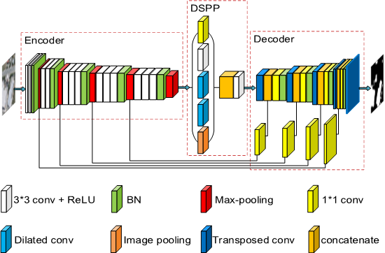
In this paper, we designed a simple but effective FCNs-based model for remote sensing images building extraction. The complete network of our proposed model is illustrated in Figure 1. As shown in the figure, we divide the model into three parts, namely encoder, DSPP and decoder.
3.1. Encoder
Currently, model training generally uses small sample slices. As the resolution of ORS images has reached the centimeter level, a large building can cover a large part of a slice. Moreover, background information plays an important role in building extraction. In order to detect large buildings, we use input images with larger size. Though large images will increase the training time, an efficient encoder is chosen to improve the efficiency of our model. We compared the floating-point operations per second (FLOPs) and training parameters of several commonly used encoders in Table 1. VGG16 has the fewest layers but the least efficiency. Xception41 seems to best meet our needs. However, due to the use of depthwise separable convolution, Xception41 needs to consume more GPU memory. Limited by the hardware resources, if we use the Xception41, we can only use a smaller batch size, which shows an adverse effect on BN layers [47]. We note that the parameters and computational cost of VGG16 are mainly concentrated in the last three convolutional layers. If we only use the first 13 layers of VGG16, we can get an encoder that meets both less parameters and low GPU memory cost requirements.
It should be noted that many researchers only use three [23,50] or four [49,51,52] downsampling layers to retain more detail features, while we keep all five pooling layers to reduce the need for hardware, mainly referring the consumption of GPU memory. As for the detail information, it is handled by the decoder. All convolutions in the encoder use 3*3 kernels and the ReLU activation function is used after each convolution. We only add a BN layer before each pooling layer rather than after each convolution layer. With this encoder, we can use larger input images and larger batch size at the same time.
3.2. DSPP
In our model, we use a dense spatial pyramid pooling (DSPP) structure after the encoder to increase the receptive field and acquire multi-scale features. The receptive field of our encoder is 212*212 which is smaller than the input image size we used. Considering that the effective receptive field was significantly smaller than the theoretical receptive field [53], we use two dilated convolution with rate = 3 (404*404) and rate = 6 (596*596) to make sure that the receptive field can cover the entire input image. However, we notice that the receptive field of DSPP is much bigger than the receptive field of encoder and the moderate features between them are ignored. Thus, we add a standard 3*3 convolution whose receptive field is 276*276. In addition, we add a 1*1 convolution to reintegrate the pooled features and an image pooling to get the importance of different feature channels. Consequently, dense and multi-scale features can be extracted by the proposed structure, and this is the first reason we call it DSPP.
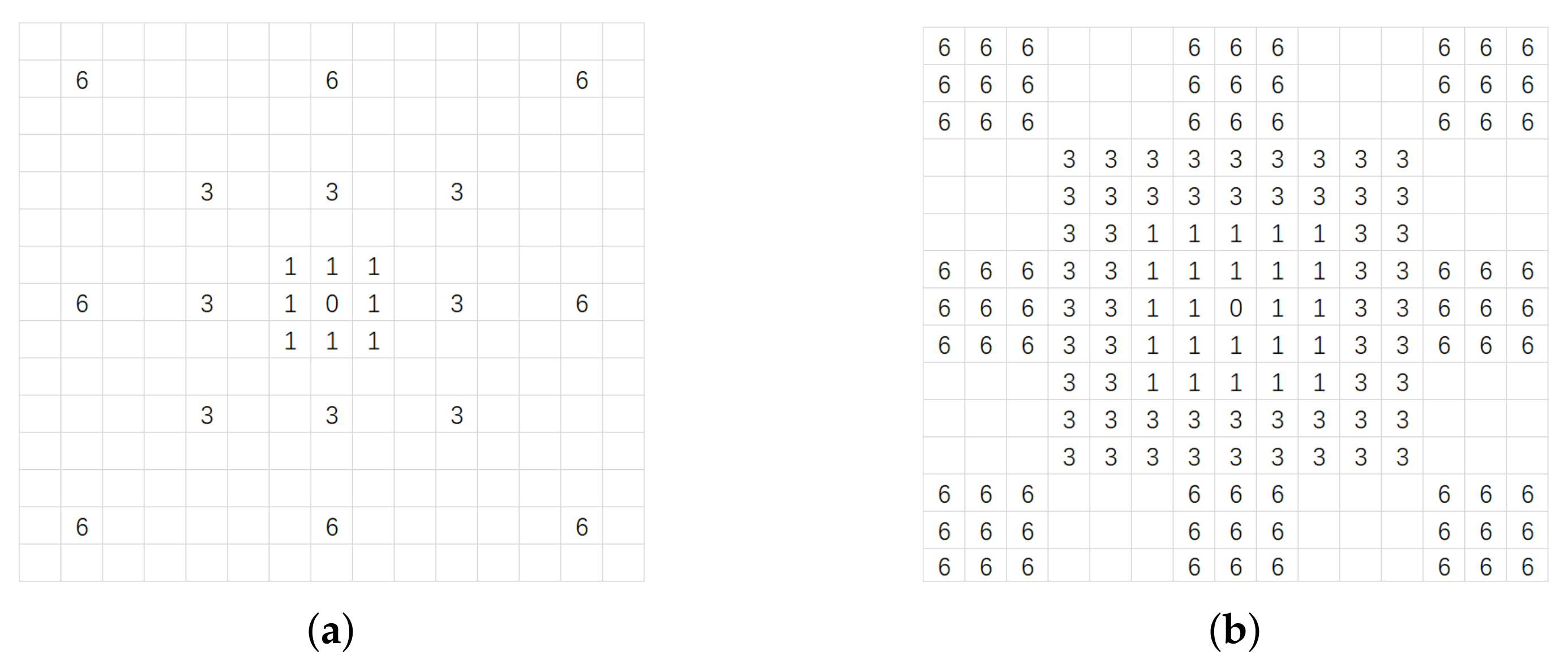
Thereafter, the concatenation of the five outputs passes a 3*3 standard convolution. Compared with the 1*1 convolution in ASPP, a 3*3 convolution can better integrate more information while reducing the feature dimension. As shown in Figure 2, the numbers represent the rates of different dilated convolutions, where 0 represents the 1*1 convolution. The position of the number indicates which feature on the input image can be used by a single pixel on the output image. Through the comparison we can see, a 1*1 convolution can only integrate very sparse features in a 15*15 pixels area, but a 3*3 convolution can nearly cover all pixels. This is another reason we call it DSPP. Finally, we add a BN layer after the 3*3 convolutional layer.
3.3. Decoder
The decoder is used to restore output resolution. We use five transposed convolutions with an upsampling factor of 2 in our decoder. In contrast to the U-Net, we do not use extra 3*3 convolutions to refine the features as shown in Figure 1, since the decoder of U-Net cannot predict accurate building boundaries. To solve this problem, we use a short connection to concatenate the outputs of the first four transposed convolution layers with the corresponding low-level layers in the encoder. However, as mentioned in paper [49], it is not the best choice to directly use the low-level features with many channels, which may outweigh the high-level semantic features and affect the final classification accuracy. Therefore, we first apply a 1*1 convolution on the low-level features before the connection to reduce the number of channels. For the best channel ratio of low-level and high-level features, we will further discuss it in Section 5. After the short connection, another 1*1 convolution is used to reintegrate features and then a BN layer is applied to accelerate model training.
3.4. Loss Function
Cross-entropy loss (CE) is the most commonly used loss function in semantic segmentation task. For binary classification, CE loss function can be described as:
where is the ground truth label and is the prediction result. For notational convenience, here we define the probability as:
Then, we can rewrite the loss function in (3) as:
Focal loss (FL) [54] is proposed to address extreme imbalances between foreground and background classes in dense object detection. Now, it is also often used to deal with category imbalances in semantic segmentation. Focal loss is improved from CE loss. To address class imbalance, an intuitive idea is to use weighting coefficients. The modified CE loss function can be expressed as:
is the weighting factor for the two classes, which is defined analogously to .
Based on this, FL adds a modulating factor to further reduce the loss of the easy classification category. is a tunable focusing parameter. FL function can be described as:
As , the factor , i.e., samples that have been correctly classified tend to show a reduced impact on the model training. Conversely, samples that are difficult to classify will determine the subsequent model training. Through the focusing factor , the rate at which easy samples are downweighted can be smoothly adjusted. FL is equivalent to CE when .
In our task, the error ground truth labels instead of the category imbalance are the most serious impact that constrains the effectiveness of the model training. We can regard the error labels as hard examples in FL function, and eliminate the influence of error labels by constraining its weight in the later stages of training. Therefore, our final loss function is:
is the weighting factor to control the weight of FL in total loss. The larger the , the smaller the impact of the difficult (error) sample on the model training. By using the FL in reverse, we can reduce the impact of error labels in CE. Lin et al. [54] pointed out the best choice was and and worked nearly as well. In our task, two typical error labels, the missing of buildings and the error classification of buildings, are considered. We think these two kinds of error labels should be treated equally, and thus we set . As for the , we follow the setting in [54] as (Appendix A).
4. Experimental Results
In this section, we first present detailed dataset description, implementation settings, evaluation metrics and comparative methods. Then, extensive experiments were performed to evaluate the performance of the proposed EU-Net.
4.1. Dataset Description
In this paper, we evaluate the proposed EU-Net on three publicly available building datasets for semantic labeling. The metrics of subsequent experiments are evaluated on the test sets of three datasets.
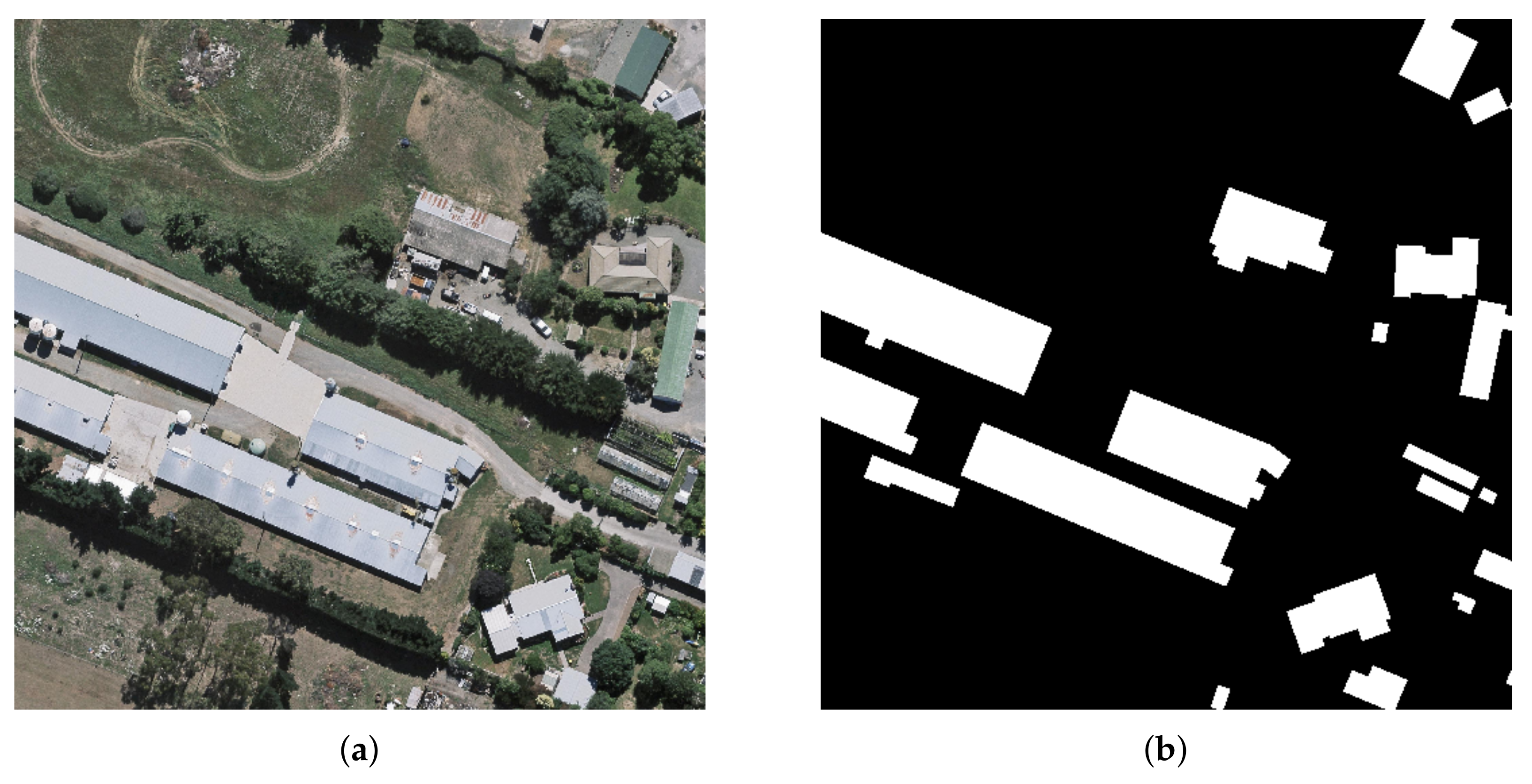
WHU Building Dataset: This dataset is proposed in [5] and includes both aerial and satellite images. In this paper, we only use the aerial imagery dataset (0.3 m ground resolution) which has higher label accuracy. Therefore, we use this dataset to evaluate the accuracy of building extraction. The aerial dataset contains 8189 tiles with 512*512 pixels. Paper [5] divided the samples into three parts: a training set (4736 tiles with 130,500 buildings), a validation set (1036 tiles with 14,500 buildings) and a test set (2416 tiles with 42,000 buildings). An example is shown in Figure 3.
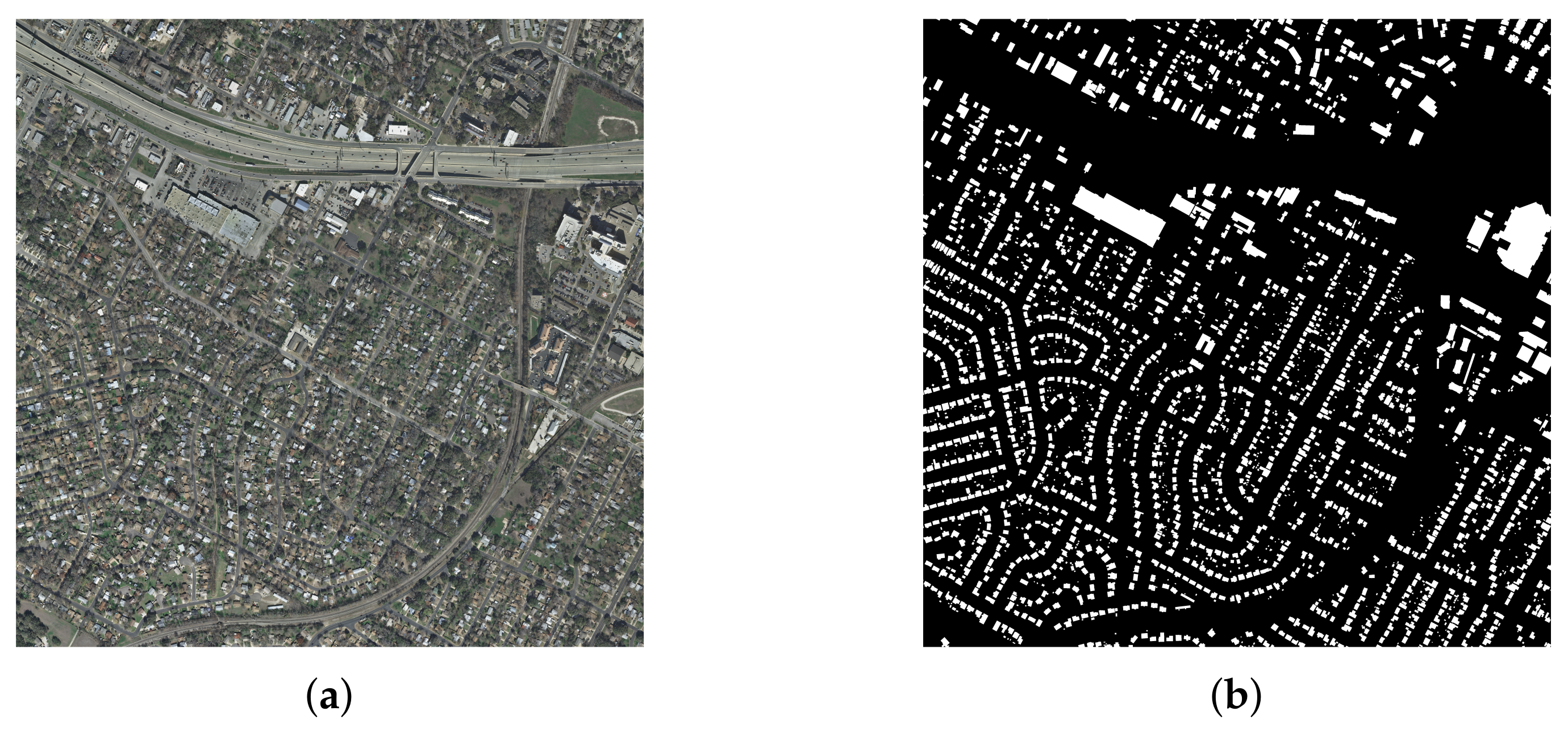
Massachusetts Building Dataset: This dataset is proposed in [6]. Unlike the WHU dataset, the ground resolution of this dataset is 1m, which is relatively low. The label accuracy of this dataset is also lower than the WHU dataset. Thus, we use this dataset to evaluate the ability to handle fuzzy images. There are 151 images with 1500*1500 pixels and paper [6] divided them into three parts: a training set of 137 images, a validation set of 4 images and a test set of 10 images. An example is shown in Figure 4.
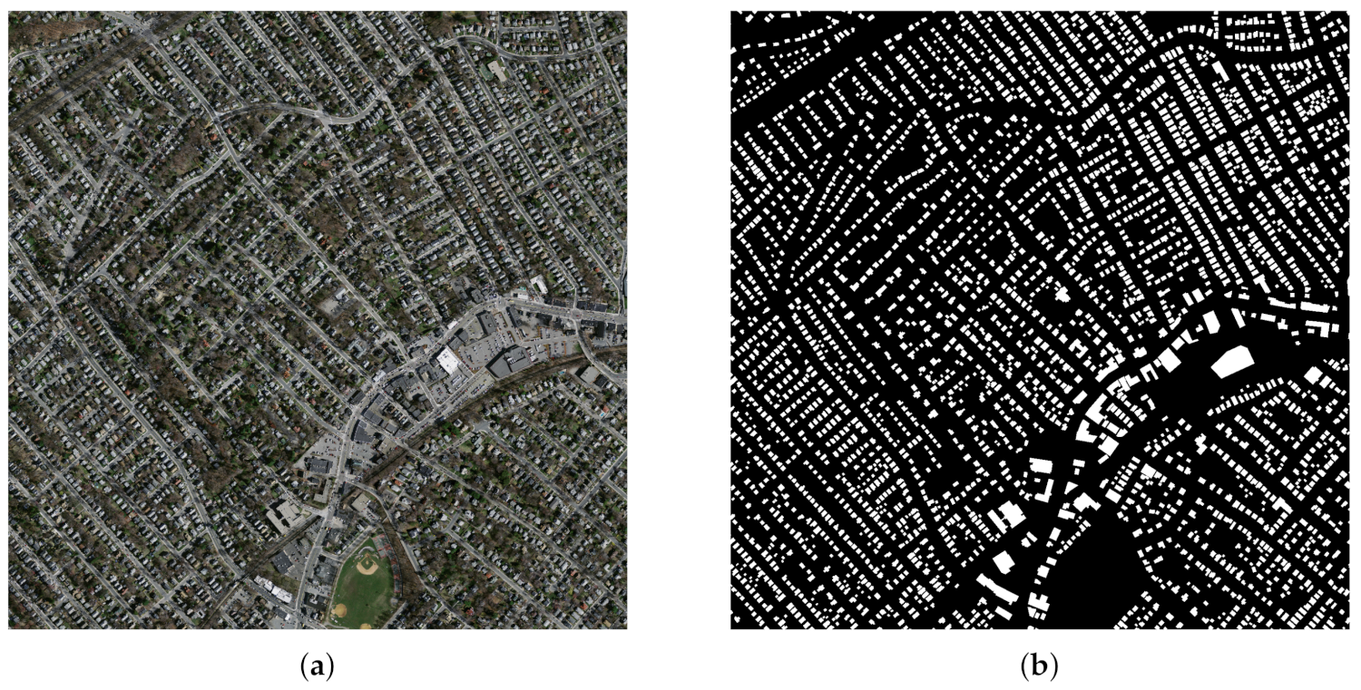
Inria Aerial Image Labeling Dataset: This dataset is proposed in [7] and includes 180 images with public labels and 180 images without public labels. For quantitative analysis, we only use the former in this paper. There are five dissimilar urban settlements (Austin, Chicago, Kitsap County, Western Tyrol and Vienna) with 36 images respectively, ranging from densely populated areas to alpine towns. Since the label accuracy of this dataset is lower than the first dataset, we use this dataset to evaluate the generalization ability of the model. The ground resolution of this dataset is also 0.3 m and image size is 5000*5000 pixels. The first five images of each city are set as test images. An example is shown in Figure 5.
4.2. Implementation Settings
Due to hardware limitations, raw images are too large to be directly used for training. In this paper, the raw images are cropped into 512*512 patches in preprocessing with no overlap. The WHU dataset has 4736 512*512 patches, the Massachusetts dataset has 1065 512*512 patches, and the Inria dataset has 15,500 512*512 patches. Then, in each iteration, a batch is clipped to 256*256 pixels using the same random cropping to further increase the diversity of the training samples. Except for random cropping, we do not use other data augmentation tricks such as rotation and flip.
We implemented our EU-Net model based on the Keras API in TensorFlow framework. In the experiments, we did not use any pre-training parameters. The convolution kernels were initialized with Glorot uniform initializer [55] and the biases were initialized to 0. Our proposed network was trained from scratch using SGD optimizer with batch size 64, momentum 0.9. Unlike most literature, we did not use any learning rate adjustment strategies. For the WHU dataset and the Inria dataset, the learning rate was set to 0.2. And for the Massachusetts dataset, the learning rate was set to 0.5. As for the in (6), we set 0 for the WHU dataset, and 2 for the Massachusetts dataset and the Inira dataset. This was because the WHU dataset had a high-precision label and therefore did not require the FL. The model was trained using two NVIDIA GeForce GTX 1080Ti and tested with one. We trained EU-Net 300 epochs with WHU dataset, 2000 epochs with Massachusetts dataset, and 400 epochs with Inria dataset.
4.3. Evaluation Metrics
To assess the quantitative performance, four benchmark metrics are used, i.e., recall (Rec), precision (Pre), F1 score (F1) and intersection over union (IoU). These four metrics are defined as:
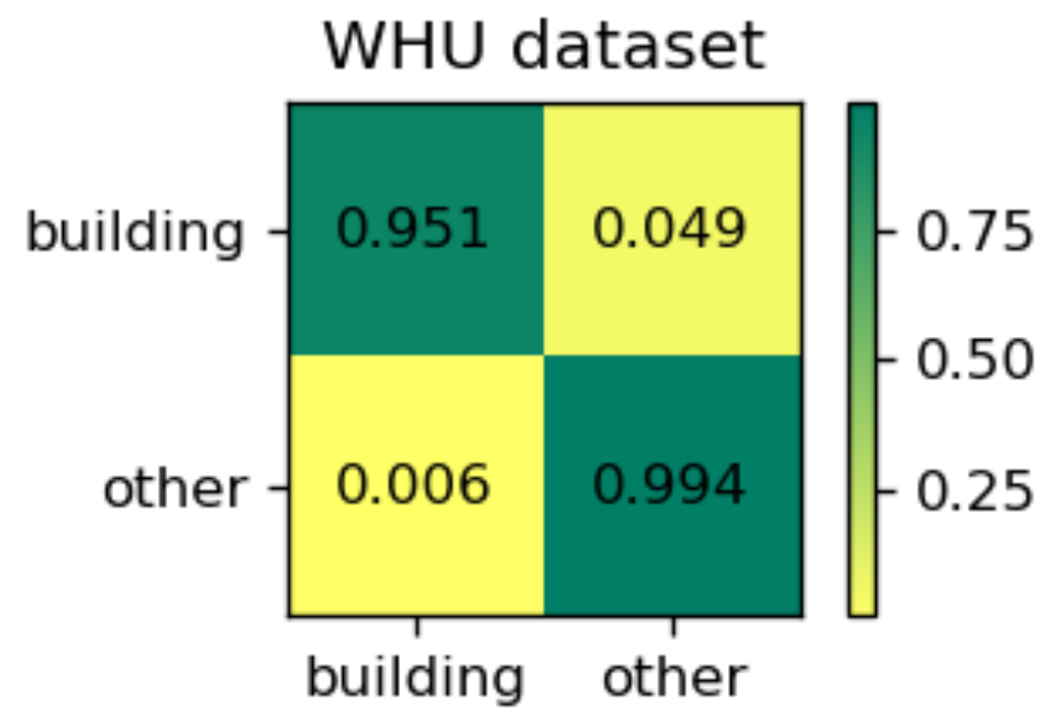
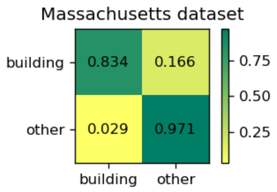
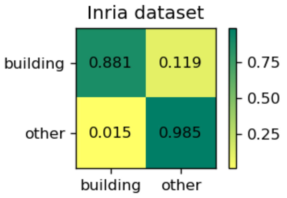
where TP, FP and FN are the number of true positives, false positives and false negatives, respectively. In addition, we will give the normalized confusion matrix, following [56,57]. The form of normalized confusion matrix is shown in Figure 6. The indexes in the row denote the rates of the pixels that are classified as each class from the class.
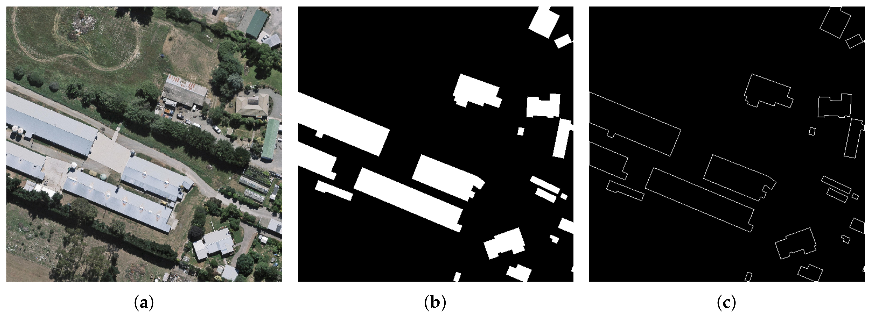
As we all know, every building has a clear boundary, no matter how the shape of the building changes. Therefore, in addition to using the original mask labels, we also create contour labels to evaluate the model. The criterion for judging whether a building pixel belongs to the contour is based on whether there are background pixels among its four adjacent pixels. If the judgment is true, then the pixel is a contour pixel, and vice versa. An example of the contour label in WHU dataset is shown in Figure 7.
The four metrics based on mask labels and contour labels are both presented in the subsequent experiments.
In addition to extraction accuracy, the efficiency of the model is also our focus. Considering that the size of the original image in the WHU dataset is only 512*512 pixels, we use the number of images processed per second by the model as a metric. As for the other two datasets, we use the time processing an image as the metric.
4.4. Comparing Methods
To demonstrate its superior performance, the proposed EU-Net is compared with the state-of-the-art methods on each dataset. In this subsection, we will give a brief introduction of the best performing model on each dataset. In addition, we use the results of DeepLabv3+ and FastFCN as the benchmarks for all three datasets.
SRI-Net: Liu et al. [22] proposed SRI-Net for building detection, which was tested on the WHU dataset and the Inria dataset. According to our research, it achieved the best performance on the WHU dataset. We reproduced the SRI-Net with the Keras API and retrained it on the WHU dataset. We followed the training settings in [22]: an Adam optimizer was initialized with a learning rate of 1 × 10, the learning rate was decayed at a rate of 0.9 per epoch, L2 regularization was introduced with a weight decay of 0.0001. Cross-entropy was used as loss function. We trained SRI-Net 300 epochs on WHU dataset.
JointNet: Zhang et al. [24] proposed JointNet for building detection, which was tested on the Massachusetts dataset. According to our research, it achieved the best performance on this dataset. We reproduced the JointNet with the Keras API and retrained it on the Massachusetts dataset. We followed the training settings in [24]: an Adam optimizer was initialized with a learning rate of 1 × 10, and focal loss was used as loss function. We trained JointNet 400 epochs on Massachusetts dataset.
Web-Net: Zhang et al. [38] proposed a nested encoder-decoder deep network for building extraction, named Web-Net. To balance the local cues and the structural consistency, the Web-Net used the Ultra-Hierarchical Sampling (UHS) blocks to extract and fuse the inter-level features. According to our research, it achieved the best performance on the Inria dataset. In order to achieve the best result, Web-Net had to use the pretrained parameters from ImageNet.
FastFCN: The FastFCN model was proposed by Wu et al. [20] and achieved the state-of-the-art results on the ADE20K dataset and the PASCAL Context dataset. We reproduced the FastFCN with the Keras API. We trained FastFCN 300 epochs on WHU dataset, 1600 epochs on Massachusetts dataset, and 350 epochs on Inria dataset. FastFCN was trained with SGD, of which the momentum was set to 0.9 and the weight decay was set to 1 × 10. We set the learning rate to 0.1 and reduced it following the ‘poly’ strategy. Loss function was kept same with EU-Net.
DeepLabv3+: The DeepLab networks were proposed by Chen et al. and have been improved several times, including v1 [21], v2 [58], v3 [59], and v3+ [49]. The DeepLabv3+ achieved the state-of-the-art results on the Cityscapes dataset and the PASCAL VOC 2012 dataset. We reproduced the DeepLabv3+ with the Keras API. We trained DeepLabv3+ 300 epochs on WHU dataset, 1600 epochs on Massachusetts dataset, and 400 epochs on Inria dataset. DeepLabv3+ was trained with SGD, of which the momentum was set to 0.9 and the weight decay was set to 1 × 10. We set the learning rate to 0.01 for WHU dataset, 0.5 for Massachusetts dataset, and 0.01 for Inria dataset. We also reduced the learning rate following the ’poly’ strategy. Loss function was kept same with EU-Net.
4.5. Comparison with Deep Models
4.5.1. WHU Dataset
Table 2 gives the quantitative evaluation indexes of different models on the test images of the WHU dataset. Our proposed EU-Net outperforms SRI-Net, FastFCN, and DeepLabv3 on all the four metrics, except for the precision of SRI-Net. However, the precision of our EU-Net is only 0.23% lower than that of SRI-Net, and our EU-Net makes a better balance between recall and precision, as can be intuitively seen from the F1. The mask IoU metrics are all higher than 85% and our EU-Net even exceeds 90%. This is because the WHU dataset is of higher quality and is easier to distinguish than the other two datasets [22]. Compared with the result of SRI-Net in [22], our EU-Net improved the mask IoU by 1.47%. Moreover, our model can process 16.78 images per second, while SRI-Net can only process 8.51 images per second. In other words, our model efficiency is approximately twice that of the latter. The FastFCN and the DeepLabv3+ are also much slower than our model. As a reference, we also presented the normalized confusion matrix for EU-Net in Figure 8.
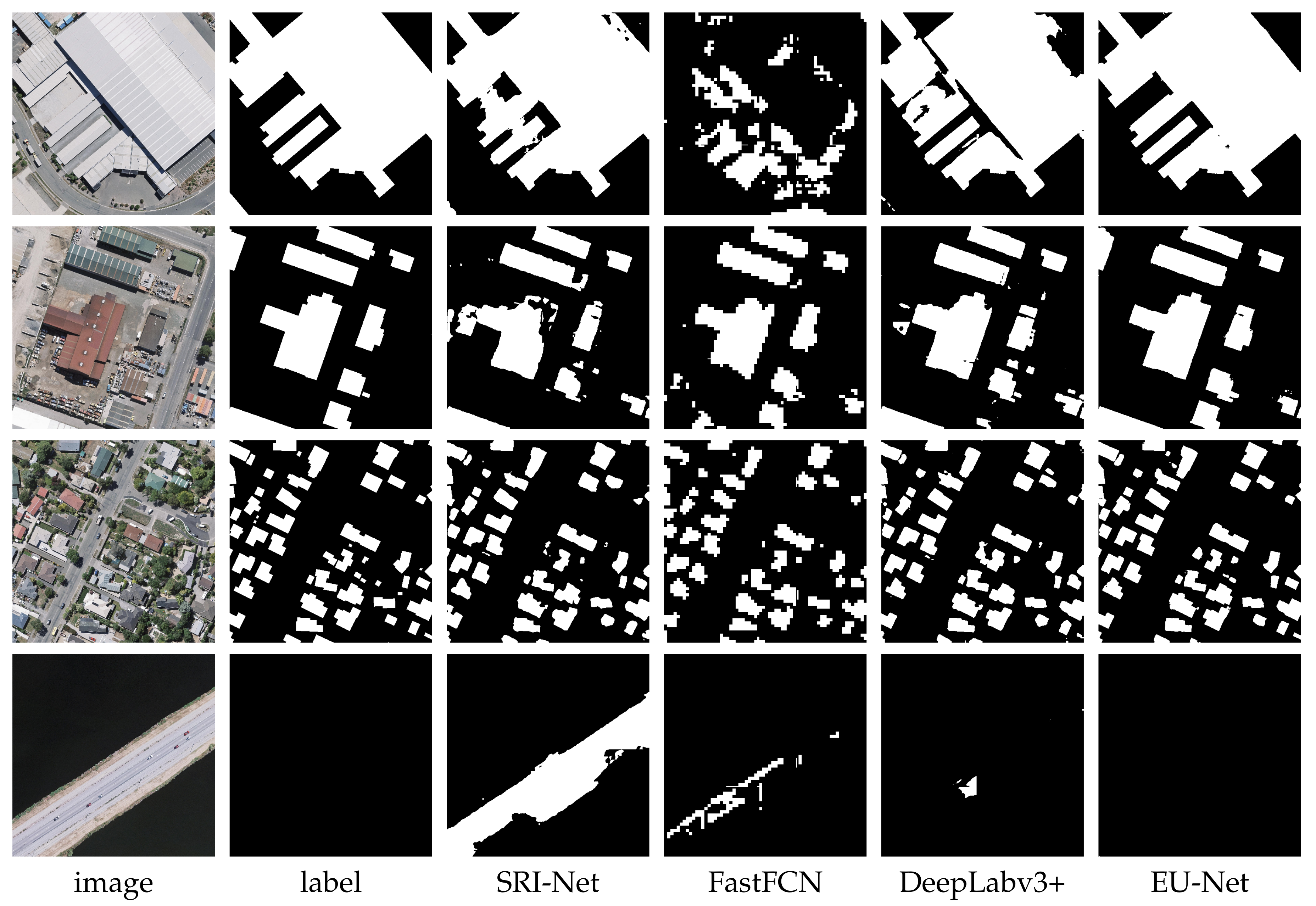
Figure 9 shows the visual performance of four different scenarios. The first scenario is an example of an oversized building. The result of FastFCN was very terrible where the oversized building was almost undetected. SRI-Net and DeepLabv3+ misclassified the cement floor in the lower middle area into buildings, while our EU-Net successfully avoided this error. The second scenario is sparsely distributed medium-sized buildings. Only our EU-Net successfully detected the building in the upper left corner and all four models misclassified the containers in the lower right corner into buildings. The third scenario is densely distributed small-sized buildings. All four models missed several buildings of very small size. The fourth scenario is a negative sample. Only our EU-Net gave the right prediction and the other three models had more or less misclassifications. In summary, our EU-Net gives the best results both on the integrity of building shapes and the accuracy of building contours.
4.5.2. Massachusetts Dataset
In this dataset, we predicted the test images in blocks of 512*512 pixels, with a sliding stride of 256 pixels. Table 3 gives the quantitative evaluation indexes and time costs of processing one image for different models. It is clear that our proposed EU-Net outperforms JointNet, FastFCN, and DeepLabv3+. Compared with the results of the WHU dataset, all metrics are much lower for the four models. There are two reasons for the results. First, the scenes of the Massachusetts dataset are more complicated. Especially the shadows of high buildings bring great difficulties to the classification. Second, the Massachusetts dataset has a lower resolution and label quality. As shown in Table 3, recall metrics for all models are much lower than the precision metrics and our model has the smallest gap between the two metrics. Compared with the report result of JointNet in [24], our EU-Net improved the IoU by 1.94%. In terms of processing efficiency, the FastFCN is almost the same as the DeepLabv3+, and the time to process one image is nearly twice that of our model. The most time-consuming JointNet takes more than three times as much as our model. As a reference, we also presented the normalized confusion matrix for EU-Net in Figure 10.
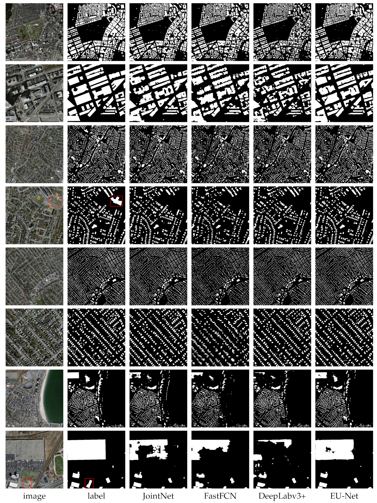
Figure 11 shows the visual performance of four different scenarios. The odd rows are original images and the even rows are the regions of interest selected by red boxes in the original images. The first scenario showed the impact of high-rise shadows on the accuracy of building extraction. It could be seen that the buildings predicted by four models were all incomplete and the integrity of DeepLabv3+ was the worst. Although the integrity of FastFCN was better than DeepLabv3+, there was a significant sawtooth effect on the building contours. Our EU-Net gave the most complete and accurate building extraction results. The main problem was that the shadows in the middle of the buildings cannot be accurately classified. As mentioned before, there exist obvious wrong labels in Massachusetts dataset. An example of error labels is shown in the 4th and 8th row of Figure 11, where the ground truth presents a wrong label on the grassland area. The last two scenarios were used to show the performance of four models for detecting buildings of different sizes. For small and medium-sized buildings, JointNet, DeepLabv3+ and EU-Net had similar performance. Meanwhile, for oversized buildings, only our EU-Net gave a relatively complete prediction.
4.5.3. Inria Dataset
The test image size is the same as the Massachusetts dataset. Table 4 gives the quantitative evaluation indexes and time costs of processing one image for different models. Similar conclusions can be drawn from Table 4. The results on the Inria dataset are also worse than the WHU dataset, but better than the Massachusetts dataset. The latter is because the resolution of the Inria dataset is higher than the resolution of the Massachusetts dataset. Compared with the WHU dataset, the Inria dataset has a lower quality where some obvious error labels can be found in the ground truth. Moreover, the scenes of the Inria dataset are more complicated, as there are five different cities in the dataset. These factors cause the results on the Inria dataset to be worse than the WHU dataset. Compared with the result of Web-Net reported in [38], our EU-Net improved the mask IoU by 0.4%. According to paper [38], the Web-Net takes 56.5 s to process one image, while the EU-Net only needs 14.79 s, i.e., our model has improved the efficiency four times compared with the Web-Net. As a reference, we also presented the normalized confusion matrix for EU-Net in Figure 12.
We also test the performance of EU-Net on five cities respectively, showed in Table 5. Compared with Web-Net, the proposed EU-Net gained better performance on Austin, Chicago, and Vienna. But for Kitsap and Tyrol-w, Web-Net performed better. In general, the overall performance of the proposed EU-Net is slightly better than Web-Net.
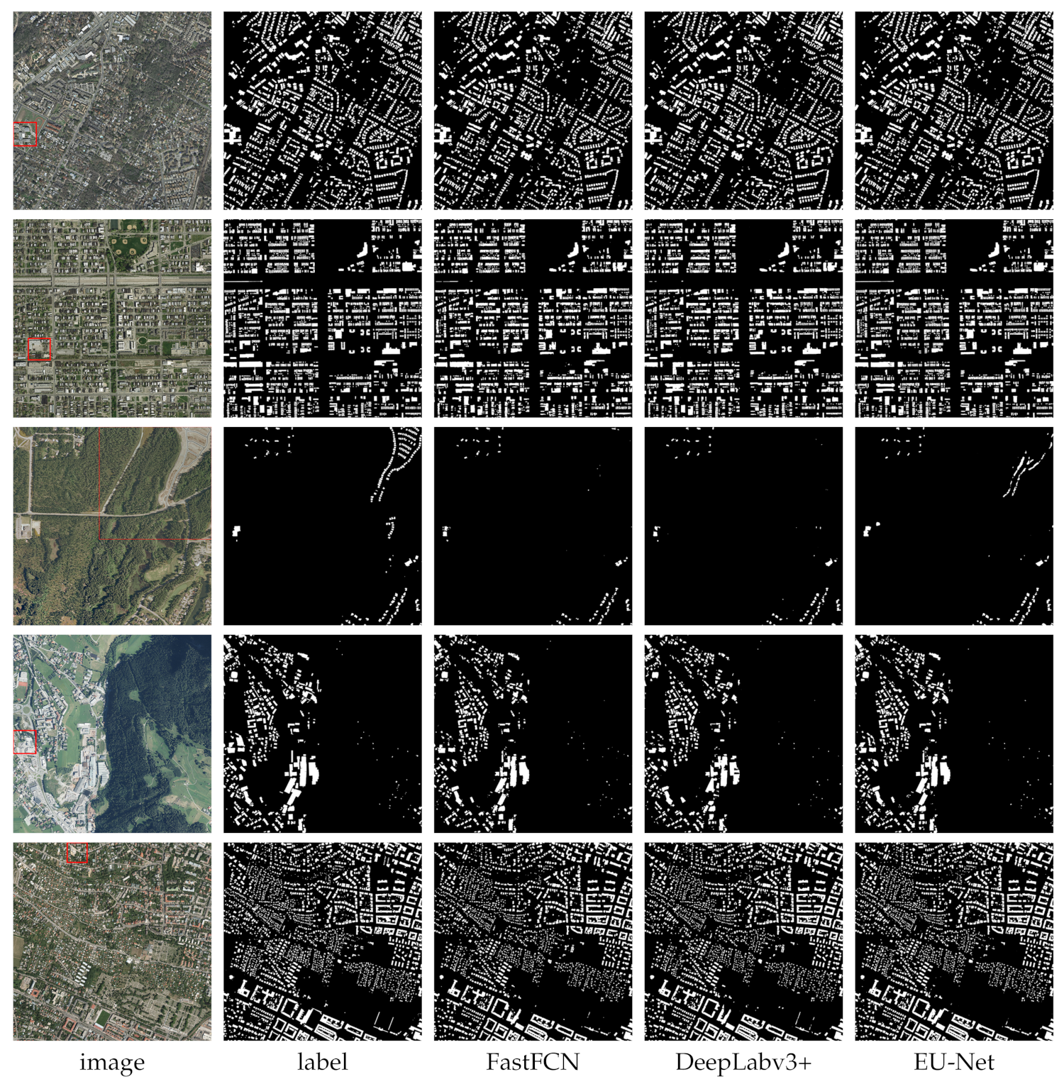
We selected a representative image from each of the five cities, as shown in Figure 13. The buildings in Kitsap County (the third row in Figure 13) are randomly scattered throughout the image and the buildings in Western Tyrol (the fourth row in Figure 13) are concentrated in parts of the image. The buildings of the other three cities are densely distributed throughout the images. Among them, the buildings in Chicago (the second row in Figure 13) are neatly distributed, while the buildings in Austin (the first row in Figure 13) and Vienna (the last row in Figure 13) are irregular. Compared with Austin, the building size varies drastically in Vienna.
Roughly speaking, the three model predictions are visually similar. In order to compare the details, we enlarged the red boxes in Figure 13, shown in Figure 14. From top to bottom are Austin, Chicago, Kitsap, Tyrol and Vienna. For the large buildings in Austin, the predictions of FastFCN and our model were more complete than DeepLabv3+, and the contour accuracy of DeepLabv3+ and our model was better than that of FastFCN. Moreover, there were some misclassifications of small-size buildings in the predictions of FastFCN and DeepLabv3+. For the Chicago, there are many neatly arranged buildings. In the prediction of FastFCN, the adjacent buildings were treated as a whole. The prediction of DeepLabv3+ was slightly better, and only EU-Net successfully distinguished these buildings. In addition, the selected areas in Chicago showed some error labels. Although all three models gave correct predictions for these areas, they gave some false alarms as shown in the yellow rectangles. Moreover, the large building in the prediction of DeepLabv3+ obviously missed the right piece. As for the Kitsap, all buildings in the selected area were error labels. Our EU-Net showed a bad performance while the predictions of DeepLabv3+ and FastFCN only had a few noises in the selected area. We ascribed the bad performance to the simple encoder of EU-Net. Compared with the other four cities, there were much fewer buildings in Kitsap, and thus it was difficult for models to learn enough effective features to correctly extract the buildings in Kitsap, especially for our simple encoder. This conclusion can be also drawn from the quantitative indexes on Kitsap among the five cities. Because there were few buildings in the Kitsap, the error labels had a great influence on the evaluation metrics, leading to abnormally low metrics in this area. If we ignored these obviously error labels, the IoU metrics for EU-Net, DeepLabv3+ and FastFCN could be improved by 4.91%, 7.83% and 7.50%, which were obvious improvements. There are four large buildings in Tyrol. The prediction results of FastFCN and DeepLabv3+ missed two of them while the EU-Net extracted four buildings. As for the enlarged areas in Vienna, the buildings in yellow box were under construction. It is clear that the FastFCN and DeepLabv3+ both failed to extract the two buildings, and the proposed EU-Net successfully detected one of them.
5. Discussion
5.1. Channel Ratio in Short Connection
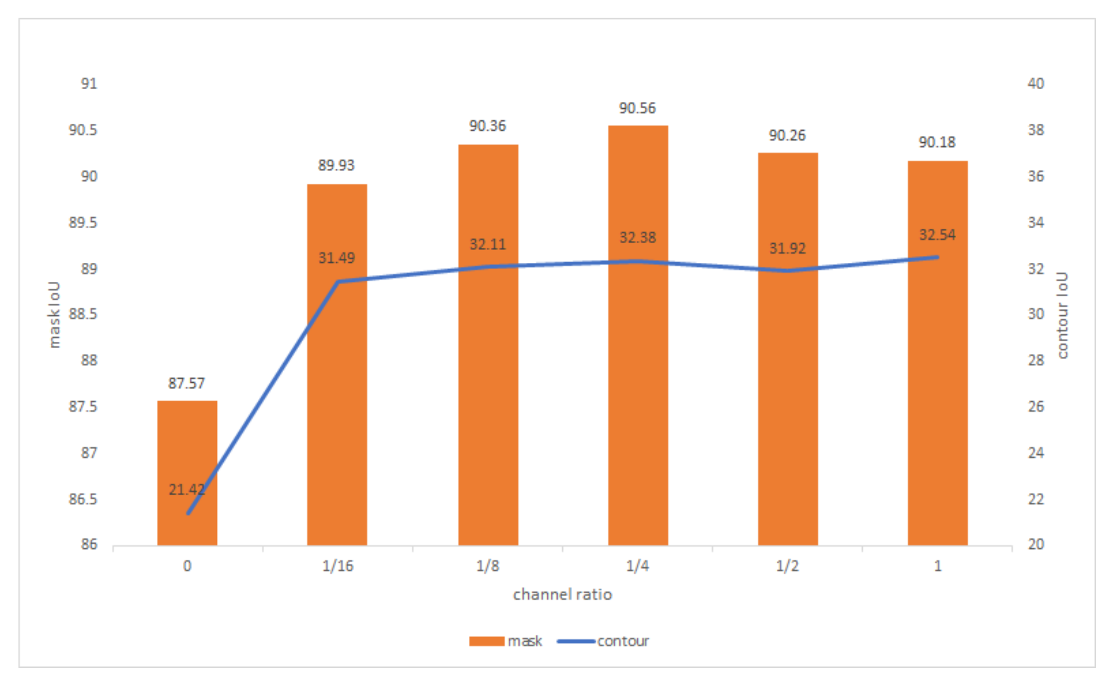
Unlike natural objects, buildings are a type of artificial objects with clear boundaries. Therefore, we hope to obtain more accurate building contours when improving the overall classification accuracy. As we know, shallow focal features have more detailed information, while rich semantic information in deep global features is more conducive to overall classification. Consequently, we want to choose a best channel ratio between shallow features and deep features in the short connection. A comparative experiment of the channel ratios versus IoU is presented in Figure 15, where 0 means no short connection is used, and 1 means the shallow features have the same channels with deep features. Obviously, the result is much worse without using short connections. Basically, the contour IoU increases as the channel ratio increases and the mask IoU increases first and then decreases. When the ratio is less than 1/4, the addition of shallow features can provide more accurate position information for the semantic features, thereby improving the segmentation accuracy. When the ratio exceeds 1/4, the model will pay too much attention to detail accuracy and ignore the semantic integrity. When ratio is 1/4, the mask IoU achieves the maximum value and therefore the channel ratio is set as 1/4.
5.2. Larger Sample Size or Larger Batch Size
Training sample size has a strong influence on the training model since models can potentially capture more fine-grained patterns with higher resolution samples [61]. In the case of limited hardware resources, the batch size must be reduced to increase the sample size. However, as mentioned before, BN is sensitive to input batch size. Considering the performance of BN layers, the batch size should not be too small. So, which one is more important for building extraction, the larger sample size or the larger batch size?
To make full use of GPU memory, we set up three sets of comparison experiments for (sample size, batch size), which are (256*256, 64), (354*354, 32) and (512*512, 16). Table 6 lists the IoU metrics of each set on the three datasets. We can see that increasing the sample size and reducing the batch size make the mask IoU metrics worse on three datasets, i.e., for building extraction, a larger batch size is more important than a larger sample size. In addition, the metric gaps on the Inria dataset were the smallest. For the other two datasets, the results of (512*512, 16) had a significant drop. We think this is because there are no sufficient training samples for the first two datasets when sample size is 512*512. Specifically, the WHU dataset has 4737 samples and the Massachusetts dataset only has 1065 samples. Conversely, for the Inria dataset with sufficient samples, the contour IoU metric of (512*512, 16) is even better than that of (354*354, 32). Overall, the best parameter setting is (256*256, 64).
To further verify the impact of batch size and sample size on model training, we used the Inria dataset to supplement three sets of contrast experiments (224*224, 64), (256*256, 32) and (256*256, 16). When training model with the latter two sets of parameters, only one NVIDIA GeForce GTX 1080Ti was used. The IoU metrics are list in Table 7. As expected, compared with the results in Table 6, the IoU continues to decrease as the batch size decrease when the sample size is fixed. And the IoU increases as the sample size increases when batch size keeps same. Consequently, we think that our EU-Net will work better when trained with large sample size and large batch size at the same time.
5.3. DSPP
In this subsection, we will verify the effect of DSPP block by ablation experiment. Training sample size and batch size are set to 256*256 and 64. The EU-Net model without DSPP block is denoted as EU-Net-simple. We tested the EU-Net-simple with three datasets and compared them with the previous experiment results. The IoU metrics are showed in Table 8, and we can see that the IoU metrics have improved on all three datasets by using the DSPP. The minimum increase is 0.35% on the WHU dataset and the maximum increase is 1.76% on the Inria dataset.
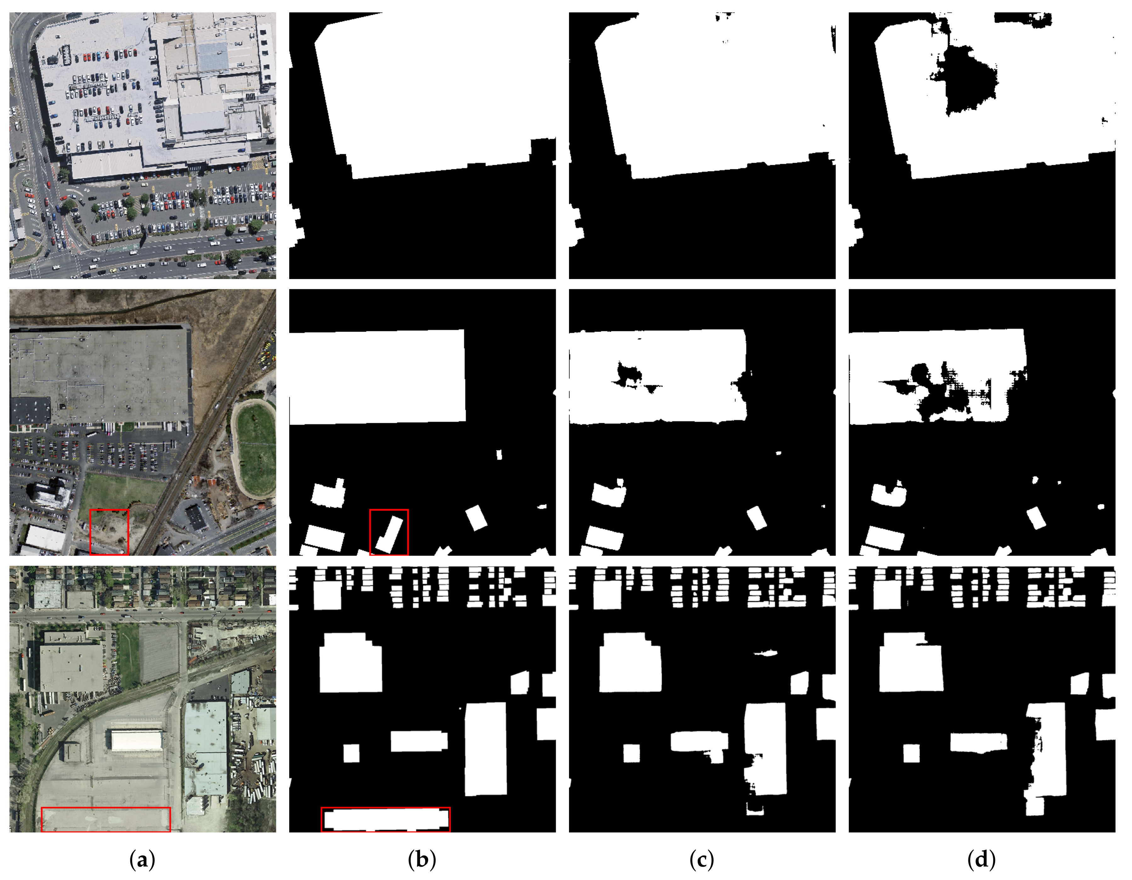
We propose to use DSPP to acquire multi-scale features, which can improve the extraction accuracy of buildings of different sizes, especially the medium-sized and oversized buildings. For a clearer visualization, we chose an obvious area from each dataset. The selected areas are shown in Figure 16. For the WHU block, part of the roof parking was misclassified in the result of EU-Net-simple. For the Massachusetts block with multi-scale buildings, the extraction accuracy of EU-Net was higher for all buildings of different sizes. As for the Inria block, the results of the small-sized buildings had no significant difference. EU-Net clearly performed better on the large building extractions. All the above results demonstrate that DSPP does play its intended role. The red box selected areas in the Massachusetts block and the Inria block are error ground truth labels, and both models gave the right predictions.
Moreover, adding DSPP block does not significantly reduce the efficiency of the model. We compare the time of processing one image in the Inria dataset. The EU-Net-simple took 13.95 s, and the EU-Net took 14.79 s. After adding DSPP block, consuming time to process a 5000*5000-pixel image only increased 0.84 s. This time increase is worthwhile compared to the increase in metrics.
5.4. Loss Function
The error labels can hinder model training. To overcome this problem, we introduced FL in reverse to reduce the gradient generated by the error labels. We also verified the performance of FL through comparative experiments. We set to remove the FL from loss function and performed the EU-Net on the Massachusetts dataset and the Inria dataset. Training sample size and batch size were still set to 256*256 and 64. The IoU metrics are listed in Table 9. The mask IoU has been improved on the Massachusetts dataset by 1.1% and improved on the Inria dataset by 0.05%. It turns out that negative FL does work. In addition, we can see that even without using FL, the results of our EU-Net are better than the state-of-the-art results on these two datasets.
Table 9 proved that negative FL does work. To analyze the influence of the FL weight, we changed to 1 and 3, and retrained EU-Net on Massachusetts dataset. The IoU metrics are listed in Table 10. For both mask IoU and contour IoU, the maximums were obtained when was 2. Therefore, we set to 2 when training the model on Massachusetts dataset and Inria dataset.
5.5. Learning Rate and Epoch
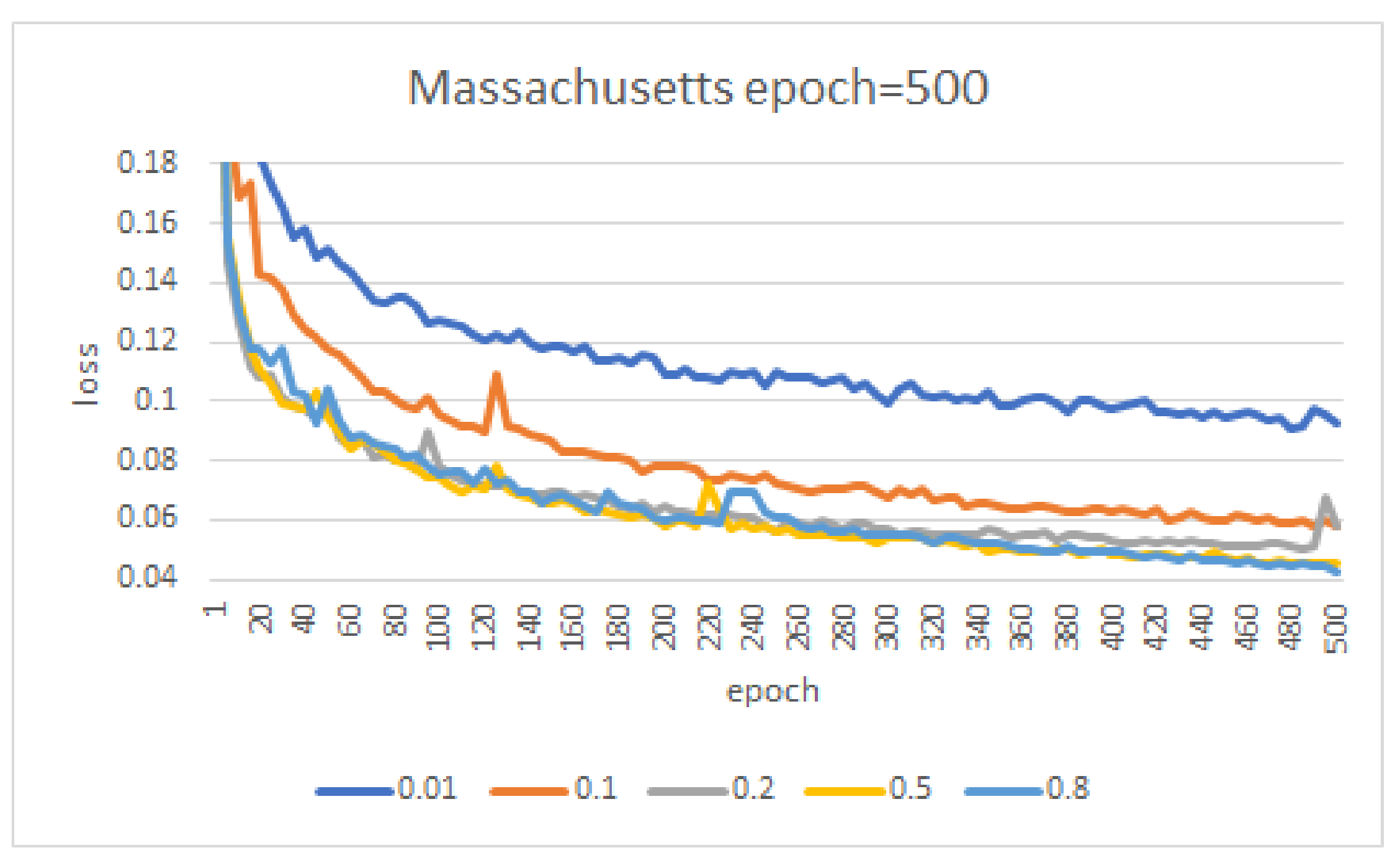
The learning rate and number of epochs can greatly affect the model performance. In order to obtain the optimal hyperparameters, we conducted some comparative experiments. As we know, the learning rate affects the convergence speed of the model, and increasing the learning rate in a certain range can speed up the network convergence. Therefore, we used different learning rates and fixed the number of epochs to test the convergence speed of the network. Taking the Massachusetts dataset as an example, we started with the learning rate of 0.01 and then increased to 0.1, 0.2, 0.5 and 0.8. For different learning rates, we fixed the number of epochs to 500. As shown in Figure 17, the convergence speed continues to increase until the learning rate reaches 0.5. While continuing to increase to 0.8, the convergence speed has no obvious increasing. Consequently, we use learning rate of 0.5 to train EU-Net on Massachusetts dataset.
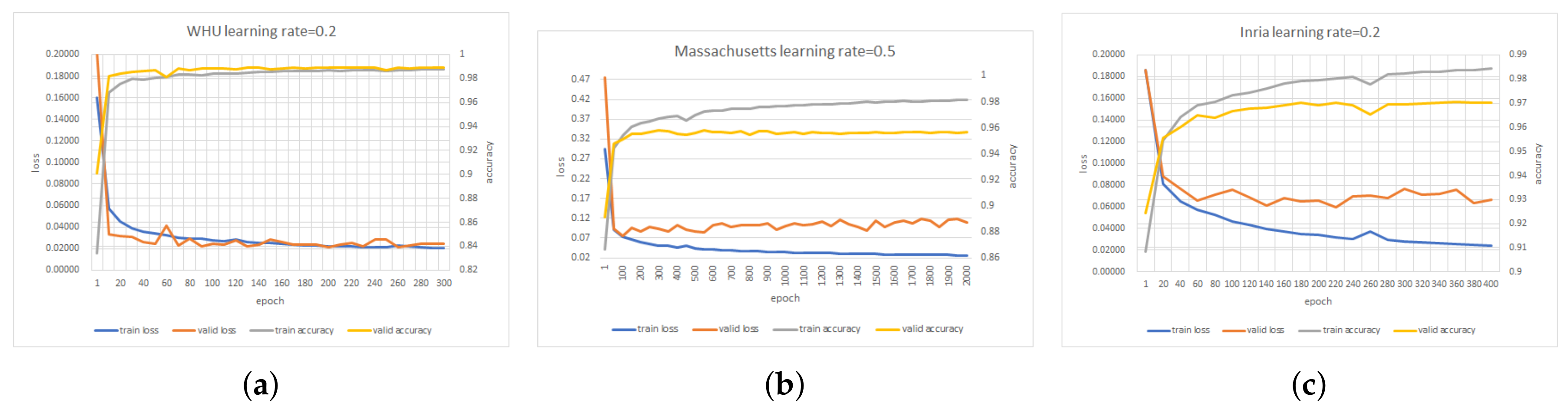
After determining the appropriate learning rate, we trained our model with more epochs. As shown in Figure 18a, the valid_accuracy curve tends to be flat when the number of epochs increases to 300, and the valid_loss curve has no obvious upward trend, which means that model has no overfitting. Consequently, 300 epochs are sufficient to train EU-Net on WHU dataset. We can see from Figure 18b,c that although the valid_accuracy curves have not decreased, the valid_loss curves have begun to increase. In other words, continuing to train the model may lead to overfitting. Therefore, 2000 epochs and 400 epochs are sufficient to train EU-Net on Massachusetts dataset and Inria dataset.
6. Conclusions
In this paper, we proposed an effective FCN-based neural network model for building extraction from aerial remote sensing images. The proposed network consists of three parts: encoder, DSPP block and decoder. In order to save GPU memory cost, we chose the first 13 layers in VGG16 as our encoder. Then, we can train our model with large batch size and learning rate to improve training efficiency. The DSPP block was proposed to enlarge the receptive field and extract dense multi-scales features. In the decoder, by adjusting the channel ratio of the deep features and the shallow features, we can achieve higher building contour accuracy as much as possible while improving the semantic segmentation accuracy.
The experiments were conducted on three datasets. Experimental results show that the DSPP block can improve the extraction accuracy of multi-size buildings. The impact of error labels in training samples could be successfully suppressed by using the focal loss in reverse. Without any post-processing, our model refreshed the state-of-the-art performance on the three datasets simultaneously.
Although our model has achieved satisfactory results, the building boundary accuracy is still very low. In future studies, we will try to modify the loss function or adjust the network structure to improve the extraction accuracy of the building contours.
Author Contributions
Conceptualization, W.K.; Methodology, W.K.; Resources, F.W.; Supervision, F.W. and H.Y.; Validation, Y.X.; Writing—original draft, W.K.; Writing—review & editing, Y.X., F.W. and H.Y.
Funding
This research was funded by the From 0 to 1 Original Innovative Project of the Chinese Academy of Sciences Frontier Science Research Program under Grant ZDBS-LY-JSC036, and the National Natural Science Foundation of China under Grant 61901439.
Acknowledgments
The authors would like to thank the anonymous reviewers for their constructive comments and suggestions.
Conflicts of Interest
The authors declare no conflict of interest.
Appendix A. Derivatives
We use y = 1 to specify the building label and y = −1 to specify the others. A pixel in output map has two predictions, which we denote as x for label y = 1 and for label y = −1. Before calculating the loss, we use SoftMax to calculate the probability p that a pixel belongs to building. p can define as:
Derivative for p regarding x is:
Then, we use to specify the pixel belongs to different classes. can defined as:
This is compatible with Equation (2). According to the chain rule, derivative for regarding x is:
According to Equations (3) and (5), we can get the derivatives for CE and FL regarding are:
According to the chain rule, derivatives for CE and FL regarding x are:
According the definition of loss function in Equation (6), derivative for our loss regarding x is:
It is obvious that the proposed loss function is globally continuous and differentiable.
References
- Liu, Y.; Fan, B.; Wang, L.; Bai, J.; Xiang, S.; Pan, C. Semantic labeling in very high resolution images via a self-cascaded convolutional neural network. ISPRS J. Photogramm. Remote Sens. 2018, 145, 78–95. [Google Scholar] [CrossRef]
- Mohammadimanesh, F.; Salehi, B.; Mahdianpari, M.; Gill, E.; Molinier, M. A new fully convolutional neural network for semantic segmentation of polarimetric SAR imagery in complex land cover ecosystem. ISPRS J. Photogramm. Remote Sens. 2019, 151, 223–236. [Google Scholar] [CrossRef]
- Kemker, R.; Salvaggio, C.; Kanan, C. Algorithms for semantic segmentation of multispectral remote sensing imagery using deep learning. ISPRS J. Photogramm. Remote Sens. 2018, 145, 60–77. [Google Scholar] [CrossRef]
- Huang, J.; Zhang, X.; Xin, Q.; Sun, Y.; Zhang, P. Automatic building extraction from high-resolution aerial images and LiDAR data using gated residual refinement network. ISPRS J. Photogramm. Remote Sens. 2019, 151, 91–105. [Google Scholar] [CrossRef]
- Ji, S.; Wei, S.; Lu, M. Fully convolutional networks for multisource building extraction from an open aerial and satellite imagery data set. IEEE Trans. Geosci. Remote Sens. 2018, 57, 574–586. [Google Scholar] [CrossRef]
- Mnih, V. Machine Learning for Aerial Image Labeling; University of Toronto: Toront, ON, Canada, 2013. [Google Scholar]
- Maggiori, E.; Tarabalka, Y.; Charpiat, G.; Alliez, P. Can semantic labeling methods generalize to any city? the inria aerial image labeling benchmark. In Proceedings of the 2017 IEEE International Geoscience and Remote Sensing Symposium (IGARSS), Fort Worth, TX, USA, 23–28 July 2017; pp. 3226–3229. [Google Scholar]
- Pan, X.; Yang, F.; Gao, L.; Chen, Z.; Zhang, B.; Fan, H.; Ren, J. Building Extraction from High-Resolution Aerial Imagery Using a Generative Adversarial Network with Spatial and Channel Attention Mechanisms. Remote Sens. 2019, 11, 917. [Google Scholar] [CrossRef]
- Xu, Y.; Wu, L.; Xie, Z.; Chen, Z. Building extraction in very high resolution remote sensing imagery using deep learning and guided filters. Remote Sens. 2018, 10, 144. [Google Scholar] [CrossRef]
- Ok, A.O.; Senaras, C.; Yuksel, B. Automated detection of arbitrarily shaped buildings in complex environments from monocular VHR optical satellite imagery. IEEE Trans. Geosci. Remote Sens. 2012, 51, 1701–1717. [Google Scholar] [CrossRef]
- Huang, X.; Yuan, W.; Li, J.; Zhang, L. A new building extraction postprocessing framework for high-spatial-resolution remote-sensing imagery. IEEE J. Sel. Top. Appl. Earth Obs. Remote Sens. 2016, 10, 654–668. [Google Scholar] [CrossRef]
- Chen, R.; Li, X.; Li, J. Object-based features for house detection from RGB high-resolution images. Remote Sens. 2018, 10, 451. [Google Scholar] [CrossRef]
- Senaras, C.; Ozay, M.; Vural, F.T.Y. Building detection with decision fusion. IEEE J. Sel. Top. Appl. Earth Obs. Remote Sens. 2013, 6, 1295–1304. [Google Scholar] [CrossRef]
- Saito, S.; Aoki, Y. Building and road detection from large aerial imagery. Proc. SPIE 2015, 9405, 94050K. [Google Scholar]
- Vakalopoulou, M.; Karantzalos, K.; Komodakis, N.; Paragios, N. Building detection in very high resolution multispectral data with deep learning features. In Proceedings of the 2015 IEEE International Geoscience and Remote Sensing Symposium (IGARSS), Milan, Italy, 13–18 July 2015; pp. 1873–1876. [Google Scholar]
- Long, J.; Shelhamer, E.; Darrell, T. Fully convolutional networks for semantic segmentation. In Proceedings of the IEEE Conference on Computer Vision and Pattern Recognition, Boston, MA, USA, 7–12 June 2015; pp. 3431–3440. [Google Scholar]
- Noh, H.; Hong, S.; Han, B. Learning deconvolution network for semantic segmentation. In Proceedings of the IEEE International Conference on Computer Vision, Santiago, Chile, 7–13 December 2015; pp. 1520–1528. [Google Scholar]
- Badrinarayanan, V.; Kendall, A.; Cipolla, R. Segnet: A deep convolutional encoder-decoder architecture for image segmentation. IEEE Trans. Pattern Anal. Mach. Intell. 2017, 39, 2481–2495. [Google Scholar] [CrossRef] [PubMed]
- Ronneberger, O.; Fischer, P.; Brox, T. U-net: Convolutional networks for biomedical image segmentation. In Proceedings of the International Conference on Medical Image Computing and Computer-Assisted Intervention, Munich, Germany, 5–9 October 2015; pp. 234–241. [Google Scholar]
- Wu, H.; Zhang, J.; Huang, K.; Liang, K.; Yu, Y. FastFCN: Rethinking Dilated Convolution in the Backbone for Semantic Segmentation. arXiv 2019, arXiv:1903.11816. [Google Scholar]
- Chen, L.C.; Papandreou, G.; Kokkinos, I.; Murphy, K.; Yuille, A.L. Semantic image segmentation with deep convolutional nets and fully connected crfs. arXiv 2014, arXiv:1412.7062. [Google Scholar]
- Liu, P.; Liu, X.; Liu, M.; Shi, Q.; Yang, J.; Xu, X.; Zhang, Y. Building Footprint Extraction from High-Resolution Images via Spatial Residual Inception Convolutional Neural Network. Remote Sens. 2019, 11, 830. [Google Scholar] [CrossRef]
- Lin, J.; Jing, W.; Song, H.; Chen, G. ESFNet: Efficient Network for Building Extraction From High-Resolution Aerial Images. IEEE Access 2019, 7, 54285–54294. [Google Scholar] [CrossRef]
- Zhang, Z.; Wang, Y. JointNet: A Common Neural Network for Road and Building Extraction. Remote Sens. 2019, 11, 696. [Google Scholar] [CrossRef]
- Li, X.; Yao, X.; Fang, Y. Building-A-Nets: Robust Building Extraction From High-Resolution Remote Sensing Images With Adversarial Networks. IEEE J. Sel. Top. Appl. Earth Obs. Remote Sens. 2018, 11, 3680–3687. [Google Scholar] [CrossRef]
- Mou, L.; Zhu, X.X. RiFCN: Recurrent network in fully convolutional network for semantic segmentation of high resolution remote sensing images. arXiv 2018, arXiv:1805.02091. [Google Scholar]
- Krähenbühl, P.; Koltun, V. Efficient inference in fully connected crfs with gaussian edge potentials. Adv. Neural Inf. Process. Syst. 2011, 24, 109–117. [Google Scholar]
- Shrestha, S.; Vanneschi, L. Improved fully convolutional network with conditional random fields for building extraction. Remote Sens. 2018, 10, 1135. [Google Scholar] [CrossRef]
- Clevert, D.A.; Unterthiner, T.; Hochreiter, S. Fast and accurate deep network learning by exponential linear units (elus). arXiv 2015, arXiv:1511.07289. [Google Scholar]
- Alshehhi, R.; Marpu, P.R.; Woon, W.L.; Dalla Mura, M. Simultaneous extraction of roads and buildings in remote sensing imagery with convolutional neural networks. ISPRS J. Photogramm. Remote Sens. 2017, 130, 139–149. [Google Scholar] [CrossRef]
- Goodfellow, I. NIPS 2016 tutorial: Generative adversarial networks. arXiv 2016, arXiv:1701.00160. [Google Scholar]
- Zhu, J.Y.; Park, T.; Isola, P.; Efros, A.A. Unpaired image-to-image translation using cycle-consistent adversarial networks. In Proceedings of the IEEE International Conference on Computer Vision, Venice, Italy, 22–29 October 2017; pp. 2223–2232. [Google Scholar]
- Liu, M.Y.; Breuel, T.; Kautz, J. Unsupervised image-to-image translation networks. arXiv 2017, arXiv:1703.00848. [Google Scholar]
- Ledig, C.; Theis, L.; Huszár, F.; Caballero, J.; Cunningham, A.; Acosta, A.; Aitken, A.; Tejani, A.; Totz, J.; Wang, Z.; et al. Photo-realistic single image super-resolution using a generative adversarial network. In Proceedings of the IEEE Conference on Computer Vision and Pattern Recognition, Honolulu, HI, USA, 21–26 July 2017; pp. 4681–4690. [Google Scholar]
- Wang, X.; Yu, K.; Wu, S.; Gu, J.; Liu, Y.; Dong, C.; Qiao, Y.; Change Loy, C. Esrgan: Enhanced super-resolution generative adversarial networks. In Proceedings of the European Conference on Computer Vision (ECCV), Munich, Germany, 8–14 September 2018. [Google Scholar]
- Pan, B.; Shi, Z.; Xu, X. MugNet: Deep learning for hyperspectral image classification using limited samples. ISPRS J. Photogramm. Remote Sens. 2018, 145, 108–119. [Google Scholar] [CrossRef]
- Bittner, K.; Adam, F.; Cui, S.; Körner, M.; Reinartz, P. Building footprint extraction from VHR remote sensing images combined with normalized DSMs using fused fully convolutional networks. IEEE J. Sel. Top. Appl. Earth Obs. Remote Sens. 2018, 11, 2615–2629. [Google Scholar] [CrossRef]
- Zhang, Y.; Gong, W.; Sun, J.; Li, W. Web-Net: A Novel Nest Networks with Ultra-Hierarchical Sampling for Building Extraction from Aerial Imageries. Remote Sens. 2019, 11, 1897. [Google Scholar] [CrossRef]
- Wu, G.; Shao, X.; Guo, Z.; Chen, Q.; Yuan, W.; Shi, X.; Xu, Y.; Shibasaki, R. Automatic building segmentation of aerial imagery using multi-constraint fully convolutional networks. Remote Sens. 2018, 10, 407. [Google Scholar] [CrossRef]
- Ji, S.; Wei, S.; Lu, M. A scale robust convolutional neural network for automatic building extraction from aerial and satellite imagery. Int. J. Remote Sens. 2019, 40, 3308–3322. [Google Scholar] [CrossRef]
- Audebert, N.; Le Saux, B.; Lefèvre, S. Beyond RGB: Very high resolution urban remote sensing with multimodal deep networks. ISPRS J. Photogramm. Remote Sens. 2018, 140, 20–32. [Google Scholar] [CrossRef]
- Bischke, B.; Helber, P.; Folz, J.; Borth, D.; Dengel, A. Multi-task learning for segmentation of building footprints with deep neural networks. In Proceedings of the 2019 IEEE International Conference on Image Processing (ICIP), Taipei, Taiwan, 22–29 September 2019; pp. 1480–1484. [Google Scholar]
- Srivastava, N.; Hinton, G.; Krizhevsky, A.; Sutskever, I.; Salakhutdinov, R. Dropout: A simple way to prevent neural networks from overfitting. J. Mach. Learn. Res. 2014, 15, 1929–1958. [Google Scholar]
- Bridle, J.S. Probabilistic interpretation of feedforward classification network outputs, with relationships to statistical pattern recognition. In Neurocomputing; Springer: Berlin/Heidelberg, Germany, 1990; pp. 227–236. [Google Scholar]
- Nair, V.; Hinton, G.E. Rectified linear units improve restricted boltzmann machines. In Proceedings of the 27th International Conference on Machine Learning (ICML-10), Haifa, Israel, 21–25 June 2010; pp. 807–814. [Google Scholar]
- Ioffe, S.; Szegedy, C. Batch normalization: Accelerating deep network training by reducing internal covariate shift. arXiv 2015, arXiv:1502.03167. [Google Scholar]
- Wu, Y.; He, K. Group normalization. In Proceedings of the European Conference on Computer Vision (ECCV), Munich, Germany, 8–14 September 2018; pp. 3–19. [Google Scholar]
- He, K.; Zhang, X.; Ren, S.; Sun, J. Identity mappings in deep residual networks. In Proceedings of the European Conference on Computer Vision, Amsterdam, The Netherlands, 11–14 October 2016; pp. 630–645. [Google Scholar]
- Chen, L.C.; Zhu, Y.; Papandreou, G.; Schroff, F.; Adam, H. Encoder-decoder with atrous separable convolution for semantic image segmentation. In Proceedings of the European Conference on Computer Vision (ECCV), Munich, Germany, 8–14 September 2018; pp. 801–818. [Google Scholar]
- Marcu, A.; Costea, D.; Slusanschi, E.; Leordeanu, M. A multi-stage multi-task neural network for aerial scene interpretation and geolocalization. arXiv 2018, arXiv:1804.01322. [Google Scholar]
- Ruan, T.; Liu, T.; Huang, Z.; Wei, Y.; Wei, S.; Zhao, Y. Devil in the details: Towards accurate single and multiple human parsing. In Proceedings of the AAAI Conference on Artificial Intelligence, Honolulu, HI, USA, 27 January–1 February 2019; Volume 33, pp. 4814–4821. [Google Scholar]
- Lu, T.; Ming, D.; Lin, X.; Hong, Z.; Bai, X.; Fang, J. Detecting building edges from high spatial resolution remote sensing imagery using richer convolution features network. Remote Sens. 2018, 10, 1496. [Google Scholar] [CrossRef]
- Luo, W.; Li, Y.; Urtasun, R.; Zemel, R. Understanding the effective receptive field in deep convolutional neural networks. arXiv 2016, arXiv:1701.04128. [Google Scholar]
- Lin, T.Y.; Goyal, P.; Girshick, R.; He, K.; Dollár, P. Focal loss for dense object detection. In Proceedings of the IEEE International Conference on Computer Vision, Venice, Italy, 22–29 October 2017; pp. 2980–2988. [Google Scholar]
- Glorot, X.; Bengio, Y. Understanding the difficulty of training deep feedforward neural networks. In Proceedings of the Thirteenth International Conference on Artificial Intelligence and Statistics, Sardinia, Italy, 13–15 May 2010; pp. 249–256. [Google Scholar]
- Han, W.; Feng, R.; Wang, L.; Cheng, Y. A semi-supervised generative framework with deep learning features for high-resolution remote sensing image scene classification. ISPRS J. Photogramm. Remote Sens. 2018, 145, 23–43. [Google Scholar] [CrossRef]
- Kang, J.; Körner, M.; Wang, Y.; Taubenböck, H.; Zhu, X.X. Building instance classification using street view images. ISPRS J. Photogramm. Remote Sens. 2018, 145, 44–59. [Google Scholar] [CrossRef]
- Chen, L.C.; Papandreou, G.; Kokkinos, I.; Murphy, K.; Yuille, A.L. Deeplab: Semantic image segmentation with deep convolutional nets, atrous convolution, and fully connected crfs. IEEE Trans. Pattern Anal. Mach. Intell. 2017, 40, 834–848. [Google Scholar] [CrossRef]
- Chen, L.C.; Papandreou, G.; Schroff, F.; Adam, H. Rethinking atrous convolution for semantic image segmentation. arXiv 2017, arXiv:1706.05587. [Google Scholar]
- Khalel, A.; El-Saban, M. Automatic pixelwise object labeling for aerial imagery using stacked u-nets. arXiv 2018, arXiv:1803.04953. [Google Scholar]
- Tan, M.; Le, Q.V. EfficientNet: Rethinking Model Scaling for Convolutional Neural Networks. arXiv 2019, arXiv:1905.11946. [Google Scholar]
Figure 1.
Architecture of the proposed EU-Net, which consists of three parts: encoder, DSPP and decoder.
Figure 1.
Architecture of the proposed EU-Net, which consists of three parts: encoder, DSPP and decoder.

Figure 2.
A comparison of which features on the input image can be used by a single pixel on the output image when a different size convolution kernel is used at the end of the DSPP. (a) Use a 1*1 convolution. (b) Use a 3*3 convolution.
Figure 2.
A comparison of which features on the input image can be used by a single pixel on the output image when a different size convolution kernel is used at the end of the DSPP. (a) Use a 1*1 convolution. (b) Use a 3*3 convolution.

Figure 3.
An example of the WHU dataset. (a) Original image. (b) Ground truth label.

Figure 4.
An example of the Massachusetts dataset. (a) Original image; (b) Ground truth label.

Figure 5.
An example of the Inria dataset. (a) Original image; (b) Ground truth label.

Figure 6.
The form of normalized confusion matrix.

Figure 7.
An example of the contour label extracted from the mask label. (a) Original image. (b) Mask label. (c) Contour label.
Figure 7.
An example of the contour label extracted from the mask label. (a) Original image. (b) Mask label. (c) Contour label.

Figure 8.
The normalized confusion matrix of EU-Net on WHU dataset.

Figure 9.
Examples of building extraction results produced by four models on the WHU dataset. The first three rows are examples of oversized building, medium-sized buildings and small-sized buildings, respectively. The last row is an example which has no buildings. Columns 2-6 are the ground truth labels and prediction maps from SRI-Net, FastFCN, DeepLabv3+, and EU-Net, respectively.

Figure 10.
The normalized confusion matrix of EU-Net on Massachusetts dataset.

Figure 11.
Examples of building extraction results produced by four models on the Massachusetts dataset. The even rows are the enlargements of the red box selected areas in the odd rows. The red box selected areas in the odd rows are error label examples. Columns 2–6 are the ground truth labels and prediction maps from JointNet, FastFCN, DeepLabv3+, and EU-Net, respectively.

Figure 12.
The normalized confusion matrix of EU-Net on Inria dataset.

Figure 13.
Examples of building extraction results produced by three models on the Inria dataset. Five scenarios from top to bottom are chosen from Austin, Chicago, Kitsap, Tyrol and Vienna. Columns 2–5 are the ground truth labels and prediction maps from FastFCN, DeepLabv3+, and EU-Net, respectively.

Figure 14.
The enlargements of red box selected areas in Figure 13. Five scenarios from top to bottom are Austin, Chicago, Kitsap, Tyrol and Vienna. Columns 2–5 are the ground truth labels and prediction maps from FastFCN, DeepLabv3+, and EU-Net, respectively. The red box selected areas have error labels and correct predictions. The yellow box selected area has correct label and error prediction.

Figure 15.
Mask IoU histogram and contour IoU line for different channel ratios of shallow features to deep features used in the short connections.
Figure 15.
Mask IoU histogram and contour IoU line for different channel ratios of shallow features to deep features used in the short connections.

Figure 16.
Sample comparison of prediction results with or without DSPP. Three scenarios from top to bottom are from WHU, Massachusetts and Inria. (a) Original image. (b) Ground truth label. (c) Prediction of EU-Net. (d) Prediction of EU-Net-simple. The red box selected areas have error labels.
Figure 16.
Sample comparison of prediction results with or without DSPP. Three scenarios from top to bottom are from WHU, Massachusetts and Inria. (a) Original image. (b) Ground truth label. (c) Prediction of EU-Net. (d) Prediction of EU-Net-simple. The red box selected areas have error labels.

Figure 17.
The EU-Net training loss curves for different learning rate on Massachusetts dataset.

Figure 18.
The loss curves and accuracy curves on training set and validation set for three datasets. (a) WHU dataset. (b) Massachusetts dataset. (c) Inria dataset.
Figure 18.
The loss curves and accuracy curves on training set and validation set for three datasets. (a) WHU dataset. (b) Massachusetts dataset. (c) Inria dataset.


Table 1.
Comparison of FLOPs and training parameters for different encoder structures.
| Encoders | FLOPs (M) | Parameters (M) |
|---|---|---|
| VGG16 [16] | 268.52 | 134.27 |
| VGG16 (first 13 layers) | 29.42 | 14.71 |
| ResNet50 [48] | 76.06 | 38.07 |
| ResNet101 [48] | 149.66 | 74.91 |
| Xception41 [49] | 62.54 | 31.33 |
| Xception65 [49] | 96.94 | 48.57 |
Table 2.
Evaluation results on the test set of WHU dataset. The best values are masked as bold.
| Recall (%) | Precision (%) | F1 (%) | IoU (%) | Images/s | ||
|---|---|---|---|---|---|---|
| Web-Net [38] (report) | mask | - | - | - | 88.76 | - |
| SRI-Net [22] (report) | mask | 93.28 | 95.21 | 94.23 | 89.09 | - |
| SRI-Net [22] | mask | 91.92 | 92.75 | 92.33 | 85.75 | 8.51 |
| contour | 36.65 | 37.36 | 37.00 | 22.70 | ||
| FastFCN [20] | mask | 81.37 | 87.98 | 84.55 | 73.23 | 9.78 |
| contour | 20.27 | 16.61 | 18.26 | 10.05 | ||
| DeepLabv3+ [49] | mask | 92.99 | 93.11 | 93.05 | 87.00 | 9.44 |
| contour | 40.49 | 40.67 | 40.58 | 25.45 | ||
| EU-Net | mask | 95.10 | 94.98 | 95.04 | 90.56 | 16.78 |
| contour | 48.73 | 49.10 | 48.91 | 32.38 |
Table 3.
Evaluation results on the test set of Massachusetts dataset. The best values are masked as bold.
Table 3.
Evaluation results on the test set of Massachusetts dataset. The best values are masked as bold.
| Recall (%) | Precision (%) | F1 (%) | IoU (%) | Time (s) | ||
|---|---|---|---|---|---|---|
| JointNet [24] (report) | mask | 81.29 | 86.21 | 83.68 | 71.99 | - |
| JointNet [24] | mask | 79.85 | 85.21 | 82.44 | 70.13 | 4.16 |
| contour | 27.30 | 27.32 | 27.31 | 15.82 | ||
| FastFCN [20] | mask | 65.70 | 78.83 | 71.67 | 55.85 | 2.19 |
| contour | 13.13 | 14.38 | 13.73 | 7.37 | ||
| DeepLabv3+ [49] | mask | 69.90 | 83.21 | 75.98 | 61.26 | 2.20 |
| contour | 21.38 | 22.50 | 21.92 | 12.31 | ||
| EU-Net | mask | 83.40 | 86.70 | 85.01 | 73.93 | 1.13 |
| contour | 28.23 | 29.44 | 28.83 | 16.84 |
Table 4.
Evaluation results on the test set of Inria dataset. The best values are masked as bold.
| Recall (%) | Precision (%) | F1 (%) | IoU (%) | Time (s) | ||
|---|---|---|---|---|---|---|
| SRI-Net [22] (report) | mask | 81.46 | 85.77 | 83.56 | 71.76 | - |
| 2-levels U-Nets [60] (report) | mask | - | - | - | 74.55 | 208.8 |
| Building-A-Net [25] (report) | mask | - | - | - | 78.73 | 150.50 |
| Web-Net [38] (report) | mask | - | - | - | 80.10 | 56.50 |
| FastFCN [20] | mask | 83.55 | 87.51 | 85.48 | 74.64 | 29.12 |
| contour | 11.31 | 11.07 | 11.18 | 5.92 | ||
| DeepLabv3+ [49] | mask | 84.00 | 87.88 | 85.90 | 75.28 | 29.61 |
| contour | 13.94 | 15.85 | 14.84 | 8.01 | ||
| EU-Net | mask | 88.14 | 90.28 | 89.20 | 80.50 | 14.79 |
| contour | 19.81 | 21.18 | 20.47 | 11.40 |
Table 5.
IoU metrics (%) for each city of test set in Inria dataset. The best values are masked as bold.
Table 5.
IoU metrics (%) for each city of test set in Inria dataset. The best values are masked as bold.
| Austin | Chicago | Kitsap | Tyrol-w | Vienna | Overall | |
|---|---|---|---|---|---|---|
| Web-Net [38] (report) | 82.49 | 73.90 | 70.71 | 83.72 | 83.49 | 80.10 |
| FastFCN [20] | 75.56 | 70.05 | 64.37 | 74.10 | 78.97 | 74.64 |
| DeepLabv3+ [49] | 78.89 | 69.93 | 66.11 | 73.09 | 79.24 | 75.28 |
| EU-Net | 82.86 | 76.18 | 70.68 | 80.83 | 83.55 | 80.50 |
Table 6.
IoU metrics (%) of EU-Net prediction results using different parameter pairs on the test set of three datasets.
Table 6.
IoU metrics (%) of EU-Net prediction results using different parameter pairs on the test set of three datasets.
| (256*256, 64) | (354*354, 32) | (512*512, 16) | ||
|---|---|---|---|---|
| WHU | mask | 90.56 | 90.35 | 89.00 |
| contour | 32.38 | 32.22 | 29.91 | |
| Massachusetts | mask | 73.93 | 73.75 | 70.42 |
| contour | 16.84 | 16.78 | 14.99 | |
| Inria | mask | 80.50 | 80.24 | 80.20 |
| contour | 11.40 | 11.27 | 11.30 |
Table 7.
IoU metrics (%) of EU-Net prediction results using different batch sizes on the test set of Inira dataset.
Table 7.
IoU metrics (%) of EU-Net prediction results using different batch sizes on the test set of Inira dataset.
| (224*224, 64) | (256*256, 32) | (256*256, 16) | |
|---|---|---|---|
| mask IoU | 79.83 | 80.22 | 80.01 |
| contour IoU | 11.12 | 10.91 | 10.87 |
Table 8.
Comparison of IoU metrics (%) with or without DSPP block on the test sets of three datasets.
Table 8.
Comparison of IoU metrics (%) with or without DSPP block on the test sets of three datasets.
| WHU | Massachusetts | Inria | ||
|---|---|---|---|---|
| EU-Net | mask | 90.56 | 73.93 | 80.50 |
| contour | 32.38 | 16.84 | 11.40 | |
| EU-Net-simple | mask | 90.21 | 73.07 | 78.74 |
| contour | 32.13 | 16.52 | 10.61 |
Table 9.
IoU metrics (%) of prediction results with or without FL on the test set of Massachusetts dataset and the test set of Inria dataset.
Table 9.
IoU metrics (%) of prediction results with or without FL on the test set of Massachusetts dataset and the test set of Inria dataset.
| Massachusetts | Inria | ||
|---|---|---|---|
| CE+FL | mask | 73.93 | 80.50 |
| contour | 16.84 | 11.40 | |
| CE | mask | 72.83 | 80.45 |
| contour | 16.53 | 11.32 |
Table 10.
IoU metrics (%) of prediction results with different on the test set of Massachusetts dataset.
Table 10.
IoU metrics (%) of prediction results with different on the test set of Massachusetts dataset.
| 1 | 2 | 3 | |
|---|---|---|---|
| mask | 73.67 | 73.93 | 73.51 |
| contour | 16.62 | 16.84 | 16.65 |
© 2019 by the authors. Licensee MDPI, Basel, Switzerland. This article is an open access article distributed under the terms and conditions of the Creative Commons Attribution (CC BY) license (http://creativecommons.org/licenses/by/4.0/).
Share and Cite
MDPI and ACS Style
Kang, W.; Xiang, Y.; Wang, F.; You, H. EU-Net: An Efficient Fully Convolutional Network for Building Extraction from Optical Remote Sensing Images. Remote Sens. 2019, 11, 2813. https://0-doi-org.brum.beds.ac.uk/10.3390/rs11232813
AMA Style
Kang W, Xiang Y, Wang F, You H. EU-Net: An Efficient Fully Convolutional Network for Building Extraction from Optical Remote Sensing Images. Remote Sensing. 2019; 11(23):2813. https://0-doi-org.brum.beds.ac.uk/10.3390/rs11232813
Chicago/Turabian StyleKang, Wenchao, Yuming Xiang, Feng Wang, and Hongjian You. 2019. "EU-Net: An Efficient Fully Convolutional Network for Building Extraction from Optical Remote Sensing Images" Remote Sensing 11, no. 23: 2813. https://0-doi-org.brum.beds.ac.uk/10.3390/rs11232813
Note that from the first issue of 2016, this journal uses article numbers instead of page numbers. See further details here.