Surface Shortwave Net Radiation Estimation from Landsat TM/ETM+ Data Using Four Machine Learning Algorithms

 , , , and
Abstract
:
1. Introduction
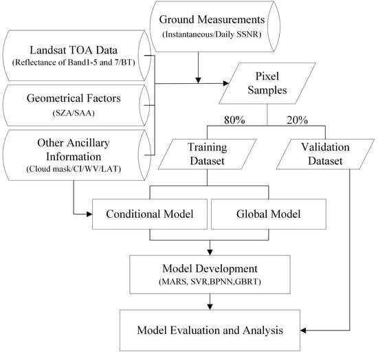
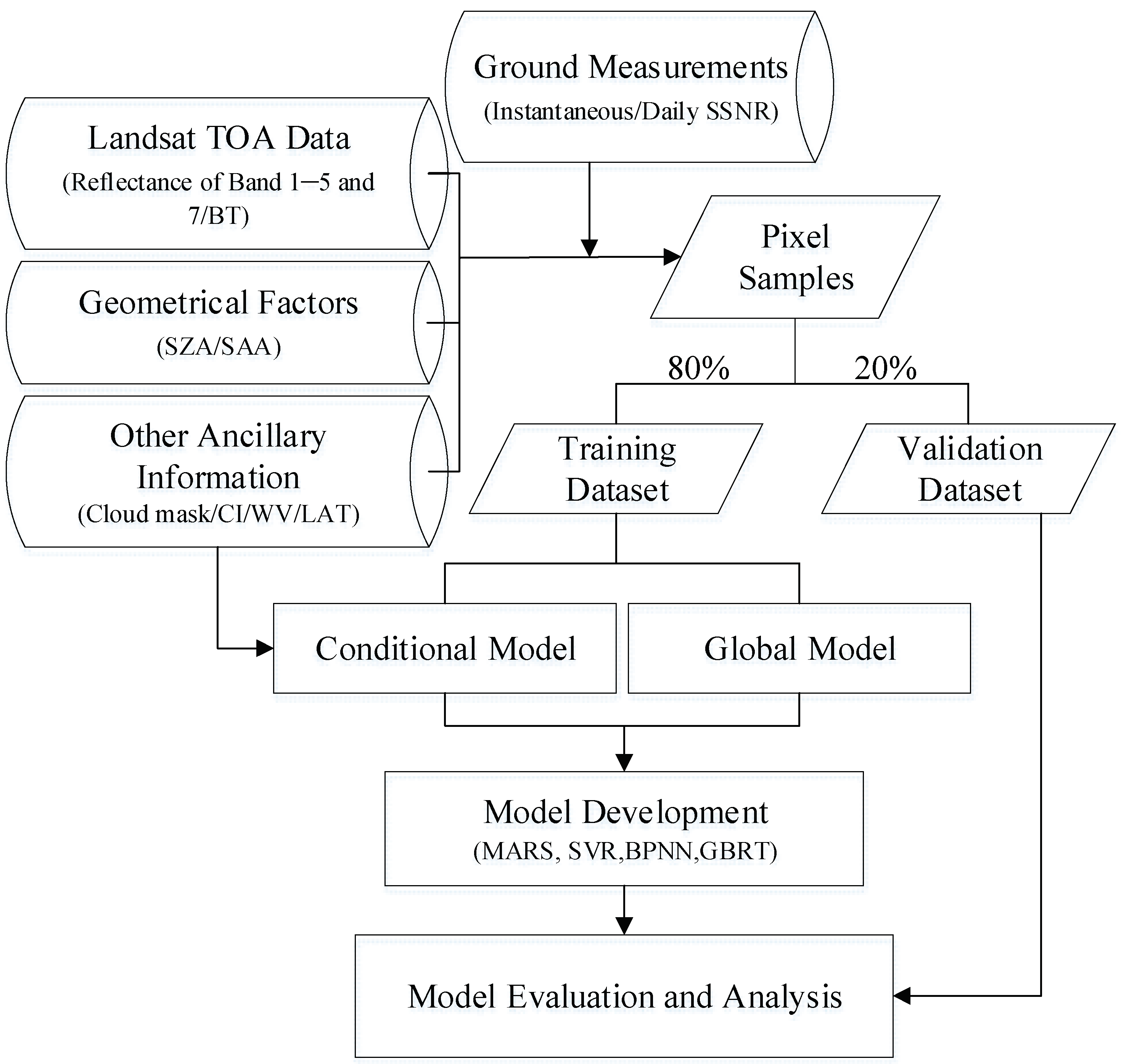
2. Data and Methods
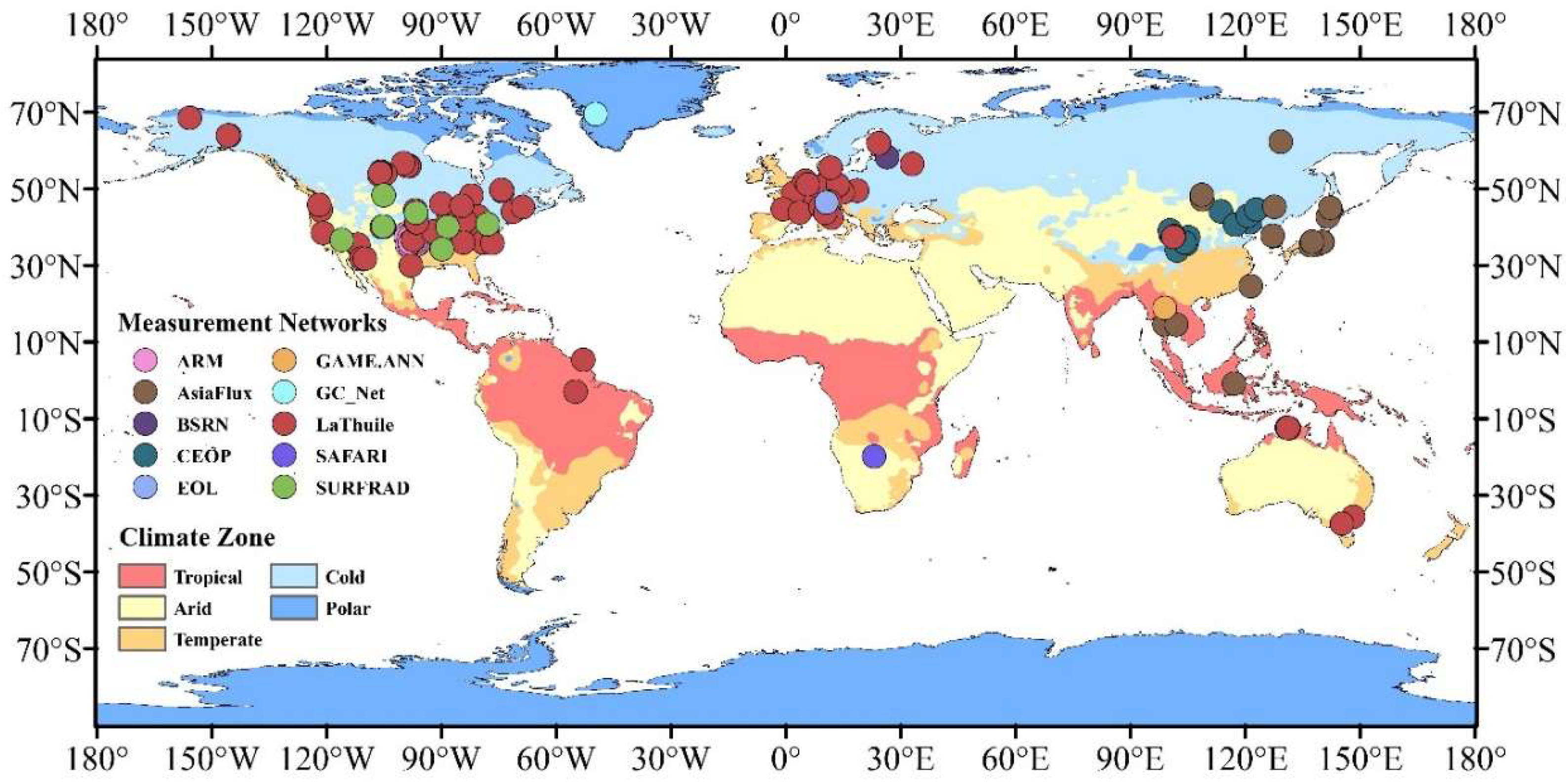
2.1. Data
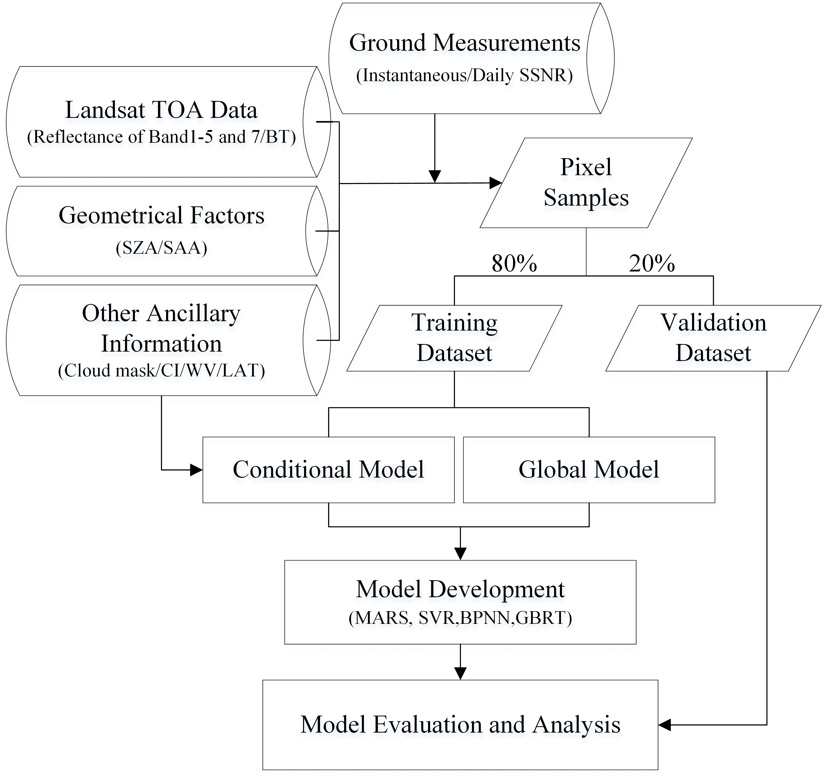
2.1.1. In-Situ Measurements
2.1.2. Remotely Sensed Data
2.1.3. MERRA-2 Reanalysis Data
2.1.4. Other Parameters
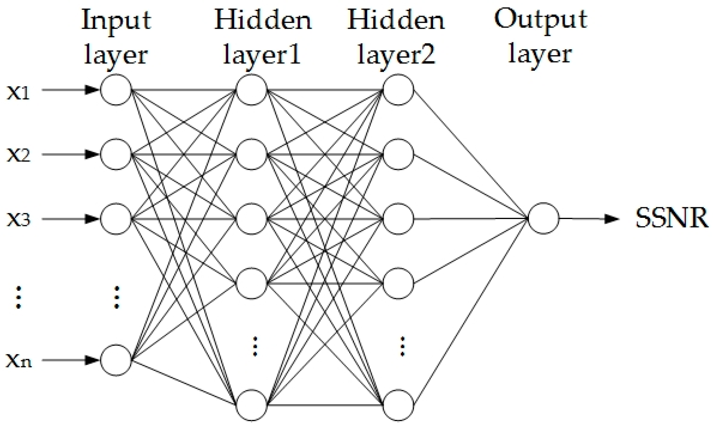
2.2. Methods
3. Results and Analysis
3.1. Model Development
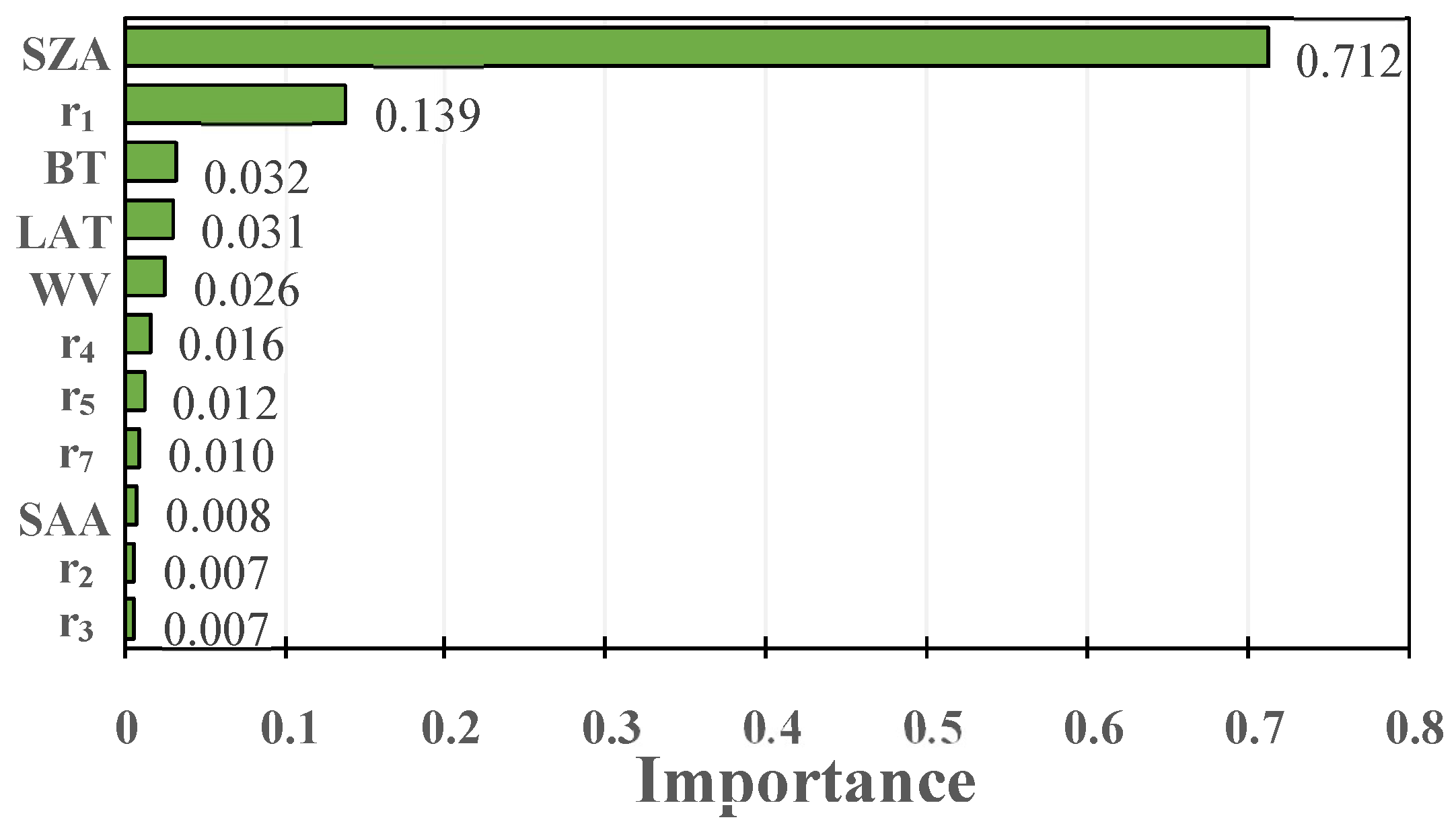
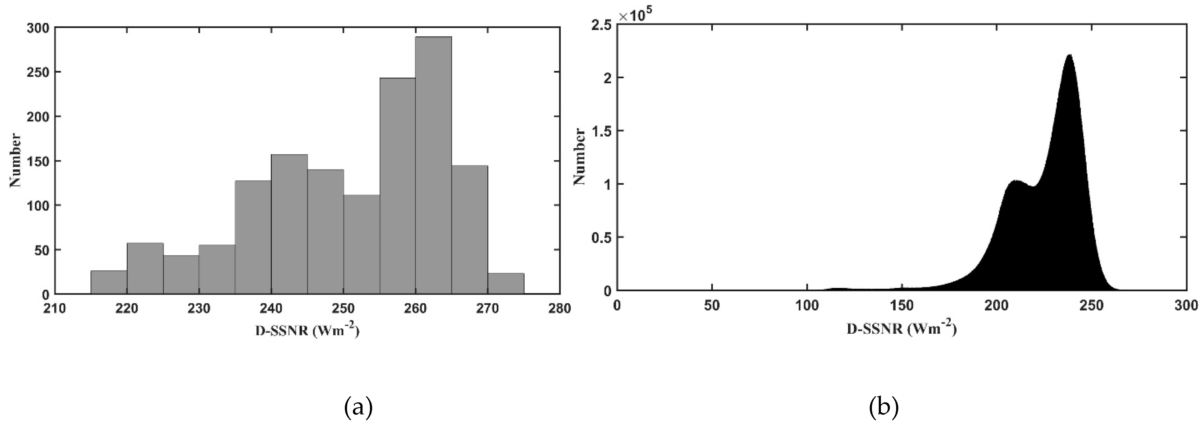
3.1.1. Ins-SSNR
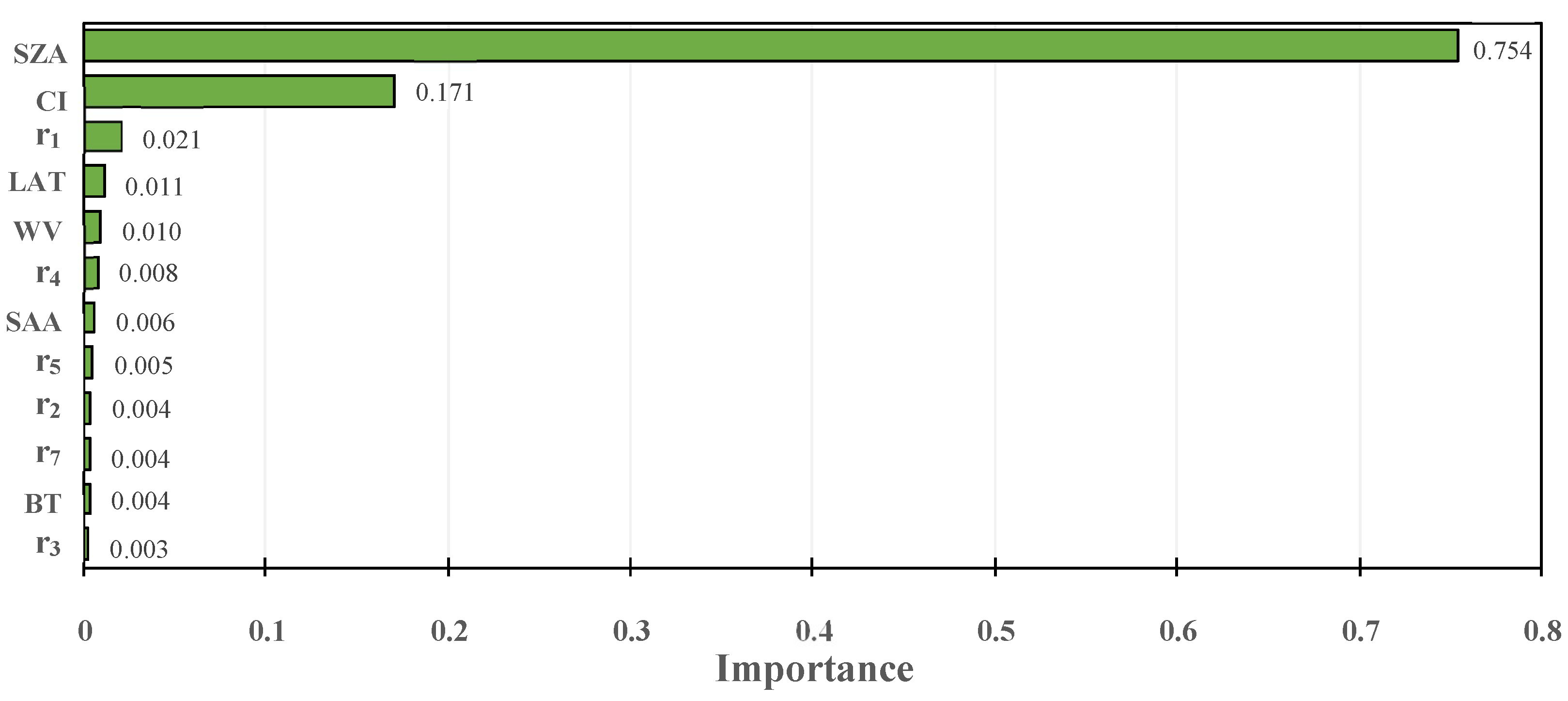
3.1.2. D-SSNR
3.2. Validation and Comparison
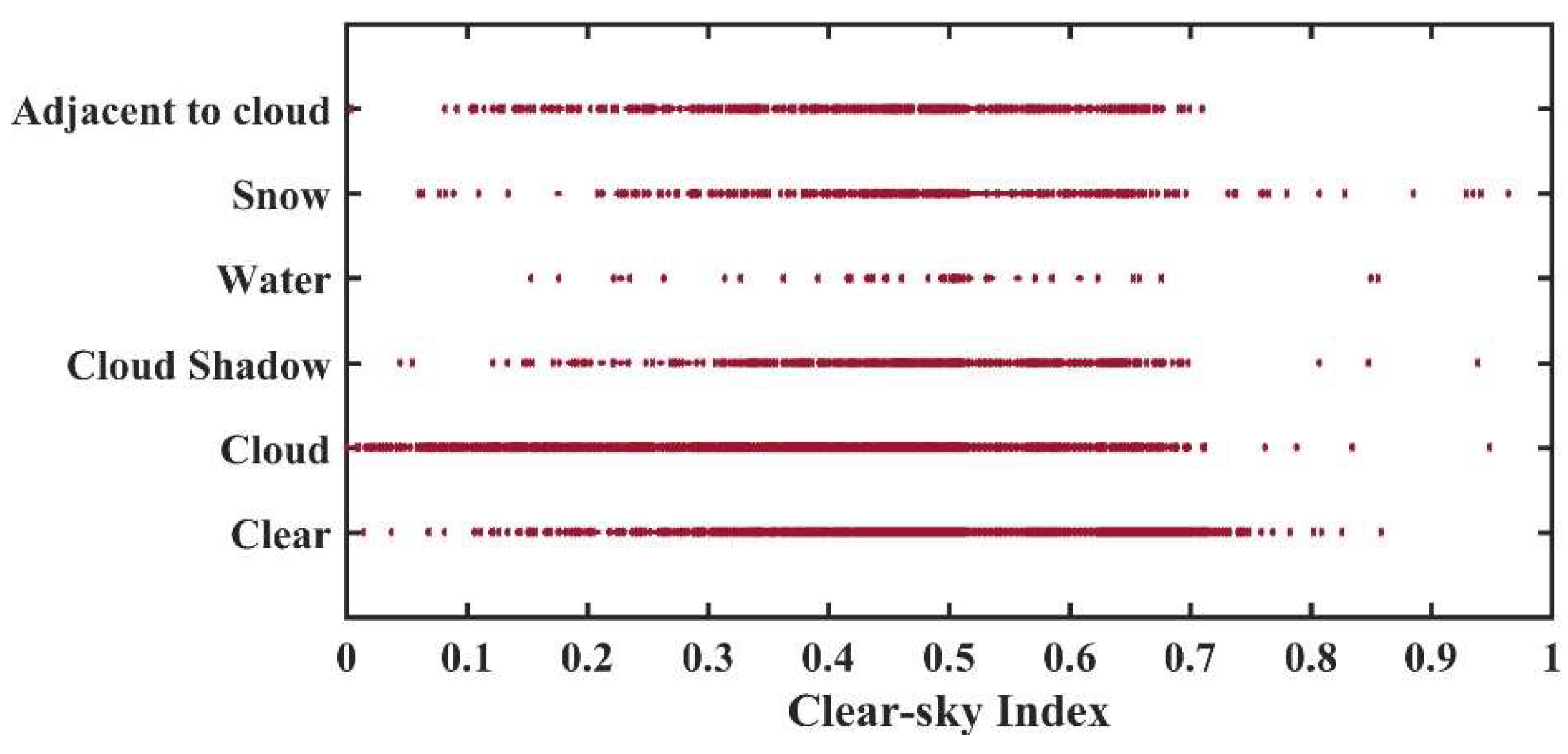
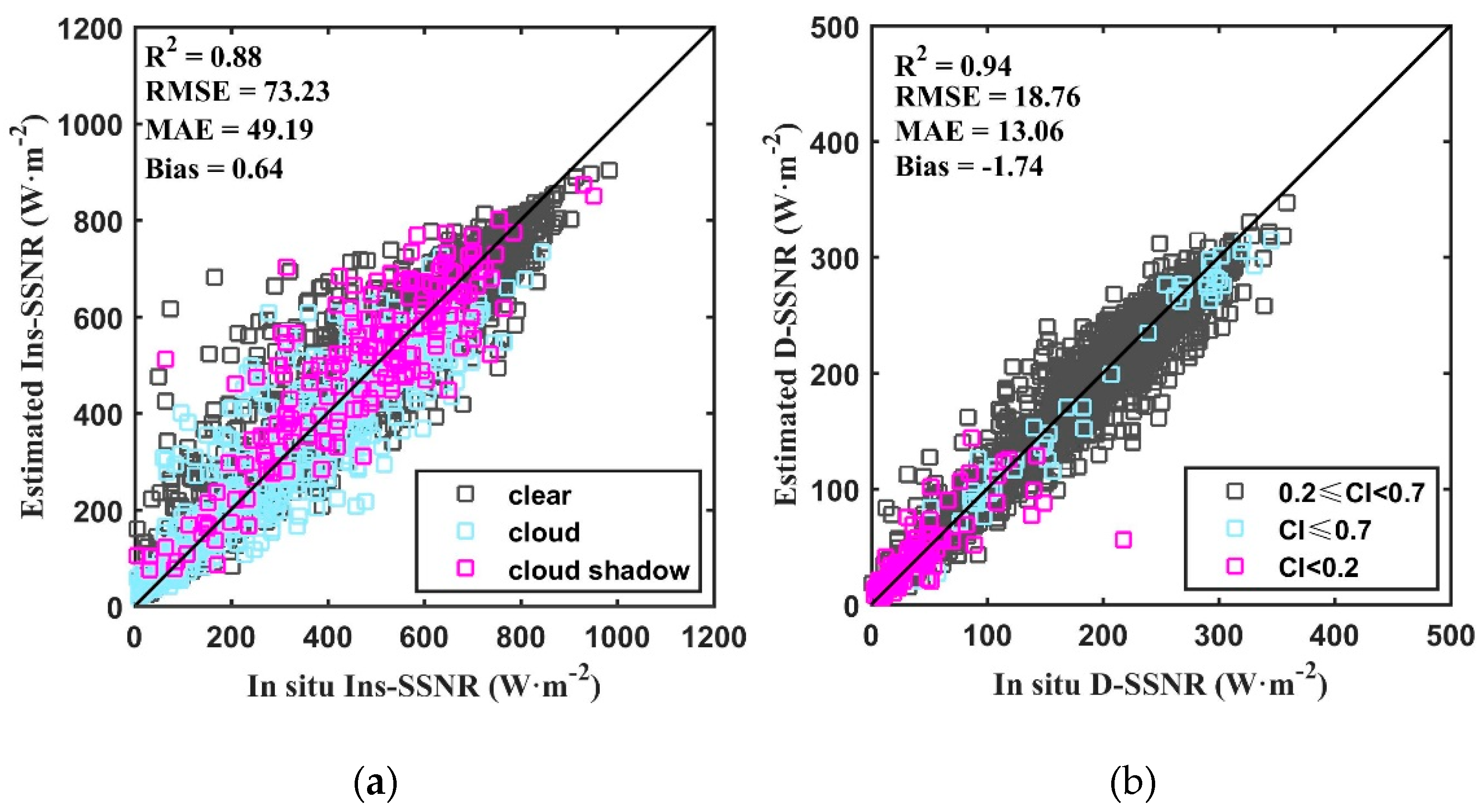
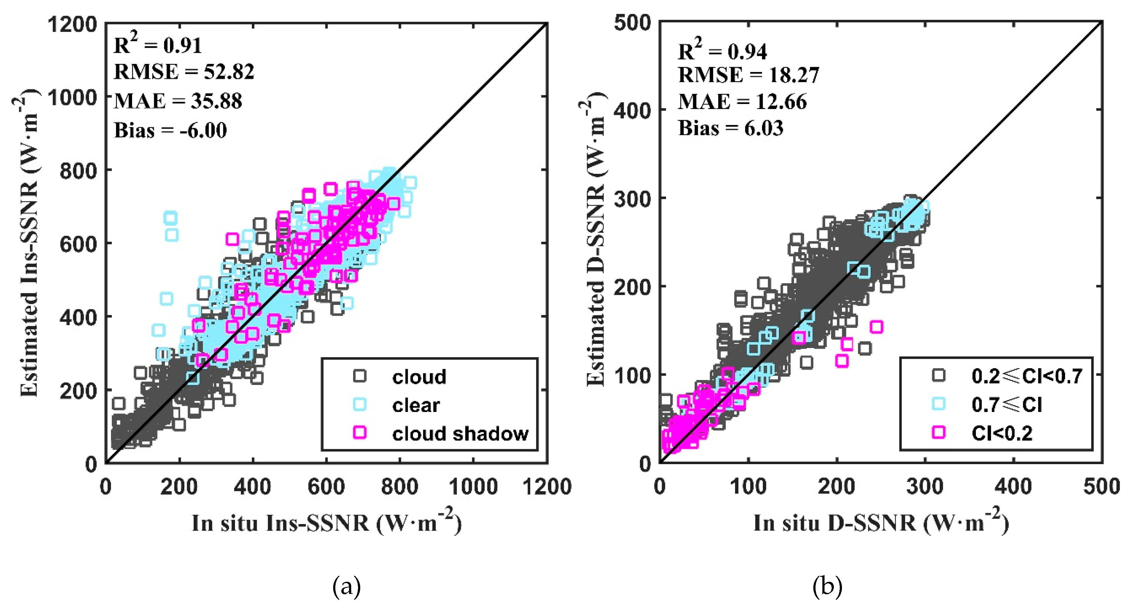
3.2.1. Direct Validation
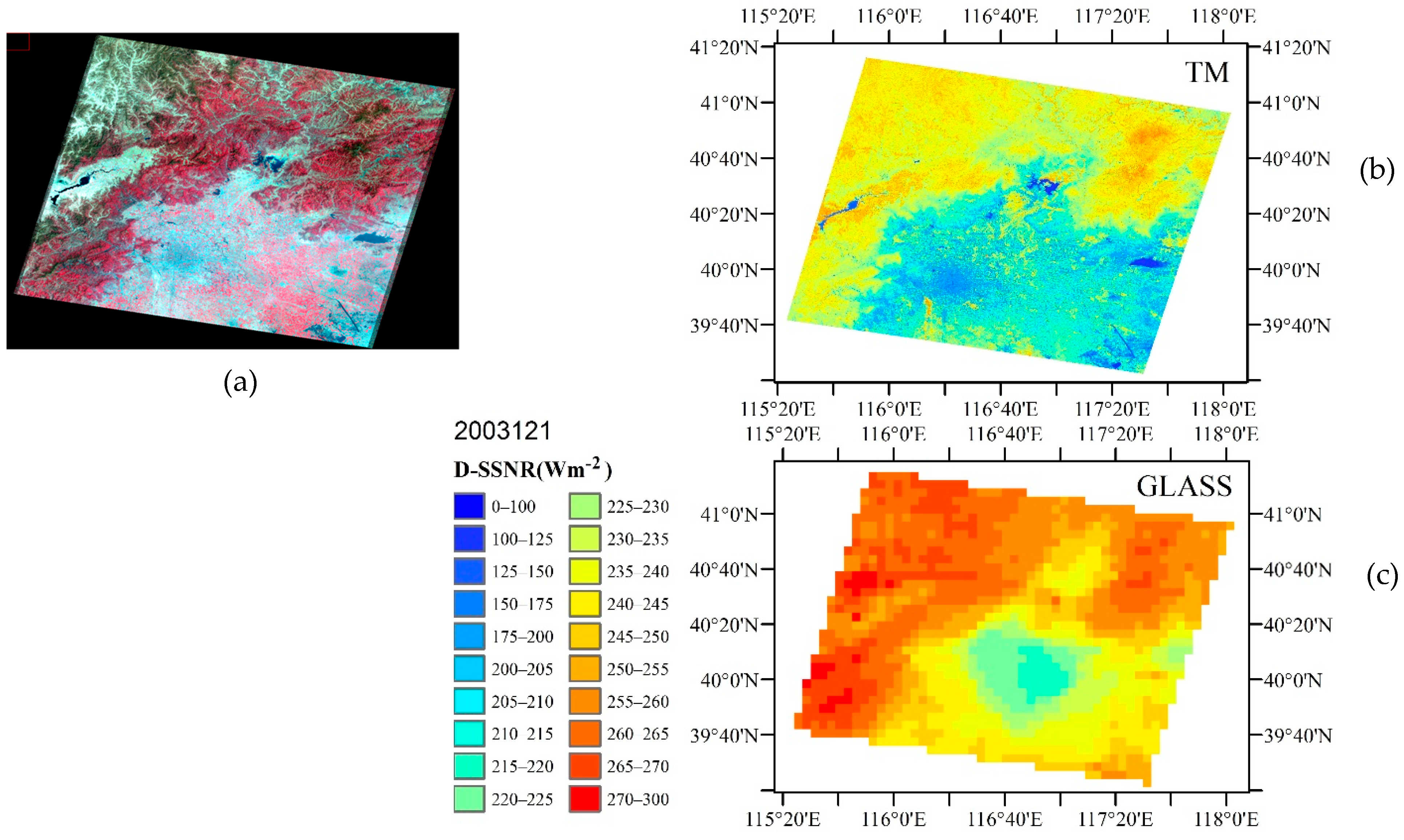
3.2.2. Comparison with GLASS Product
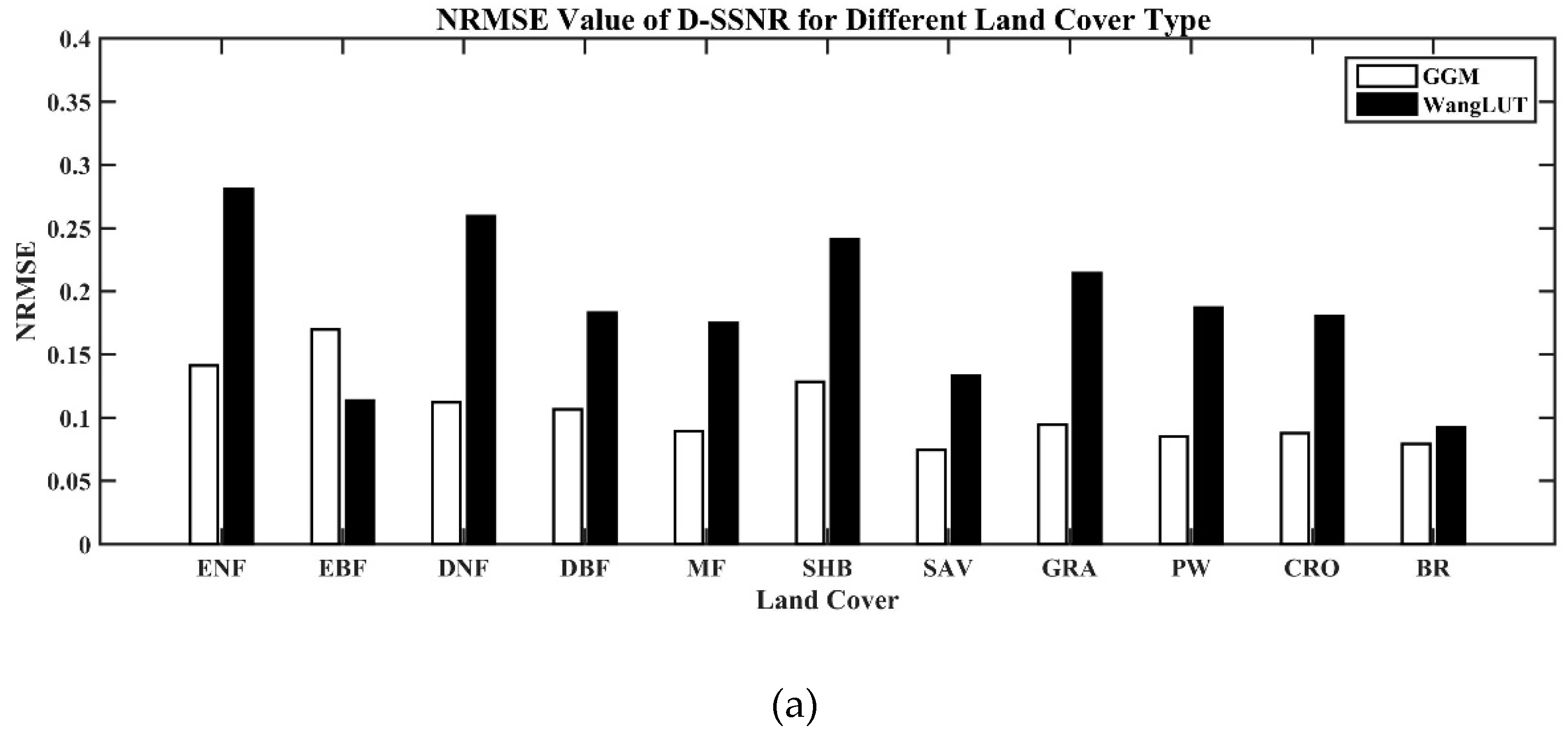
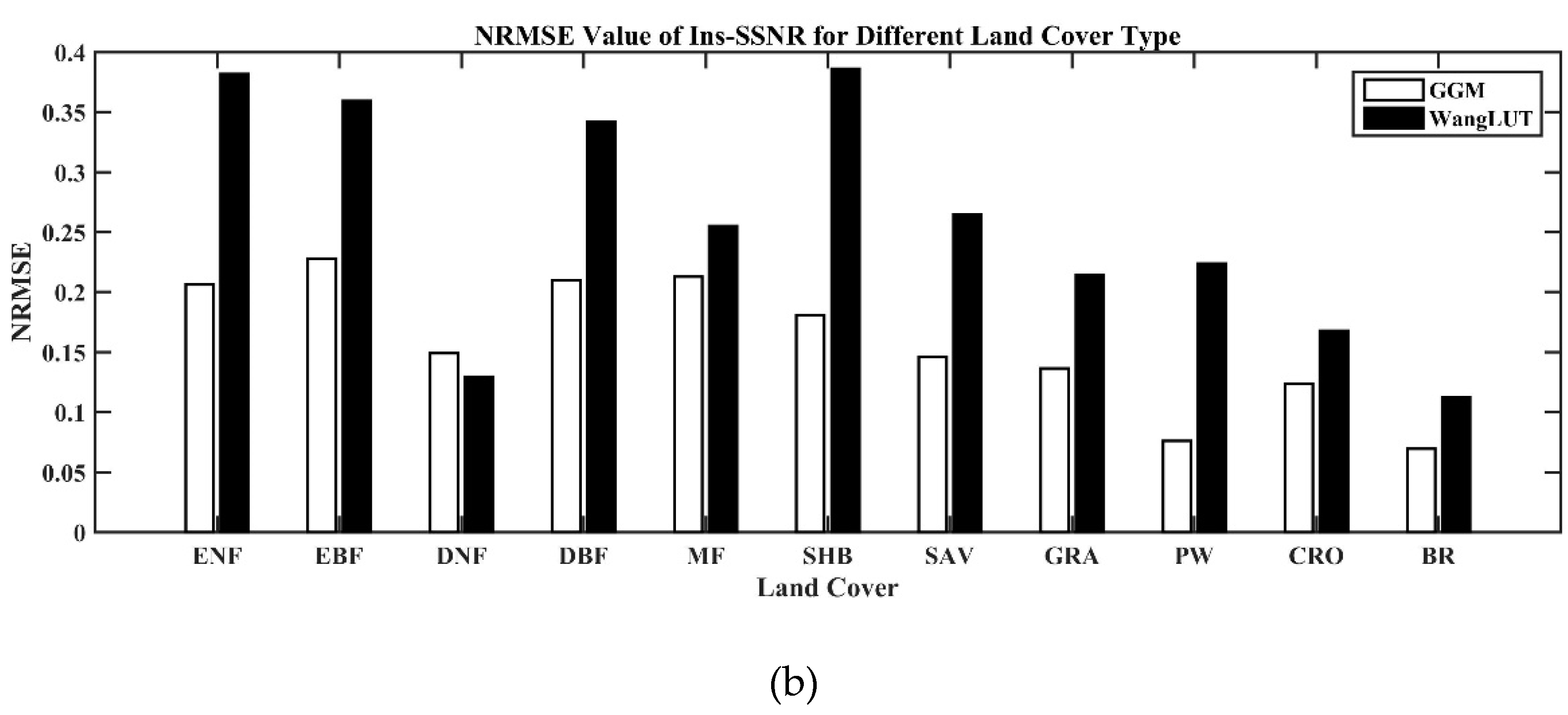
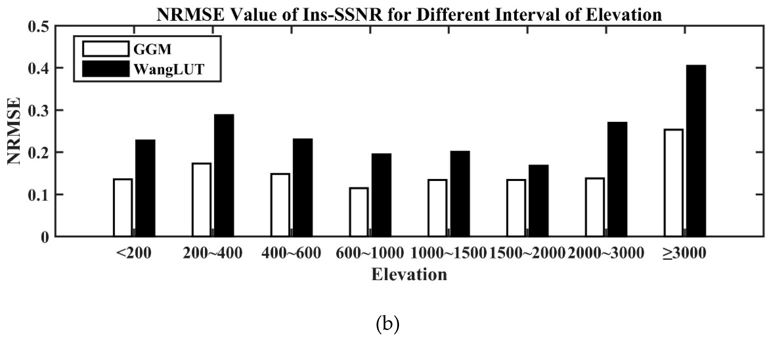
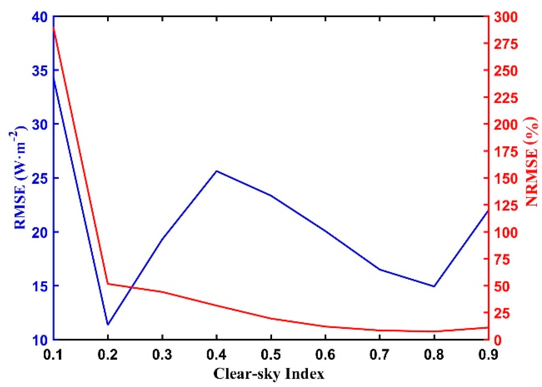
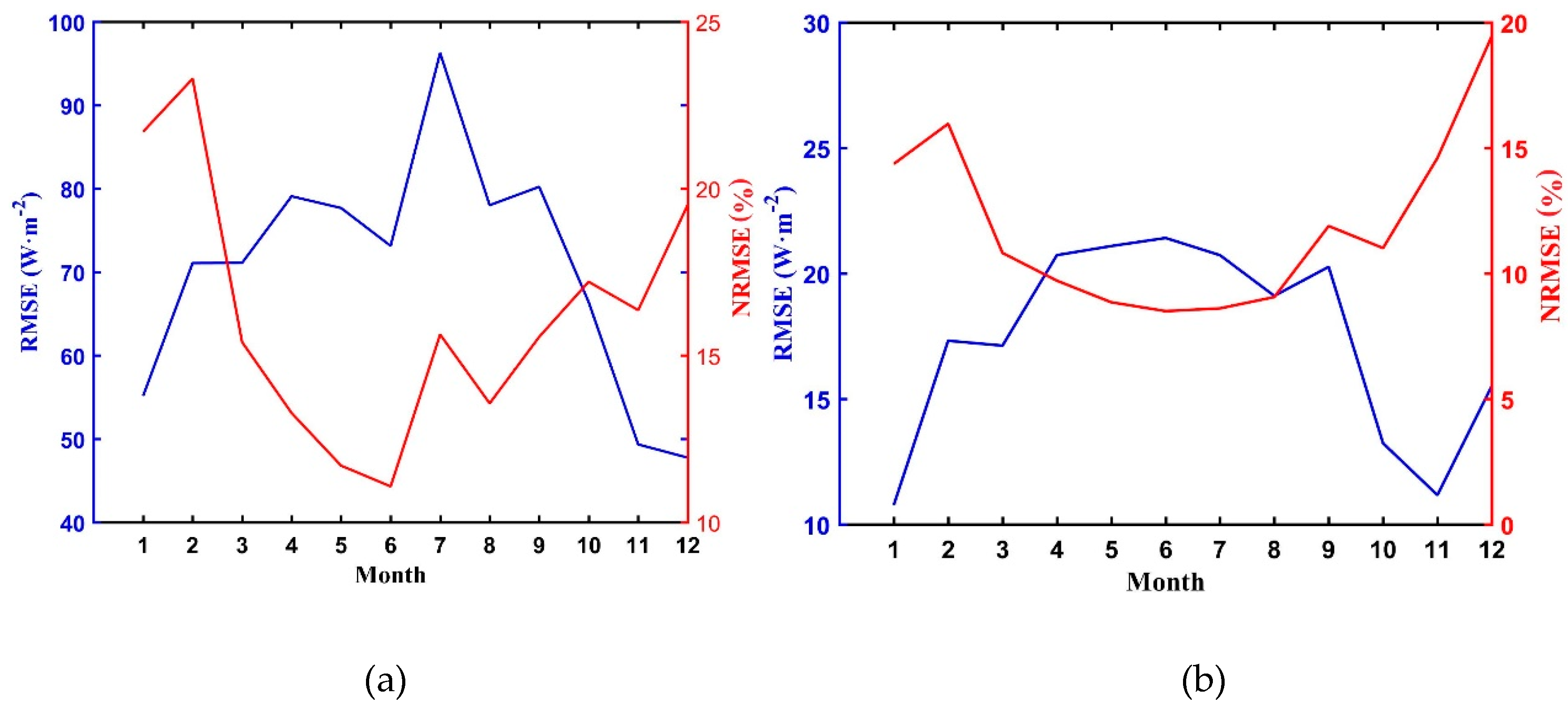
3.3. Model Performance Analysis
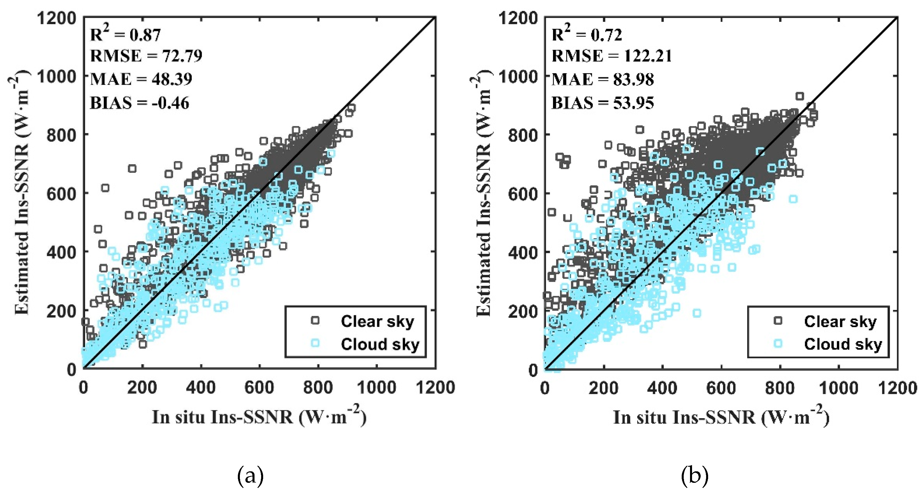
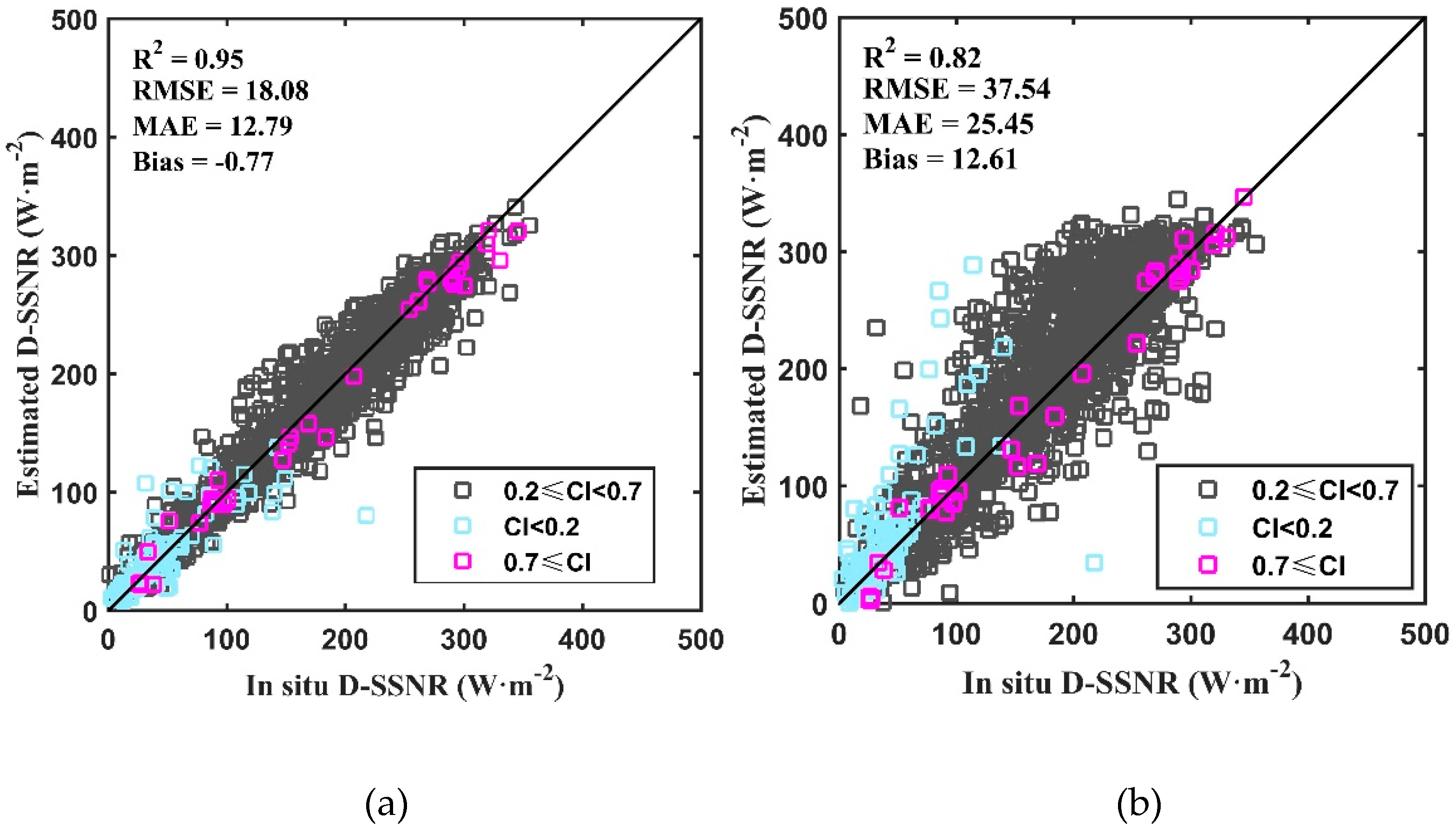
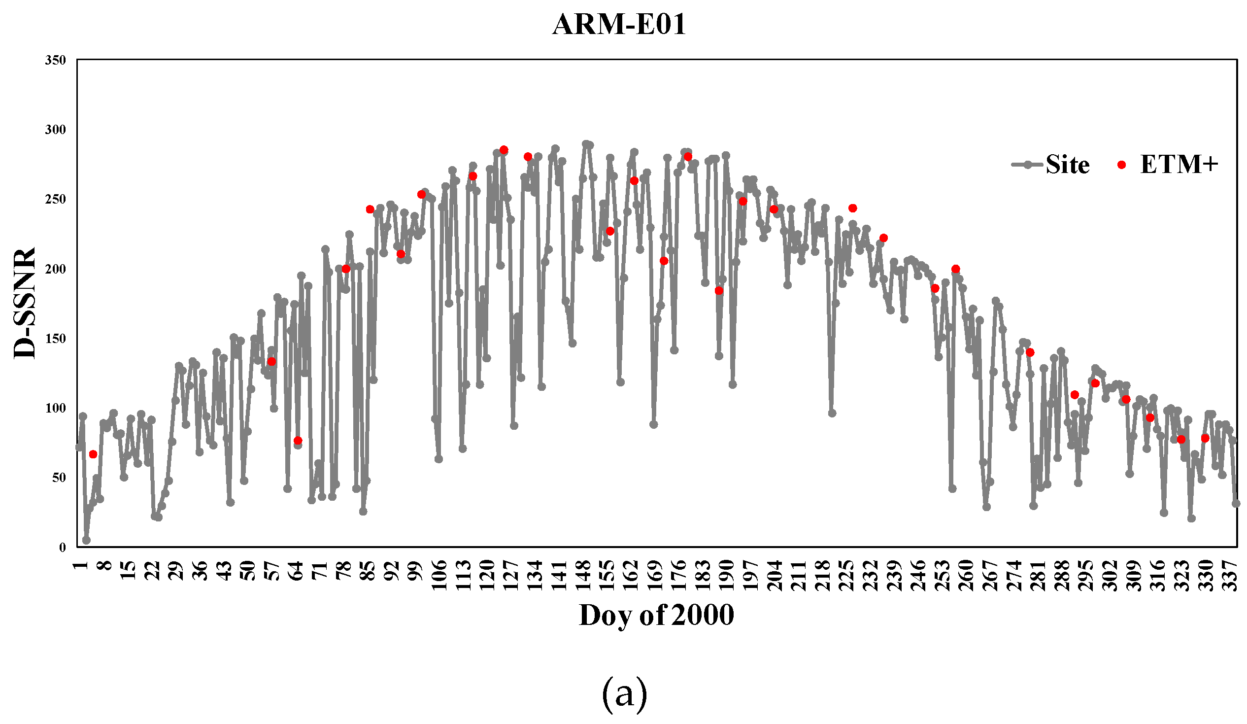
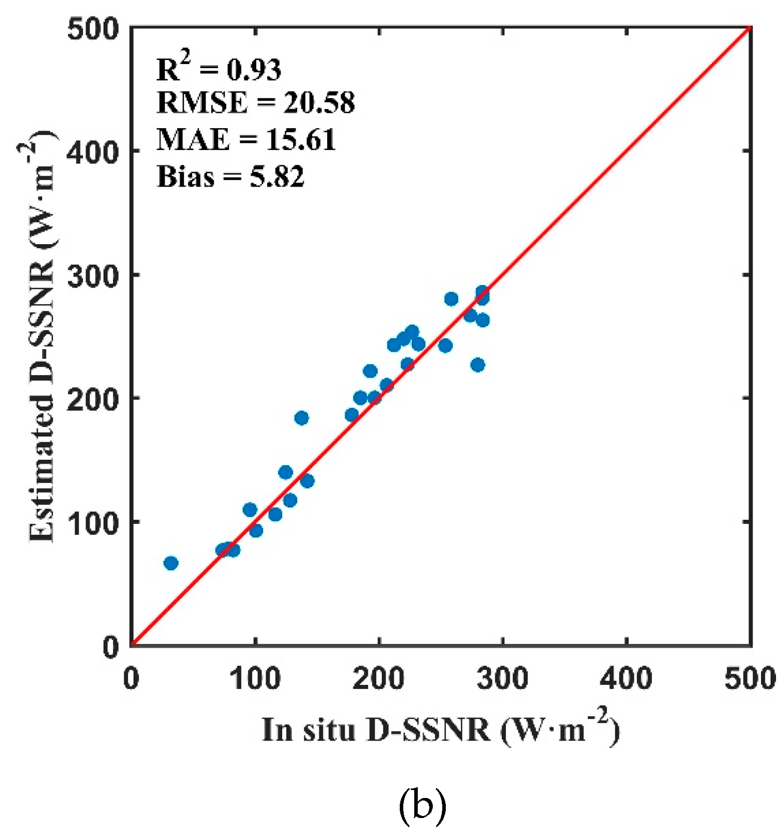
3.4. Extended Use to Landsat 7/ETM+ Data
4. Conclusions
Author Contributions
Funding
Acknowledgments
Conflicts of Interest
Appendix A

References
- Stephens, G.L.; Li, J.; Wild, M.; Clayson, C.A.; Loeb, N.; Kato, S.; L’Ecuyer, T.; Stackhouse, P.W.; Lebsock, M.; Andrews, T. An update on Earth’s energy balance in light of the latest global observations. Nat. Geosci. 2012, 5, 691–696. [Google Scholar] [CrossRef]
- Jiang, B.; Liang, S.; Ma, H.; Zhang, X.; Xiao, Z.; Zhao, X.; Jia, K.; Yao, Y.; Jia, A. GLASS Daytime All-Wave Net Radiation Product: Algorithm Development and Preliminary Validation. Remote Sens. 2016, 8, 222. [Google Scholar] [CrossRef]
- Liang, S.; Zhao, X.; Liu, S.; Yuan, W.; Cheng, X.; Xiao, Z.; Zhang, X.; Liu, Q.; Cheng, J.; Tang, H.; et al. A long-term Global LAnd Surface Satellite (GLASS) data-set for environmental studies. Int. J. Digit. Earth 2013, 6, 5–33. [Google Scholar] [CrossRef]
- Pellicciotti, F.; Brock, B.; Strasser, U.; Burlando, P.; Funk, M.; Corripio, J. An enhanced temperature-index glacier melt model including the shortwave radiation balance: development and testing for Haut Glacier d’Arolla, Switzerland. J. Glaciol. 2005, 51, 573–587. [Google Scholar] [CrossRef]
- Allan, R.; Pereira, L.; Raes, D.; Smith, M. Crop Evapotranspiration-Guidelines for Computing Crop Water Requirements-FAO Irrigation and Drainage Paper 56; FAO: Rome, Italy, 1998; Volume 56. [Google Scholar]
- Zhao, W.; Li, Z.-L. Sensitivity study of soil moisture on the temporal evolution of surface temperature over bare surfaces. Int. J. Remote Sens. 2013, 34, 3314–3331. [Google Scholar] [CrossRef]
- Cess, R.D.; Vulis, I.L. Inferring Surface Solar Absorption from Broadband Satellite Measurements. J. Clim. 1989, 2, 974–985. [Google Scholar] [CrossRef]
- Cess, R.D.; Dutton, E.G.; Deluisi, J.J.; Jiang, F. Determining Surface Solar Absorption from Broadband Satellite Measurements for Clear Skies: Comparison with Surface Measurements. J. Clim. 1991, 4, 236–247. [Google Scholar] [CrossRef]
- Li, Z.; Leighton, H.G.; Masuda, K.; Takashima, T. Estimation of SW Flux Absorbed at the Surface from TOA Reflected Flux. J. Clim. 1993, 6, 317–330. [Google Scholar] [CrossRef]
- Tang, B.; Li, Z.-L.; Zhang, R. A direct method for estimating net surface shortwave radiation from MODIS data. Remote Sens. Environ. 2006, 103, 115–126. [Google Scholar] [CrossRef]
- Huang, G.; Liu, S.; Liang, S. Estimation of net surface shortwave radiation from MODIS data. Int. J. Remote Sens. 2012, 33, 804–825. [Google Scholar] [CrossRef]
- Wang, D.; Liang, S.; He, T.; Shi, Q. Estimation of Daily Surface Shortwave Net Radiation From the Combined MODIS Data. IEEE Trans. Geosci. Remote Sens. 2015, 53, 5519–5529. [Google Scholar] [CrossRef]
- Inamdar, A.; Guillevic, P. Net Surface Shortwave Radiation from GOES Imagery—Product Evaluation Using Ground-Based Measurements from SURFRAD. Remote Sens. 2015, 7, 10788–10814. [Google Scholar] [CrossRef]
- Zhang, X.; Li, L. Estimating net surface shortwave radiation from Chinese geostationary meteorological satellite FengYun-2D (FY-2D) data under clear sky. Opt. Express 2016, 24, A476–A487. [Google Scholar] [CrossRef] [PubMed]
- Wild, M.; Folini, D.; Schär, C.; Loeb, N.; Dutton, E.G.; König-Langlo, G. The global energy balance from a surface perspective. Clim. Dyn. 2013, 40, 3107–3134. [Google Scholar] [CrossRef]
- Liang, S.; Wang, K.; Zhang, X.; Wild, M. Review on Estimation of Land Surface Radiation and Energy Budgets From Ground Measurement, Remote Sensing and Model Simulations. IEEE J. Sel. Top. Appl. Earth Obs. Remote Sens. 2010, 3, 225–240. [Google Scholar] [CrossRef]
- Tarpley, J.D. Estimating Incident Solar Radiation at the Surface from Geostationary Satellite Data. J. Appl. Meteorol. 1979, 18, 1172–1181. [Google Scholar] [CrossRef]
- Kim, H.-Y.; Liang, S. Development of a hybrid method for estimating land surface shortwave net radiation from MODIS data. Remote Sens. Environ. 2010, 114, 2393–2402. [Google Scholar] [CrossRef]
- He, T.; Liang, S.; Wang, D.; Shi, Q.; Goulden, M.L. Estimation of high-resolution land surface net shortwave radiation from AVIRIS data: Algorithm development and preliminary results. Remote Sens. Environ. 2015, 167, 20–30. [Google Scholar] [CrossRef]
- Duan, S.-B.; Li, Z.-L.; Leng, P. A framework for the retrieval of all-weather land surface temperature at a high spatial resolution from polar-orbiting thermal infrared and passive microwave data. Remote Sens. Environ. 2017, 195, 107–117. [Google Scholar] [CrossRef]
- Zhang, X.; Wang, D.; Liu, Q.; Yao, Y.; Jia, K.; He, T.; Jiang, B.; Wei, Y.; Ma, H.; Zhao, X.; et al. An Operational Approach for Generating the Global Land Surface Downward Shortwave Radiation Product From MODIS Data. IEEE Trans. Geosci. Remote Sens. 2019, 57, 4636–4650. [Google Scholar] [CrossRef]
- Zhang, X.; Liang, S.; Zhou, G.; Wu, H.; Zhao, X. Generating Global LAnd Surface Satellite incident shortwave radiation and photosynthetically active radiation products from multiple satellite data. Remote Sens. Environ. 2014, 152, 318–332. [Google Scholar] [CrossRef]
- Hansen, M.C.; Krylov, A.; Tyukavina, A.; Potapov, P.V.; Turubanova, S.; Zutta, B.; Ifo, S.; Margono, B.; Stolle, F.; Moore, R. Humid tropical forest disturbance alerts using Landsat data. Environ. Res. Lett. 2016, 11, 034008. [Google Scholar] [CrossRef]
- Zhou, J.; Hu, D.; Weng, Q. Analysis of surface radiation budget during the summer and winter in the metropolitan area of Beijing, China. J. Appl. Remote Sens. 2010, 4, 183–192. [Google Scholar]
- Pun, M.; Mutiibwa, D.; Li, R. Land Use Classification: A Surface Energy Balance and Vegetation Index Application to Map and Monitor Irrigated Lands. Remote Sens. 2017, 9, 1256. [Google Scholar] [CrossRef]
- Wang, D.; Liang, S. Estimating Top-of-Atmosphere Daily Reflected Shortwave Radiation Flux Over Land From MODIS Data. IEEE Trans. Geosci. Remote Sens. 2017, 55, 4022–4031. [Google Scholar] [CrossRef]
- Wild, M. Solar radiation budgets in atmospheric model intercomparisons from a surface perspective. Geophys. Res. Lett. 2005, 32. [Google Scholar] [CrossRef]
- Wild, M. Towards Global Estimates of the Surface Energy Budget. Curr. Clim. Chang. Rep. 2017, 3, 87–97. [Google Scholar] [CrossRef]
- Tucker, C.J.; Grant, D.M.; Dykstra, J.D. NASA’s Global Orthorectified Landsat Data Set. Photogramm. Eng. Remote Sens. 2004, 70, 313–322. [Google Scholar] [CrossRef]
- Dubayah, R. Estimating net solar radiation using Landsat Thematic Mapper and digital elevation data. Water Resour. Res. 1992, 28, 2469–2484. [Google Scholar] [CrossRef]
- Duguay, C.R. An approach to the estimation of surface net radiation in mountain areas using remote sensing and digital terrain data. Theor. Appl. Climatol. 1995, 52, 55–68. [Google Scholar] [CrossRef]
- Wang, D.; Liang, S.; He, T. Mapping High-Resolution Surface Shortwave Net Radiation From Landsat Data. IEEE Geosci. Remote Sens. Lett. 2014, 11, 459–463. [Google Scholar] [CrossRef]
- Wu, H.; Ying, W. Benchmarking Machine Learning Algorithms for Instantaneous Net Surface Shortwave Radiation Retrieval Using Remote Sensing Data. Remote Sens. 2019, 11, 2520. [Google Scholar] [CrossRef] [Green Version]
- U.S. Department of Energy. ARM-Data. Available online: http://www.archive.arm.gov/ (accessed on 7 November 2014).
- AsiaFlux. Available online: http://www.asiaflux.net/ (accessed on 7 November 2014).
- BSRN-World Radiation Monitoring Center Baseline Surface Radiation Network. Available online: http://www.bsrn.awi.de/ (accessed on 7 November 2014).
- Citterio, M.; Diolaiuti, G.; Smiraglia, C. Initial results from the Automatic Weather Station (AWS) on the ablation tongue of Forni Glacier (Upper Valtellina, Italy). Geogr. Fis. E Din. Quat. 2007, 30, 141–151. [Google Scholar]
- Steffen, K.; Box, J.E.; Abdalati, W. Greenland Climate Network: GC-Net; CRREL Special Report 96-27; US ArmyCold Regions Research and Engineering Laboratory: Hanover, NH, USA, 1996. [Google Scholar]
- Fluxnet. Available online: http://www.fluxdata.org/ (accessed on 7 November 2014).
- Lloyd, J.; Kolle, O.; Veenendaal, E.M.; Arneth, A.; Wolski, P. SAFARI 2000 Meteorological and Flux Tower Measurements in Maun, Botswana, 2000; ORNL Distributed Active Archive Center: Oak Ridge, TN, USA, 2004. [Google Scholar] [CrossRef]
- Privette, J.L.; Mukelabai, M.M.; Hanan, N.P.; Hao, Z. SAFARI 2000 Surface Albedo and Radiation Fluxes at Mongu and Skukuza, 2000-2002; ORNL Distributed Active Archive Center: Oak Ridge, TN, USA, 2005. [Google Scholar] [CrossRef]
- ESRL Global Mnotoring Division. Available online: http://www.esrl.noaa.gov/gmd/grad/surfrad/ (accessed on 7 November 2014).
- Ohmura, A.; Gilgen, H.; Hegner, H.; Müller, G.; Wild, M.; Dutton, E.G.; Forgan, B.; Fröhlich, C.; Philipona, R.; Heimo, A. Baseline Surface Radiation Network (BSRN/WCRP): New Precision Radiometry for Climate Research. Bull. Am. Meteorol. Soc. 1998, 79, 215–2136. [Google Scholar] [CrossRef] [Green Version]
- Xu, Z.; Liu, S.; Li, X.; Shi, S.; Wang, J.; Zhu, Z.; Xu, T.; Wang, W.; Ma, M. Intercomparison of surface energy flux measurement systems used during the HiWATER-MUSOEXE. J. Geophys. Res. Atmos. 2013, 118, 13–140. [Google Scholar] [CrossRef]
- Jia, Z.; Liu, S.; Xu, Z.; Chen, Y.; Zhu, M. Validation of remotely sensed evapotranspiration over the Hai River Basin, China. J. Geophys. Res. Atmos. 2012, 117. [Google Scholar] [CrossRef]
- Steffen, K.; Box, J. Surface climatology of the Greenland Ice Sheet: Greenland Climate Network 1995–1999. J. Geophys. Res. Atmos. 2001, 106, 33951–33964. [Google Scholar] [CrossRef]
- Augustine, J.A.; DeLuisi, J.J.; Long, C.N. SURFRAD–A National Surface Radiation Budget Network for Atmospheric Research. Bull. Am. Meteorol. Soc. 2000, 81, 2341–2358. [Google Scholar] [CrossRef] [Green Version]
- Peel, M.C.; Finlayson, B.L.; Mcmahon, T.A. Updated world map of the Köppen-Geiger climate classification. Hydrol. Earth Syst. Sci. Discuss. 2007, 11, 1633–1644. [Google Scholar] [CrossRef] [Green Version]
- Jiang, B.; Zhang, Y.; Liang, S.; Wohlfahrt, G.; Arain, A.; Cescatti, A.; Georgiadis, T.; Jia, K.; Kiely, G.; Lund, M.; et al. Empirical estimation of daytime net radiation from shortwave radiation and ancillary information. Agric. For. Meteorol. 2015, 211-212, 23–36. [Google Scholar] [CrossRef] [Green Version]
- White, K.; Robinson, G.J. Estimating surface net solar radiation by use of Landsat-5 TM and digital elevation models. Int. J. Remote Sens. 2000, 21, 31–43. [Google Scholar] [CrossRef]
- Goodin, D.G. Mapping the surface radiation budget and net radiation in a sand hills wetland using a combined modeling/ remote sensing method and Landsat thematic Mapper Imagery. Geocarto Int. 1995, 10, 19–29. [Google Scholar] [CrossRef]
- Mallick, J.; Kant, Y.; Bharath, B.D. Estimation of land surface temperature over Delhi using Landsat-7 ETM+. J. Indian Geophys. Union 2008, 12, 131–140. [Google Scholar]
- He, T.; Liang, S.; Wang, D.; Shuai, Y.; Yu, Y. Fusion of Satellite Land Surface Albedo Products Across Scales Using a Multiresolution Tree Method in the North Central United States. IEEE Trans. Geosci. Remote Sens. 2014, 52, 3428–3439. [Google Scholar] [CrossRef]
- Claverie, M.; Vermote, E.F.; Franch, B.; Masek, J.G. Evaluation of the Landsat-5 TM and Landsat-7 ETM+ surface reflectance products. Remote Sens. Environ. 2015, 169, 390–403. [Google Scholar] [CrossRef]
- Masek, J.G.; Vermote, E.F.; Saleous, N.E.; Wolfe, R.; Hall, F.G.; Huemmrich, K.F.; Feng, G.; Kutler, J.; Teng-Kui, L. A Landsat surface reflectance dataset for North America, 1990-2000. IEEE Geosci. Remote Sens. Lett. 2006, 3, 68–72. [Google Scholar] [CrossRef]
- Zhu, Z.; Woodcock, C.E. Object-based cloud and cloud shadow detection in Landsat imagery. Remote Sens. Environ. 2012, 118, 83–94. [Google Scholar] [CrossRef]
- Melaas, E.K.; Friedl, M.A.; Zhu, Z. Detecting interannual variation in deciduous broadleaf forest phenology using Landsat TM/ETM+ data. Remote Sens. Environ. 2013, 132, 176–185. [Google Scholar] [CrossRef]
- Chander, G.; Markham, B. Revised Landsat-5 TM radiometric calibration procedures and postcalibration dynamic ranges. IEEE Trans. Geosci. Remote Sens. 2003, 41, 2674–2677. [Google Scholar] [CrossRef] [Green Version]
- Roy, D.P.; Kovalskyy, V.; Zhang, H.K.; Vermote, E.F.; Yan, L.; Kumar, S.S.; Egorov, A. Characterization of Landsat-7 to Landsat-8 reflective wavelength and normalized difference vegetation index continuity. Remote Sens. Environ. 2016, 185, 57–70. [Google Scholar] [CrossRef] [Green Version]
- Liu, Q.; Wang, L.; Qu, Y.; Liu, N.; Liu, S.; Tang, H.; Liang, S. Preliminary evaluation of the long-term GLASS albedo product. Int. J. Digit. Earth 2013, 6, 69–95. [Google Scholar] [CrossRef]
- Wu, X.; Xiao, Q.; Wen, J.; Ma, M.; Dongqin, Y. Evaluation of the MODIS and GLASS albedo products over the Heihe river Basin, China. In Proceedings of the 2016 IEEE International Geoscience and Remote Sensing Symposium (IGARSS), Beijing, China, 10–15 July 2016; pp. 3493–3495. [Google Scholar]
- Huang, G.; Wang, W.; Zhang, X.; Liang, S.; Liu, S.; Zhao, T.; Feng, J.; Ma, Z. Preliminary validation of GLASS-DSSR products using surface measurements collected in arid and semi-arid regions of China. Int. J. Digit. Earth 2013, 6, 50–68. [Google Scholar] [CrossRef]
- Bosilovich, M. The Climate Data Guide: NASA’s MERRA2 Reanalysis. Available online: https://climatedataguide.ucar.edu/climate-data/nasas-merra2-reanalysis (accessed on 1 November 2017).
- Rienecker, M.M.; Suarez, M.J.; Gelaro, R.; Todling, R.; Bacmeister, J.; Liu, E.; Bosilovich, M.G.; Schubert, S.D.; Takacs, L.; Kim, G.-K.; et al. MERRA: NASA’s Modern-Era Retrospective Analysis for Research and Applications. J. Clim. 2011, 24, 3624–3648. [Google Scholar] [CrossRef]
- Global Modeling and Assimilation Office (GMAO). MERRA-2 tavg1_2d_slv_Nx: 2d,1-Hourly,Time-Averaged,Single-Level,Assimilation,Single-Level Diagnostics V5.12.4. Available online: https://disc.gsfc.nasa.gov/datasets/M2T1NXSLV_5.12.4/summary (accessed on 7 November 2015).
- Iziomon, M.G.; Mayer, H.; Matzarakis, A. Empirical Models for Estimating Net Radiative Flux: A Case Study for Three Mid-Latitude Sites with Orographic Variability. Astrophys. Space Sci. 2000, 273, 313–330. [Google Scholar] [CrossRef]
- Irmak, S.; Irmak, A.; Jones, J.; Howell, T.; Jacobs, J.; Allen, R.G.; Hoogenboom, G. Predicting Daily Net Radiation Using Minimum Climatological Data. J. Irrig. Drain. Eng. 2003, 129, 256–259. [Google Scholar] [CrossRef]
- Friedman, J.H. Multivariate Adaptive Regression Splines. Ann. Stat. 1991, 19, 1–67. [Google Scholar] [CrossRef]
- Goh, A.T.C. Back-propagation neural networks for modeling complex systems. Artif. Intell. Eng. 1995, 9, 143–151. [Google Scholar] [CrossRef]
- Drucker, H.; Burges, C.J.C.; Kaufman, L.; Smola, A.; Vapnik, V. Support vector regression machines. In Proceedings of the 9th International Conference on Neural Information Processing Systems, Denver, CO, USA; pp. 155–161.
- Friedman, J.H. Greedy function approximation: A gradient boosting machine. Ann. Statist. 2001, 29, 1189–1232. [Google Scholar] [CrossRef]
- Southworth, J. An assessment of Landsat TM band 6 thermal data for analysing land cover in tropical dry forest regions. Int. J. Remote Sens. 2004, 25, 689–706. [Google Scholar] [CrossRef]
- Hansen, M.C.; Defries, R.S.; Townshend, J.R.G.; Sohlberg, R. Global land cover classification at 1 km spatial resolution using a classification tree approach. Int. J. Remote Sens. 2000, 21, 1331–1364. [Google Scholar] [CrossRef]
- Zhang, X.; Liang, S.; Wild, M.; Jiang, B. Analysis of surface incident shortwave radiation from four satellite products. Remote Sens. Environ. 2015, 165, 186–202. [Google Scholar] [CrossRef]
- Milborrow, S. Earth: Multivariate Adaptive Regression Splines. 2017. [Google Scholar]
- Awad, M.; Khanna, R. Support Vector Regression. In Efficient Learning Machines: Theories, Concepts, and Applications for Engineers and System Designers; Awad, M., Khanna, R., Eds.; Apress: Berkeley, CA, USA, 2015. [Google Scholar]
- Smola, A.J.; Schölkopf, B. A tutorial on support vector regression. Stat. Comput. 2004, 14, 199–222. [Google Scholar] [CrossRef] [Green Version]
- Alexandros Karatzoglou, A.S.; Kurt, H.; Achim, Z. kernlab - An S4 Package for Kernel Methods in R. J. Stat. Softw. 2004, 11, 1–20. [Google Scholar]
- Riedmiller, M.; Braun, H. A direct adaptive method for faster backpropagation learning: the RPROP algorithm. Proceedings of IEEE International Conference on Neural Networks, San Francisco, CA, USA, 28 March–1 April 1993; pp. 586–591. [Google Scholar]
- Tasadduq, I.; Rehman, S.; Bubshait, K. Application of neural networks for the prediction of hourly mean surface temperatures in Saudi Arabia. Renew. Energy 2002, 25, 545–554. [Google Scholar] [CrossRef]
- Yang, L.; Zhang, X.; Liang, S.; Yao, Y.; Jia, K.; Jia, A. Estimating Surface Downward Shortwave Radiation over China Based on the Gradient Boosting Decision Tree Method. Remote Sens. 2018, 10, 185. [Google Scholar] [CrossRef] [Green Version]
- Hastie, T.; Tibshirani, R.; Friedman, J. The elements of Statistical Learning; Springer: New York, NY, USA, 2009. [Google Scholar]
- Ridgeway, G. Generalized Boosted Models: A guide to the gbm package. 2007. [Google Scholar]
- Chen, T.; He, T.; Michael, B.; Khotilovich, V.; Tang, Y. Xgboost: Extreme Gradient Boosting. 2015. [Google Scholar]


| Abbr. | Name | Unit | Temporal Resolution | Source | |
|---|---|---|---|---|---|
| Response variable | SSNR | Surface shortwave net radiation | instantaneous/daily | In-situ | |
| Independent variables | SZA | Solar zenith angle | degree | instantaneous | Landsat data |
| SAA | Solar azimuth angle | degree | instantaneous | Landsat data | |
| WV | Water vapor | hourly/daily | MERRA-2 | ||
| LAT | Latitude | degree | - | In-situ | |
| ri1 | Top-of-atmosphere (TOA) reflectance | \ | instantaneous | Landsat data | |
| BT | Brightness temperature | K | instantaneous | Landsat data | |
| CI2 | Clearness index | \ | daily | Calculated |
| Abbreviations | Time Period | Instrument | Reference | Temporal Resolution |
|---|---|---|---|---|
| ARM1 | 1994–2011 | Kipp&Zonen Pyrgeometer | [34] | 1 min |
| AsiaFlux | 2000–2009 | Kipp&Zonen, CM-6F | [35] | 30 min |
| BSRN2 | 1995–2011 | Eppley, PIR/Kipp&Zonen CG4 | [36] | 1 or 3 min |
| CEOP3 | 2008–2009 | - | - | 30 min |
| EOL4 | 2006–2007 | Kipp&Zonen CM21, Kipp&Zonen CG4s | [37] | 1 h |
| GC_NET5 | 1997–1998 | Li Cor Photodiode & REBS Q* 7 | [38] | 1 h |
| La Thuile6 | 1997–2011 | Kipp&Zonen Pyrgeometer, etc | [39] | 30 min |
| SAFARI.20007 | 2000 | Kipp&Zonen Pyrgeometer | [40,41] | 30 min |
| SURFRAD8 | 1995–2011 | Eppley, PIR | [42] | 3 min |
| Main Types | Total Number of Samples | |
|---|---|---|
| Instantaneous SSNR | Daily SSNR | |
| ENF1 | 2246 | 2165 |
| EBF2 | 127 | 123 |
| DNF3 | 90 | 97 |
| DBF4 | 1072 | 1004 |
| MF5 | 488 | 552 |
| PW6 | 55 | 61 |
| CRO7 | 3311 | 2619 |
| ICE8 | 9 | - |
| BR9 | 512 | 228 |
| SHB10 | 411 | 405 |
| SAV11 | 269 | 271 |
| GRA12 | 7794 | 4629 |
| Total | 16,384 | 12,154 |
| Landsat 5/TM | Landsat 7/ETM+ | ||||
|---|---|---|---|---|---|
| Band | Wavelength | Resolution | Band | Wavelength | Resolution |
| 1 | 0.45–0.52 | 30 m | 1 | 0.45–0.52 | 30 m |
| 2 | 0.52–0.60 | 30 m | 2 | 0.52–0.60 | 30 m |
| 3 | 0.63–0.69 | 30 m | 3 | 0.63–0.69 | 30 m |
| 4 | 0.76–0.90 | 30 m | 4 | 0.77–0.90 | 30 m |
| 5 | 1.55–1.75 | 30 m | 5 | 1.55–1.75 | 30 m |
| 6 | 10.40–12.50 | 120 m | 6 | 10.40–12.50 | 60 m |
| 7 | 2.08–2.35 | 30 m | 7 | 2.08–2.35 | 30 m |
| 8 | 0.520–0.900 | 15 m | |||
| BT WV | WV | BT | None | TrainingTime | Fitting Time | |||||||||||||
|---|---|---|---|---|---|---|---|---|---|---|---|---|---|---|---|---|---|---|
| R2 | RMSE (W·m-2) | MAE (W·m-2) | bias (W·m-2) | R2 | RMSE (W·m-2) | MAE (W·m-2) | bias (W·m-2) | R2 | RMSE (W·m-2) | MAE (W·m-2) | bias (W·m-2) | R2 | RMSE (W·m-2) | MAE (W·m-2) | bias (W·m-2) | |||
| MARS | 0.84 | 83.39 | 58.06 | 0.05 | 0.84 | 83.44 | 58.17 | 0.18 | 0.83 | 85.46 | 60.04 | 0.17 | 0.83 | 85.46 | 60.04 | 0.17 | 1 min | 0.01 s |
| BPNN | 0.84 | 82.85 | 57.45 | 0.20 | 0.84 | 82.19 | 57.19 | 0.04 | 0.84 | 82.97 | 57.61 | 0.22 | 0.84 | 83.80 | 57.53 | –0.04 | 35 min | 0.06 s |
| SVR | 0.85 | 80.08 | 52.04 | 7.65 | 0.85 | 80.56 | 52.34 | 8.11 | 0.85 | 81.45 | 53.67 | 7.43 | 0.85 | 82.16 | 54.22 | 7.67 | 30 min | 1 s |
| GBRT | 0.86 | 75.72 | 51.51 | –0.38 | 0.86 | 76.88 | 52.25 | –0.11 | 0.86 | 77.47 | 52.92 | –1.05 | 0.86 | 78.15 | 53.49 | –0.91 | 2 h | 0.03 s |
| GGM | GCM | ||||||||||||||||||||
|---|---|---|---|---|---|---|---|---|---|---|---|---|---|---|---|---|---|---|---|---|---|
| BT WV | BT WV | WV | BT | None | |||||||||||||||||
| Samples | R2 | RMSE (W·m-2) | MAE (W·m-2) | bias (W·m-2) | R2 | RMSE (W·m-2) | MAE (W·m-2) | bias (W·m-2) | R2 | RMSE (W·m-2) | MAE (W·m-2) | bias (W·m-2) | R2 | RMSE (W·m-2) | MAE (W·m-2) | bias (W·m-2) | R2 | RMSE (W·m-2) | MAE (W·m-2) | bias (W·m-2) | |
| Clear | 12,403 | 0.86 | 69.92 | 46.22 | –1.01 | 0.86 | 71.64 | 47.49 | 0.10 | 0.86 | 71.76 | 47.59 | –0.49 | 0.85 | 72.67 | 48.75 | –0.97 | 0.85 | 73.38 | 48.87 | –0.51 |
| Cloud | 3094 | 0.78 | 91.32 | 67.71 | –1.93 | 0.78 | 92.31 | 66.96 | –2.87 | 0.78 | 92.76 | 67.93 | –4.09 | 0.77 | 93.59 | 67.96 | –3.87 | 0.76 | 95.06 | 69.44 | –6.61 |
| Cloud shadow | 887 | 0.78 | 90.89 | 67.89 | 13.91 | 0.71 | 102.35 | 77.06 | 2.13 | 0.71 | 103.02 | 78.06 | –1.41 | 0.70 | 105.33 | 79.43 | –1.74 | 0.71 | 104.05 | 79.15 | –7.85 |
| Overall | 13,116 | 0.86 | 75.72 | 51.51 | –0.38 | 0.86 | 77.92 | 52.88 | –0.36 | 0.86 | 78.25 | 53.16 | –1.23 | 0.86 | 78.35 | 53.24 | –1.57 | 0.85 | 79.43 | 53.99 | –2.16 |
| CI | Without CI | Training Time | Fitting Time | |||||||
|---|---|---|---|---|---|---|---|---|---|---|
| R2 | RMSE (W·m-2) | MAE (W·m-2) | bias (W·m-2) | R2 | RMSE (W·m-2) | MAE (W·m-2) | Bias (W·m-2) | |||
| MARS | 0.91 | 24.10 | 15.30 | 0.04 | 0.86 | 29.13 | 20.50 | 0.19 | 1 min | 0.02 s |
| BPNN | 0.92 | 22.39 | 14.78 | –0.026 | 0.86 | 28.94 | 20.30 | 0.13 | 1.5 h | 0.03 s |
| SVR | 0.92 | 21.96 | 13.90 | 1.21 | 0.88 | 27.98 | 18.70 | 2.99 | 1.2 h | 0.80 s |
| GBRT | 0.93 | 21.01 | 14.07 | 0.12 | 0.88 | 27.21 | 18.94 | –0.35 | 2.5 h | 0.02 s |
| Samples | GGM | GCM | |||||||||||
|---|---|---|---|---|---|---|---|---|---|---|---|---|---|
| CI | CI | Without CI | |||||||||||
| R2 | RMSE (W·m-2) | MAE (W·m-2) | bias (W·m-2) | R2 | RMSE (W·m-2) | MAE (W·m-2) | bias (W·m-2) | R2 | RMSE (W·m-2) | MAE (W·m-2) | bias (W·m-2) | ||
| CI < 0.2 | 414 | 0.63 | 21.52 | 11.70 | –0.22 | 0.57 | 23.35 | 12.38 | –3.16 | 0.56 | 23.77 | 12.52 | –2.94 |
| 0.2 ≤ CI < 0.7 | 9136 | 0.92 | 20.87 | 14.19 | 0.05 | 0.92 | 21.06 | 14.55 | 0.24 | 0.87 | 27.08 | 19.42 | –2.53 |
| CI ≥ 0.7 | 172 | 0.94 | 27.56 | 14.96 | –1.74 | 0.93 | 29.52 | 18.11 | 0.93 | 0.93 | 30.09 | 17.82 | –0.66 |
| Overall | 9722 | 0.93 | 21.01 | 14.07 | 0.12 | 0.92 | 21.34 | 14.52 | 0.04 | 0.88 | 26.97 | 19.08 | –2.51 |
| Elevation Interval | Total Number of Samples | |
|---|---|---|
| Instantaneous SSNR | Daily SSNR | |
| <200 m | 582 | 370 |
| 200~400 m | 1157 | 978 |
| 400~600 m | 530 | 435 |
| 600~1000 m | 390 | 287 |
| 1000~1500 m | 242 | 156 |
| 1500~2000 m | 276 | 114 |
| 2000~3000 m | 40 | 33 |
| ≥3000 m | 51 | 59 |
| Total | 3268 | 2432 |
| Site | Lat, Lon | Land Cover | Height (m) |
|---|---|---|---|
| Larned, Kansas: E01 | 38.20N, 99.32W | Cropland | 632 |
| Hillsboro, Kansas: E02 | 38.31N, 97.30W | Grassland | 450 |
| LeRoy, Kansas: E03 | 38.20N, 95.60W | Cropland | 338 |
| Plevna, Kansas: E04 | 37.95N, 98.33W | Rangeland | 513 |
| Halstead, Kansas: E05 | 38.11N, 97.51W | Wheat | 440 |
| Towanda, Kansas: E06 | 37.84N, 97.02W | Alfalfa | 409 |
| Elk Falls, Kansas: E07 | 37.38N, 96.18W | Pasture | 283 |
| Coldwater, Kansas: E08 | 37.33N, 99.31W | Rangeland | 664 |
| Ashton, Kansas: E09 | 37.13N, 97.27W | Grassland | 386 |
| Tyro, Kansas: E10 | 37.07N, 95.79W | Alfalfa | 248 |
| Byron, Oklahoma: E11 | 36.88N, 98.29W | Alfalfa | 360 |
| Pawhuska, Oklahoma: E12 | 36.84N, 96.43W | Prairie | 331 |
© 2019 by the authors. Licensee MDPI, Basel, Switzerland. This article is an open access article distributed under the terms and conditions of the Creative Commons Attribution (CC BY) license (http://creativecommons.org/licenses/by/4.0/).
Share and Cite
Wang, Y.; Jiang, B.; Liang, S.; Wang, D.; He, T.; Wang, Q.; Zhao, X.; Xu, J. Surface Shortwave Net Radiation Estimation from Landsat TM/ETM+ Data Using Four Machine Learning Algorithms. Remote Sens. 2019, 11, 2847. https://0-doi-org.brum.beds.ac.uk/10.3390/rs11232847
Wang Y, Jiang B, Liang S, Wang D, He T, Wang Q, Zhao X, Xu J. Surface Shortwave Net Radiation Estimation from Landsat TM/ETM+ Data Using Four Machine Learning Algorithms. Remote Sensing. 2019; 11(23):2847. https://0-doi-org.brum.beds.ac.uk/10.3390/rs11232847
Chicago/Turabian StyleWang, Yezhe, Bo Jiang, Shunlin Liang, Dongdong Wang, Tao He, Qian Wang, Xiang Zhao, and Jianglei Xu. 2019. "Surface Shortwave Net Radiation Estimation from Landsat TM/ETM+ Data Using Four Machine Learning Algorithms" Remote Sensing 11, no. 23: 2847. https://0-doi-org.brum.beds.ac.uk/10.3390/rs11232847