Melting Layer Detection and Characterization based on Range Height Indicator–Quasi Vertical Profiles


Korea Institute of Civil Engineering and Building Technology, Ilsan 10223, Korea
*
Author to whom correspondence should be addressed.
Remote Sens. 2019, 11(23), 2848; https://0-doi-org.brum.beds.ac.uk/10.3390/rs11232848
Submission received: 16 October 2019
/
Revised: 27 November 2019
/
Accepted: 28 November 2019
/
Published: 29 November 2019
(This article belongs to the Special Issue Radar Polarimetry—Applications in Remote Sensing of the Atmosphere)
Abstract
:The melting layer (ML) is an important region used to describe the transition of hydrometeors from the solid to the liquid phase. It is a typical feature used to characterize the vertical structure of the stratiform precipitation. The present study implements a new automatic melting-layer detection algorithm based on the range-height-indicator–quasi-vertical profile (R-QVP) in the X-band dual-polarization radars. The algorithm uses the gradients of the polarimetric radar variables reflectivity factor at horizontal polarization (Zh), differential reflectivity (Zdr), and copolar correlation coefficient (ρhv), and their combinations to describe the ML characteristics. The melting layer heights derived from the radar were compared and validated with the heights of the 0 °C wet-bulb temperature derived from the Modern-Era retrospective analysis for research and applications (MERRA) reanalysis datasets and obtained high correlation coefficient 0.96. The R-QVP combined with this algorithm led to spatial and temporal variabilities of the melting layer thickness. The thickness of the melting layer was independent of the seasonal, spatial, and temporal variabilities of the precipitations. Intriguing polarimetric signatures have been observed inside, above, and below the ML, based on the phase of the precipitation particles. The statistics of the polarimetric variables were evaluated for ML, rain, and snow. Further, the linkage between enhanced specific differential phase shift (Kdp) and Zdr in the dendritic growth layer (DGL) and surface precipitation was also described.

1. Introduction
The ML is an important region in the precipitation used to describe the transition of the phase of hydrometeors. The ML or the bright band (BB) occurs at different heights in different precipitation events (cold and warm) owing to the temperature variability at different seasons. However, the temperature of the ML is typically 0 °C or slightly higher. During rainfall events, when the snow/ice particles are exposed to higher temperatures (T > 0 °C), they melt and produce liquid precipitation on the surface. Extreme precipitation events, such as typhoons and winter storms frequently occur over the Korean peninsula. These natural disasters significantly impact the lives of people and animals and damage public and private properties. Further, storms are hazardous for aviation, transportation, and communication lines. Thus, quantitative precipitation estimation (QPE), quantitative precipitation forecasts (QPF), and interpretation of the microphysical characteristics of the storms are particularly important for numerical weather prediction models.
Weather radar is a crucial tool used to study the cloud properties and the microphysical characteristics of precipitation events. A high-resolution X-band dual polarization radar can play a significant role in the accurate estimation of the ML, ice growth processes, and QPE. The ML is the main parameter used to classify the different types of hydrometeors. Several researchers described various algorithms to detect and characterize the ML using plan position indicator (PPI) scans. Giangrande et al. [1] detected the ML based on high Zh, high Zdr, and low ρhv values for volumetric PPI scans of S-band radars. The range gates which correspond to the ML have Zh values in the range of 30–47 dBZ, Zdr values in the range of 0.5–2.5 dB, and ρhv values in the range of 0.90–0.97. Subsequently, Boodoo et al. [2] modified the algorithm which was proposed by Giangrande et al. [1] to estimate the ML more accurately. The modified thresholds of Zh were found to lie in the range of 20–47 dBZ, Zdr values were in the range of 0.8–2.6 dB, and the ρhv values were in the range of 0.9–0.97, and were used for the identification of ML in the C-band dual-polarized radar. Matrosov et al. [3] used a simple ρhv approach for the detection of the top and bottom parts of the ML in the X-band radar. The ρhv values ranged from 0.9 to 0.95. The end values of this range represented the ML boundaries. Shusse et al. [4] explored the spatial distribution of the melting layer in a winter stratiform precipitation over Japan using X-band polarimetric radar using the pseudo-range-height-indicator (RHI) scans. The minimum value of ρhv (<0.94) was associated with the maximum Zh values and with temperatures slightly above 0 °C, as suggested by the ML signature. They observed that the ML was consistent with the boundary between dry snow and rain regions. The ML in convective rain events over a tropical region was studied by Yuan et al. [5] using the S-band radar PPI measurements. The authors proposed the ρhv = 0.95 threshold to detect the convective rain melting layer (CRML). Further, the thickness of the CRML was ~2 times greater than the stratiform melting layer thickness. They reported that the ML could not be identified at higher altitudes through the high reflectivity and low ρhv (0.95) owing to the mixing of raindrops with the melting layer. The above-mentioned ML detection algorithms were based on PPI scans. Wolfensberger et al. [6] described an algorithm based on the RHI scans of the X-band polarimetric radar. The abrupt vertical gradients of Zh and ρhv were used to characterize the ML signatures. They reported that the thicker MLs contained deep BB and increased numbers of particles results in more cooling because of the melting process. Van den Heuvel et al. [7] presented the spatial and temporal variability characteristics of the ML based on RHI scans in an Alpine valley using the X-band polarimetric radar. The distribution of the ML heights varied according to the season, while the thickness was constant with respect to the season and location. The top parts of ML varied owing to the wind speed, and its directions, and the topography of the Alpine region.
All of the above presented ML detection algorithms were based on PPI and RHI scans. It is not possible to comprehensively describe the microphysical processes and ML signatures for the entire precipitation event in time-height form using ML detection algorithms based on RHI and PPI scans. Hence, Ryzhkov et al. [8] introduced a new quasi-vertical profile (QVP) method for PPI scans to describe and display the polarimetric radar variables in spatial and temporal form of the storms. QVP is more beneficial at describing the dendritic growth layer [9], ML [10], and saggy bright band structures [11], refreezing rain signatures [12], the characteristics of the liquid–ice phase transitions [13], identification of the dendrites, aggregation, and riming signatures [8,9,14]. QVP is the azimuthal averaging of the PPI scans at high and fixed elevations. For QVP, Ryzhkov et al. [8] and other researchers used PPI scans with high elevation angles >10o. Further, QVP needs conical volume PPI scans for azimuthal averaging. In our study, PPI scans were performed at low elevations of 5° and 6°. The X-band dual polarization radar used in this study (see Section 3) contains RHI volume scans rather than PPI. Therefore, the QVP methodology is not possible with the available PPI scans. The scanning strategy of the radar is shown in Table 1 (see Section 3). Recently, a novel range-height-indicator–quasi-vertical profile (R-QVP) methodology was proposed by Allabakash et al. [15] for processing and presenting the RHI data in spatial and temporal forms. R-QVP is an effective method used to examine the snow growth processes and describe the different ice particle habits. The R-QVP method is beneficial for the characterization of the evolution of the precipitation events with data obtained from scanning weather radars. Allabakash et al. [15] focused on the snow growth processes and their microphysics using R-QVP. Therefore, we utilized the R-QVP methodology to describe the structure of the ML and elucidate several microphysical processes of the precipitation events. ML detection algorithm [6] for RHI scans based on Zh and ρhv was complex and not robust for R-QVPs, especially when the low ρhv and high Zh values present at multiple height/range levels of R-QVP. Thus, we propose a new and simple algorithm to detect the top and bottom parts of the ML based on the gradients of Zh, Zdr, ρhv, and their combinations. The new method was applied to the R-QVP vertical profiles of the polarimetric variables to describe the ML and BB. The characteristics of the ML, BB, and ice habits were studied based on the polarimetric signatures, and these were verified with respect to wet-bulb temperature, temperature (T), relative humidity (RH), liquid water content (LWC), and ice water content (IWC).
The remainder of this study is organized as follows. Section 2 describes the R-QVP methodology and the ML detection algorithm used in this study. The observational data is presented in Section 3. The characteristics of the ML are described in Section 4 based on five case studies. The statistics of the polarimetric variables in ML, rain, and snow are presented in Section 5. The summary and conclusions of this study are presented in Section 6.
2. Methods
2.1. R-QVP Methodology
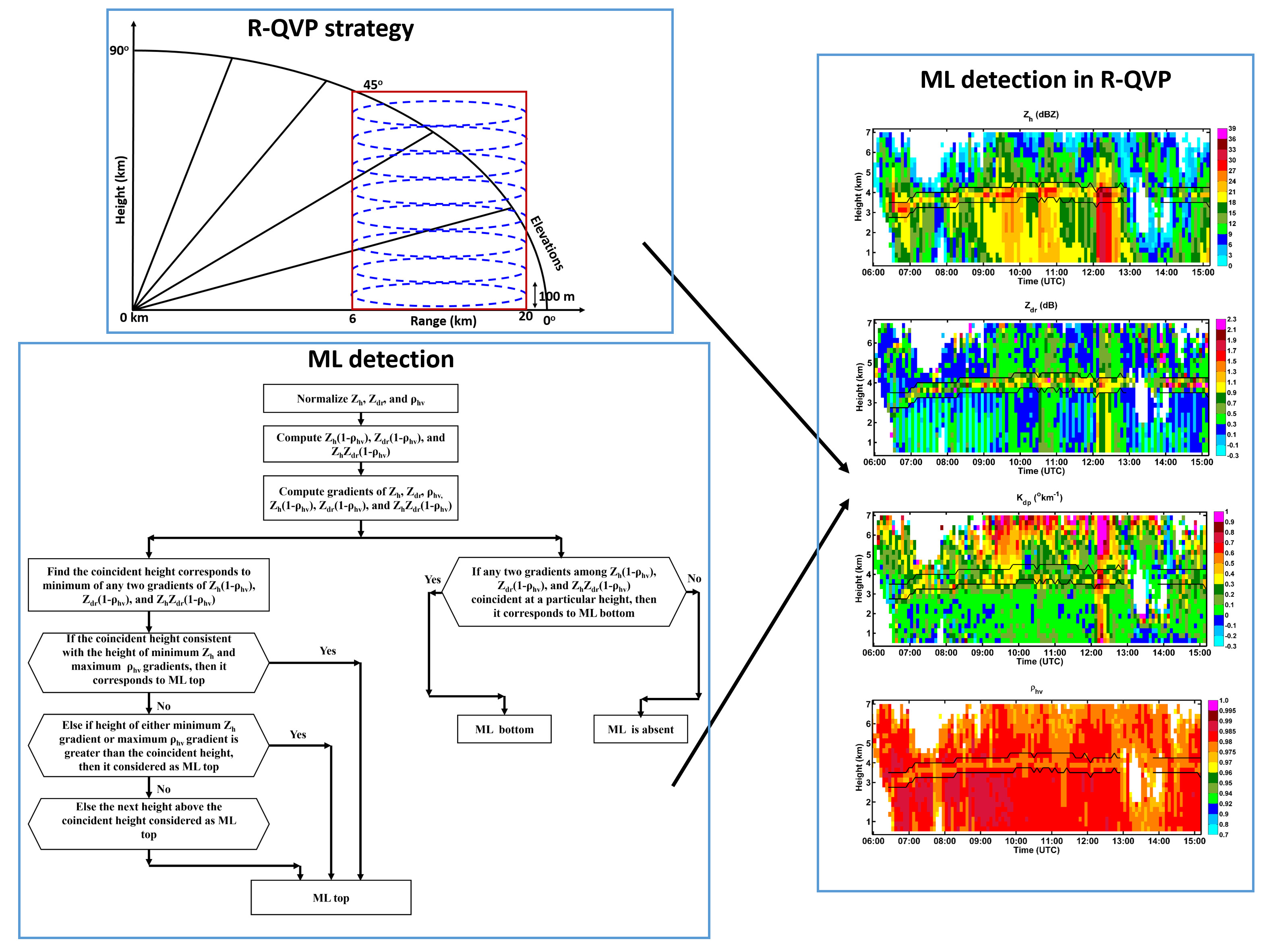
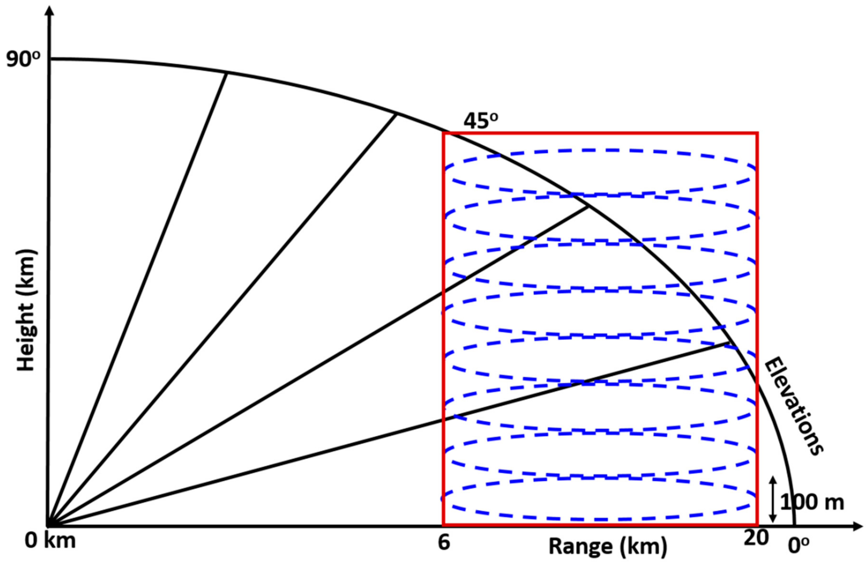
The R-QVP methodology is an efficient way to process and represent the RHI scans in the time–height form. This method provides the vertical structure of the precipitation event and temporal evolution of the storm. In this method, initially the range coordinate of the RHI data for a fixed azimuthal angle is converted/transformed into height (slant range converted into vertical height). Then, data from the multiple elevation angles within the 100 m grid spacing were averaged together. In the present study, we utilized the data which corresponded to ρhv > 0.6 and Zh ≥ 0 dBZ for the averaging process to reduce the non-meteorological contamination. The RHI data corresponding to the 109° azimuthal angle (Goyang region) were utilized for the averaging process. Further, we used data in the 6–20 km range and at low elevation angles (<45°) to reduce the ground clutter and beam broadening effects. The 100 m vertical and 5 min temporal resolutions were used in this strategy. The schematic diagram of the R-QVP strategy is shown in Figure 1. The R-QVP of Zh, Zdr, Kdp, and ρhv provided significant information related to the precipitation particle type and growth of the ice crystals. This method mitigated the errors and noise of the polarimetric radar variable. For more details of the R-QVP strategy the reader can refer to [15].
2.2. ML Detection Algorithm
The polarimetric variables, especially Zh, Zdr, and ρhv, are sensitive to the precipitation type, particle habits, and represent the ML characteristics. Therefore, we used a methodology based on Zh, Zdr, and ρhv, to detect the ML or BB. The Zh values increased in the ML owing to an increase in the dielectric factor of the particles, and possibly enhanced aggregation rates, before they melt into smaller raindrops and decrease in concentration because of flux divergence. The Zdr can easily exceed that of typical rain for pristine ice crystals, while snow aggregates tend to have Zdr below that of the equivalent rain distribution. In the ML, the ice particles transition to rain drops within the melting layer; hence, their axis ratio evolves during the particles change. Additionally, the raindrops are mostly aligned in the horizontal direction, and Zdr increases for smaller canting angles of raindrops compared to snow. The ML contains heterogeneous hydrometeors with various axis ratios of melting ice particles, raindrops, and wetted particles. Therefore, ρhv decreases in the ML. Wolfensberger et al. [6] proposed a gradient-based method for ML detection based on Zh and ρhv. However, for the ML detection, the Zdr and ρhv were important compared to Zh [2]. Furthermore, Zdr, ρhv, and Kdp, are more sensitive than Zh for precise ML detection [16] because of large and wetted particles presented in the ML. Thus, the Zh- and ρhv-based methods were unable to reliably detect the ML in some cases (when low ρhv and high Zh values present over the multiple height/range levels). Therefore, Zh, Zdr, and ρhv are robust descriptors of the shape, size, and type of the precipitation particles. Thus, in the present study, we refine the algorithm proposed by Wolfensberger et al. [6] and present a method based on Zh, Zdr, and ρhv and their combinations to detect reliably the ML. In this method, the values of Zh, Zdr, and ρhv were initially normalized by the maximum value in the respective profiles, and their gradients were then estimated. These gradients could not detect the true ML thickness in low ρhv and high Zh cases as described above. Therefore, the Zh and Zdr values were individually multiplied/combined with the complementary ρhv values, and the product of the Zh and Zdr values was multiplied with the complementary ρhv value that were used to describe the top and bottom ML parts. The combined parameters are shown below.
Zh·(1-ρhv)
Zdr·(1-ρhv)
Zh·Zdr·(1-ρhv)
Finally, the gradients were estimated for the absolute values of the normalized components of (1), (2), and (3). The corresponding heights of the maximum and minimum values of these gradients were then computed.
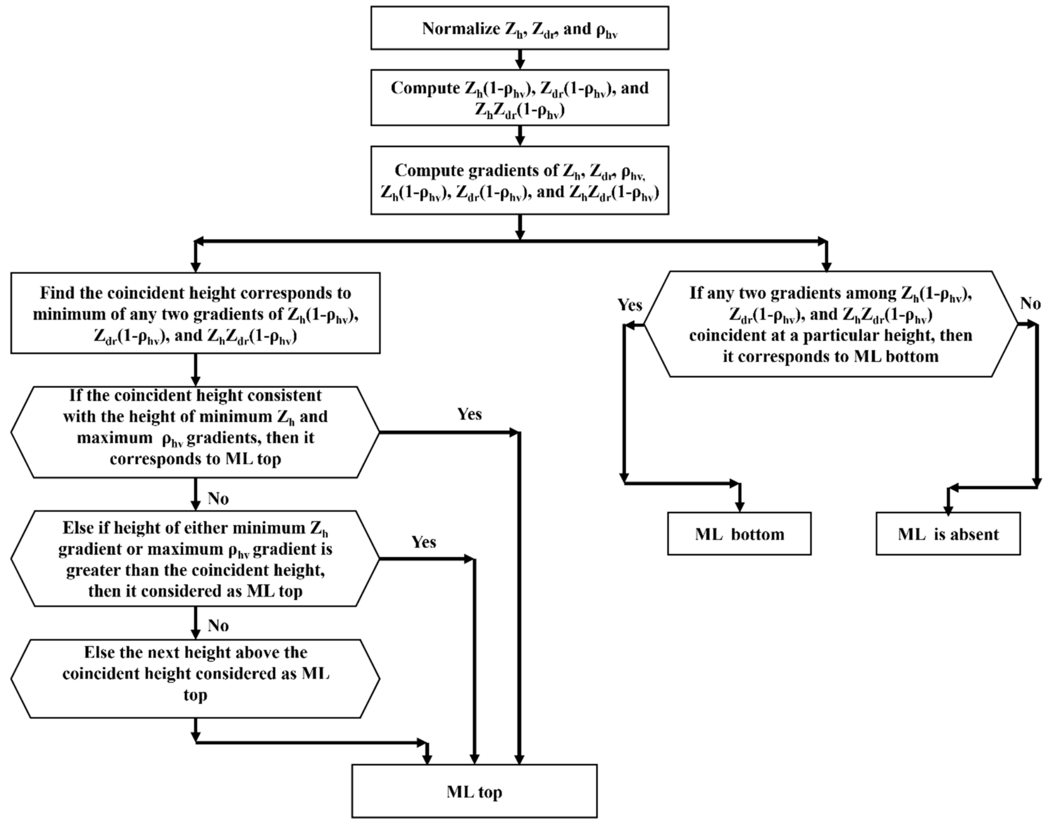
The ML boundaries were detected as follows:
Step 1. The coinciding height of the maximum values of any two gradients among (1), (2), and (3), represent the bottom part of the ML.
Step 2. The coinciding height corresponds to the minimum of any two gradients among (1), (2), and (3), and signifies the top ML part. However, in some cases, the Zdr peak is below the Zh peak and the ρhv minimum because the value of Zdr is low in ice and high in liquid. For this reason, the top part of the ML is associated with considerably high Zh and low ρhv values, while the bottom ML part is associated with increased Zdr values. Thus, the top part of the ML should be corrected.
Step 3. If the coinciding height presented in “Step 2” is consistent with the height of the minimum Zh and the maximum ρhv gradients, the corresponding height is then considered as the top part of the ML.
Step 4. If “Step 3” is not satisfied, the maximum height of either the height of the minimum Zh or maximum ρhv gradients should be greater than the coincident height (presented in “Step 2”). Correspondingly, this height represents the top part of the ML.
Step 5: If “Step 3” and “Step 4”are both unsuccessful, then the height above the coinciding height presented in “Step 2” is considered as the top part of the ML.
This method estimates the top and bottom parts of the ML efficiently. The flow chart of the proposed method is shown in Figure 2.
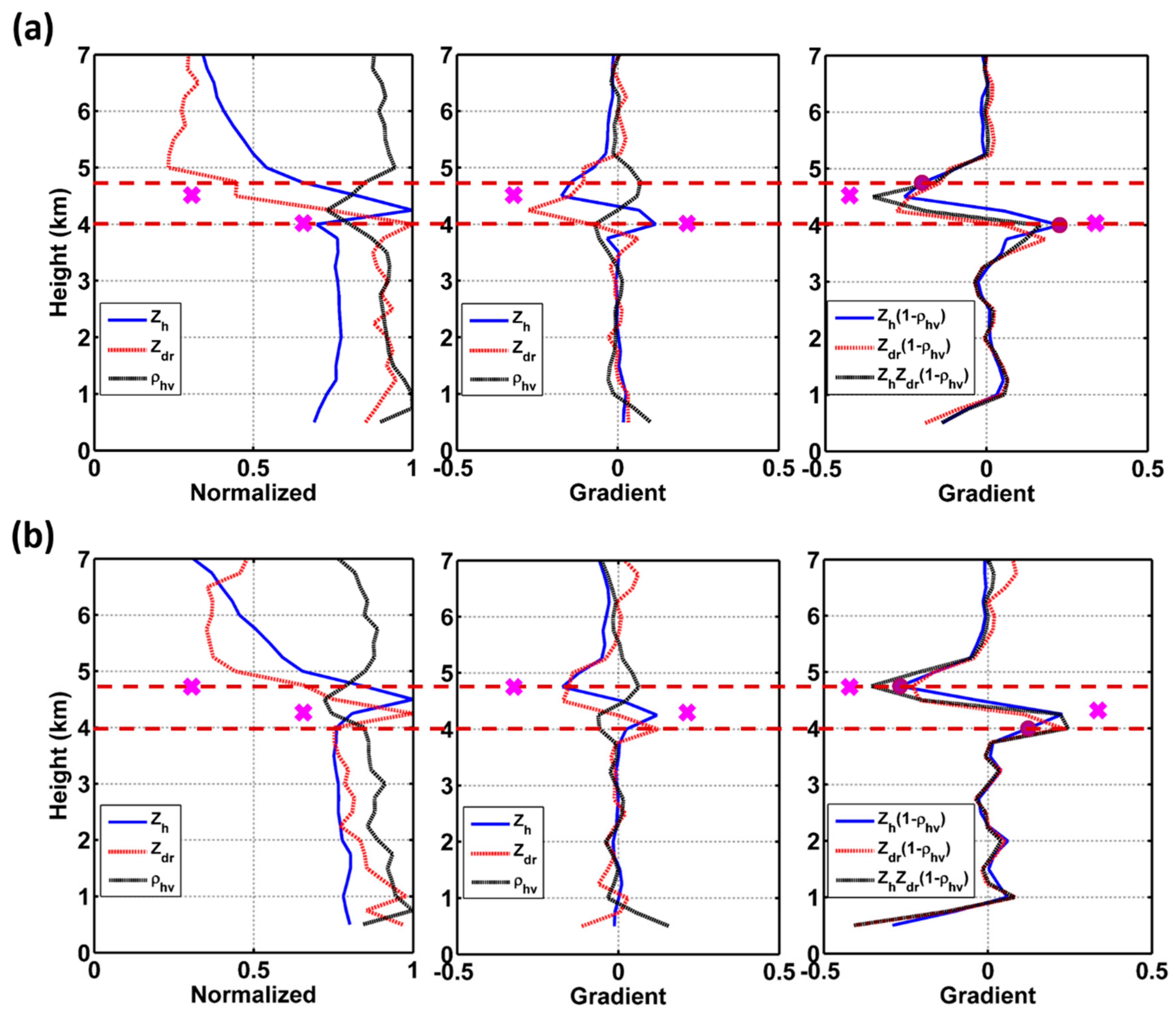
This algorithm was applied to the polarimetric variables, and the relevant example is shown in Figure 3. Figure 3a illustrates the profile obtained at 14:24 [coordinated universal time (UTC)] on 24 July 2014. The left panel represents the absolute normalized values (hereafter absolute normalized values are referred to as AN) of Zh (for simplicity referred to as AN(Zh)), Zdr (for simplicity referred to as AN(Zdr)), ρhv (for simplicity referred to as AN(ρhv)), and their gradients are illustrated in the middle panel. The gradients of AN of Zh(1-ρhv), AN of Zdr(1- ρhv), and AN of ZhZdr(1- ρhv), are shown in the right panel. The maxima of the gradient of AN(Zh(1-ρhv)) and the gradient of AN(ZhZdr(1-ρhv)) are coincident at 4 km. Thus, the 4-km height signifies the bottom of the ML. Similarly, the minima of the gradients of AN(Zh(1-ρhv)) and AN(ZhZdr(1-ρhv)) are coincident at a height of 4.5 km. However, the minimum and maximum gradients of Zh and ρhv are respectively presented at the different heights of 4.5 and 4.85 km. Therefore, the ML top represents the maximum height level of 4.85 km, which is presented above the coinciding height (4.5 km). The magenta color “x” marks represent the ML boundaries detected by the method based on Zh and ρhv [6], which shows that the bottom of the ML is similar to the proposed method. However, the top of the ML, at 4.5 km, differs from the current method. Figure 4c shows the height of the 0 °C wet-bulb temperature at 4.9 km, at 15:00 UTC (data extracted from MERRA; 14:30 UTC data not available). This example signifies that the proposed method estimates reliable ML boundaries.
Figure 3b corresponds to 14:34 UTC on 24 July 2014. The right panel shows that the gradients of AN(Zdr(1−ρhv)) and AN(ZhZdr (1−ρhv)) maxima are coincident at a height of 4 km, which signifies the bottom part of the ML. The minima of the gradients of AN(Zdr(1−ρhv)), AN(Zh(1−ρhv)), and AN(ZhZdr (1−ρhv)) are presented at a height of 4.85 km, and are also consistent with the minimum gradient of Zh and the maximum gradient of ρhv. Therefore, 4.85 km was designated as the top part of the ML. While, the Zh and ρhv gradient based method [6] illustrates the 4.25 km and 4.85 km boundaries (magenta “x”) of the ML. The top of the ML, at 4.85 km, is similar to the proposed method, whereas the bottom is different.
3. Observational Data and Processing
In this study, we used the data obtained from the X-band dual polarization radar operated by the Korea Institute of Civil Engineering and Building Technology (hereafter referred to as KICT radar), located approximately 20.6 km Northwest of Seoul, South Korea. The radar operates in the simultaneous transmission and reception mode at a frequency of 9.41 GHz. It provides one PPI and two RHI scans every minute, and a total of six PPI and 10 RHI scans in a 5 min period. The elevation angle of PPI alternates between 5° and 6°, while the RHI scans are produced every 18° in the azimuthal direction. The collected data incorporated the attenuation correction (ɸdp-based), data quality check [17], bias/error correction, and Kdp estimation [18] algorithms. For more details of the KICT radar location, the scanning strategy, and data quality control algorithms, the reader can refer to Chen et al. [19] and Allabakash et al. [15].
The atmospheric parameter data used in this study were collected from the MERRA and MERRA2 reanalysis datasets. The MERRA data was generated by the Global Modeling and Assimilation Office (GMAO) of the National Aeronautics and Space Administration (NASA) for the Goyang region using the Goddard Earth Observing System, version 5 (GEOS-5), data assimilation system [20]. The MERRA2 reanalysis data were also produced by the NASA GMAO with the use of the GEOS-5.12.4 system [21]. We used MERRA and MERRA-2 for vertical/spatial and horizontal/temporal data, respectively. The vertical profiles of wet-bulb temperature, RH, cloud liquid water mixing ratio (QL), and cloud ice mixing ratio (QI), and the surface/horizontal profiles of T, RH, precipitation (P), and horizontal wind speed (WS) were derived for the Goyang Province.
4. Results and Discussion
4.1. Case 1: 24 July 2014
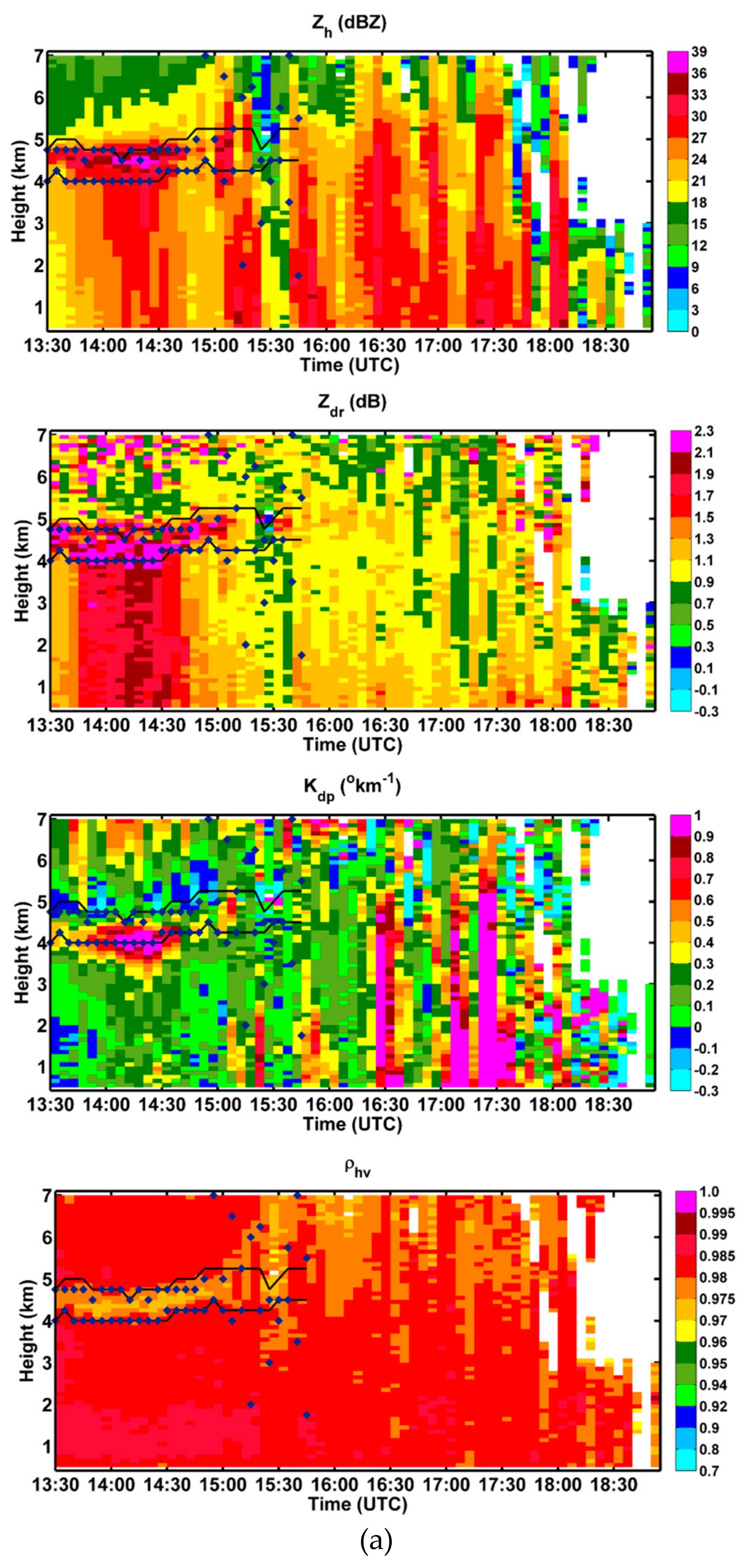
On 24 July 2014, a precipitation event occurred in the Goyang region. The polarimetric radar signatures defined the structure of this event. The R-QVP profiles provided the spatial and temporal error mitigated polarimetric variables. Figure 4a shows the R-QVP vertical profiles of the Zh, Zdr, Kdp, and ρhv corresponding to this event. The ML was estimated using the method described above and illustrated as black solid lines. On the other hand, the diamond markers indicate the ML estimated using the gradients of Zh and ρhv values [6]. The upper and lower solid/marker lines indicate the top and bottom parts of the ML, respectively. It can be noted that at 14:15 and 15:15 UTC, ρhv was greater
than 0.98. Accordingly, it was difficult to identify the top and bottom parts of the ML using Zh and ρhv, and the markers (Zh and ρhv based method) showing unstable high/low values are not reliable. However, the combination of the Zh and Zdr values in conjunction with the values of ρhv wa3s more useful in these cases. The solid lines (proposed method) show the reliable and stable ML boundaries. It is clearly observed that low ρhv values (< 0.98), high Zh values (≥ 28 dBZ), and high Zdr values (≥ 1.5 dB) are obtained in the ML. Furthermore, the ML also contains high Kdp values (> 0.5° km−1).
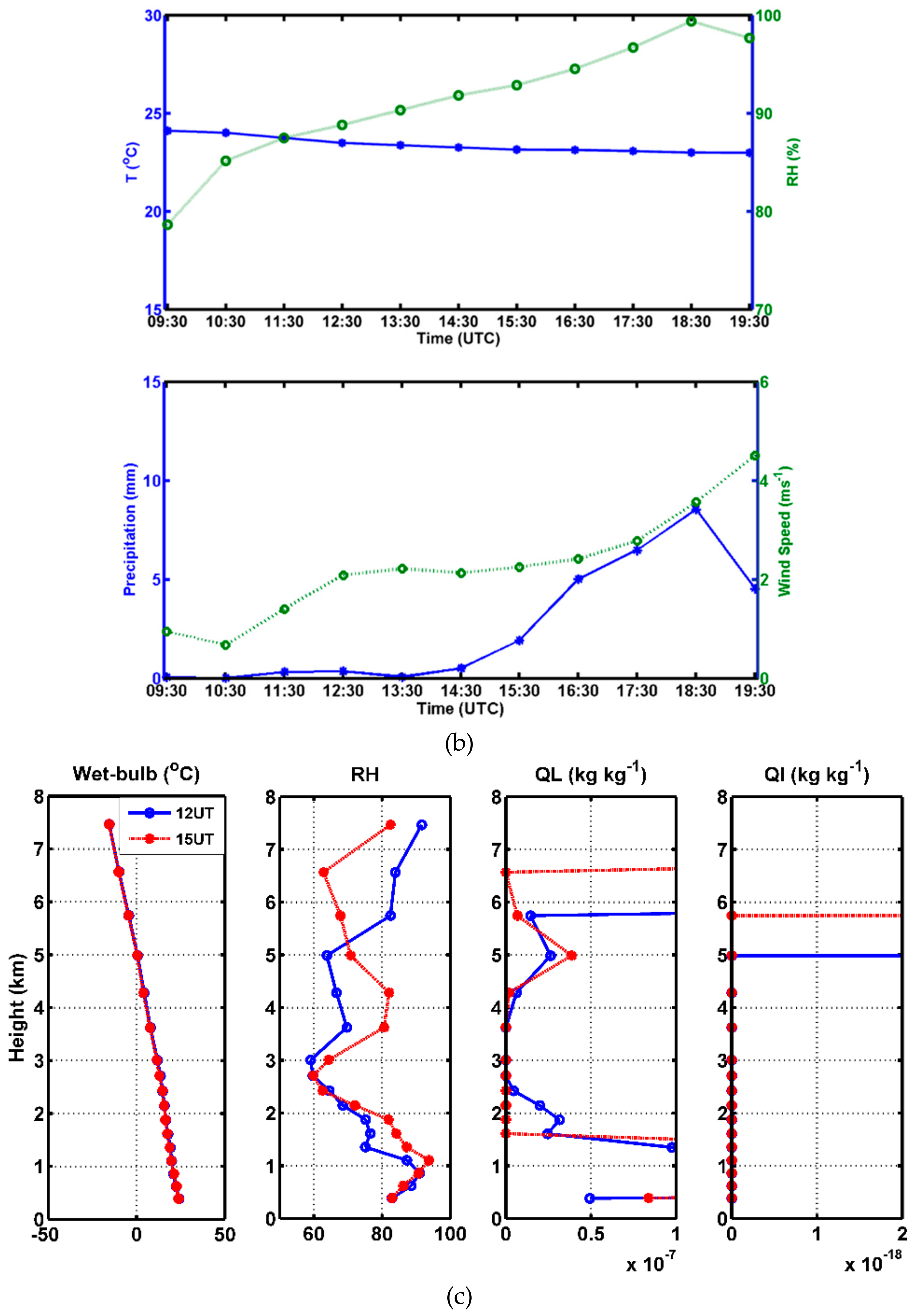
To describe and verify the ML structure, the surface parameters of T, RH, P, and WS, and the vertical parameters of wet-bulb temperature, RH, QL, and QI were extracted from MERRA2/MERRA and are illustrated in Figure 4b,c, respectively. T decreases and RH increases from 13:30 UTC onward, as shown in Figure 4b. Furthermore, RH increases above 90%, which was conducive to rainfall. Correspondingly, the precipitation exhibits increasing trend. The vertical profiles show the corresponding height of the ML. The 0 °C wet-bulb temperature at a height of 4.9 km, corresponds to the top part of the ML. Furthermore, RH values increased for heights in the range, 3.5 to 5 km. The LWC (represented by QL) and the IWC (represented by QI) yield maximum values for heights in the range from 4 to 5 km, thus signifying the mixing of the liquid and solid (ice) particles in the ML. Thus, based on this analysis, we infer that the proposed algorithm was reliable in detecting the true ML. Figure 3a and Figure 4a show that the Zdr peak is always present below the Zh peak. The Zdr peak was present at lower heights and at T > 0 °C. Therefore, the melting of the hydrometeors led to a Zdr maximum occurs at lower height levels than the Zh peak. Thus, this offset signifies the maximum eccentricity of the melting particles [16]. Further, at lower level of the ML, the smallest particles had already collapsed into nearly spherical raindrops that were small and contributed less to Zh, leaving the largest aggregates dominating Zh and thus occur Zdr magnitude.
4.2. Case 2: 11 May 2015
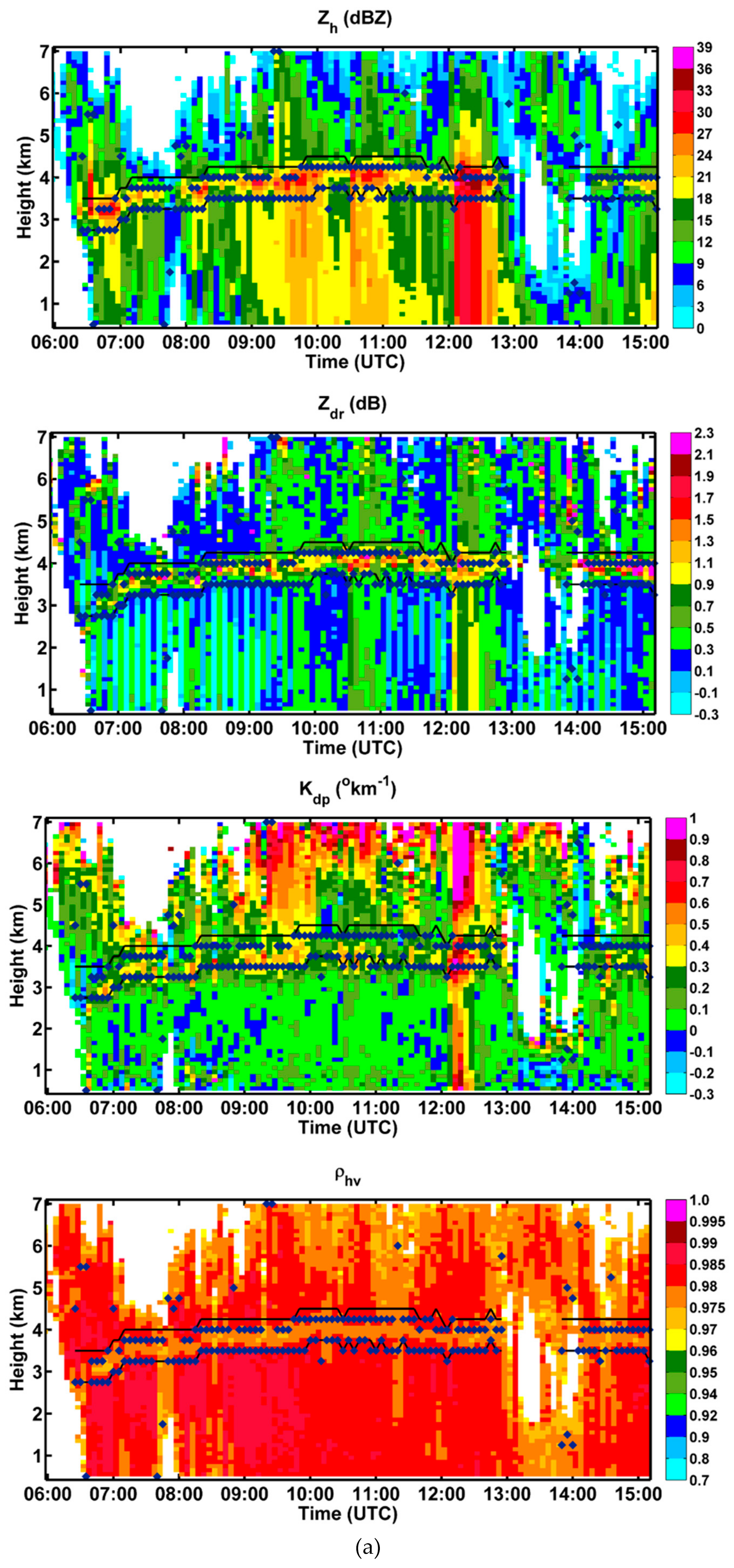
The R-QVP profiles related to this event are shown in Figure 5a. The solid lines (proposed method) show the stable ML boundaries, while the markers (based on Zh and ρhv) show unstable ML thickness. The top of the ML estimated using the current method is consistent with the 0 °C wet-bulb temperature (shown below). The ML boundaries can be observed for heights in the range of 3–4 km. The thickness of the ML was approximately 0.7 km. If there was an abrupt change in the ML thickness, then the top and bottom parts of the ML were interpolated with their adjacent values. Alternatively, it was considered that BB was absent. It can be observed that from 13:00 to 14:00 UTC, the BB was absent. The ML contains increased Zh, Zdr, and Kdp values with decreased ρhv values that illustrate the different hydrometeors types. The increased Kdp values in the ML indicate the large melting aggregates of ice particles. Intriguing signatures can be observed in Figure 5a. The Zh is higher on the bottom side of the BB (>15 dBZ) than the top (≤15 dBZ), and represent rain and ice, respectively [22]. Conversely, the Kdp trend was opposite in the cases of Zh and Zdr (above and below of ML). Correspondingly, the Kdp values increased for solid particles and decreased for liquid particles. Furthermore, slightly depressed ρhv values were present above ML owing to depositional growth of the pristine ice crystals [23]. It is interesting to note that the Kdp value increased from 09:00 to 13:00 UTC at the cloud top temperature (−20 °C) associated with the moderate Zdr values, thus signifying the large concentration of isometric particles [9,15].
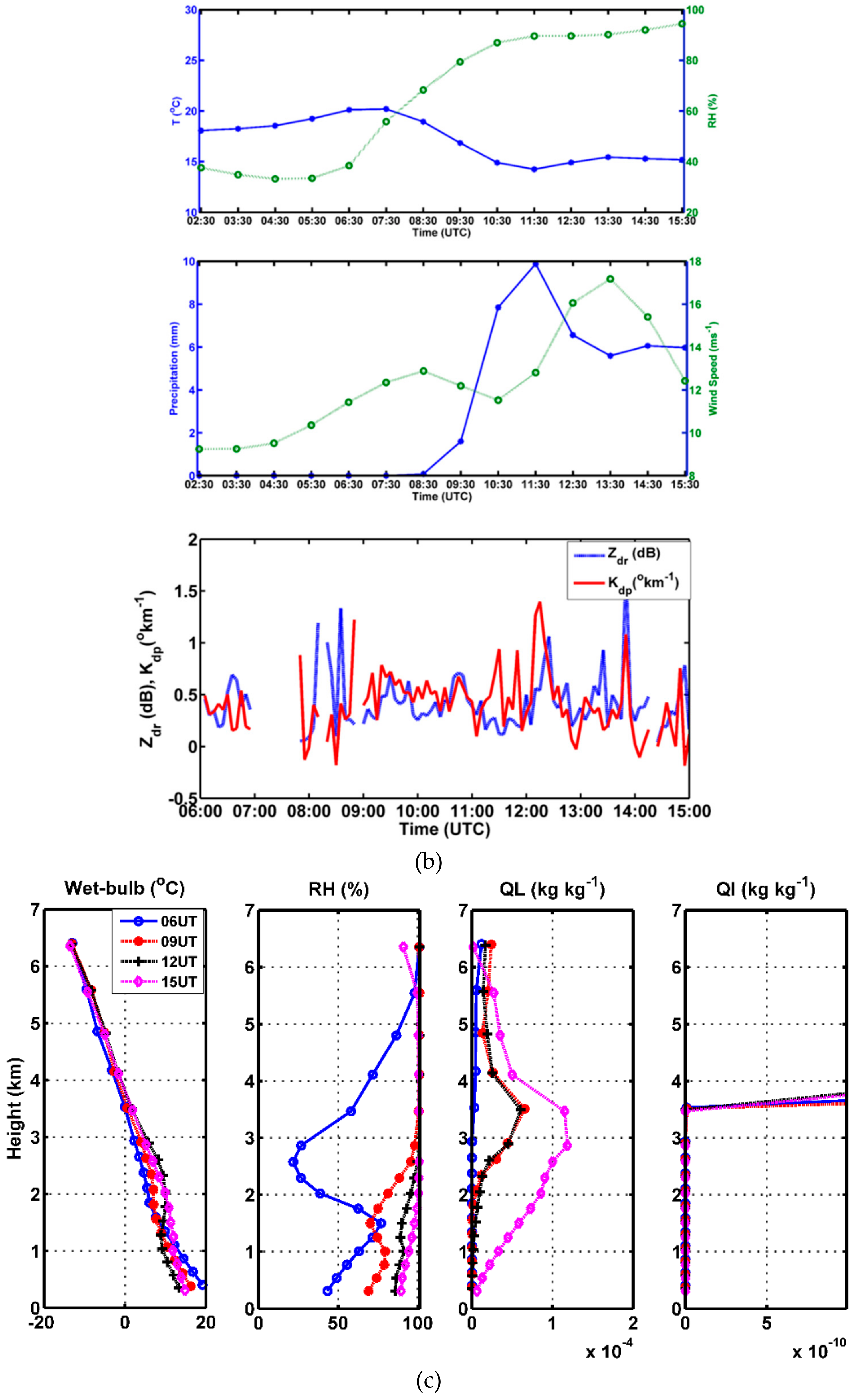
The corresponding surface parameters are shown in Figure 5b. The respective decreasing and increasing T and RH trends from 06:30 UTC signify the formation of precipitation. The enhancement of precipitation and WS can also be observed in Figure 5b. It is interesting to note the high precipitation at/followed by the high Zdr and Kdp values present in the dendritic growth layer (DGL) between the temperature range, −10 to −15 °C [15,23,24]. The Zdr and Kdp values between −10 and −15 oC were averaged for each height and presented in the bottom panel of Figure 5b. The high Zdr and high Kdp presented at 08:00–09:00 UTC, and precipitation also started during this period (see middle panel of Figure 5b). Again, the enhanced Zdr and Kdp values occurred at 11:00–13:00 UTC, where high precipitation was observed on the ground. The vertical profiles of the meteorological parameters are shown in Figure 5c. The plot of wet-bulb temperature shows the 0 °C isotherm in the range of 3.5–3.8 km at different times that correlates with the ML heights. It is interesting to note that the LWC and IWC show enhanced values at the ML boundary in the range of 3–4 km and illustrate the mixed phase hydrometeors. At 06:00 UTC, P and ML had small amplitudes, but had increased amplitudes at 09:00, 12:00, and 15:00 UTC. Correspondingly both QL and RH also showed low values at 06:00 UTC and high values (100%) at other times.
4.3. Case 3: 2 December 2015
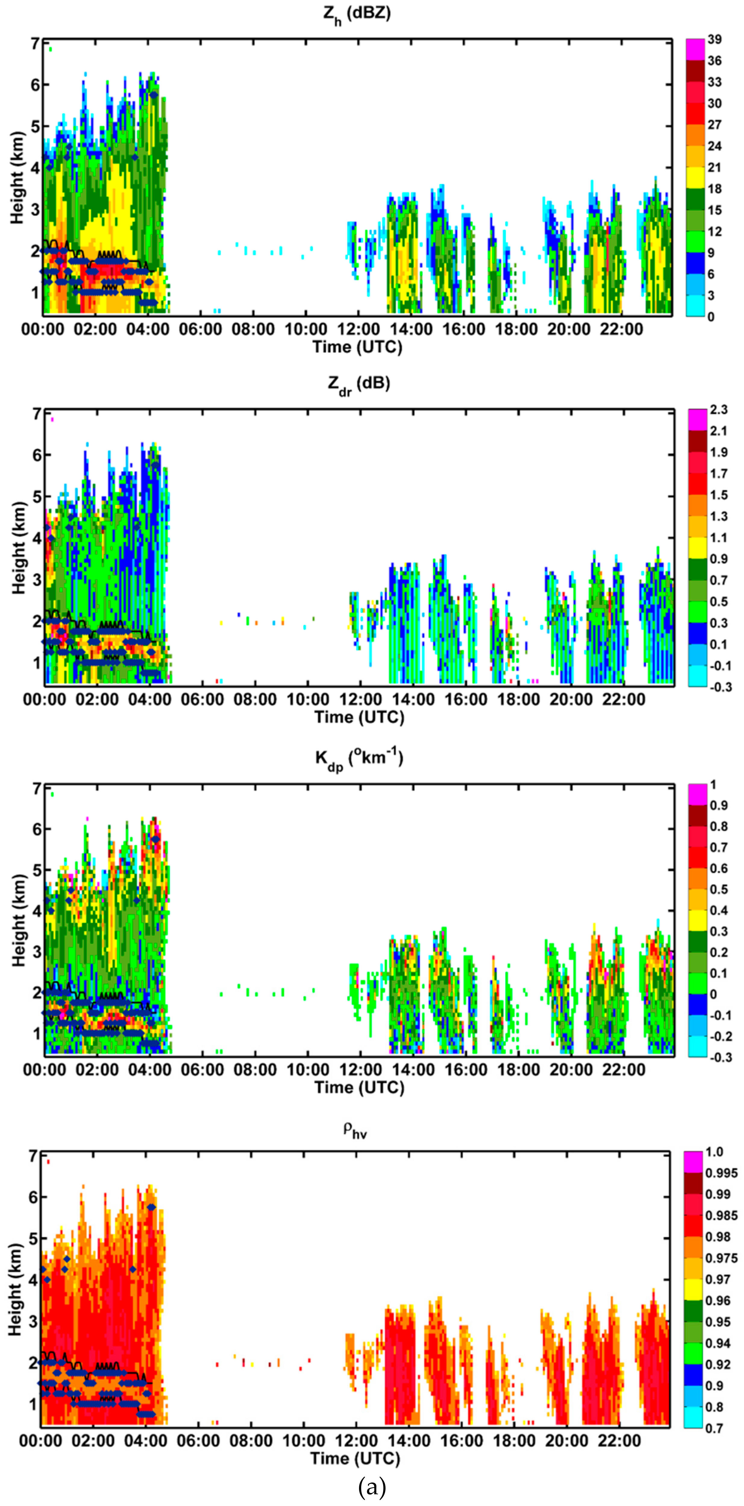
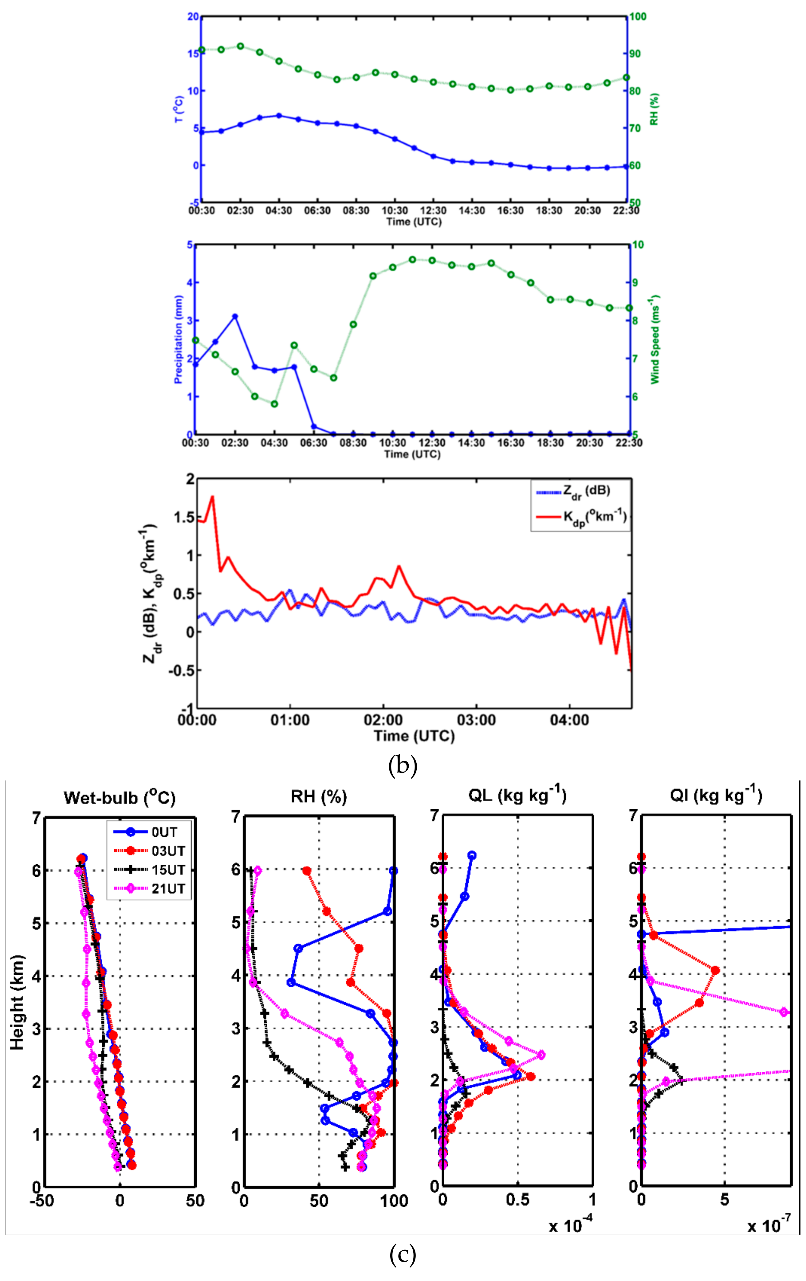
This case corresponds to a winter precipitation event. The R-QVP profiles are illustrated in Figure 6a and the corresponding surface and vertical parameters are shown in Figure 6b,c, respectively. Figure 6a clearly shows the proposed method (solid lines) evaluated a reliable ML, in contrast to the Zh and ρhv based method (diamond markers). The ML shows significant polarimetric signatures. In the winter, the top and bottom parts of the ML are present at lower heights in the range of 1–2 km. It is clearly shown that the solid phase particles exhibit low Zh, low Zdr, high Kdp, and low ρhv values, while the opposite is true for rain hydrometeors.
The surface parameters (Figure 6b) exhibit increased RH values from 00:00 to 04:00 UTC, while the surface precipitation is also shown to be greater than 1 mm on the ground. The averaged Zdr and Kdp values of DGL are shown in Figure 6b bottom panel. In DGL, at some instances high Kdp was present without high Zdr [25]. The averaged Kdp values of DGL are shown at 00:00–01:00 UTC and at 02:00–2:30 UTC, and high precipitation was also observed during this time, especially during the later time period. The vertical wet-bulb temperature (Figure 6c) illustrates the 0 °C isotherm at a height of 2 km, which corroborates the ML findings. Furthermore, the RH was enhanced (100%), while the QL and QI were also high in the 1–4 km height range and represent the liquid and ice hydrometeors. From 12:00 UTC onward, rainfall changed over to snowfall owing to the negative temperatures, as observed by the surface T values.
4.4. Case 4: 5 March 2016
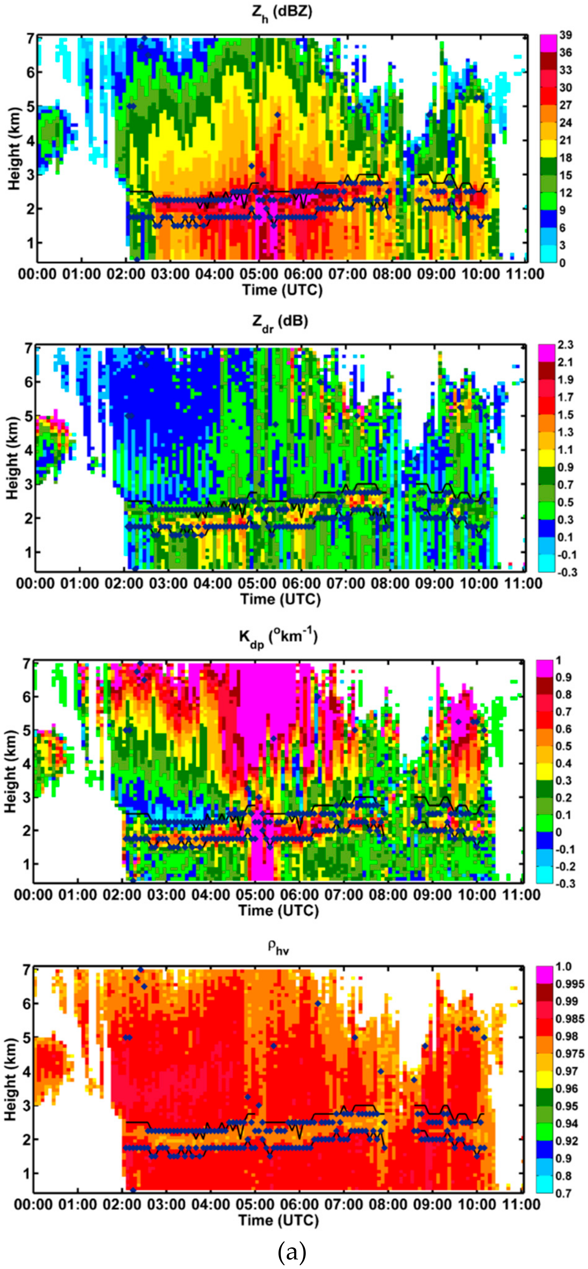
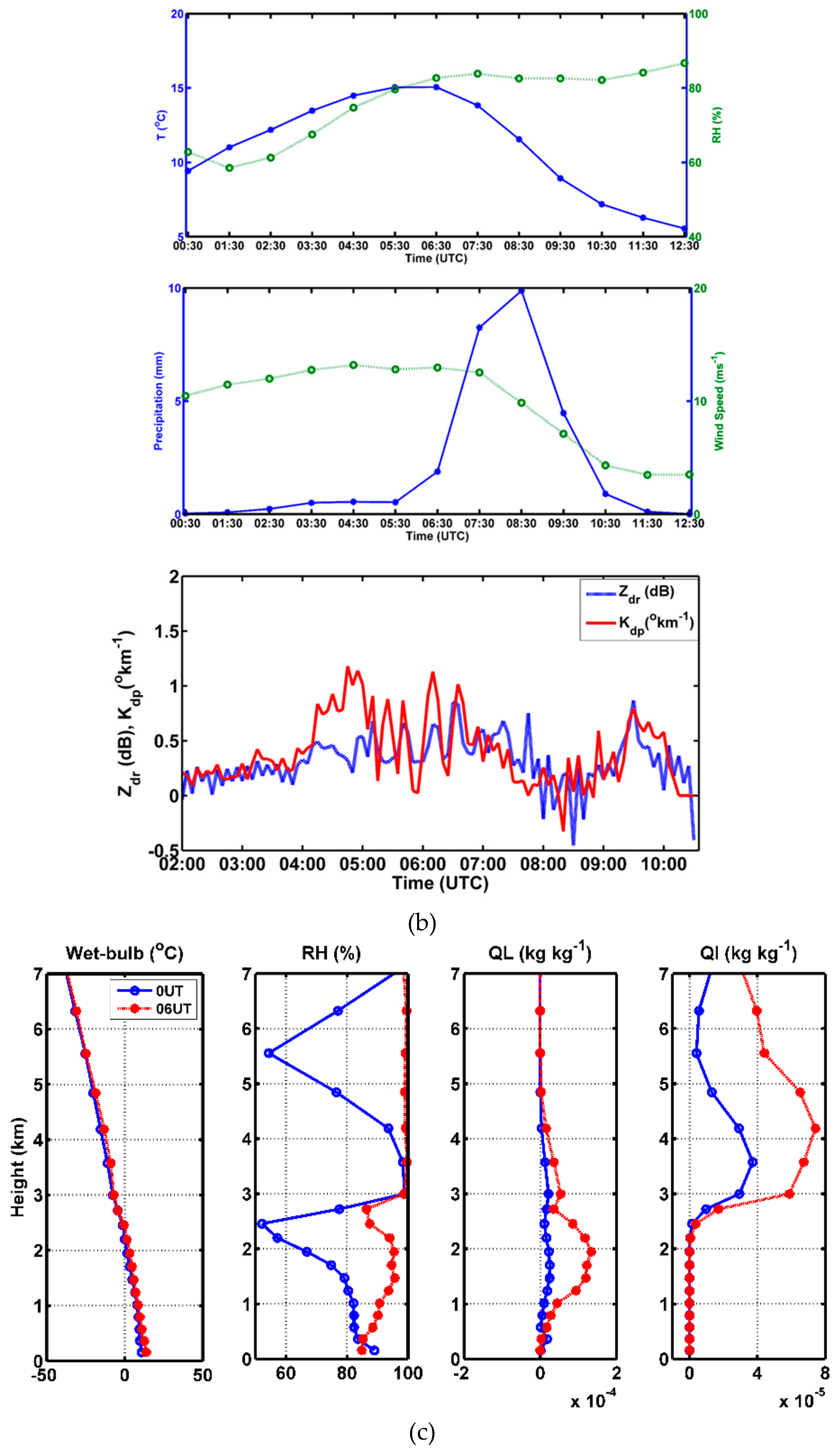
Figure 7a shows the R-QVP profiles of polarimetric variables corresponding to this event. The solid lines (proposed method) show smooth/reliable ML boundaries, in contrast to the diamond markers (Zh and ρhv based method). The ML can be observed within the 1.5–2.8 km height range. The surface and vertical parameters are illustrated in Figure 7b,c, respectively. From 02:00 UTC onward, the RH increases that indicates the rain falling into a dry layer near the surface. The surface precipitation also shows an increasing trend from 02:00 UTC onward. The enhanced Zdr and Kdp of DGL (bottom panel) shown at 03:30–07:00 UTC illustrates the start of the precipitation (see middle panel). Again, high values are presented at 08:30–10:00 UTC, signifying heavy precipitation on the ground. The vertical wet-bulb temperature illustrates the 0 °C isotherm at an approximate height of 2 km, whereby the QL and QI also show enhanced values for heights in the range from 2–4 km, while RH values greater than 80% refer to mixed precipitation particles in the ML.
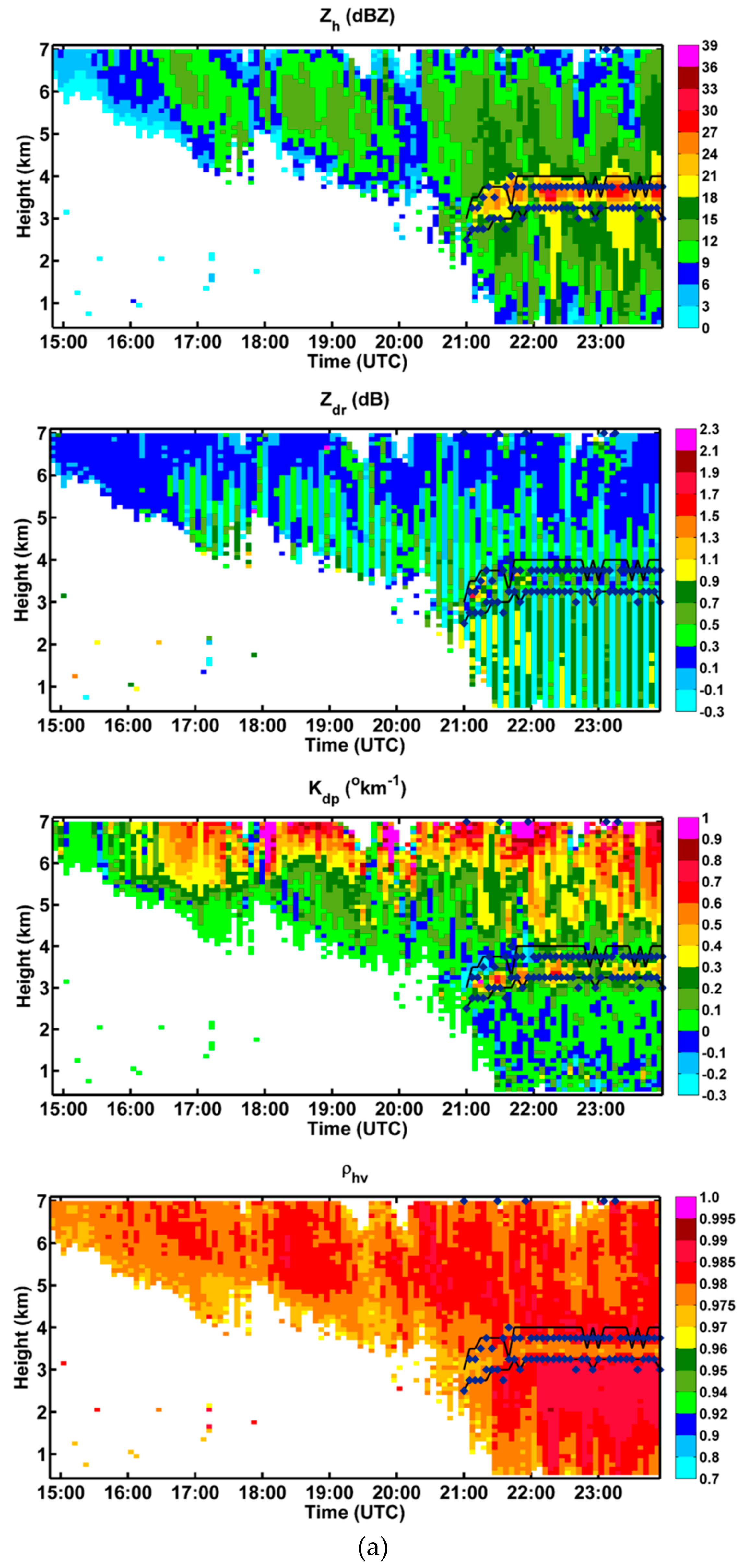
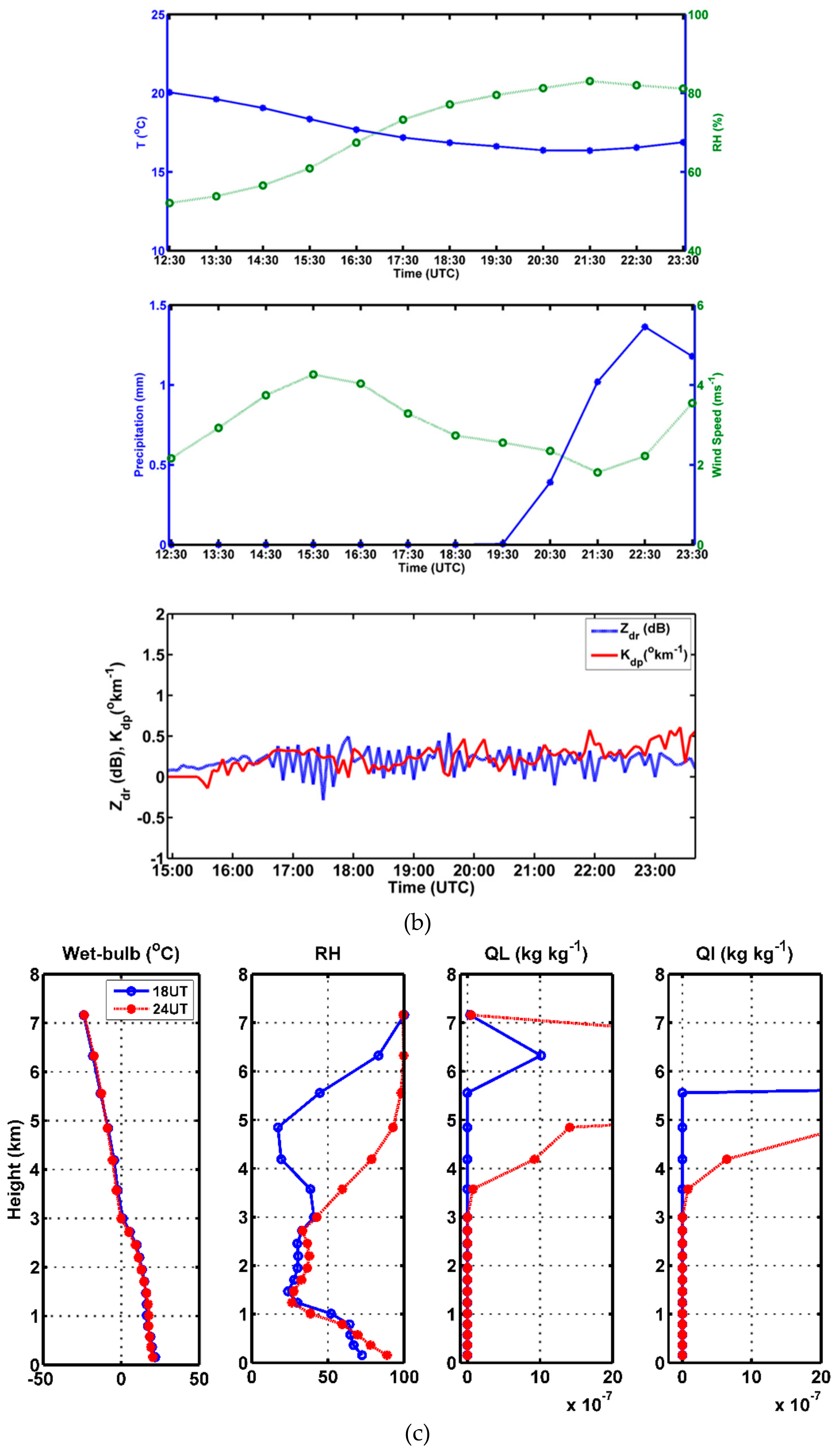
4.5. Case 5: 1 October 2016
In this case, the proposed method (solid lines) signifies the true ML boundaries, while the diamond markers (Zh and ρhv based method) show uncertain ML values, as shown in Figure 8a. The ML was observed at heights in the range of 2.5–3.5 km. The RH and surface precipitation also exhibit higher values from 19:30 to 23:30 UTC (Figure 8b), and also high Kdp of DGL also observed during this interval, especially at 21:00–23:30 UTC time period (where high precipitation presented). The wet-bulb temperature shows 0 °C isotherm at 3.2 km height. The enhanced signatures of the vertical parameters of the RH, QL, and QI, are presented for heights in the range of 3–4 km, which correspond to the ML height.
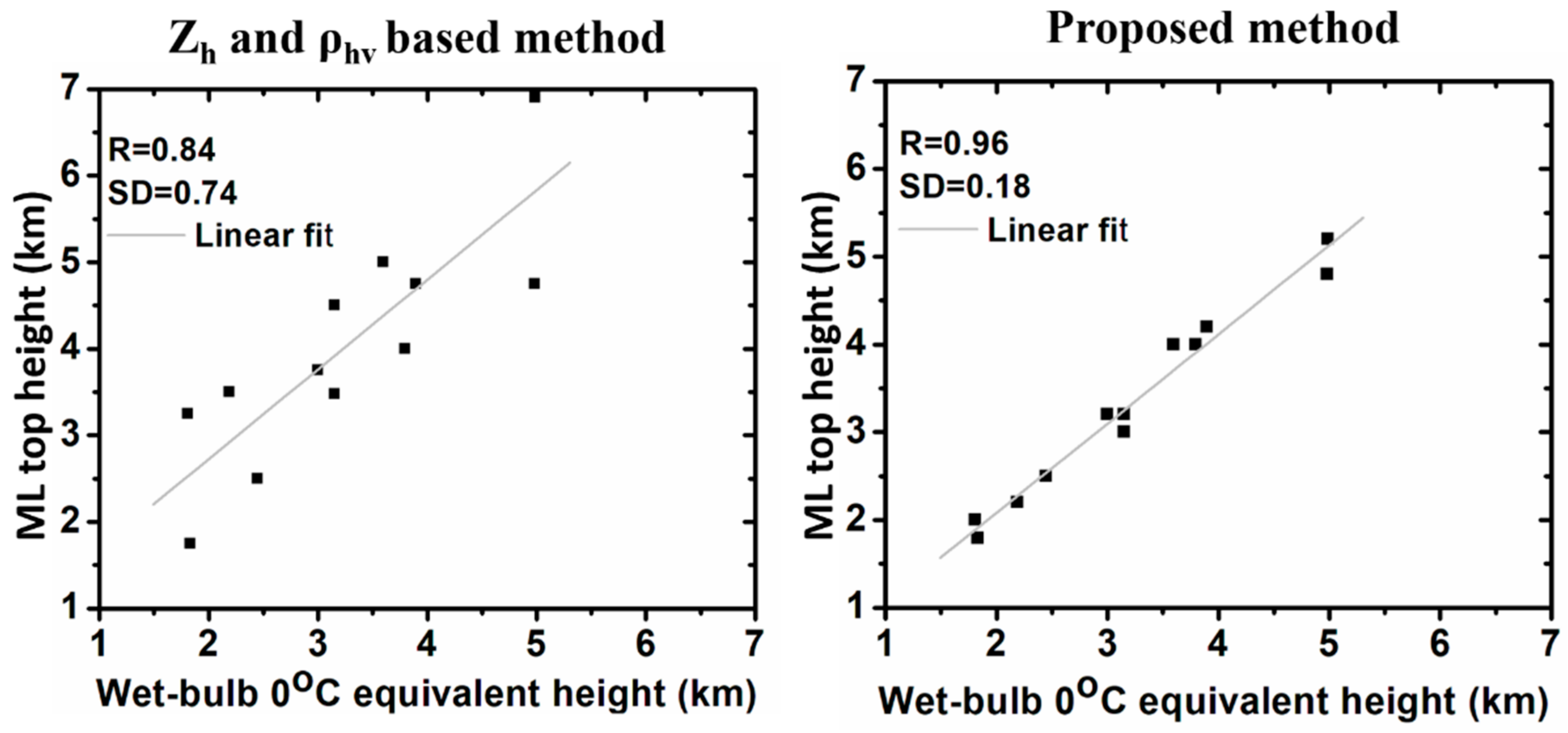
The ML heights obtained from the Zh and ρhv-based methods and the proposed method for all the cases were compared with the wet-bulb 0 °C isotherm and presented as a scatter plot, shown in Figure 9. The figure shows that the proposed method produced high correlation (0.96) with lower standard deviation than that of the Zh and ρhv-based method (correlation = 0.84, standard deviation = 0.18). Thus, we advocate that the current method is efficient at ML estimation.
5. Polarimetric Variables Statistics in ML, Rain, and Snow
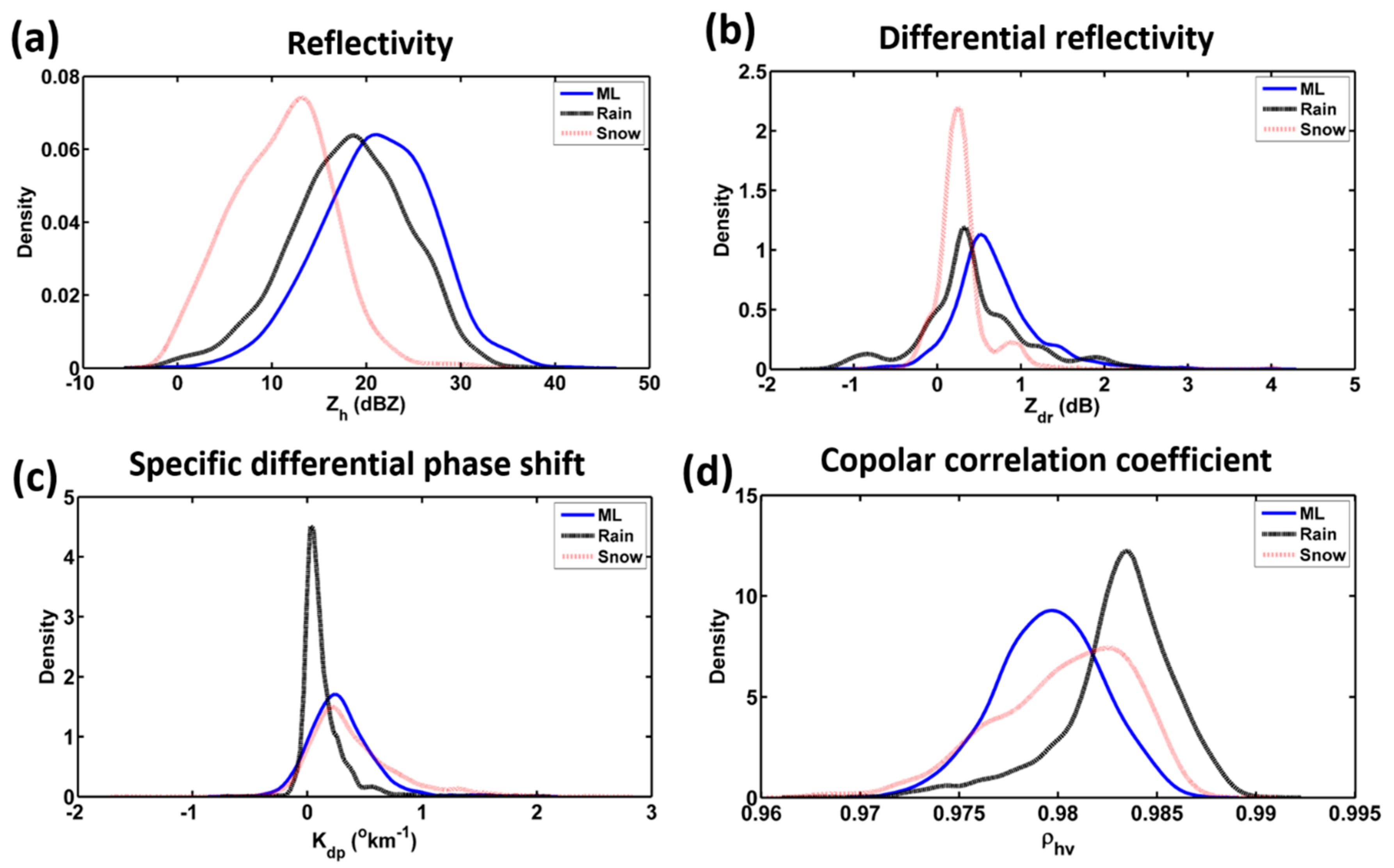
Based on the above case studies, we evaluated the statistics of Zh, Zdr, Kdp, and ρhv in the ML, rain, and snow. The distributions of these variables are shown in Figure 10 and their statistics in different quantiles are presented in Table 2. Zh in the ML shows symmetrical distributions with a mean value of 21 dBZ. The quantile 10 (Q10), Q50, and Q90 values are 13.23, 21.15, and 28.38, respectively. Zh in rain is more symmetrical than that of Zh in snow and the ML. Zh in snow contains lower values and is left-skewed. Zdr in the ML shows a right-skewed distribution with a mean value of 0.69. Zdr in rain and snow shows similar distributions to Zh. In the ML, ρhv shows symmetrical distributions and the values are contained in a small area with a mean of 0.978. The ρhv values within the ML is lower than in the liquid and solid phase particles. The ρhv values in rain is right skewed with higher values than that of ρhv in the ML and snow. The distributions of Zh, Zdr, and ρhv are similar to the results presented by [1] and [6]. Kdp in the ML exhibits left skewed distributions with a mean of 0.29. Kdp in snow and the ML exhibit similar distributions, but the Kdp spread in snow is slightly larger than in the ML. The phase of the particles were easily described by these distributions. From all the distributions and statistics shown in Table 2, we infer the following:
- The enhanced values of Zh, Zdr, and Kdp, and low ρhv values present in the ML are due to the mixed phase of hydrometeors.
- Zh is lower in the snow region than in rain due to lower dielectric effects of ice particle [26].
- The snow aggregates are larger with low density and randomly oriented, producing smaller Zdr (< 0.5 dB) values in the snow than in rain [15].
- ρhv is lower in pristine ice crystals, especially mixed with aggregates [26], thus the snow region contains a lower ρhv than that of the rain region.
It is known that the ML varies according to the seasons owing to the variability of the 0 °C isotherm. We also observed this feature. The top and bottom parts of the ML were high in the summer, followed by autumn, spring. Additionally, it is shown that ML is low in winter. We also observed that the thickness is independent of the season and the spatial location within this region. Table 3 shows the boundaries of the ML during different seasons.
6. Summary and Conclusions
In this study, we proposed a new and refined simple automatic method to detect the ML thickness based on R-QVPs of polarimetric variables. The algorithm utilized X-band dual polarization radar data obtained in South Korea. The gradients of Zh, Zdr, ρhv, Zh(1-ρhv), Zdr(1-ρhv), and ZhZdr(1-ρhv), were used to describe the top and bottom parts of the ML. The enhanced values of Zh, Zdr, Kdp, and depressed ρhv in the ML were indicative of the heterogeneous hydrometeors. The low values of Zh, Zdr, ρhv, and high values of Kdp present on top of the ML indicated the solid phase of the precipitation particles. Conversely, the Zh, Zdr, ρhv values were high and the Kdp values were low below the ML, thus signifying the liquid phase of the hydrometeors. The Zdr peak present below the Zh peak in the ML was attributed to the eccentricity of the hydrometeors. The R-QVP profiles presented the error mitigated polarimetric variables that exhibited spatial and temporal variabilities of the ML signatures. The ML was high in the summer followed by the autumn, spring, and winter, owing to the variability of the height of the 0 °C isotherm. The ML thickness was independent of the season and the spatial location within this region. The detected ML was also verified by the wet-bulb temperature profile derived from the MERRA reanalysis data. The ML was mostly associated with the enhanced values of RH, QL, and QI. The increased values of QL and QI in the ML signified a mixed hydrometeor phase (liquid and solid). The distributions and statistics of the polarimetric variables in the ML, rain, and snow regions signified the phase of the hydrometeors in these regions. We also observed high Zdr and Kdp values in DGL, indicative of high precipitation on the ground, similar to the observations of Trömel et al. [29].
The ML detection in the R-QVP profiles is useful for the QPE estimation and hydrometeor classification algorithms than the conventional ML detection methods based on PPI/ RHI scans. These are particularly important to identify the particle types in the precipitation events for aviation forecasting. The combined methodologies of Allabakash et al. [15] and this method are useful for forecasting the heavy rain/QPE and snowfall, and provide early warnings to the public.
Author Contributions
Conceptualization, S.A. and S.L.; formal analysis, S.A. and S.L.; writing—original draft, S.A.; writing—review and editing, S.L. and B.-J.J.
Funding
This work was supported by the Korea Institute of Civil Engineering and Building Technology Strategic Research Project (Development of Driving Environment Observation, Prediction and Safety Technology Based on Automotive Sensors).
Acknowledgments
The authors would also like to thank MERRA and MERRA2 for providing the different datasets used in this paper.
Conflicts of Interest
The authors declare no conflict of interest.
References
- Giangrande, S.E.; Krause, J.M.; Ryzhkov, A.V. Automatic designation of the melting layer with a polarimetric prototype of the WSR-88D radar. J. Appl. Meteorol. Climatol. 2008, 47, 1354–1364. [Google Scholar] [CrossRef]
- Boodoo, S.; Hudak, D.; Donaldson, N.; Leduc, M. Application of dual-polarization radar melting-layer detection algorithm. J. Appl. Meteorol. Climatol. 2010, 49, 1779–1793. [Google Scholar] [CrossRef]
- Matrosov, S.Y.; Clark, K.A.; Kingsmill, D.E. A polarimetric radar approach to identify rain, melting-layer, and snow regions for applying corrections to vertical profiles of reflectivity. J. Appl. Meteorol. Climatol. 2007, 46, 154–166. [Google Scholar] [CrossRef]
- Shusse, Y.; Maesaka, T.; Kieda, K.; Iwanami, K. Polarimetric radar observation of the melting layer in a winter precipitation system associated with a South-coast cyclone in Japan. J. Meteorol. Soc. Jpn. Ser. II 2019, 97, 375–385. [Google Scholar] [CrossRef]
- Yuan, F.; Lee, Y.; Meng, Y.; Ong, J. Characterization of S-band dual-polarized radar data for the convective rain melting layer detection in a tropical region. Remote Sens. 2018, 10, 1740. [Google Scholar] [CrossRef]
- Wolfensberger, D.; Scipion, D.; Berne, A. Detection and characterization of the melting layer based on polarimetric radar scans. Q. J. R. Meteorol. Soc. 2016, 142, 108–124. [Google Scholar] [CrossRef]
- Van den Heuvel, F.; Gabella, M.; Germann, U.; Berne, A. Characterisation of the melting layer variability in an Alpine valley based on polarimetric X-band radar scans. Atmos. Meas. Tech. 2018, 11, 5181. [Google Scholar] [CrossRef]
- Ryzhkov, A.; Zhang, P.; Reeves, H.; Kumjian, M.; Tschallener, T.; Trömel, S.; Simmer, C. Quasi-vertical profiles—A new way to look at polarimetric radar data. J. Atmos. Ocean. Technol. 2016, 33, 551–562. [Google Scholar] [CrossRef]
- Griffin, E.M.; Schuur, T.J.; Ryzhkov, A.V. A polarimetric analysis of ice microphysical processes in snow, using quasi-vertical profiles. J. Appl. Meteorol. Climatol. 2018, 57, 31–50. [Google Scholar] [CrossRef]
- Tobin, D.M.; Kumjian, M.R. Polarimetric radar and surface-based precipitation-type observations of ice pellet to freezing rain transitions. Weather. Forecast. 2017, 32, 2065–2082. [Google Scholar] [CrossRef]
- Kumjian, M.R.; Mishra, S.; Giangrande, S.E.; Toto, T.; Ryzhkov, A.V.; Bansemer, A. Polarimetric radar and aircraft observations of saggy bright bands during MC3E. J. Geophys. Res. Atmos. 2016, 121, 3584–3607. [Google Scholar] [CrossRef]
- Kaltenboeck, R.; Ryzhkov, A. A freezing rain storm explored with a C-band polarimetric weather radar using the QVP methodology. Meteorol. Z. 2017, 26, 207–222. [Google Scholar] [CrossRef]
- Bukovčić, P.; Zrnić, D.; Zhang, G. Winter precipitation liquid–ice phase transitions revealed with polarimetric radar and 2DVD observations in central Oklahoma. J. Appl. Meteorol. Climatol. 2017, 56, 1345–1363. [Google Scholar] [CrossRef]
- Kumjian, M.R.; Lombardo, K.A. Insights into the evolving microphysical and kinematic structure of northeastern US winter storms from dual-polarization Doppler radar. Mon. Weather. Rev. 2017, 145, 1033–1061. [Google Scholar] [CrossRef]
- Allabakash, S.; Lim, S.; Chandrasekar, V.; Min, K.H.; Choi, J.; Jang, B. X-Band dual polarization radar observations of snow growth processes of a severe winter storm: Case of 12 December 2013 in South Korea. J. Atmos. Ocean. Technol. 2019, 36, 1217–1235. [Google Scholar] [CrossRef]
- Brandes, E.A.; Ikeda, K. Freezing-level estimation with polarimetric radar. J. Appl. Meteorol. 2004, 43, 1541–1553. [Google Scholar] [CrossRef]
- Scarchilli, G.; Gorgucci, V.; Chandrasekar, V.; Dobaie, A. Self-consistency of polarization diversity measurement of rainfall. IEEE Trans. Geosci. Remote. Sens. 1996, 34, 22–26. [Google Scholar] [CrossRef]
- Wang, Y.; Chandrasekar, V. Algorithm for estimation of the specific differential phase. J. Atmos. Ocean. Technol. 2009, 26, 2565–2578. [Google Scholar] [CrossRef]
- Chen, H.; Lim, S.; Chandrasekar, V.; Jang, B.J. Urban hydrological applications of dual-polarization X-band radar: Case study in Korea. J. Hydrol. Eng. 2016, 22, E5016001. [Google Scholar] [CrossRef]
- Rienecker, M.M.; Suarez, M.J.; Gelaro, R.; Todling, R.; Bacmeister, J.; Liu, E.; Bosilovich, M.G.; Schubert, S.D.; Takacs, L.; Kim, G.K.; et al. MERRA: NASA’s modern-era retrospective analysis for research and applications. J. Clim. 2011, 24, 3624–3648. [Google Scholar] [CrossRef]
- Bosilovich, M.; Akella, S.; Coy, L.; Cullather, R.; Draper, C.; Gelaro, R.; Kovach, R.; Liu, Q.; Molod, A.; Norris, P.; et al. MERRA-2: Initial evaluation of the climate. NASA Technical Report. Series on Global Modelling and Data Assimilation, NASA/TM–2015-104606; NASA: Washington, DC, USA, 2015.
- Doviak, R.J.; Zrnić, D.S. Doppler Radar and Weather Observations; Academic Press: Cambridge, UK, 1993; p. 562. [Google Scholar]
- Kennedy, P.C.; Rutledge, S.A. S-band dual-polarization radar observations of winter storms. J. Appl. Meteorol. Climatol. 2011, 50, 844–858. [Google Scholar] [CrossRef]
- Bechini, R.; Baldini, L.; Chandrasekar, V. Polarimetric radar observations in the ice region of precipitating clouds at C-band and X-band radar frequencies. J. Appl. Meteorol. Climatol. 2013, 52, 1147–1169. [Google Scholar] [CrossRef]
- Moisseev, D.N.; Lautaportti, S.; Tyynela, J.; Lim, S. Dual-polarization radar signatures in snowstorms: Role of snowflake aggregation. J. Geophys. Res. Atmos. 2015, 120, 12644–12655. [Google Scholar] [CrossRef]
- Straka, J.M.; Zrnić, D.S.; Ryzhkov, A.V. Bulk hydrometeor classification and quantification using polarimetric radar data: Synthesis of relations. J. Appl. Meteorol. 2000, 39, 1341–1372. [Google Scholar] [CrossRef]
- Bringi, V.N.; Chandrasekar, V. Polarimetric Doppler Weather Radar: Principles and Applications; Cambridge University Press: Cambridge, UK, 2001; p. 634. [Google Scholar]
- Pruppacher, H.R.; Klett, J.D. Microphysics of Clouds and Precipitation, 2nd ed.; Kluwer Academic: Dordrecht, The Netherlands, 1997; p. 954. [Google Scholar]
- Trömel, S.; Ryzhkov, A.; Hickman, B.; Mühlbauer, K.; Simmer, C. Climatology of the vertical profiles of polarimetric radar variables at X band in stratiform clouds. In Proceedings of the 38th Conference on Radar Meteorology, Bonn, Germany, 27–31 August 2017. [Google Scholar]
Figure 1.
Schematic of the R-QVP strategy similar to Allabakash et al. [15], except 100 m vertical resolution.
Figure 1.
Schematic of the R-QVP strategy similar to Allabakash et al. [15], except 100 m vertical resolution.

Figure 2.
Flow chart of proposed ML detection method.

Figure 3.
Melting layer detection on 24 July 2014. Profiles at (a) 14:24 [coordinated universal time (UTC)] and (b) at 14:34 UTC. The left and middle panels are the normalized values of Zh, Zdr, and ρhv, and their gradients, respectively. The right panels are the gradients of the combined parameters. The melting layer (ML) boundaries estimated using the Zh and ρhv gradient based method are indicated by the “x” marks.

Figure 4.
(a) R-QVP profiles of Zh, Zdr, Kdp, ρhv, and ML boundaries obtained on 24 July 2014. The black solid lines and diamond markers represent the top and bottom parts of the ML by the proposed method and Zh and ρhv gradients-based method; (b) variation of surface parameters, including temperature, relative humidity, precipitation, and horizontal wind speed extracted from Modern-Era retrospective analysis for research and applications 2 (MERRA2) on 24 July 2014; (c) vertical parameters of wet-bulb temperature, relative humidity, liquid water content, and ice water content extracted from MERRA on 24 July 2014.


Figure 5.
(a) R-QVP profiles of Zh, Zdr, Kdp, ρhv, and ML boundaries recorded on 11 May 2015. The black solid lines and diamond markers represent the top and bottom parts of the ML by the proposed method and Zh and ρhv gradients based method. (b) Variation of surface parameters, including the temperature and relative humidity (top panel), precipitation and horizontal wind speed (middle panel) extracted from MERRA2 on 11 May 2015. Bottom panel corresponds to averaged Zdr and Kdp within the dendritic growth layer (DGL) (−10 to −15 oC). (c) Vertical parameters of wet-bulb temperature, relative humidity, liquid water content, and ice water content extracted from MERRA on 11 May 2015.


Figure 6.
(a) R-QVP profiles of Zh, Zdr, Kdp, ρhv, and ML boundaries obtained on 2 December 2015. The black solid lines and diamond markers represent the top and bottom parts of the ML by the proposed method and Zh and ρhv gradients based method. (b) Variations of surface parameters, including temperature and relative humidity (top panel), precipitation and horizontal wind speed (bottom panel) extracted from MERRA2 on 2 December 2015. Bottom panel corresponds to averaged Zdr and Kdp within the DGL (−10 to −15o C temperature). (c) Vertical parameters of wet-bulb temperature, relative humidity, liquid water content, and ice water content extracted from MERRA on 2 December 2015.


Figure 7.
(a) R-QVP profiles of Zh, Zdr, Kdp, ρhv, and ML boundaries on 5 March 2016. The black solid lines and diamond markers represent the top and bottom parts of the ML by the proposed method and Zh and ρhv gradients based method. (b) Variation of surface parameters of temperature and relative humidity (top panel), precipitation and horizontal wind speed (middle panel) extracted from MERRA2 on 5 March 2016. Bottom panel corresponds to averaged Zdr and Kdp within the DGL −10 to −15 oC temperature). (c) Vertical parameters of wet-bulb temperature, relative humidity, liquid water content, and ice water content extracted from MERRA on 5 March 2016.


Figure 8.
(a) R-QVP profiles of Zh, Zdr, Kdp, ρhv, and ML boundaries obtained on 1 October 2016. The black solid lines and diamond markers represent the top and bottom parts of the ML by the proposed method and Zh and ρhv gradients based method. (b) Variation of surface parameters, including temperature and relative humidity (top panel), precipitation and horizontal wind speed (middle panel) extracted from MERRA2 on 1 October 2016. Bottom panel corresponds to averaged Zdr and Kdp within the DGL (−10 to −15 oC temperature). (c) Vertical parameters of wet-bulb temperature, relative humidity, liquid water content, and ice water content extracted from MERRA on 1 October 2016.


Figure 9.
Scatter plot between the ML tops derived from the radar (Zh and ρhv based method, and proposed method) and the heights correspond to 0 oC wet-bulb temperature.
Figure 9.
Scatter plot between the ML tops derived from the radar (Zh and ρhv based method, and proposed method) and the heights correspond to 0 oC wet-bulb temperature.

Figure 10.
Distribution of polarimetric variables (a) Reflectivity (Zh), (b) Differential reflectivity (Zdr), (c) Specific differential phase shift (Kdp), and (d) Copolar correlation coefficient (ρhv) in ML, rain, and snow.
Figure 10.
Distribution of polarimetric variables (a) Reflectivity (Zh), (b) Differential reflectivity (Zdr), (c) Specific differential phase shift (Kdp), and (d) Copolar correlation coefficient (ρhv) in ML, rain, and snow.


Table 1.
Korea Institute of Civil Engineering and Building Technology (KICT) radar scanning strategy for 10 minutes duration.
Table 1.
Korea Institute of Civil Engineering and Building Technology (KICT) radar scanning strategy for 10 minutes duration.
| Time | Scan Strategy | CAPPI |
|---|---|---|
| 5 min | 1. PPI EL: 5°, AZ: 0 -> 360° | (1min) |
| 2. RHI EL: 0 -> 180°, AZ: 0: 180° | ||
| 3. RHI EL: 180 -> 0°, AZ: 162:342° | ||
| 1. PPI EL: 6°, AZ: 324 -> 323.9° | (1, 2 min) | |
| 2. RHI EL: 0 -> 180°, AZ: 324:144° | ||
| 3. RHI EL: 180 -> 0°, AZ: 126:306° | ||
| 1. PPI EL: 5°, AZ: 288 -> 287.9° | (2, 3 min) | |
| 2. RHI EL: 0 -> 180°, AZ: 288:108° | ||
| 3. RHI EL: 180 -> 0°, AZ: 90:270° | ||
| 1. PPI EL: 6°, AZ: 252 -> 251.9° | (3, 4 min) | |
| 2. RHI EL: 0 -> 180°, AZ: 252:72° | ||
| 3. RHI EL: 180 -> 0°, AZ: 54:234° | ||
| 1. PPI EL: 5°, AZ: 216 -> 215.9° | (4, 5 min) | |
| 2. RHI EL: 0 -> 180°, AZ: 216:36° | ||
| 3. RHI EL: 180 -> 0°, AZ: 18:198° | ||
| PPI EL: 10°, AZ: 198 -> 197.9° | ||
| 5 min | 1. PPI EL: 6°, AZ: 180 -> 179.9° | (5, 6 min) |
| 2. RHI EL: 0 -> 180°, AZ: 180:0° | ||
| 3. RHI EL: 180 -> 0°, AZ: 342:162° | ||
| 1. PPI EL: 5°, AZ: 144 -> 143.9° | (6, 7 min) | |
| 2. RHI EL: 0 -> 180°, AZ: 144:324° | ||
| 3. RHI EL: 180 -> 0°, AZ: 306:126° | ||
| 1. PPI EL: 6°, AZ: 108 -> 107.9° | (7, 8 min) | |
| 2. RHI EL: 0 -> 180°, AZ: 108:288° | ||
| 3. RHI EL: 180 -> 0°, AZ: 270:90° | ||
| 1. PPI EL: 5°, AZ: 72 -> 71.9° | (8, 9 min) | |
| 2. RHI EL: 0 -> 180°, AZ: 72:252° | ||
| 3. RHI EL: 180 -> 0°, AZ: 234:54° | ||
| 1. PPI EL: 6°, AZ: 36 -> 35.9° | (9, 10 min) | |
| 2. RHI EL: 0 -> 180°, AZ: 36:216° | ||
| 3. RHI EL: 180 -> 0°, AZ: 198:18° | ||
| PPI EL: 10°, AZ: 198 -> 197.9° |
Table 2.
Statistics of the polarimetric variables in ML, rain, and snow.
| Variable | Statistics | ML | Rain | Snow |
|---|---|---|---|---|
| Zh (dBZ) | Mean STD Q10 Q50 Q90 | 21.07 5.95 13.23 21.15 28.38 | 18.12 6.21 10.22 18.42 26.19 | 11.02 5.37 3.75 11.32 17.41 |
| Zdr (dB) | Mean STD Q10 Q50 Q90 | 0.69 0.52 0.16 0.60 1.36 | 0.41 0.62 −0.23 0.34 1.22 | 0.29 0.35 −0.01 0.24 0.67 |
| Kdp (okm−1) | Mean STD Q10 Q50 Q90 | 0.29 0.28 −0.01 0.25 0.62 | 0.13 0.20 −0.01 0.07 0.33 | 0.39 0.39 0 0.30 0.90 |
| ρhv | Mean STD Q10 Q50 Q90 | 0.978 0.04 0.976 0.978 0.983 | 0.983 0.04 0.978 0.984 0.986 | 0.980 0.05 0.975 0.981 0.984 |
Table 3.
Top and bottom parts of melting layer at different seasons.
| Melting Layer (average) | Top (km) | Bottom (km) |
|---|---|---|
| Winter | 1.73 | 1.06 |
| Spring | 3.24 | 2.72 |
| Summer | 5.05 | 4.43 |
| Autumn | 3.71 | 3.11 |
© 2019 by the authors. Licensee MDPI, Basel, Switzerland. This article is an open access article distributed under the terms and conditions of the Creative Commons Attribution (CC BY) license (http://creativecommons.org/licenses/by/4.0/).
Share and Cite
MDPI and ACS Style
Allabakash, S.; Lim, S.; Jang, B.-J. Melting Layer Detection and Characterization based on Range Height Indicator–Quasi Vertical Profiles. Remote Sens. 2019, 11, 2848. https://0-doi-org.brum.beds.ac.uk/10.3390/rs11232848
AMA Style
Allabakash S, Lim S, Jang B-J. Melting Layer Detection and Characterization based on Range Height Indicator–Quasi Vertical Profiles. Remote Sensing. 2019; 11(23):2848. https://0-doi-org.brum.beds.ac.uk/10.3390/rs11232848
Chicago/Turabian StyleAllabakash, Shaik, Sanghun Lim, and Bong-Joo Jang. 2019. "Melting Layer Detection and Characterization based on Range Height Indicator–Quasi Vertical Profiles" Remote Sensing 11, no. 23: 2848. https://0-doi-org.brum.beds.ac.uk/10.3390/rs11232848
Note that from the first issue of 2016, this journal uses article numbers instead of page numbers. See further details here.