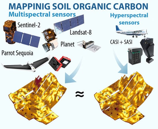
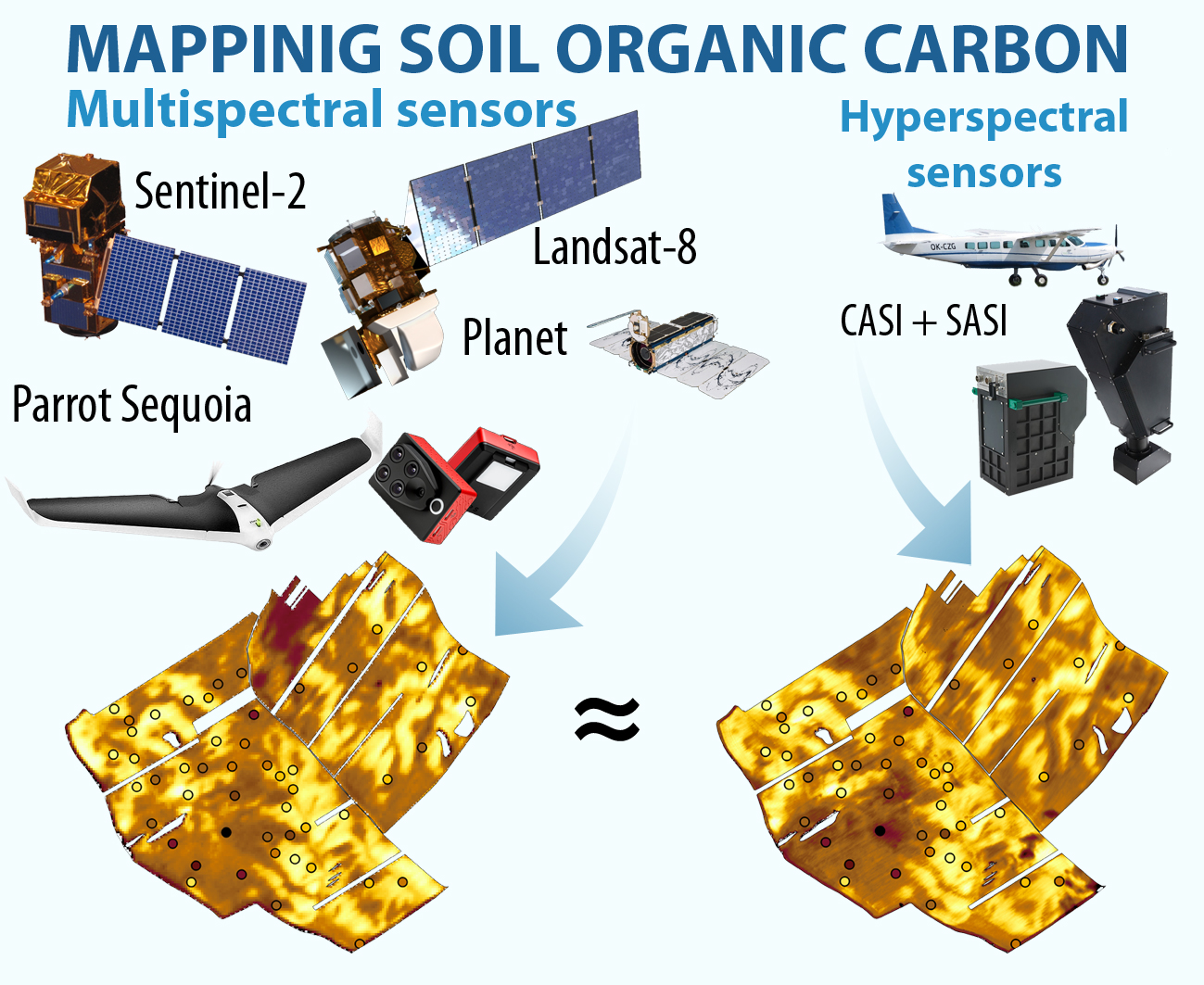
Soil Organic Carbon Mapping Using Multispectral Remote Sensing Data: Prediction Ability of Data with Different Spatial and Spectral Resolutions

Abstract

The image spectral data, particularly hyperspectral data, has been proven as an efficient data source for mapping of the spatial variability of soil organic carbon (SOC). Multispectral satellite data are readily available and cost-effective sources of spectral data compared to costly and technically demanding processing of hyperspectral data. Moreover, their continuous acquisition allows to develop a composite from time-series, increasing the spatial coverage of SOC maps. In this study, an evaluation of the prediction ability of models assessing SOC using real multispectral remote sensing data from different platforms was performed. The study was conducted on a study plot (1.45 km²) in the Chernozem region of South Moravia (Czechia). The adopted methods included field sampling and predictive modeling using satellite multispectral Sentinel-2, Landsat-8, and PlanetScope data, and multispectral UAS Parrot Sequoia data. Furthermore, the performance of a soil reflectance composite image from Sentinel-2 data was analyzed. Aerial hyperspectral CASI 1500 and SASI 600 data was used as a reference. Random forest, support vector machine, and the cubist regression technique were applied in the predictive modeling. The prediction accuracy of models using multispectral data, including Sentinel-2 composite, was lower (RPD range from 1.16 to 1.65; RPIQ range from 1.53 to 2.17) compared to the reference model using hyperspectral data (RPD = 2.26; RPIQ = 3.34). The obtained results show very similar prediction accuracy for all spaceborne sensors (Sentinel-2, Landsat-8, and PlanetScope). However, the spatial correlation between the reference mapping results obtained from the hyperspectral data and other maps using multispectral data was moderately strong. UAS sensors and freely available satellite multispectral data can represent an alternative cost-effective data source for remote SOC mapping on the local scale.

1. Introduction

The decreasing soil organic carbon (SOC) content in agriculture soils is generally considered a major threat to the sustainability of soil cultivation. Its role is essential in many production and non-production soil functions as it controls the dynamics of various agrochemical processes in the soil. The natural equilibrium of the soil environment is endangered due to external, primarily anthropogenic effects, which lead to the development of several degradation processes. These can also affect the soil carbon stocks, especially in the topsoil layer. Soil is a vast carbon pool (the largest terrestrial) [1,2,3,4], making it an essential component of the entire carbon cycle on Earth, especially in the context of expected climate and land-use changes [5,6,7,8]. Therefore, recent research on SOC has received considerable attention. Monitoring, mapping, and describing the spatial variability of SOC (in landscape and also within-field scale) are the key prerequisites for understanding the effects of agricultural practices on SOC changes. Digital soil mapping methods are used to obtain this mapped variability using field sampling and additional environmental covariates [9]. Remote sensing (RS) data represents one of the available data sources for such purposes within large areas. The data are also provided in a sufficient spatial resolution suitable even for local monitoring and applications [10].

A number of studies [11,12,13,14,15,16,17,18,19,20,21,22] have proven that aerial image hyperspectral data with many narrow spectral bands in VNIR-SWIR offer efficient input data to map the spatial variability of important soil properties. Compared to the costly and technically demanding processing of aerial hyperspectral data, multispectral and superspectral satellite data [23,24,25,26,27,28], or multispectral and hyperspectral UAS data [29,30,31] could be a readily available source of spectral data for regular application. Despite the increasing number of respective studies, the potential of this type of data has not been fully exploited. An important point to be addressed is the effect of different spectral and spatial resolutions on prediction ability. It is assumed that reduced spectral resolution, as in the case of multispectral data, results in a reduction in the model’s predictive capability. Despite this, a number of studies dealing with multispectral data [32,33,34] have shown that results can be satisfactorily applied to the needs of precision farming, especially with regard to acquisition costs.

Nevertheless, potential inaccuracies in the outputs resulting from the use of remote RS data with lower spectral resolution and, in the case of satellite sensors, often with coarser spatial resolution, need to be considered. For example, sensors on Sentinel-2 and Landsat-8 satellites covering important organic matter absorption bands in both the visible and SWIR regions of the spectrum may have considerable potential for detailed mapping of SOC. However, only a few studies have confirmed this potential [35,36,37]. Sensors with very high spatial resolution but only covering the VNIR spectrum (e.g., WorldView, Cartosat, Pléiades, and Deimos) are considered less applicable. However, as shown by Crucil et al. [30] in a study comparing UAS-compatible multispectral and hyperspectral sensors operating only in the VNIR spectrum, similar results can be achieved with these sensors compared to reference hyperspectral data also using the SWIR spectrum. Unlike spectral resolution, spatial resolution is considered to have less of an effect on predictions relative to continuously changing soil properties. For example, Castaldi et al. [36] showed that the spatial resolution of Sentinel-2 is adequate for SOC variability mapping both within the field and at a regional scale.

The signal-to-noise ratio (SNR) of sensors is another important issue that affects the prediction ability. Large noise interference in the acquired data associated with the short acquisition time at the investigated location is a disadvantage mainly for satellite data [38,39,40], especially when data are scanned in narrow spectral bands and with high spatial resolution. For example, SOC prediction using the Hyperion hyperspectral satellite sensor [41,42,43,44,45,46,47] may be affected by this phenomenon. A comparison of data from Hyperion and Advanced Land Imager (ALI) sensors [37] showed that sensors with lower spectral resolution but higher SNR can provide better results for SOC prediction.

It follows from the above mentioned that there are still a number of uncertainties and unanswered questions about using the mentioned approaches in management practices. One reason is the difficulty of comparability and hence the possibility of evaluating results from individual studies using different sensors, preprocessing of spectral data, or statistical and numerical data processing techniques. Moreover, accuracy and prediction ability are often affected by other factors, such as different soil conditions, variability of the analyzed characteristics, the condition of the studied surface (moisture and surface roughness affecting vegetation and crop residues), various atmospheric conditions and light incidence geometry during image acquisition [48,49]. This leads to reduced predictive ability compared to that obtained with soil laboratory spectroscopy [33,50] and makes it difficult to map SOC at a large scale, especially in temperate regions, due to crop cover and various types of land parcel management.

There is only a portion of bare soil with a dry and non-rough surface in each RS image. Time series of individual images [51,52,53,54] or multitemporal composites of spectral data can be used to reduce the influence of different surface conditions and eliminate vegetation. Exposed Soil Composite Mapping Processor (SCMaP) [55], Geospatial Soil Sensing System (GEOS3) [56], Bare Soil Composite Image [57], and Barest Pixel Composite for Agricultural Areas [58], all developed from Landsat time series, multitemporal bare soil image [59] developed from RapidEye time series, or bare soil mosaic [60] derived from Sentinel-2 data can serve as examples of such composites. However, only some of the composite products have been used to predict SOC [57,58,59]. Promising results were achieved; however, the potential of these spectral composites has not yet been tested in a relevant number of studies, and further research is needed for its evaluation.

The objective of this study is to critically evaluate the capability of easily accessible data (and one commercially available source with very high spatial resolution) from different types of multispectral sensors to predict within-field variability of topsoil SOC concentration at a local scale. Real spectral image data, identical sampling and processing design, and similar surface conditions (dry conditions and minimal surface roughness) were ensured to achieve this goal. The data from currently operating sensors, including satellite data from Sentinel-2 and Landsat-8 with VNIR and SWIR bands, very-high-resolution data from CubeSat miniature Dove satellites from PlanetScope (VNIR), and data from the UAS-mounted Parrot Sequoia sensor (VNIR) were compared. Multitemporal bare soil composite of Sentinel-2 spectral data was also tested to evaluate the usability of this regional product for regular usage in local mapping. Mapping results from airborne hyperspectral data also used in preliminary studies [14,61] were used as reference data for evaluating the spatial concordance among resulting maps and to analyze the importance of different spectral bands for SOC mapping. Although more datasets with wider variety of spectral and spatial parameters would be needed for a robust analysis and statistical testing, the study attempts to compare the SOC prediction models using real-world data from different sensors to evaluate the influence of spectral and spatial resolution and SNR on prediction accuracy. The hypothesis is that lower spectral and spatial resolution and SNR of image spectral data will lead to lower prediction accuracy.

2. Materials and Methods

2.1. Study Site

The study site is in Šardice, with an area of 1.45 km² (48° 56′ N, 17° 1′ E), located in South Moravia, Czech Republic (Figure 1). It is an agricultural area consisting of three plots with relatively steep slopes and no conservation tillage practices. The mean slope of the study site is 4.2°, with a maximum of around 20°. The region is characterized by mean annual precipitation of 549 mm and mean annual temperature of 9.3 °C. Bedrock was formed by upper Eocene molasse facies (sandstones, conglomerates, and marls) covered by Pleistocene loess forming soil parent material. The thickness of the loess layer varies from several meters to several tens of meters. Calcic Chernozems on loess are the main original soil type in the study site. However, due to steep slopes and agricultural management practices, soil cover has been transformed by intensive erosion (especially water and tillage) and deposition processes. Haplic Calcisols have developed on the steep slopes, and deep colluvial soils have formed in concave parts of the slopes [62,63,64].

2.2. Materials

Data from several multispectral sensors were used to assess the influence of spatial and spectral resolution on prediction accuracy. We focused on commonly available data at different scales and compared high-resolution multispectral images from Landsat-8 and Sentinel-2, and very-high-resolution data from PlanetScope satellites and the UAS multispectral sensor Parrot Sequoia. The individual missions’ characteristics are summarized in

Table 1. Main radiometric characteristics of multispectral and referenced hyperspectral sensors used in this study.

Sensor Characteristics	Sentinel-2 MSI [65,66]	Landsat-8 OLI [67]	PlanetScope [68,69]	Parrot Sequoia	CASI 1500 and SASI 600 [70]
Mission	Spaceborne	Spaceborne	Spaceborne	UAS	Airborne
Sensor type	Pushbroom	Pushbroom	Frame with split-frame NIR filter	4 × 1.2 Mpix Global shutter frame sensors	Both pushbroom
Spectral bands	13	9	4	4	CASI: 72 * SASI: 100 *
Used spectral bands	10	8	4	4	102
Spectral range (nm)	9 VNIR 3 SWIR	5 VNIR 3 SWIR 1 PAN	4 VNIR	4VNIR	CASI: 365–1050 SASI: 950–2450
FWHM (nm)	20–200	18–238	40–90	10–40	CASI: 10 * SASI: 15 *
SNR (typical)	129@444 nm 154@497 nm 168@560 nm 142@664 nm 117@704 nm 89@740 nm 105@783 nm 174@843 nm 72@865 nm 114@943 nm 50@1377 nm 100@1613 nm 100@2200 nm	130@443 nm 130@482 nm 100@561 nm 90@655 nm 90@865 nm 100@1609 nm 100@2201 nm 80@590 nm 50@1373 nm	151@475 184@545 157@655 157@835	Dark target: 27@550 nm * 28@660 nm * 35@735 nm * 30@790 nm * Light target: 39@550 nm * 43@660 nm * 46@735 nm * 41@790 nm *	CASI: 800–900 Peak avelength SASI: 350–450@1000–1350 nm 250–350@1450–1800 nm 100@1900–2350 nm Peak wavelength
GSD (spatial resolution)	10/20/60m	30 m (15 m PAN)	3.5–4m	Variable (cm)	CASI: 1.2 m* SASI: 3.1 m*
Positional accuracy	12 m	12 m	10 m	2 m	1.8 m*
Acquisition date	18-08-2018	19-08-2018	29-08-2018	20-08-2018	21-09-2015

MSI: Multispectral instrument; OLI: Operational land imager; UAS: Unmanned aircraft system; NIR: Near-infrared; FWHM: Full width at half maximum; SNR: Signal-to-noise ratio (@: at specified wavelength); GSD: Ground sampling distance; PAN: Panchromatic. * Values for data used in this study.

, which also presents acquisition times for the datasets. Acquisition times of satellite sensors were chosen to meet two criteria: Firstly, bare soil without crop residues occurred in the images and the soil surface was in a condition minimizing the effects of wetness and surface roughness (dry condition, ploughed, and harrowed). Secondly, the images should be acquired at approximately the same time.

2.2.1. Landsat-8

Landsat-8 was launched in 2013. There are two sensors on board: Operational Land Imager (OLI) collects the data for nine shortwave bands, and Thermal Infrared Sensor (TIRS) for two longwave thermal bands. We used the Landsat-8 OLI surface reflectance data (Level 2 scientific products). Landsat-8 OLI surface reflectance data are generated using the Landsat Surface Reflectance Code, which uses climate data from MODIS as input to a radiative transfer model [71]. The data were requested and downloaded from the EarthExplorer data portal.

2.2.2. Sentinel-2

One individual cloud-free Sentinel-2B image resampled to 10 (downscaling of 20 m bands to 10 m resolution while maintaining original values), 20 and 30 m and soil reflectance composite were used for the analysis. An individual image with the acquisition date 19 August 2018 was downloaded from the ESA Sentinels Scientific Data Hub. We used the Level 2A data product processed by the Sen2Cor processor, which is ready to analyze because geometric, radiometric, and atmospheric corrections are made in preprocessing by the data producer. The whole protocol is described in the Sentinel-2 user handbook [65].

2.2.3. Sentinel-2 Bare Soil Composite

A soil reflectance composite image was processed based on the methodology of exposed Soil Composite Mapping Processor (SCMaP) [55]. Instead of using Landsat data originally used to create SCMaP, Sentinel-2 Level 2A images from March 2017 to May 2019 were used to make the composite. The eo-learn Earth observation processing framework in Python using Copernicus Sentinel data acquired through Sentinel Hub (Sinergise Ltd.) was applied for time series processing. A cloud mask was created by combining data from a scene classification (SCL) map as a product of the Sen2Cor algorithm and data obtained by cloud classification using the Sentinel Hub Cloud Detector for Sentinel-2 images in Python (s2cloudless [72]). The threshold for bare soils was identified based on the PV index, a modification of the normalized difference vegetation index (NDVI) (for details, see [55]). The threshold of the PV index was set to 0.8 based on the investigation of images from data with known soil cover. The resulting soil reflectance composite value was calculated as mean reflectance in individual bands of cloud-free pixels matching the criteria of PV threshold.

2.2.4. PlanetScope

Each PlanetScope Dove satellite is a CubeSat 3U operating in low orbit (400, 475 km) collecting high-resolution optical data in the visible and near-infrared spectra [73]. We used one PlanetScope Ortho Scene product at Level 3B (Planet Labs, Inc. San Francisco, CA, USA). Product Level 3B data are ready to use. The data are geometrically corrected by sensor telemetry and modeled, orthorectified, projected, and scaled to surface reflectance in preprocessing by the producer [68]. Atmospheric corrections are processed using 6SV2.1 radiative transfer code, and AOD, water vapor, and ozone inputs are retrieved from MODIS near-real-time data. Data in original spatial resolution and data resampled to 10 and 30 m were used for the analysis.

2.2.5. Hyperspectral Airborne Imaging

Hyperspectral data from the VIS-NIR (370–1040 nm) CASI 1500 sensor and SWIR (960–2440 nm) SASI 600 sensor (Itres Ltd., Calgary, Canada), according to the high spectral and spatial resolution, were used as a reference dataset for a comparison of the capability of other sensors. The data were acquired in September 2015. CASI collected 72 spectral bands with full width at half maximum (FWHM) of 15 nm and spatial resolution of 1.2 m. SASI collected 100 spectral bands with FWHM of 10 nm and spatial resolution of 3.1 m. The Global Change Research Institute of the Czech Academy of Sciences located in Brno conducted the acquisition and preprocessing. The preprocessing phase involved radiometric, geometric, and atmospheric corrections (ATCOR-4). A detailed description of the image acquisition and preprocessing is given in [14]. Results from previous studies [14,61] using spectra transformed by Savitzky–Golay filter (third-order polynomial smoothing and 5-band window widths) with first derivative were used as reference data. Raw reflectance data at original resolution were used for comparative analysis, as well as raw data resampled to 10 and 30 m spatial resolution.

2.2.6. UAS Multispectral Imaging

A Parrot Disco Pro AG set combining the Parrot Disco Pro fixed-wing with multispectral Parrot Sequoia camera (Table 1) mounted on the board was used in the study. Parrot Sequoia captures images in the four independent spectral bands and with a red-green-blue (RGB) sensor. Each channel is acquired by an independent camera with a fixed lens, 1.2 megapixels (1280 × 960 pixels) global shutter monochrome sensor capturing data in four narrow bands: Green (550 nm, FWHM 40 nm), red (660 nm, FWHM 40 nm), red edge (735 nm, FWHM 10 nm), and near-infrared (790 nm, FWHM 40 nm). Unfortunately, the RGB sensor of the camera has a slow rolling shutter sensor, resulting in very difficult or even impossible RGB data processing. The position from on board the global navigation satellite system (GNSS) and inertial navigation unit is stored in exchangeable image file format (EXIF) metadata files. The camera is also connected to a sunshine sensor and the irradiance data are stored in the EXIF files.

Multispectral image acquisition was conducted by the authors on 20 September 2018 at around 12:00. The sky was clear. The flight plan was prepared by the Pix4Dcapture mobile app for iOS. The flight proceeded automatically at an altitude of 70 m covering an area of 35 ha in a single flight (100 ha in three flights), resulting in 1600 multispectral images with a spatial resolution of 6.5 cm. Unfortunately, the whole area was not covered by UAS imaging, because we did not have enough batteries for the UAS to fly over the whole study area; only three accumulators from the set were available. Images were captured at specified automatically calculated positions consistent with 80% frontal and 70% side overlap. Reference ground calibration images of five calibration targets with known reflectance measured in the laboratory were captured directly before the flight. The main purpose was to compensate for ambient atmospheric conditions and the influence of sun angle.

The SNR of the Parrot Sequoia camera was calculated from the lightest and darkest calibration targets according to Ben-Dor and Levin [74]. The DN values of the targets were extracted from the calibration images for all bands. The SNR estimation was then calculated according to Equation (1):

SNR = AV/SD

(1)

where AV is the average DN value of pixels (signals) over a homogeneous target and SD represents noise estimated from the standard deviation of DNs.

Photogrammetric processing was performed using AgiSoft Metashape Professional 1.5.0 (AgiSoft LLC, St. Petersburg, Russia). Metashape allows 3D reconstruction of the scene to be performed from the imagery, employing the structure from motion and semi-global matching algorithms. The reliable performance of the software in photogrammetric processing has been proven in previous studies (e.g., [75]). Moreover, Metashape contains the Sequoia camera model and it can automatically extract the information about cameras and sun sensors directly from EXIF files.

All 1600 multispectral images acquired in the imaging campaign over the study area were included in the orientation processing. The near-infrared band was set as a master channel for computing image orientations in the WGS 84 coordinate system. Only GNSS onboard data were used for photo alignment. Then, radiometric calibration was conducted using an empirical line method implemented in the software. The five calibration targets were masked on the picture (one for each target) in all bands. The masks were paired with appropriate reflectance values. The radiometric calibration was then computed automatically. The following steps in the workflow consisted of dense cloud generation and automatic ground point classification. Based on these datasets, the digital terrain model (DTM) and orthomosaic with surface reflectance values were generated. Reflectance data resampled to 1 and 10 m spatial resolution were used for the purpose of SOC prediction.

2.3. Methods

2.3.1. Collection of Soil Sampling Data

Study plot investigation and soil sampling were carried out during the field campaign following the aerial hyperspectral flight campaign on 6 April 2016. Soil conditions of the plot were investigated with 1 m deep auger boreholes. An optimized network of borings fashioned using a conditioned Latin hypercube sampling (cLHS) [76] stratified random strategy was used for observation and soil sampling. Image-based spectral data and terrain attributes derived from the digital elevation model (5 × 5 m² resolution digital terrain model of Czech Republic of the fourth-generation DMR 4G^® with total standard error of 0.3 m for height in bare terrain) were used as feature space variables. A total of 50 borings were recorded (descriptions of soil unit, soil depth, and soil profile stratigraphy) and 50 composite samples (3–5 samples covering area of 1 m²) were taken from these sites at 0–10 cm depth. Geographic positions of borings were measured by a Trimble GeoXM GPS receiver, with a postprocessing accuracy of approximately 1 m. The soil samples were analyzed for SOC and texture class based on a standard laboratory procedure (air-drying, grinding, and sieving with a 2 mm sieve; ISO11464: 2006). SOC was analyzed as total oxidized carbon and measured using wet oxidation (ISO14235: 1998).

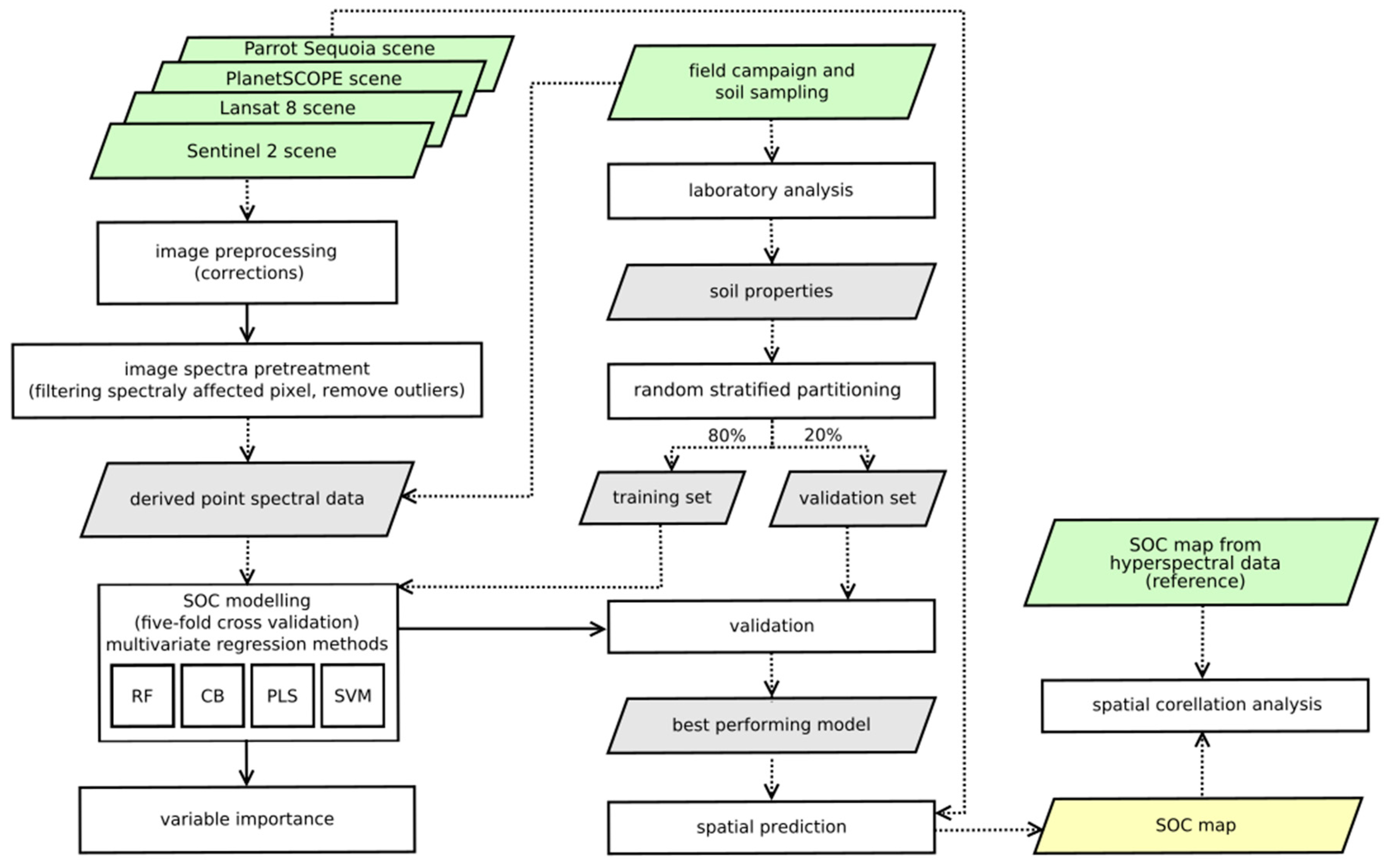
2.3.2. Prediction of SOC

Digital soil mapping methods were used for predictive modeling of SOC using image spectral data in the spatial domain. Different multivariate regression techniques were applied because of the inability to define the best model for specific conditions. Random forest (RF) [77], support vector machine (with linear, polynomic, and radial kernels) (SVM) [78,79,80], cubist (CB) [81], and partial least squares (PLS) [82] were used as techniques previously applied successfully in DSM and soil imaging spectroscopy. Only spectral data characterized by surface reflectance in individual bands were used as covariates (independent variables) in models in order to analyze the influence of different spectral data characteristics on the ability to predict soil properties. The process of fitting the models, calibrating and validating the results, and making final predictions was the same for all input spectral data. Caret packages [83] in R software (R Development Core Team, Vienna, Austria) were employed for all processing steps in the prediction modeling procedure.

The processing steps (see flowchart in Figure 2) were as follows:

• Spectrally affected pixels in individual data sources were filtered based on NDVI value. The threshold was set to 0.25 according to a preliminary analysis of bare soils within the study area. Only 0 to 2 samples from the whole dataset (50 samples) were filtered, depending on the data source.
• The filtered dataset was partitioned into a training set (for calibration purposes) and a test set (for validation purposes) as independent validation data were not available [84]. Partitioning at a 4:1 ratio was carried out by random stratified sampling based on predicting variable (SOC) values (grouped based on 10th percentile) ensuring the same distribution of both datasets and enabling a balanced comparison of results.
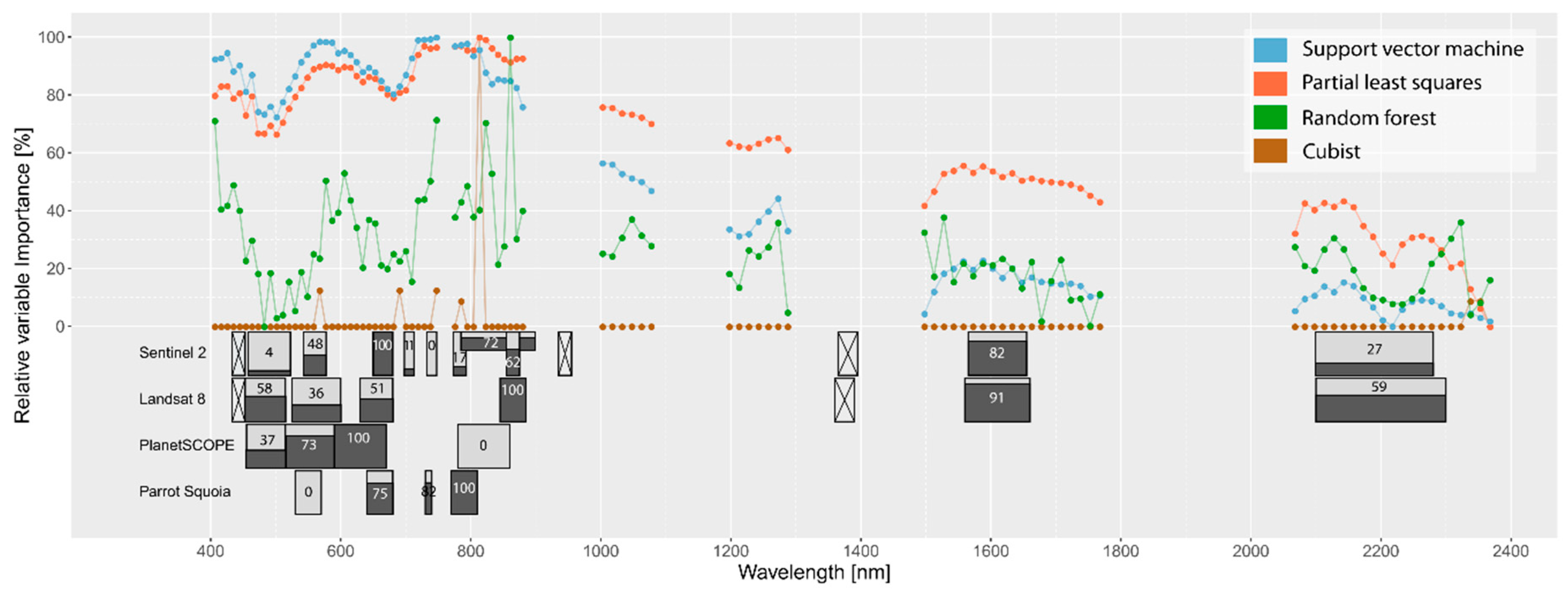
• The training process included fitting separate models. Five-fold cross-validation of the training set was used to assess the model performance and find model parameters. The best parameters were optimized and selected by a grid search. These parameters included a number of latent variables for PLS and hyperparameters for machine learning methods (RF—number of randomly selected predictors and number of trees to grow, CB—number of committees and number of instances, SVM—cost for linear kernel; cost and sigma for radial kernel; polynomial degree scale and cost for polynomial kernel). Model specific metrics was used in each model for the calculation of the importance of variables (spectral bands) (CB—usage as a linear combination of the rule conditions and terminal model; RF—increase in mean squared error by permuting a variable; PLS—weighted sums of the absolute regression coefficients) with the exception of SVM, where the squared weights [85] were used. Importance values were standardized to range 0–100. The final model was selected based on the smallest root mean square error of cross-validation (RMSECV) value. This model was used in the next step for validation of the validation set.
• The prediction ability of models and accuracy of prediction were evaluated by determining the measure of accuracy computed based on a comparison of observed and predicted values of the validation set. Root mean square error of prediction (RMSEP), coefficient of determination (R²), and Lin’s concordance correlation coefficient (CCC) were computed. Even though some measures may have duplicate meanings [86], they are often used together by many authors, and we also calculated the ratio of performance to deviation (RPD) and the ratio of performance to interquartile range (RPIQ), which are more suitable for datasets with skewed distribution [87].
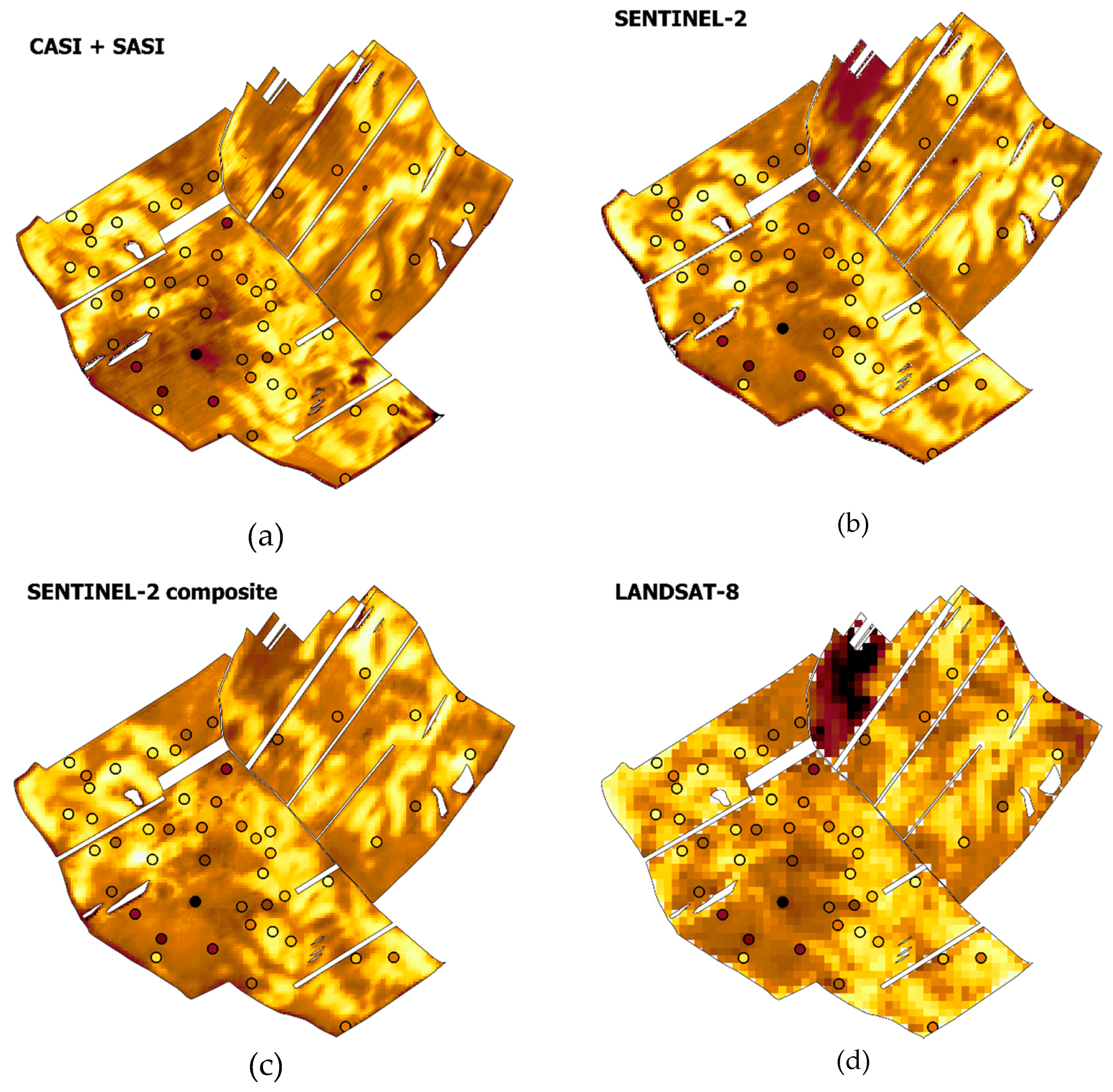
• Finally, the spatial prediction of soil attributes was performed using a selected model with the best predictive ability (lowest RMSEP value). This model was applied to the entire dataset of image spectral data.

3. results

3.1. Descriptive Statistics of Soil Samples

Descriptive statistics of SOC content in the study site, including mean, minimum, maximum, range, standard deviation (SD), coefficient of variation (CV), and interquartile range (IQ), are shown in

Table 2. Descriptive statistics of content (%) of main soil properties. SD: Standard deviation; CV: Coefficient of variation; IQ: Interquartile range.

Soil Properties	Min	Max	Mean	Range	SD	CV (%)	IQ
SOC (%)	0.84	2.62	1.44	1.78	0.39	27	0.51
Sand (%)	15.2	58.3	38.91	43.1	8.34	21.4	10.0
Silt (%)	27.5	49.1	38.49	21.6	4.67	12.1	4.45
Clay (%)	14.2	48.3	22.6	34.1	6.8	30.1	5.93
CaCO3 (%)	0	10.0	4.07	10.0	3.34	82.1	6.56

. There is a high SOC within-field spatial variability in the topsoil in the site due to the long-term effect of erosion processes compared to sites in the same area with flat topography. The SOC content ranges from 0.84% to 2.62% (mean 1.44%) and is classified as low to high. The highest values have been found in places with autochthonous Calcic Chernozems only weakly affected by erosion (range 1.24%–2.62%, mean 1.86%). On the other hand, significantly lower content has been found in eroded soils (Haplic Calcisols) on the most exposed terrain positions in terms of tillage and water erosion (range 0.84%–1.84%, mean 1.27%). Compared to the assumptions, there was low to moderate carbon content in the topsoil of the colluvial soils (range 1.04%–1.57%, mean 1.33%).

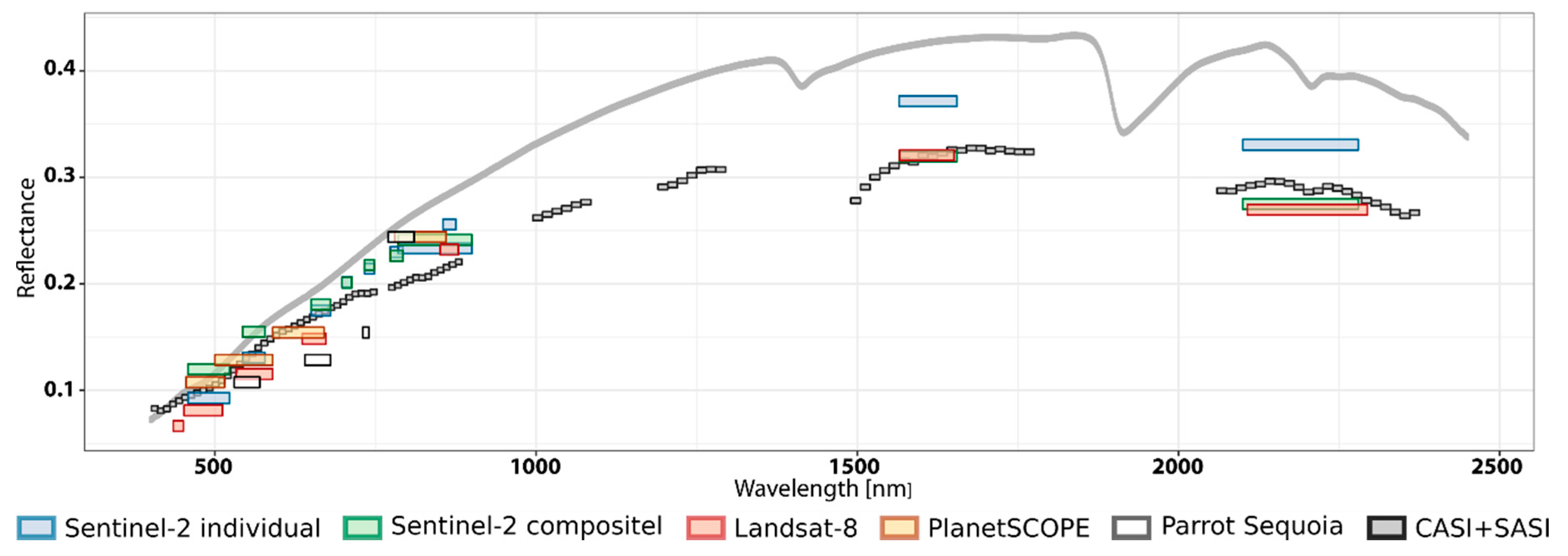
3.2. Comparison of Measured Spectra

Even though spectral data were collected at similar times under the same surface conditions (in dry periods with no change of roughness), reflectance data showed significant differences. The reflectance values measured by the sensors used are depicted in Figure 3 as mean reflectance from all samples. The lowest differences were found predominantly in NIR bands of all multispectral sensors, where the range of values is about 0.025. More pronounced differences were observed in the visible parts of spectra, where the lowest value of reflectance is related to UAS-based reflectance measurements with Parrot Sequoia, followed by Landsat-8 and PlanetScope. The differences in these parts of the spectra reach 0.05 of reflectance. The PlanetScope data show the highest match with aerial hyperspectral data in visible spectra. The closest match in the SWIR region, where only Sentinel-2 and Landsat-8 have spectral bands, was found for data from Landsat-8 and Sentinel-2 composite, while individual Sentinel-2 data exceed reflectance by about 0.05.

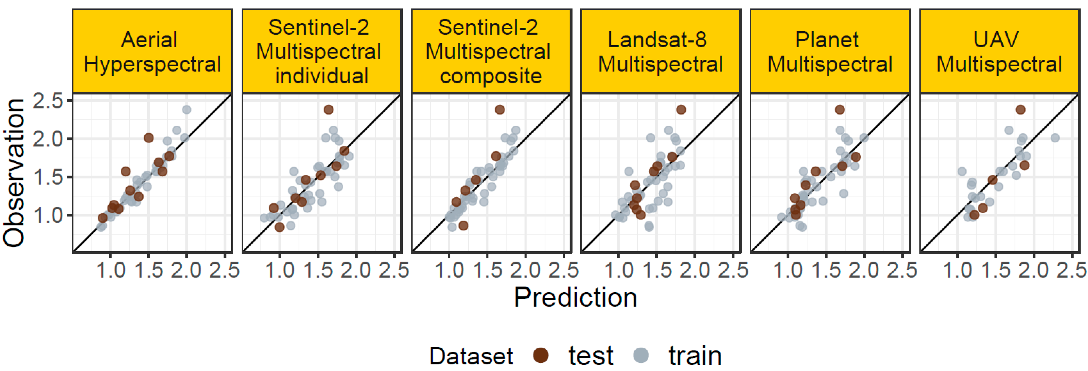
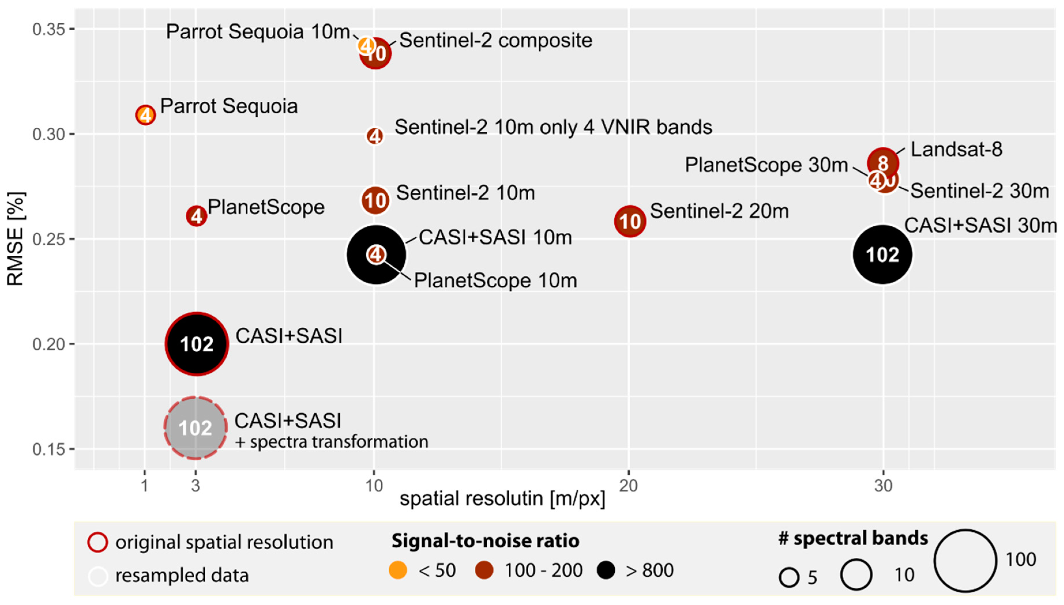
3.3. Prediction of Soil Properties by Spectral Data

The statistical accuracy obtained using the multispectral data was lower compared to the hyperspectral data (see results in Figure 4 and Figure 5 and

Table 3. Prediction accuracy obtained by modeling with different sensors.

Platform	SR (m)	No. of Bands	Total Samples	Best Model	Calibration			Validation
					No. of Samples	RMSECV (%)	R2cv	No. of Samples	RMSEP (%)	R2p	CCC	RPD	RPIQ
Sentinel-2 individual	10	10	50	PLS	40	0.29	0.72	10	0.27	0.66	0.75	1.45	1.88
Sentinel-2 individual	20	10	50	CB	40	0.24	0.7	10	0.26	0.68	0.69	1.52	2.00
Sentinel-2 individual	30*	10	50	CB	40	0.25	0.64	10	0.28	0.56	0.64	1.4	1.80
Sentinel-2 composite	10	10	49	CB	39	0.28	0.52	10	0.34	0.81	0.62	1.16	1.53
Landsat-8	30	8	49	SVM	39	0.29	0.45	10	0.28	0.65	0.65	1.41	1.86
PlanetScope	3	4	49	CB	39	0.20	0.75	10	0.26	0.66	0.74	1.52	2.00
PlanetScope	10	4	49	RF	39	0.22	0.64	10	0.24	0.74	0.80	1.65	2.17
PlanetScope	30	4	49	RF	39	0.21	0.70	10	0.27	0.59	0.72	1.46	1.93
Parrot Sequoia	1	4	29	CB	23	0.27	0.72	6	0.31	0.72	0.7	1.38	1.77
Parrot Sequoia	10	4	29	CB	23	0.28	0.52	6	0.34	0.57	0.68	1.26	1.62
CASI + SASI	3	102	48	SVM	39	0.16	0.82	9	0.20	0.76	0.86	1.81	2.68
CASI + SASI * + SG trans.	3	102	48	SVM	39	0.17	0.87	9	0.16	0.8	–	2.26	3.34
CASI + SASI	10	102	48	SVM	39	0.17	0.80	9	0.24	0.73	0.76	1.51	2.23
CASI + SASI	30	102	48	SVM	39	0.16	0.82	9	0.24	0.63	0.73	1.51	2.23

* Reference data [14]. Bold font indicates data in original spatial resolution, others are resampled from original resolution. SR: Spatial resolution; RMSE_CV: Root mean square error of cross-validation; RMSE_P: Root mean square error of prediction; CCC: Lin’s concordance correlation coefficient; RPD: Ratio of performance to deviation; RPIQ: Ratio of performance to interquartile range; PLS: Partial least squares; CB: Cubist; SVM: Support vector machine; RF: Random forest; SG: Savitzky–Golay spectral transformation.

). The most accurate prediction of SOC content, achieved with reference aerial hyperspectral data preprocessed by spectral transformation (RMSE = 0.16%; RPD = 2.26; RPIQ = 3.34; R² = 0.8), can be considered an achievable limitation of prediction accuracy. The hyperspectral data had the highest spectral resolution (112 bands) and SNR in combination with high spatial resolution (3 m). Prediction using only raw hyperspectral data without any spectral transformation showed lower performance (RMSE = 0.20%; RPD = 1.81; RPIQ = 2.68; R² = 0.76). A greater reduction in prediction performance was found using hyperspectral data resampled to 10 and 30 m resolution (RMSE = 0.24%; RPD = 1.51; RPIQ = 2.23).

The prediction accuracy of the individual Sentinel-2 image with a ground sampling distance of 20 m was slightly higher (RMSE = 0.26%; RPD = 1.52; RPIQ = 2) compared to Landsat-8 with 30 m spatial resolution (RMSE = 0.28%; RPD = 1.42; RPIQ = 1.85). The prediction accuracy of the model using Sentinel-2 data resampled to Landsat-8 30 m resolution was slightly lower (RMSE = 0.28%; RPD = 1.40; RPIQ = 1.81) compared to the original Sentinel-2 data. However, results show great agreement with the results using Landsat-8 itself.

Despite having the finest spatial resolution, the lowest accuracy was achieved by using UAS mutispectral data (RMSE = 0.31%; RPD = 1.37; RPIQ = 1.77). Only 29 samples could be used for UAS modeling, due to limited coverage of image data. These data, and PlanetScope data, cover only VNIR spectral regions. Nevertheless, the prediction accuracy of the model using PlanetScope data with very high resolution (3 m) was comparable (RMSE = 0.26%; RPD = 1.52; RPIQ = 2.00) to the original Sentinel-2 individual image and slightly higher than Landsat-8. The prediction slightly improved when using PlanetScope data resampled to 10 m (RMSE = 0.24%; RPD = 1.46; RPIQ = 1.93). Resampling to 30 m led to a further decrease in prediction accuracy (RMSE = 0.27%; RPD = 1.46; RPIQ = 1.93). The least Sentinel-2 composite data showed the lowest prediction ability (RMSE = 0.34%; RPD = 1.16; RPIQ = 1.53).

Figure 5 shows a between-sensor comparison of RMSE of prediction according to the spatial resolution and the number of spectral bands (numbers within points). There is no substantial trend in RMSE values regardless of spatial and spectral resolution for all multispectral platforms.

The importance of spectral bands in models with native spatial resolution was investigated in greater depth to determine the bands most appropriate for SOC modeling and the difference between the sensors. Standardized variable importance coefficients are depicted in Figure 6. The importance characteristics for hyperspectral data show similar trends in each of the used regression models. The bands in the visible and NIR spectrum are of the utmost importance, with maxima in NIR. The importance decreases continuously up to the SWIR spectrum. The red and NIR bands are the most significant in the multispectral data. The only exception PlanetSCOPE data, where the NIR band did not show a significant importance in the prediction model. SWIR bands for Sentinel-2 and Landsat-8 were also very important prediction bands, especially SWIR 1 band around 1600 nm.

Figure 7 depicts the predicted SOC spatial distribution compared with the observed values. The maps are derived from predictive modeling based on different sensor data. All maps show similar coherent patterns of SOC variability regardless of spatial resolution. The spatial correlation analysis (Pearson correlation coefficient) was used to assess the concordance among the resulting maps. The results are shown in the correlation matrix in

Table 4. Correlation matrix with overall correlation metrics between maps.

	CASI + +SASI	Sentinel-2	Sentinel-2 Composite	Landsat-8	PlanetScope
Sentinel-2	0.756
Sentinel-2 Composite	0.761	0.883
Landsat-8	0.622	0.732	0.715
PlanetScope	0.817	0.797	0.773	0.648
Sequoia	0.748 1	0.833 1	0.803 1	0.823 1	0.874 1

¹ Values calculated using limited area recorded from Unmanned Aerial Vehicle.

. The best match between the reference map from the hyperspectral data and the multispectral data was obtained for PlanetScope (0.82). The worst result was achieved with Landsat-8 with the lowest spatial resolution (0.622); however, this relationship is also moderately strong.

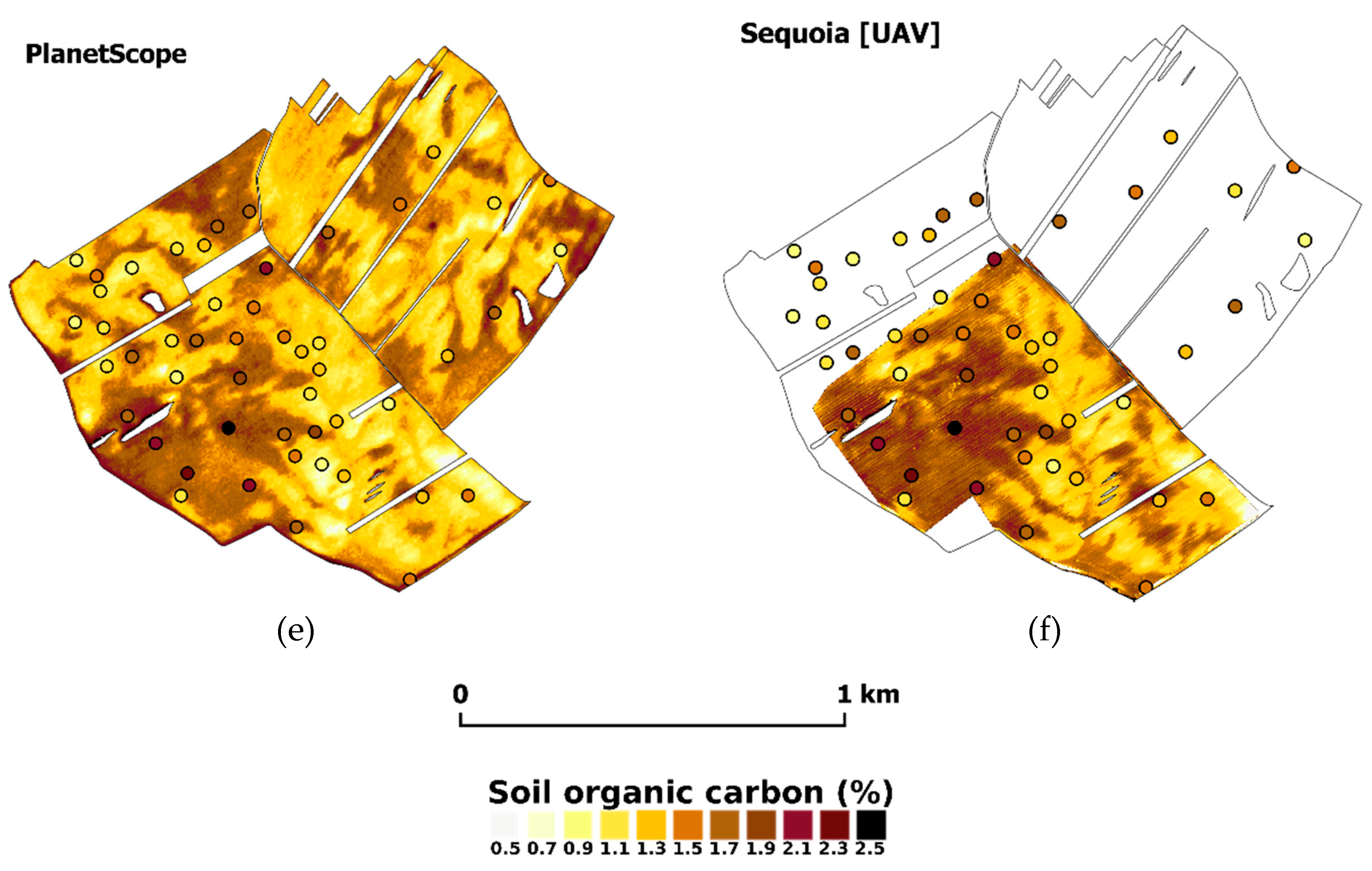
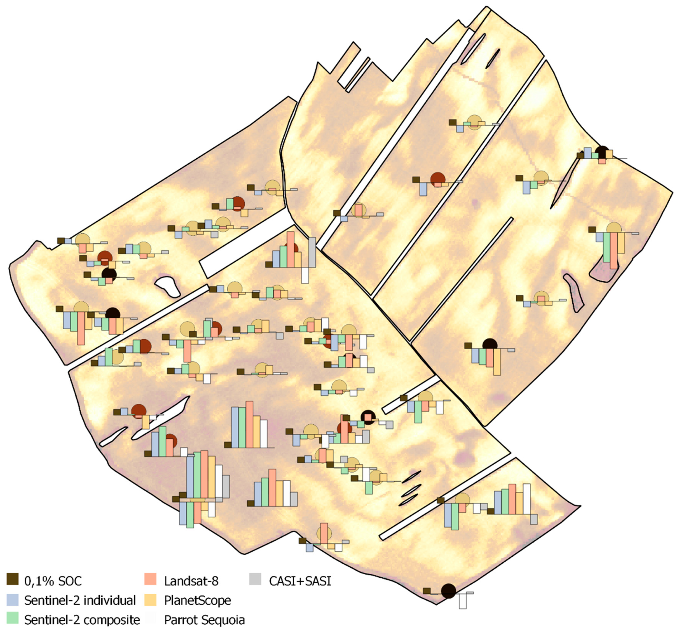
3.4. Spatial Distribution of SOC

Figure 8 shows prediction error values for individual points. The highest prediction errors reach 0.6% SOC. Most errors are related to underestimating actual SOC values, mainly in the original Chernozems with high SOC concentration (SW part of the plot). Another area with an increased prediction error was detected in terrain depressions covered by Colluvial soils. The pattern of prediction errors is similar for all platforms.

4. Discussion

The results showed a potential of different types of multispectral data for mapping SOC on a local scale and even for regional mapping using composite datasets. On the one hand, the predictive capability of models achieved poor or average results based on RPD evaluation (RPD from 1.16 to 1.65). This means that the error of these models is similar or only slightly lower than the standard deviation of the SOC samples. On the other hand, despite these rather inconclusive results, other findings (especially spatial correlation analysis) indicate a high correlation between the reference results obtained from the hyperspectral data and other maps, especially those derived from Sentinel-2 and PlanetScope (0.75 and 0.82). This was shown in the comparison of map outcomes. Thus, the final maps produced on the basis of multispectral data can, despite the low model accuracy metrics, precisely reflect the within-field variability of SOCs. The results (RPIQ values, scatterplots of predictions and observations, and maps) also show that the models predicted worse the values in the lower and upper tails of the distribution. This affects the model accuracy metrics. In this respect, it would be appropriate to address the issue of outliers in future research. It could help to increase the accuracy of the prediction in tailed values, which is generally a problem with machine learning methods. The prediction accuracy of models can also be improved by incorporating other environmental covariates (terrain, parent material maps, etc.) or incorporating covariate contextual information into the prediction models [88,89,90,91,92,93].

The achieved results illustrate that multispectral data provide significantly worse SOC estimations than reference hyperspectral data regardless of the spatial resolution. This is due to the combination of higher SNR and spectral resolution. However, the availability of the hyperspectral data is, due to a lack of hyperspectral satellites in orbit, generally worse. Other drawbacks of the hyperspectral data are a high acquisition cost of aerial data, high demands on hardware, and know-how in the data processing. On the other side, the presented multispectral RS missions, especially Sentinel-2 and Landsat-8, provide large amounts of freely available data that can be suitable for SOC digital mapping. The results of our study show very similar prediction accuracy for all spaceborne sensors with only minor prediction variance, which could not be explained without a full factorial experiment design and consequent statistical testing of all variables. More data from different sensors would be needed for a robust analysis. Despite the limited number of sensors, interesting conclusions have been drawn.

Satellite multispectral sensors provided data only from a few broad spectral bands. This is the difference from the hyperspectral sensors which provide continuous reflectance curves in VNIR-SWIR spectra with high SNR and include more absorption features related to SOC [94,95]. This allows for better results and higher accuracy of SOC prediction. Similar results were reported by Castaldi et al. [42], who compared SOC estimation by the PLSR model using image data from the Advanced Land Imager (ALI) and Hyperion sensors on board the EO-1 satellite. Hyperion data provided better results than multispectral ALI data for clay, sand, and especially for SOC estimation. Cascaldi et al. [37] estimated SOC and other soil properties using simulated data from soil spectral libraries and data from seven hyperspectral and multispectral sensors. Sentinel-2 MSI data showed prediction accuracy equal to simulated Hyperion data, which had very low SNR in the SWIR spectrum, but the Sentinel-2 data had significantly better results in terms of prediction accuracy (RPD = 1.55; RPIQ = 2.68) than Landsat-8 (RPD = 1.46; RPIQ = 2.51). The best results were achieved with EnMAP (RPD = 1.8; RPIQ = 3.11). According to their results, this was due to more bands in the SWIR region combined with narrower bands, which better reflect the spectral features of organic matter. Rosero-Vlasova et al. [96] obtained similar results also using simulated satellite data. They achieved the best fit with models using simulated EnMAP reflectance (R² = 0.93). The least reliable estimates (R² = 0.4) came from the simulated Landsat model, while the Sentinel-2 model showed better performance (R² = 0.63). In our study, we obtained slightly better results using non-simulated real satellite data from Landsat-8 (R² = 0.65, RMSE = 0.28%) and Sentinel-2 (R² = 0.68, RMSE = 0.26%). Moreover, the prediction accuracy of the Sentinel-2 model was slightly better than that of the Landsat-8 model, which is consistent with the aforementioned studies [37,96].

Spectral absorption regions, which can be used to quantify soil organic carbon (SOC), are located mainly in broader bands in the visible region of the spectrum and in the narrower bands of the SWIR spectrum (between 1600 and 1900 nm and around 2100 and 2300 nm) [36,37,97,98,99,100]. For this reason, the spectral resolution of the sensors significantly influences the quality of SOC predictions [34,37]. It is, therefore, necessary to use data with appropriate spectral resolution taken across the VNIR-SWIR spectrum for accurate SOC estimates [101]. This is also shown by the results of our study, where the importance of bands in individual prediction model was investigated. Red and NIR bands are the most important in the multispectral data use (except of PlanetSCOPE data). This suggests that not only the presence of spectral bands but also their constellation is very important. SWIR bands for Sentinel-2 and Landsat-8 were also very important prediction bands, especially SWIR 1 band around 1600 nm. Presence of these bands can be a significant advantage over the data that uses only bands in the visible and NIR spectrum. New-generation satellite hyperspectral sensors (e.g., EnMAP, PRISMA, HyspIRI, SHALOM) with relatively high SNR and high spatial resolution can make progress in this regard. Recent studies have demonstrated their potential for SOC prediction based on simulated data from point hyperspectral measurements [12,37].

Unlike spectral resolution, the effect of spatial resolution is not so obvious. It can be assumed that higher spatial resolution can lead to slightly higher prediction accuracy, if other parameters of the sensors are identical. This was confirmed by the results of the study when upscaling of data led to a decrease in predictive ability—Sentinel-2 data from 20 m (RMSE = 0.26%) to 30 m (RMSE = 0.28%), PlanetScope data from 3 m (RMSE = 0.26%) to 30 m (RMSE = 0.27%), and Parrot Sequoia data from 1 m (RMSE = 0.31%) to 10 m (RMSE = 0.34%). The same trend was achieved by the model using the raw hyperspectral dataset with original spatial resolution of 3 m (RMSE = 0.20%). The hyperspectral datasets rescaled to 10 and 30 m resolution showed a decrease in the prediction accuracy (RMSE = 0.24%). These minor decreases in prediction accuracy could be caused by decreasing spatial resolution of the image, because the spectral resolution remains constant. However, we could not perform statistical testing of the decreasing prediction accuracy trend due to the lack of multiple instances of each rescaled model and its validation metrics. Steinberg et al. [12] similarly investigated the influence of spatial resolution to SOC prediction by PLSR, comparing simulated spaceborne hyperspectral EnMAP and Airborne hyperspectral system (AHS) images with higher spatial resolution. Their results showed that EnMAP allowed prediction of iron oxide, clay, and SOC with an R² between 0.53 and 0.67 compared to AHS imagery with an R² between 0.64 and 0.74.

A great potential for local applications is linked to UAS spectral sensors, as shown by Crucil et al. [30]. The main advantages of UAS data are low acquisition cost, high spatial resolution, and flying on demand. However, the prediction accuracy of the models using images from the Parrot Sequoia UAS camera (R² = 0.72, RMSE = 0.31%) was lower compared to the spaceborne sensors. It should be noted that these sensors are much cheaper and built with inexpensive electronics parts, resulting in significantly lower SNR, which is not comparable with the SNR of agency-funded satellites [102]. Although we do not have enough data to test this hypothesis, it can be assumed that the lower accuracy of Sequoia data is partially influenced by lower SNR. SNR has a proven effect on prediction accuracy [11,37,103]. Gomez et al. [39] concluded that the lower accuracy of SOC estimations using Hyperion spectra is because of lower SNR (~50:1) and spatial resolution compared to Agrispec field spectrometer data resampled to similar spectral resolution.

In this study, predictive ability was also evaluated using a time composite from Sentinel-2 data. The prediction of soil properties using RS data requires the presence of bare soil in the images. Thus, it is necessary to select images without the masking effect of vegetation. Mapping of larger areas accordingly is rather complicated, especially in temperate regions with different crop rotations throughout the year. The use of time composites is one of the few proven alternatives. The main challenges in composite development are cloud masking (and cloud shadows), definition of bare soils (vegetation masking, including non-photosynthetic vegetation, straw, and litter) on individual images and determination of the resulting reflectance values. Different approaches were used to derive the reflectance values of the final product in the previous studies. Thresholds of spectral indices are usually used for the vegetation masking: Mainly NDVI for green vegetation [56,57,59,60], NBR2 [56,104], or MID-infrared [57] for non-photosynthetic vegetation or combined indexes, such as Bare soil index (BSI) [58] or PV [55]. Statistics from time series of masked data were used to derive final reflectance data—mean [55,58], median [56], or minimum [57,60]. Other methods used to improve and obtain more stable values included, for example, exclusion of 5% quartile [58], application of PCA components [54], field-based standard deviation values [59] or using low-pass filter [60]. In this study, we used Sentinel-2 time series, PV index for masking vegetation and mean statistic for deriving reflectance data and Sentinel-2 composite. The prediction using this composite achieved only average results. However, these results were better than those achieved in a study by Diek et al. [58], which was conducted at the national level using Landsat data, and comparable with results of Blasch et al. [59] and Gallo et al. [57]. The potential of these composite data is great; it can be used as an entry in DSM models. However, further development is necessary. It can be assumed that the weak predictive ability of these data is due to various factors. Above all, this product combines data that has been taken under different moisture conditions and surface roughness. Despite a progress in this area, it is necessary to develop new algorithms, not only for identifying bare soils, but also for removing the influence of moisture, surface roughness, or vegetation residues. Clouding and shading effects on input data is another aspect. Clouds and shadows can be masked using already developed algorithms, but the results are still not faultless. Therefore, further development is needed in this respect.

We must take into account that the results can be affected by the mismatch between the size of the sampling spot (composite sample in the area of 1 m²) and the resolution of the sensor (1–30 m²). However, evaluating this effect would require a very challenging experiment going beyond the scope of this research. Thus, further studies are needed to evaluate this effect. Another issue that could negatively affect the results of multispectral models in this study is the sampling design. As mentioned for example by Castaldi et al. [11], one sampling for each remote sensing acquisition is required for a precise prediction. SOC concentration can have strong dynamics in both space and time, and differences in sampling and acquisition time can negatively affect the results. Although organic fertilizers were not applied and no significant erosion events occurred between the time of sampling and data acquisition, it is necessary to take into account the possible influence on the results. Unfortunately, this cannot be achieved without a time-differentiated and time-consuming and costly sampling. According to our best knowledge, any study assessing the effect of sampling and acquisition time on the SOC prediction has not been conducted yet, but is urgently needed.

5. Conclusions

This study aimed to evaluate the capability of multispectral RS data to predict the variability of SOC concentration in the topsoil in the study plot to assess the influence of spectral and spatial resolution on the prediction accuracy of models. The results of this study show that hyperspectral data provide better SOC estimations than multispectral data. However, hyperspectral data are not always freely available and involve high cost and technical demands. On the other side, multispectral RS missions, especially Sentinel-2, provide large amounts of freely available data. The short revisit time, 10 m spatial resolution, and higher signal-to-noise ratio could be highlighted as major advantages of Sentinel-2 compared to some mature hyperspectral sensors. Short revisit times also enable wide time-series databases of Sentinel-2 images to be built and soil reflectance composite to be constructed as an alternative to using individual images. Other research data sources, such as Landsat-8, as well as data with the limited spectral resolution, such as PlanetScope CubeSat data with high spatial and temporal resolution, have shown their potential. The study also shows that the application of UAS sensors for SOC predictive modeling can be a suitable and cost-effective alternative for remote SOC mapping. The main advantages of UAS data are low acquisition cost, high spatial resolution, and flying on demand while maintaining comparable SOC prediction with spaceborne multispectral sensors. Despite efforts in recent years, further progress in increasing the predictive power of these datasets is needed. In conclusion, UAS sensors for SOC estimation at the plot scale and Sentinel-2 data at the regional scale may represent an alternative to the cost-effective data sources for remote SOC mapping. However, the results of the study are limited by the complexity of remote sensing data acquisition and sampling date, the number of used soil samples, and spatial extent of the study. Therefore, more comprehensive studies, especially on a regional scale, are needed.

References

1. Batjes, N.H. World Soil Carbon Stocks and Global Change; ISRIC: Wageningen, The Netherlands, 1995. [Google Scholar]
2. Houghton, R.A. Changes in the storage of terrestrial carbon since 1850. In Soils and Global Change; Lal, R., Kimble, J.M., Levine, E.R., Stewart, B.A., Eds.; CRC Press: Boca Raton, FL, USA, 1995; pp. 45–65. [Google Scholar]
3. Todd-Brown, K.E.O.; Randerson, J.T.; Post, W.M.; Hoffman, F.M.; Tarnocai, C.; Schuur, E.A.G.; Allison, S.D. Causes of variation in soil carbon simulations from CMIP5 Earth system models and comparison with observations. Biogeosciences 2013, 10, 1717–1736. [Google Scholar] [CrossRef]
4. Hiederer, R.; Köchy, M. Global Soil Organic Carbon Estimates and the Harmonized World Soil Database; EUR 25225; Publications Office of the European Union: Luxembourg, 2011; ISBN 978-92-79-23108-7. [Google Scholar]
5. Banwart, S.A.; Black, H.; Cai, Z.; Gicheru, P.T.; Joosten, H.; Victoria, R.L.; Milne, E.; Noellemeyer, E.; Pascual, U. The Global Challenge for Soil Carbon. In Soil Carbon: Science, Management and Policy for Multiple Benefits; Banwart, S.A., Noellemeyer, E., Milne, E., Eds.; CAB International: Wallingford, UK, 2015; pp. 1–9. ISBN 9781780645322. [Google Scholar]
6. Milne, E.; Banwart, S.A.; Noellemeyer, E.; Abson, D.J.; Ballabio, C.; Bampa, F.; Bationo, A.; Batjes, N.H.; Bernoux, M.; Bhattacharyya, T.; et al. Soil carbon, multiple benefits. Environ. Dev. 2015, 13, 33–38. [Google Scholar] [CrossRef] [Green Version]
7. Smith, P.; Gottschalk, P.; Smith, J. Climate Change and Soil Carbon Impacts. In Soil Carbon: Science, Management and Policy for Multiple Benefits; Banwart, S.A., Noellemeyer, E., Milne, E., Eds.; CAB International: Wallingford, UK, 2015; pp. 235–242. [Google Scholar]
8. Smith, J.; Smith, P.; Wattenbach, M.; Zaehle, S.; Hiederer, R.; Jones, R.J.A.; Montanarella, L.; Rounsevell, M.D.; Reginster, I.; Ewert, F. Projected changes in mineral soil carbon of European croplands and grasslands, 1990–2080. Glob. Chang. Biol. 2005, 11, 2141–2152. [Google Scholar] [CrossRef]
9. McBratney, A.B.; Mendonça Santos, M.L.; Minasny, B. On digital soil mapping. Geoderma 2003, 117, 3–52. [Google Scholar] [CrossRef]
10. Ravi Shankar, D. Remote Sensing of Soils; Springer: Berlin/Heidelberg, Germany, 2017; ISBN 978-3-662-53738-1. [Google Scholar]
11. Castaldi, F.; Chabrillat, S.; Jones, A.; Vreys, K.; Bomans, B.; van Wesemael, B. Soil organic carbon Estimation in croplands by hyperspectral remote APEX data using the LUCAS topsoil database. Remote Sens. 2018, 10, 153. [Google Scholar] [CrossRef] [Green Version]
12. Steinberg, A.; Chabrillat, S.; Stevens, A.; Segl, K.; Foerster, S. Prediction of common surface soil properties based on Vis-NIR airborne and simulated EnMAP imaging spectroscopy Data: Prediction accuracy and influence of spatial resolution. Remote Sens. 2016, 8, 613. [Google Scholar] [CrossRef] [Green Version]
13. Gomez, C.; Lagacherie, P.; Coulouma, G. Regional predictions of eight common soil properties and their spatial structures from hyperspectral Vis-NIR data. Geoderma 2012, 189–190, 176–185. [Google Scholar] [CrossRef]
14. Žížala, D.; Zádorová, T.; Kapička, J. Assessment of soil degradation by erosion based on analysis of soil properties using aerial hyperspectral images and ancillary data, Czech Republic. Remote Sens. 2017, 9, 28. [Google Scholar] [CrossRef] [Green Version]
15. Kanning, M.; Siegmann, B.; Jarmer, T. Regionalization of uncovered agricultural soils based on organic carbon and soil texture estimations. Remote Sens. 2016, 8, 927. [Google Scholar] [CrossRef] [Green Version]
16. Vaudour, E.; Gilliot, J.M.; Bel, L.; Lefevre, J.; Chehdi, K. Regional prediction of soil organic carbon content over temperate croplands using visible near-infrared airborne hyperspectral imagery and synchronous field spectra. Int. J. Appl. Earth Obs. Geoinf. 2016, 49, 24–38. [Google Scholar] [CrossRef]
17. Franceschini, M.H.D.; Demattê, J.A.M.; da Silva Terra, F.; Vicente, L.E.; Bartholomeus, H.M.; de Souza Filho, C.R. Prediction of soil properties using imaging spectroscopy: Considering fractional vegetation cover to improve accuracy. Int. J. Appl. Earth Obs. Geoinf. 2015, 38, 358–370. [Google Scholar] [CrossRef]
18. Matarrese, R.; Ancona, V.; Salvatori, R.; Muolo, M.R.; Uricchio, V.F.; Vurro, M. Detecting soil organic carbon by CASI hyperspectral images. In Proceedings of the 2014 IEEE Geoscience and Remote Sensing Symposium, Quebec, QC, Canada, 13–18 July 2014; pp. 3284–3287. [Google Scholar]
19. Denis, A.; Stevens, A.; van Wesemael, B.; Udelhoven, T.; Tychon, B. Soil organic carbon assessment by field and airborne spectrometry in bare croplands: Accounting for soil surface roughness. Geoderma 2014, 226–227, 94–102. [Google Scholar] [CrossRef]
20. Pascucci, S.; Casa, R.; Belviso, C.; Palombo, A.; Pignatti, S.; Castaldi, F. Estimation of soil organic carbon from airborne hyperspectral thermal infrared data: A case study. Eur. J. Soil Sci. 2014, 65, 865–875. [Google Scholar] [CrossRef]
21. Stevens, A.; Miralles, I.; van Wesemael, B. Soil organic carbon predictions by airborne imaging spectroscopy: Comparing cross-validation and validation. Soil Sci. Soc. Am. J. 2012, 76, 2174. [Google Scholar] [CrossRef]
22. Hbirkou, C.; Pätzold, S.; Mahlein, A.K.; Welp, G. Airborne hyperspectral imaging of spatial soil organic carbon heterogeneity at the field-scale. Geoderma 2012, 175–176, 21–28. [Google Scholar] [CrossRef]
23. Bhunia, G.S.; Kumar Shit, P.; Pourghasemi, H.R. Soil organic carbon mapping using remote sensing techniques and multivariate regression model. Geocarto Int. 2017, 6049, 1–12. [Google Scholar] [CrossRef]
24. Mondal, A.; Khare, D.; Kundu, S.; Mondal, S.; Mukherjee, S.; Mukhopadhyay, A. Spatial soil organic carbon (SOC) prediction by regression kriging using remote sensing data. Egypt. J. Remote Sens. Sp. Sci. 2017, 20, 61–70. [Google Scholar] [CrossRef] [Green Version]
25. Ballabio, C.; Panagos, P.; Montanarella, L. Predicting soil organic carbon content in Cyprus using remote sensing and Earth observation data. In Proceedings of the Second International Conference on Remote Sensing and Geoinformation of the Environment (RSCy2014), Paphos, Cyprus, 7–10 April 2014; Hadjimitsis, D.G., Themistocleous, K., Michaelides, S., Papadavid, G., Eds.; SPIE: Paphos, Cyprus, 2014; Volume 9229, pp. 96–104. [Google Scholar]
26. Jarmer, T.; Hill, J.; Lavée, H.; Sarah, P. Mapping topsoil organic carbon in non-agricultural semi-arid and arid ecosystems of Israel. Photogramm. Eng. Remote Sens. 2010, 76, 85–94. [Google Scholar] [CrossRef]
27. Ray, S.S.; Singh, J.P.; Das, G.; Panigrahy, S.; Group, A.R.; Centre, S.A.; Potato, C. Use of high resolution remote sensing data for generatin site-specific soil mangement plan. In Proceedings of the XX ISPRS Congress, Commission VII, Working Group VII/2, The International Archives of the Photogrammetry, Remote Sensing and Spatial Information Sciences, Istanbul, Turkey, 12–23 July 2004; pp. 127–131. [Google Scholar]
28. Hill, J.; Schütt, B. Mapping complex patterns of erosion and stability in dry mediterranean ecosystems. Remote Sens. Environ. 2000, 74, 557–569. [Google Scholar] [CrossRef]
29. Aldana-Jague, E.; Heckrath, G.; Macdonald, A.; van Wesemael, B.; Van Oost, K. UAS-based soil carbon mapping using VIS-NIR (480–1000nm) multi-spectral imaging: Potential and limitations. Geoderma 2016, 275, 55–66. [Google Scholar] [CrossRef]
30. Crucil, G.; Castaldi, F.; Aldana-Jague, E.; van Wesemael, B.; Macdonald, A.; Oos, K. Van Assessing the performance of UAS-Compatible multispectral and hyperspectral sensors for soil organic carbon prediction. Sustainability 2019, 11, 1889. [Google Scholar] [CrossRef] [Green Version]
31. Gilliot, J.-M.; Vaudour, E.; Michelin, J.; Houot, S. Estimation des Teneurs en Carbone Organique des Sols Agricoles par Télédétection par Drone. Rev. Fr. Photogramm. Teledetect. 2017, 213–214, 105–115. [Google Scholar]
32. Ladoni, M.; Bahrami, H.A.; Alavipanah, S.K.; Norouzi, A.A. Estimating soil organic carbon from soil reflectance: A review. Precis. Agric. 2010, 11, 82–99. [Google Scholar] [CrossRef]
33. Croft, H.; Kuhn, N.J.; Anderson, K. On the use of remote sensing techniques for monitoring spatio-temporal soil organic carbon dynamics in agricultural systems. Catena 2012, 94, 64–74. [Google Scholar] [CrossRef]
34. Angelopoulou, T.; Tziolas, N.; Balafoutis, A.; Zalidis, G.; Bochtis, D. Remote sensing techniques for soil organic carbon estimation: A review. Remote Sens. 2019, 11, 676. [Google Scholar] [CrossRef] [Green Version]
35. Gholizadeh, A.; Žížala, D.; Saberioon, M.; Borůvka, L. Soil Organic Carbon and Clay Monitoring and Mapping using Airborne and Sentinel-2 Spectral Imaging. In Proceedings of SPIE, vol. 10733, Proceedings of the Sixth International Conference on Remote Sensing and Geoinformation of Environment(RSCy2018), International Society for Optics and Photonics, Aliathon, Cyprus, 6 August 2018; Themistocleous, K., Hadjimitsis, D.G., Michaelides, S., Ambrosia, V., Papadavid, G., Eds.; SPIE: Aliathon, Cyprus, 2018; pp. 422–428. [Google Scholar]
36. Castaldi, F.; Hueni, A.; Chabrillat, S.; Ward, K.; Buttafuoco, G.; Bomans, B.; Vreys, K.; Brell, M.; Wesemael, B. Van Evaluating the capability of the Sentinel 2 data for soil organic carbon prediction in croplands. ISPRS J. Photogramm. Remote Sens. 2019, 147, 267–282. [Google Scholar] [CrossRef]
37. Castaldi, F.; Palombo, A.; Santini, F.; Pascucci, S.; Pignatti, S.; Casa, R. Evaluation of the potential of the current and forthcoming multispectral and hyperspectral imagers to estimate soil texture and organic carbon. Remote Sens. Environ. 2016, 179, 54–65. [Google Scholar] [CrossRef]
38. Ben-Dor, E.; Taylor, G.R.; Hill, J.; Demattê, J.A.M.; Whiting, M.L.; Chabrillat, S.; Sommer, S. Imaging spectrometry for soil applications. Adv. Agron. 2008, 97, 321–392. [Google Scholar]
39. Gomez, C.; Viscarra Rossel, R.A.; McBratney, A.B. Soil organic carbon prediction by hyperspectral remote sensing and field vis-NIR spectroscopy: An Australian case study. Geoderma 2008, 146, 403–411. [Google Scholar] [CrossRef]
40. Grunwald, S.; Vasques, G.M.; Rivero, R.G. Fusion of soil and remote sensing data to model soil properties. In Advances in Agronomy; Sparks, D.L., Ed.; Elsevier: Amsterdam, The Netherlands, 2015; pp. 1–109. ISBN 978-0-12-802136-1. [Google Scholar]
41. Tiwari, S.K.; Saha, S.K.; Kumar, S. Prediction modeling and mapping of soil carbon content using artificial neural network, hyperspectral satellite data and field spectroscopy. Adv. Remote Sens. 2015, 4, 63–72. [Google Scholar] [CrossRef] [Green Version]
42. Castaldi, F.; Casa, R.; Castrignanò, A.; Pascucci, S.; Palombo, A.; Pignatti, S. Estimation of soil properties at the field scale from satellite data: A comparison between spatial and non-spatial techniques. Eur. J. Soil Sci. 2014, 65, 842–851. [Google Scholar] [CrossRef]
43. Anne, N.J.P.; Abd-Elrahman, A.H.; Lewis, D.B.; Hewitt, N.A. Modeling soil parameters using hyperspectral image reflectance in subtropical coastal wetlands. Int. J. Appl. Earth Obs. Geoinf. 2014, 33, 47–56. [Google Scholar] [CrossRef]
44. Zhang, S.-R.; Sun, B.; Zhao, Q.-G.; XIAO, P.-F.; Shu, J.-Y. Temporal-spatial variability of soil organic carbon stocks in a rehabilitating ecosystem. Pedosphere 2013, 14, 501–508. [Google Scholar]
45. Lu, P.; Wang, L.; Niu, Z.; Li, L.; Zhang, W. Prediction of soil properties using laboratory VIS-NIR spectroscopy and Hyperion imagery. J. Geochemical Explor. 2013, 132, 26–33. [Google Scholar] [CrossRef]
46. Nowkandeh, S.M.; Homaee, M.; Noroozi, A.A. Mapping soil organic matter using hyperion images. Int. J. Agron. Plant. Prod. 2013, 4, 1753–1759. [Google Scholar]
47. Jaber, S.M.; Lant, C.L.; Al-Qinna, M.I. Estimating spatial variations in soil organic carbon using satellite hyperspectral data and map algebra. Int. J. Remote Sens. 2011, 32, 5077–5103. [Google Scholar] [CrossRef]
48. Lobell, D.B.; Asner, G.P. Moisture Effects on Soil Reflectance. Soil Sci. Soc. Am. J. 2002, 66, 722. [Google Scholar] [CrossRef]
49. Mulder, V.L.; de Bruin, S.; Schaepman, M.E.; Mayr, T.R. The use of remote sensing in soil and terrain mapping - A review. Geoderma 2011, 162, 1–19. [Google Scholar] [CrossRef]
50. Selige, T.; Böhner, J.; Schmidhalter, U. High resolution topsoil mapping using hyperspectral image and field data in multivariate regression modeling procedures. Geoderma 2006, 136, 235–244. [Google Scholar] [CrossRef]
51. Žížala, D.; Juřicová, A.; Zádorová, T.; Zelenková, K.; Minařík, R. Mapping soil degradation using remote sensing data and ancillary data: South-East Moravia, Czech Republic. Eur. J. Remote Sens. 2018, 1–15. [Google Scholar] [CrossRef] [Green Version]
52. Shabou, M.; Mougenot, B.; Chabaane, Z.; Walter, C.; Boulet, G.; Aissa, N.; Zribi, M. Soil Clay Content Mapping Using a Time Series of Landsat TM Data in Semi-Arid Lands. Remote Sens. 2015, 7, 6059–6078. [Google Scholar] [CrossRef] [Green Version]
53. Demattê, J.A.M.; Alves, M.R.; Terra, F.D.S.; Bosquilia, R.W.D.; Fongaro, C.T.; Barros, P.P.D.S. Is it possible to classify topsoil texture using a sensor located 800 km away from the surface? Rev. Bras. Cienc. Solo 2016, 40, 1–13. [Google Scholar] [CrossRef] [Green Version]
54. Blasch, G.; Spengler, D.; Hohmann, C.; Neumann, C.; Itzerott, S.; Kaufmann, H. Multitemporal soil pattern analysis with multispectral remote sensing data at the field-scale. Comput. Electron. Agric. 2015, 113, 1–13. [Google Scholar] [CrossRef] [Green Version]
55. Rogge, D.; Bauer, A.; Zeidler, J.; Mueller, A.; Esch, T.; Heiden, U. Building an exposed soil composite processor (SCMaP) for mapping spatial and temporal characteristics of soils with Landsat imagery (1984–2014). Remote Sens. Environ. 2018, 205, 1–17. [Google Scholar] [CrossRef] [Green Version]
56. Demattê, A.J.M.; Fongaro, C.T.; Rizzo, R.; Safanelli, J.L. Geospatial Soil Sensing System (GEOS3): A powerful data mining procedure to retrieve soil spectral re fl ectance from satellite images. Remote Sens. Environ. 2018, 212, 161–175. [Google Scholar] [CrossRef]
57. Gallo, B.C.; Demattê, J.A.M.; Rizzo, R.; Safanelli, J.L.; Mendes, W.D.S.; Lepsch, I.F.; Sato, M.V.; Romero, D.J.; Lacerda, M.P.C. Multi-temporal satellite images on topsoil attribute quantification and the relationship with soil classes and geology. Remote Sens. 2018, 10, 1571. [Google Scholar] [CrossRef]
58. Diek, S.; Fornallaz, F.; Schaepman, M.E.; de Jong, R. Barest Pixel Composite for agricultural areas using landsat time series. Remote Sens. 2017, 9, 1245. [Google Scholar] [CrossRef] [Green Version]
59. Blasch, G.; Spengler, D.; Itzerott, S.; Wessolek, G. Organic matter modeling at the landscape scale based on multitemporal soil pattern analysis using rapideye data. Remote Sens. 2015, 7, 11125–11150. [Google Scholar] [CrossRef] [Green Version]
60. Loiseau, T.; Chen, S.; Mulder, V.L.; Román Dobarco, M.; Richer-de-Forges, A.C.; Lehmann, S.; Bourennane, H.; Saby, N.P.A.; Martin, M.P.; Vaudour, E.; et al. Satellite data integration for soil clay content modelling at a national scale. Int. J. Appl. Earth Obs. Geoinf. 2019, 82, 101905. [Google Scholar] [CrossRef]
61. Gholizadeh, A.; Žižala, D.; Saberioon, M.; Borůvka, L. Soil organic carbon and texture retrieving and mapping using proximal, airborne and Sentinel-2 spectral imaging. Remote Sens. Environ. 2018, 218, 89–103. [Google Scholar] [CrossRef]
62. Hrabalíková, M.; Huislová, P.; Ureš, J.; Holubík, O.; Žížala, D.; Kumhálová, J. Assessment of changes in topsoil depth redistribution in relation to different tillage technologies. In Proceedings of the 3rd WASWAC Conference, Belgrade, Serbia, 22–26 August 2016. [Google Scholar]
63. Zádorová, T.; Žížala, D.; Penížek, V.; Čejková, Š. Relating extent of colluvial soils to topographic derivatives and soil variables in a Luvisol sub-catchment, Central Bohemia, Czech Republic. Soil Water Res. 2014, 9, 47–57. [Google Scholar] [CrossRef] [Green Version]
64. Zádorová, T.; Penížek, V. Formation, morphology and classification of colluvial soils: A review. Eur. J. Soil Sci. 2018, 69, 577–591. [Google Scholar] [CrossRef]
65. ESA. SENTINEL-2 User Handbook; Revision 2; ESA Standard Document; ESA: Paris, France, 2015; 64p. [Google Scholar]
66. ESA Radiometric—Resolutions—Sentinel-2 MSI—User Guides—Sentinel Online. Available online: https://sentinel.esa.int/web/sentinel/user-guides/sentinel-2-msi/resolutions/radiometric (accessed on 10 November 2019).
67. Irons, J.R.; Dwyer, J.L.; Barsi, J.A. The next Landsat satellite: The Landsat data continuity mission. Remote Sens. Environ. 2012, 122, 11–21. [Google Scholar] [CrossRef] [Green Version]
68. Planet team. Planet Imagery Product Specifications; Planet Team: San Francisco, CA, USA, 2018; p. 91. [Google Scholar]
69. Pandey, P.; Planet Labs, Inc., San Francisco, CA, USA. Personal communication, 20 June 2019.
70. Hanuš, J.; Global Change Research Institute CAS, Brno, Czech Republic. Personal communication, 22 June 2019.
71. Vermote, E.; Justice, C.; Claverie, M.; Franch, B. Preliminary analysis of the performance of the Landsat 8/OLI land surface reflectance product. Remote Sens. Environ. 2016, 185, 46–56. [Google Scholar] [CrossRef]
72. Foga, S.; Scaramuzza, P.L.; Guo, S.; Zhu, Z.; Dilley, R.D.; Beckmann, T.; Schmidt, G.L.; Dwyer, J.L.; Hughes, M.J.; Laue, B. Cloud detection algorithm comparison and validation for operational Landsat data products. Remote Sens. Environ. 2017, 194, 379–390. [Google Scholar] [CrossRef] [Green Version]
73. Planet team. Planet application program interface: In space for life on Earth; Planet team: San Francisco, CA, USA, 2017; Volume 2017. [Google Scholar]
74. Ben-Dor, E.; Levin, N. Determination of surface reflectance from raw hyperspectral data without simultaneous ground data measurements: A case study of the GER 63-channel sensor data acquired over Naan, Israel. Int. J. Remote Sens. 2000, 21, 2053–2074. [Google Scholar] [CrossRef]
75. Verhoeven, G. Taking computer vision aloft—Archaeological three-dimensional reconstructions from aerial photographs with photoscan. Archaeol. Prospect. 2011, 18, 67–73. [Google Scholar] [CrossRef]
76. Minasny, B.; McBratney, A.B. A conditioned Latin hypercube method for sampling in the presence of ancillary information. Comput. Geosci. 2006, 32, 1378–1388. [Google Scholar] [CrossRef]
77. Breiman, L. Random Forests. Mach. Learn. 2001, 45, 5–32. [Google Scholar] [CrossRef] [Green Version]
78. Vapnik, V.N. The Nature of Statistical Learning Theory; Springer: New York, NY, USA, 1995; ISBN 978-1-4757-2442-4. [Google Scholar]
79. Schölkopf, B.; Smola, A.J. Learning with Kernels: Support Vector Machines, Regularization, Optimization, and Beyond; MIT Press: Cambridge, MA, USA, 2001; ISBN 9780262194754. [Google Scholar]
80. Cristianini, N.; Shawe-Taylor, J. An Introduction to Support Vector Machines: And Other kernel-Based Learning Methods; Cambridge University Press: New York, NY, USA, 2000; ISBN 0-521-78019-5. [Google Scholar]
81. Kuhn, M.; Weston, S.; Keefer, C.; Coulter, N.; Ross, Q. Cubist: Rule- and Instance-Based Regression Modeling, 2013. R package version 0.2.1. Available online: https://topepo.github.io/Cubist (accessed on 10 November 2019).
82. Wold, S.; Sjöström, M.; Eriksson, L. PLS-regression: A basic tool of chemometrics. Chemom. Intell. Lab. Syst. 2001, 58, 109–130. [Google Scholar] [CrossRef]
83. Kuhn, M.; Wing, J.; Weston, S.; Williams, A.; Keefer, C.; Engelhardt, A.; Cooper, T.; Mayer, Z.; Kenkel, B.; Benesty, M.; et al. Caret: Classification and Regression Training; 2015. R Package Version 6.0-82. Available online: https://CRAN.R-project.org/package=caret (accessed on 9 December 2019).
84. Morrison, R.E.; Bryant, C.M.; Terejanu, G.; Prudhomme, S.; Miki, K. Data partition methodology for validation of predictive models. Comput. Math. Appl. 2013, 66, 2114–2125. [Google Scholar] [CrossRef]
85. Guyon, I.; Weston, J.; Barnhill, S.; Vapnik, V. Gene selection for cancer classification using support vector machines. Mach. Learn. 2002, 46, 389–422. [Google Scholar] [CrossRef]
86. Minasny, B.; McBratney, A.B. Why you don’t need to use RPD By Budiman Minasny & Alex. McBratney University of Sydney Why you don’t need to use RPD. Pedometron 2013, 33, 14–15. [Google Scholar]
87. Bellon-Maurel, V.; Fernandez-Ahumada, E.; Palagos, B.; Roger, J.M.; McBratney, A. Critical review of chemometric indicators commonly used for assessing the quality of the prediction of soil attributes by NIR spectroscopy. TrAC Trends Anal. Chem. 2010, 29, 1073–1081. [Google Scholar] [CrossRef]
88. Lamichhane, S.; Kumar, L.; Wilson, B. Digital soil mapping algorithms and covariates for soil organic carbon mapping and their implications: A review. Geoderma 2019, 352, 395–413. [Google Scholar] [CrossRef]
89. Song, X.; Brus, D.J.; Liu, F.; Li, D.; Zhao, Y.; Yang, J.; Zhang, G. Mapping soil organic carbon content by geographically weighted regression: A case study in the Heihe River Basin, China. Geoderma 2016, 261, 11–22. [Google Scholar] [CrossRef]
90. Xin, Z.; Qin, Y.; Yu, X. Spatial variability in soil organic carbon and its influencing factors in a hilly watershed of the Loess Plateau, China. Catena 2016, 137, 660–669. [Google Scholar] [CrossRef]
91. Nussbaum, M.; Spiess, K.; Baltensweiler, A.; Grob, U.; Keller, A.; Greiner, L.; Schaepman, M.E.; Papritz, A. Evaluation of digital soil mapping approaches with large sets of environmental covariates. SOIL 2018, 4, 1–22. [Google Scholar] [CrossRef] [Green Version]
92. Behrens, T.; Schmidt, K.; Ramirez-Lopez, L.; Gallant, J.; Zhu, A.-X.; Scholten, T. Hyper-scale digital soil mapping and soil formation analysis. Geoderma 2014, 213, 578–588. [Google Scholar] [CrossRef]
93. Grinand, C.; Arrouays, D.; Laroche, B.; Martin, M.P. Extrapolating regional soil landscapes from an existing soil map: Sampling intensity, validation procedures, and integration of spatial context. Geoderma 2008, 143, 180–190. [Google Scholar] [CrossRef]
94. Ben-Dor, E.; Demattê, J.A.M. Remote Sensing of Soil in the Optical Domains. In Land Resources Monitoring, Modeling, and Mapping with Remote Sensing; Thenkabail, P.S., Ed.; CRC Press: Boca Raton, FL, USA, 2015; pp. 733–787. [Google Scholar]
95. Stevens, F.; Bogaert, P.; Wesemael, B. Van Detecting and quantifying field-related spatial variation of soil organic carbon using mixed-effect models and airborne imagery. Geoderma 2015, 259–260, 93–103. [Google Scholar] [CrossRef]
96. Rosero-Vlasova, O.A.; Borini-Alves, D.; Vlassova, L.; Montorio Llovería, R.; Pérez-Cabello, F. Modeling soil organic matter (SOM) from satellite data using VISNIR-SWIR spectroscopy and PLS regression with step-down variable selection algorithm: Case study of Campos Amazonicos National Park savanna enclave, Brazil. In Proceedings of the Remote Sensing for Agriculture, Ecosystems, and Hydrology XIX, Warsaw, Poland, 12–14 September 2017; Neale, C.M., Maltese, A., Eds.; SPIE: Bellingham, WA, USA, 2017; Volume 10421, p. 64. [Google Scholar]
97. Stenberg, B.; Viscarra Rossel, R.A.; Mouazen, A.M.; Wetterlind, J. Visible and near infrared spectroscopy in soil science. In Advances in Agronomy; Bertsch, P.M., Phillips, R.L., Scow, K.M., Wilding, L.P., Eds.; Elsevier: San Diego, CA, USA, 2010; Volume 107, pp. 163–215. ISBN 0065-2113 978-0-12-381033-5. [Google Scholar]
98. Viscarra Rossel, R.; Walvoort, D.J.J.; McBratney, A.B.; Janik, L.J.; Skjemstad, J.O. Visible, near infrared, mid infrared or combined diffuse reflectance spectroscopy for simultaneous assessment of various soil properties. Geoderma 2006, 131, 59–75. [Google Scholar] [CrossRef]
99. Bellon-Maurel, V.; McBratney, A. Near-infrared (NIR) and mid-infrared (MIR) spectroscopic techniques for assessing the amount of carbon stock in soils—Critical review and research perspectives. Soil Biol. Biochem. 2011, 43, 1398–1410. [Google Scholar] [CrossRef]
100. Summers, D.; Lewis, M.; Ostendorf, B.; Chittleborough, D. Visible near-infrared reflectance spectroscopy as a predictive indicator of soil properties. Ecol. Indic. 2011, 11, 123–131. [Google Scholar] [CrossRef]
101. Ben-Dor, E.; Irons, J.R.; Epema, G.F. Soil Reflectante. In Manual of Remote Sensing: Remote Sensing for Earth Science; Rencz, A.N., Ryerson, R.A., Eds.; John Wiley & Sons lnc.: Hoboken, NJ, USA, 1999; Volume 3, pp. 111–187. ISBN 978-0-471-29405-4. [Google Scholar]
102. Chénier, R.; Faucher, M.-A.; Ahola, R. Satellite-derived bathymetry for improving Canadian hydrographic service charts. ISPRS Int. J. Geo-Inf. 2018, 7, 306. [Google Scholar] [CrossRef] [Green Version]
103. Gerighausen, H.; Menz, G.; Kaufmann, H. Spatially explicit estimation of clay and organic carbon content in agricultural soils using multi-annual imaging spectroscopy data. Appl. Environ. Soil Sci. 2012, 2012, 1–23. [Google Scholar] [CrossRef]
104. Castaldi, F.; Chabrillat, S.; Don, A.; van Wesemael, B. Soil Organic Carbon Mapping Using LUCAS Topsoil Database and Sentinel-2 Data: An Approach to Reduce Soil Moisture and Crop Residue Effects. Remote Sens. 2019, 11, 2121. [Google Scholar] [CrossRef] [Green Version]
Figure 1. Study site location.
Remotesensing 11 02947 g001
Figure 2. Flowchart that depicts the processing steps of prediction soil organic carbon
Remotesensing 11 02947 g002
Figure 3. Average reflectance of soil samples in spectral bands of all sensors used (gray line represents laboratory spectra from ASD FielSpec spectrometer [61]).
Remotesensing 11 02947 g003
Figure 4. Predicted versus observed SOC values using different sensors.
Remotesensing 11 02947 g004
Figure 5. Comparison of RMSE of prediction depending on spatial and spectral resolution of sensors.
Remotesensing 11 02947 g005
Figure 6. Variable (bands) importance values for different regression models in case of using hyperspectral data (on the top) and variable importance for the best predicted model in case of multispectral data (on the bottom).
Remotesensing 11 02947 g006
Figure 7. Spatial distribution of SOC based on prediction using different sensors: (a) Reference aerial hyperspectral data CASI + SASI, (b) Sentinel-2 individual image, (c) Sentinel-2 composite image, (d) Landsat-8, (e) PlanetScope, (f) UAS Parrot Sequoia.
Remotesensing 11 02947 g007aRemotesensing 11 02947 g007b
Figure 8. Prediction error (difference between observed and predicted values) in discrete samples depending on model (column corresponds to prediction error; for comparison, first column indicates scale: 0.1% SOC value of prediction error; negative values displayed below the line).
Remotesensing 11 02947 g008