Monitoring Post-Fire Recovery of Chaparral and Conifer Species Using Field Surveys and Landsat Time Series

 , , and
Abstract
:
1. Introduction
- How effectively do NBR and GV fractions map vegetation cover across a burn scar?
- How variable are post-fire recovery trajectories for different plant species and functional types? What drives this variability?
- How heterogeneous are the structure and composition of vegetation patches in chaparral and mixed conifer ecosystems? How does this heterogeneity affect post-fire recovery trajectories?
2. Methods
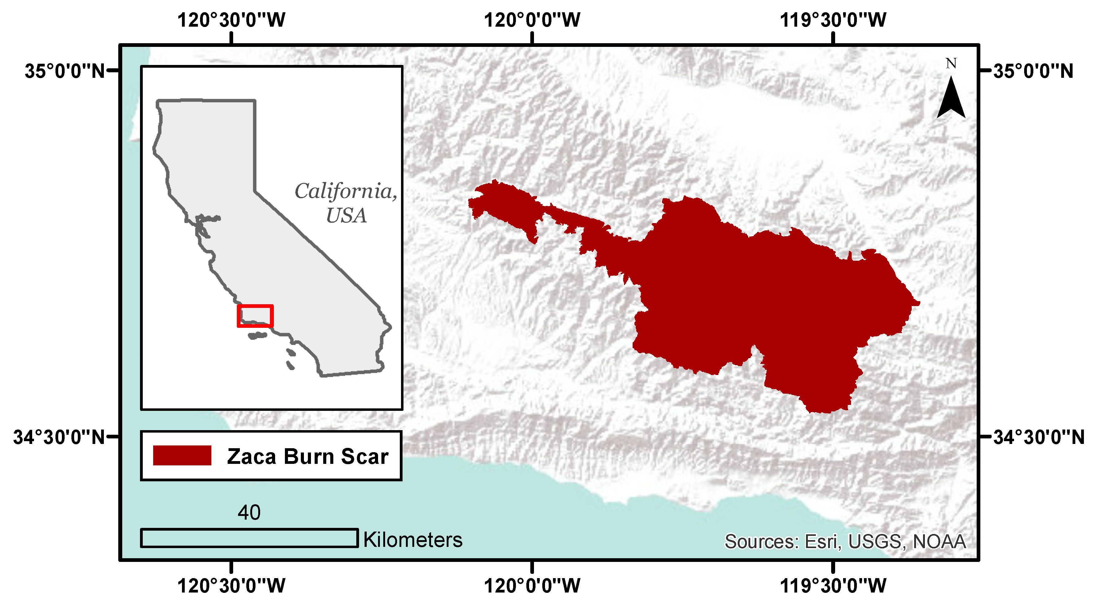
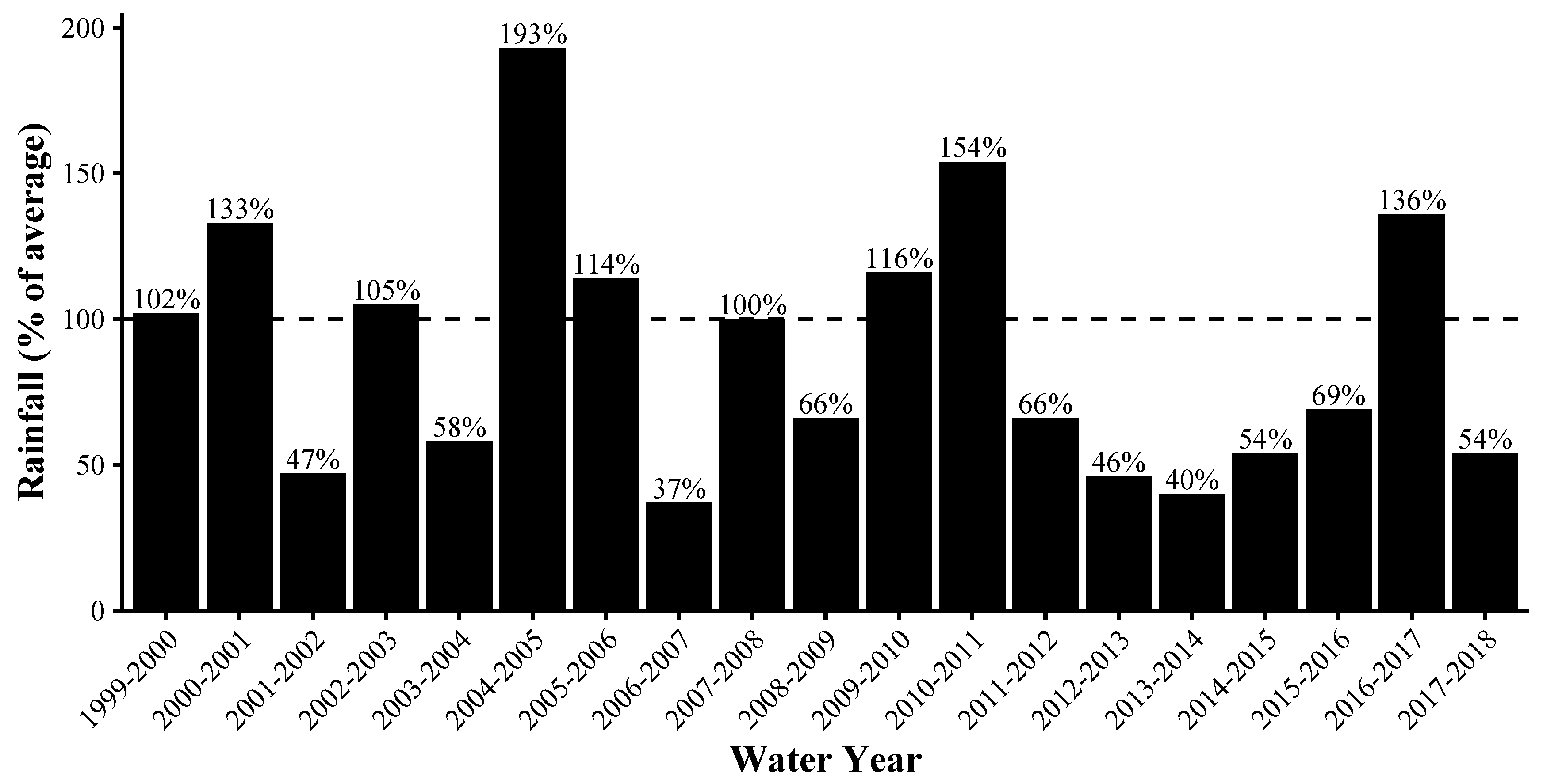
2.1. Study Area
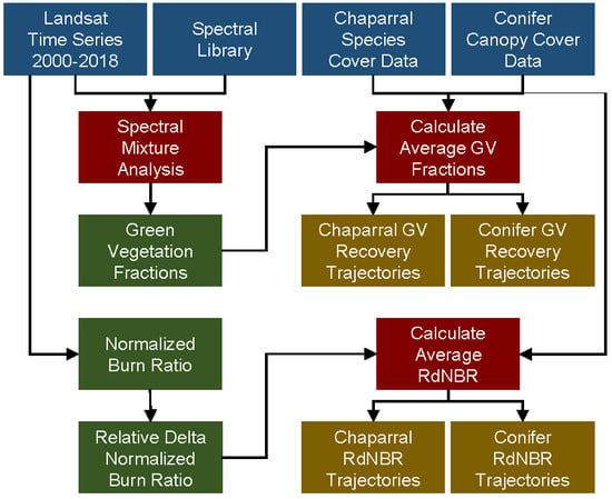
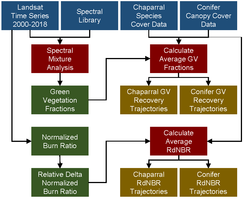
2.2. Remote Sensing
2.2.1. Imagery
2.2.2. Relative Delta Normalized Burn Ratio
2.2.3. Multiple Endmember Spectral Mixture Analysis
Spectral Library Development
- Ceanothus chaparral alliance
- Chamise alliance
- Scrub Oak alliance
- Coast Live Oak alliance
- Bigcone Douglas-fir alliance
- Black Cottonwood alliance
Spectral Unmixing
2.2.4. Assessment of Remote Sensing Products
2.3. Vegetation Field Surveys
- in an area of high burn severity (2007 dNBR > 600)
- homogenous vegetation composition
- homogenous slope and aspect
- minimum 40 m from a road to minimize the impacts of the road on surrounding vegetation (e.g., invasive grass)
- maximum 150 m from an accessible road or trail
- estimated slope less than 35 degrees
2.4. Conifer Canopy Cover
2.5. Recovery Trajectories
3. Results
3.1. Land Cover
3.2. Recovery Trajectories
3.2.1. Assessment of Remote Sensing Products
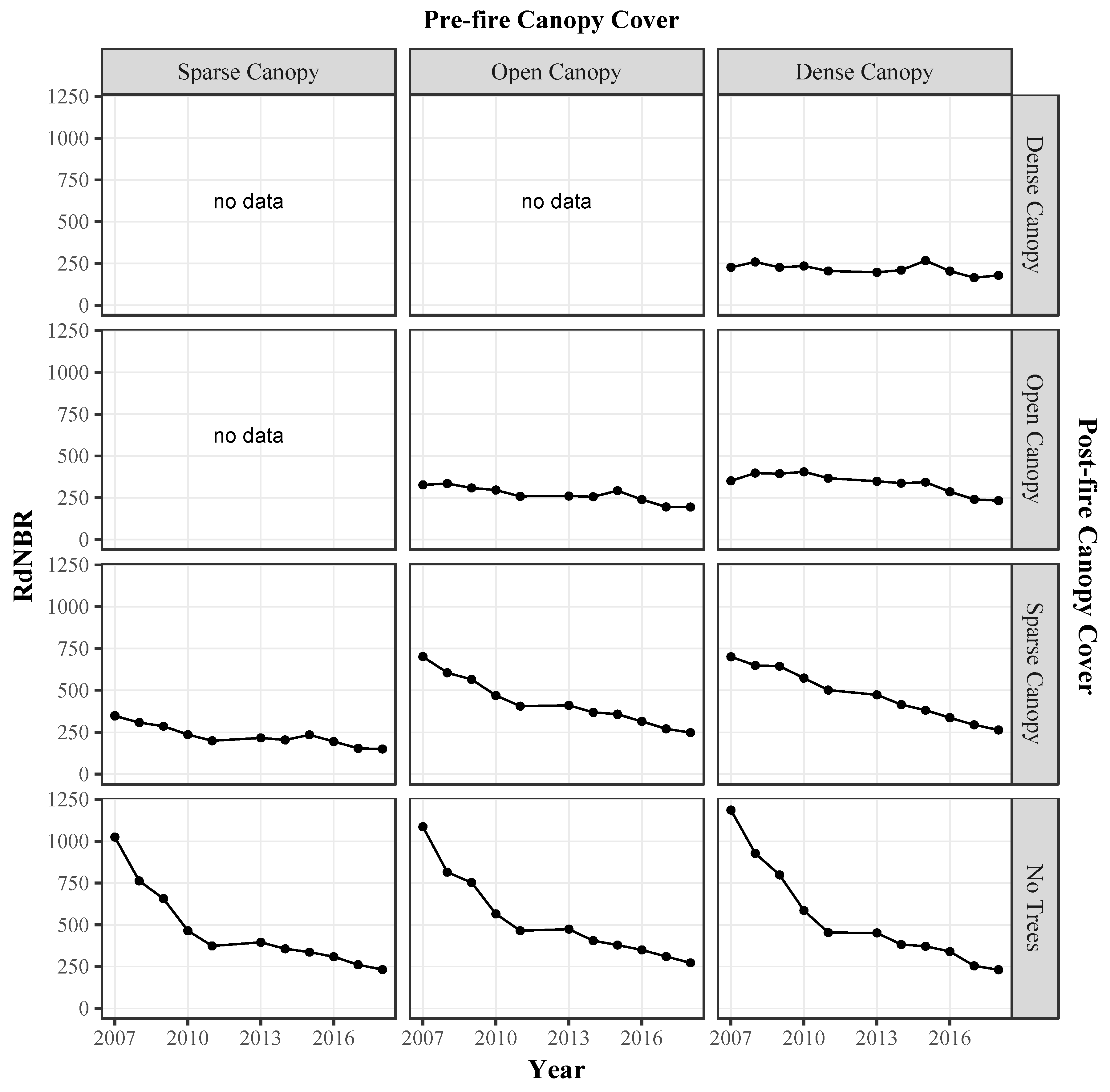
3.2.2. Relative Differenced Normalized Burn Ratio
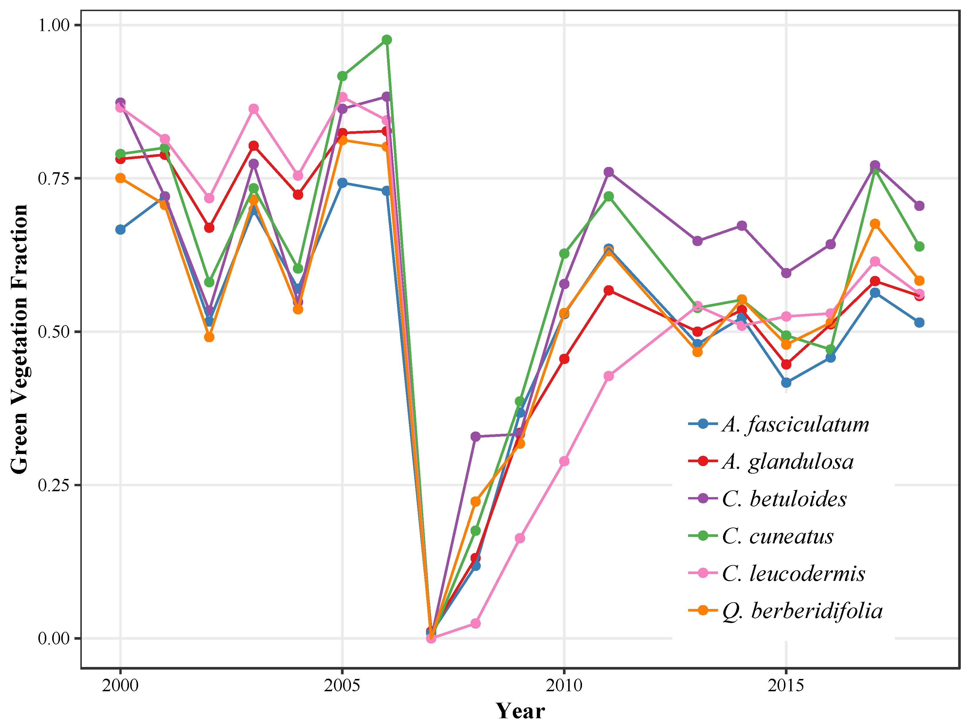
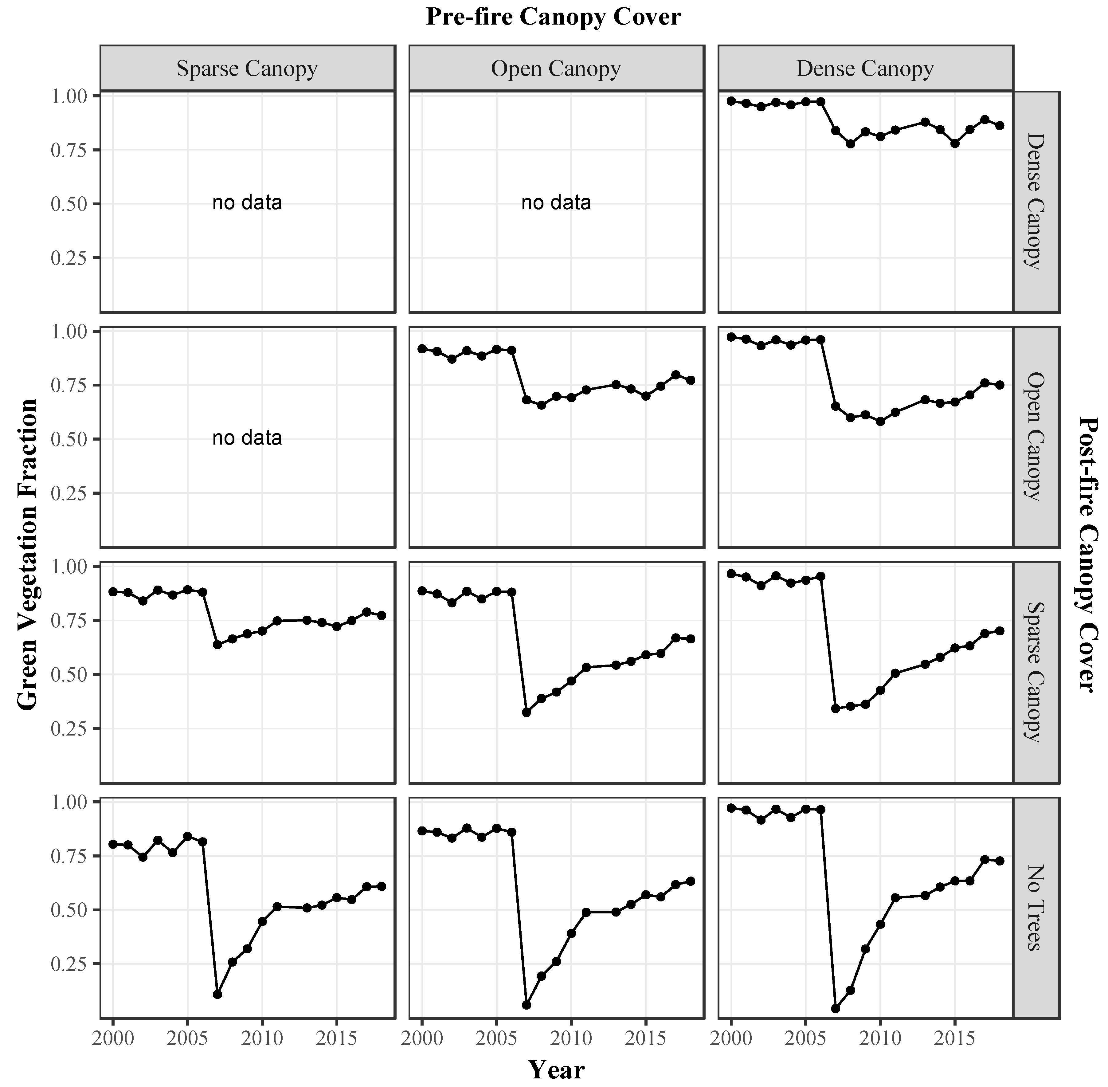
3.2.3. Green Vegetation Fractions
4. Discussion
4.1. Remote Sensing Products
4.2. Variability in Recovery Trajectories
4.2.1. Chaparral Species
4.2.2. Mixed Conifer Forest
4.3. Species Composition
4.4. Methodological Considerations
5. Conclusions
Author Contributions
Funding
Acknowledgments
Conflicts of Interest
References
- Keeley, J.E.; Brennan, T.; Pfaff, A.H. Fire severity and ecosystem responses following crown fires in California shrublands. Ecol. Appl. 2008, 18, 1530–1546. [Google Scholar] [CrossRef] [PubMed]
- Shakesby, R.; Doerr, S. Wildfire as a hydrological and geomorphological agent. Earth-Sci. Rev. 2006, 74, 269–307. [Google Scholar] [CrossRef]
- Coombs, J.S.; Melack, J.M. Initial impacts of a wildfire on hydrology and suspended sediment and nutrient export in California chaparral watersheds. Hydrol. Process. 2013, 27, 3842–3851. [Google Scholar] [CrossRef]
- Kashian, D.M.; Romme, W.H.; Tinker, D.B.; Turner, M.G.; Ryan, M.G. Carbon Storage on Landscapes with Stand-replacing Fires. BioScience 2006, 56, 598. [Google Scholar] [CrossRef]
- Gonzalez, P.; Battles, J.J.; Collins, B.M.; Robards, T.; Saah, D.S. Aboveground live carbon stock changes of California wildland ecosystems, 2001–2010. For. Ecol. Manag. 2015, 348, 68–77. [Google Scholar] [CrossRef]
- Jacobsen, A.L.; Pratt, R.B. Extensive drought-associated plant mortality as an agent of type-conversion in chaparral shrublands. New Phytol. 2018, 219, 498–504. [Google Scholar] [CrossRef] [Green Version]
- Dennison, P.E.; Brewer, S.C.; Arnold, J.D.; Moritz, M.A. Large wildfire trends in the western United States, 1984–2011. Geophys. Res. Lett. 2014, 41, 2928–2933. [Google Scholar] [CrossRef]
- Wulder, M.A.; Masek, J.G.; Cohen, W.B.; Loveland, T.R.; Woodcock, C.E. Opening the archive: How free data has enabled the science and monitoring promise of Landsat. Remote Sens. Environ. 2012, 122, 2–10. [Google Scholar] [CrossRef]
- Storey, E.A.; Stow, D.A.; O’Leary, J.F. Assessing postfire recovery of chamise chaparral using multi-temporal spectral vegetation index trajectories derived from Landsat imagery. Remote Sens. Environ. 2016, 183, 53–64. [Google Scholar] [CrossRef] [Green Version]
- Fernandez-Manso, A.; Quintano, C.; Roberts, D.A. Burn severity influence on post-fire vegetation cover resilience from Landsat MESMA fraction images time series in Mediterranean forest ecosystems. Remote Sens. Environ. 2016, 184, 112–123. [Google Scholar] [CrossRef]
- Frazier, R.J.; Coops, N.C.; Wulder, M.A.; Hermosilla, T.; White, J.C. Analyzing spatial and temporal variability in short-term rates of post-fire vegetation return from Landsat time series. Remote Sens. Environ. 2018, 205, 32–45. [Google Scholar] [CrossRef]
- Kennedy, R.E.; Yang, Z.; Cohen, W.B. Detecting trends in forest disturbance and recovery using yearly Landsat time series: 1. LandTrendr—Temporal segmentation algorithms. Remote Sens. Environ. 2010, 114, 2897–2910. [Google Scholar] [CrossRef]
- Key, C.H.; Benson, N.C. Landscape Assessment (LA). In FIREMON: Fire Effects Monitoring and Inventory System; Lutes, D.C., Ed.; U.S. Forest Service: Washington, DC, USA, 2006. [Google Scholar]
- Miller, J.D.; Thode, A.E. Quantifying burn severity in a heterogeneous landscape with a relative version of the delta Normalized Burn Ratio (dNBR). Remote Sens. Environ. 2007, 109, 66–80. [Google Scholar] [CrossRef]
- Hudak, A.T.; Morgan, P.; Bobbitt, M.J.; Smith, A.M.; Lewis, S.A.; Lentile, L.B.; Robichaud, P.R.; Clark, J.T.; McKinley, R.A. The Relationship of Multispectral Satellite Imagery to Immediate Fire Effects. Fire Ecol. 2007, 3, 64–90. [Google Scholar] [CrossRef]
- Rogan, J.; Franklin, J. Mapping Wildfire Burn Severity in Southern California Forests and Shrublands Using Enhanced Thematic Mapper Imagery. Geocarto Int. 2001, 16, 91–106. [Google Scholar] [CrossRef]
- Riaño, D.; Chuvieco, E.; Ustin, S.; Zomer, R.; Dennison, P.; Roberts, D.; Salas, J. Assessment of vegetation regeneration after fire through multitemporal analysis of AVIRIS images in the Santa Monica Mountains. Remote Sens. Environ. 2002, 79, 60–71. [Google Scholar] [CrossRef]
- Quintano, C.; Fernández-Manso, A.; Roberts, D.A. Multiple Endmember Spectral Mixture Analysis (MESMA) to map burn severity levels from Landsat images in Mediterranean countries. Remote Sens. Environ. 2013, 136, 76–88. [Google Scholar] [CrossRef]
- Key, C.H. Ecological and Sampling Constraints on Defining Landscape Fire Severity. Fire Ecol. 2006, 2, 34–59. [Google Scholar] [CrossRef]
- Rundel, P.W.; Parsons, D.J. Structural Changes in Chamise (Adenostoma fasciculatum) along a Fire-Induced Age Gradient. J. Range Manag. 1979, 32, 462. [Google Scholar] [CrossRef]
- Keeley, J.E.; Fotheringham, C.J.; Baer-Keeley, M. Determinants of postfire recovery and succession in Mediterranean-climate shrublands of California. Ecol. Appl. 2005, 15, 1515–1534. [Google Scholar] [CrossRef] [Green Version]
- Hope, A.; Tague, C.; Clark, R. Characterizing post-fire vegetation recovery of California chaparral using TM/ETM+ time-series data. Int. J. Remote Sens. 2007, 28, 1339–1354. [Google Scholar] [CrossRef]
- Röder, A.; Hill, J.; Duguy, B.; Alloza, J.; Vallejo, R. Using long time series of Landsat data to monitor fire events and post-fire dynamics and identify driving factors. A case study in the Ayora region (eastern Spain). Remote Sens. Environ. 2008, 112, 259–273. [Google Scholar] [CrossRef]
- Davis, F.W.; Michaelsen, J. Sensitivity of fire regime in chaparral ecosystems to climate change. In Global Change and Mediterranean-Type Ecosystems; Moreno, J.M., Oechel, W.C., Eds.; Springer: New York, NY, USA, 1995. [Google Scholar]
- Baldwin, B.G.; Goldman, D.H.; Keil, D.J.; Patterson, R.; Rosatti, T.J.; Wilken, D.H. The Jepson Manual: Vascular Plants of California, 2nd ed.; University of California Press: Berkeley, CA, USA, 2012. [Google Scholar]
- Santa Barbara County Public Works Department. County-Wide Percent-of-Normal Water-Year Rainfall. Available online: https://www.countyofsb.org/uploadedFiles/pwd/Content/Water/Hydrology/Rainfall%20-%20Annual%20Percent%20of%20Normal%20-%20CountyWide.pdf (accessed on 13 November 2019).
- Griffin, D.; Anchukaitis, K.J. How unusual is the 2012-2014 California drought? Geophys. Res. Lett. 2014, 41, 9017–9023. [Google Scholar] [CrossRef] [Green Version]
- Robeson, S.M. Revisiting the recent California drought as an extreme value. Geophys. Res. Lett. 2015, 42, 6771–6779. [Google Scholar] [CrossRef]
- Wang, S.Y.S.; Yoon, J.H.; Becker, E.; Gillies, R. California from drought to deluge. Nat. Clim. Chang. 2017, 7, 465–468. [Google Scholar] [CrossRef]
- National Drought Mitigation Center, U.S. Department of Agriculture, and National Oceanic and Atmospheric Association. United States Drought Monitor. Available online: https://droughtmonitor.unl.edu (accessed on 13 November 2019).
- Markham, B.; Storey, J.; Williams, D.; Irons, J. Landsat sensor performance: history and current status. IEEE Trans. Geosci. Remote Sens. 2004, 42, 2691–2694. [Google Scholar] [CrossRef]
- Masek, J.; Vermote, E.; Saleous, N.; Wolfe, R.; Hall, F.; Huemmrich, K.; Gao, F.; Kutler, J.; Lim, T.K. A Landsat Surface Reflectance Dataset for North America, 1990–2000. IEEE Geosci. Remote Sens. Lett. 2006, 3, 68–72. [Google Scholar] [CrossRef]
- California Department of Department of Forestry and Fire Protection. Fire Perimeters. Available online: https://frap.fire.ca.gov/mapping/gis-data (accessed on 1 December 2017).
- Green, R.O.; Eastwood, M.L.; Sarture, C.M.; Chrien, T.G.; Aronsson, M.; Chippendale, B.J.; Faust, J.A.; Pavri, B.E.; Chovit, C.J.; Solis, M.; et al. Imaging Spectroscopy and the Airborne Visible/Infrared Imaging Spectrometer (AVIRIS). Remote Sens. Environ. 1998, 65, 227–248. [Google Scholar] [CrossRef]
- Lee, C.M.; Cable, M.L.; Hook, S.J.; Green, R.O.; Ustin, S.L.; Mandl, D.J.; Middleton, E.M. An introduction to the NASA Hyperspectral InfraRed Imager (HyspIRI) mission and preparatory activities. Remote Sens. Environ. 2015, 167, 6–19. [Google Scholar] [CrossRef]
- Thompson, D.R.; Gao, B.C.; Green, R.O.; Roberts, D.A.; Dennison, P.E.; Lundeen, S.R. Atmospheric correction for global mapping spectroscopy: ATREM advances for the HyspIRI preparatory campaign. Remote Sens. Environ. 2015, 167, 64–77. [Google Scholar] [CrossRef]
- Meerdink, S.K.; Roberts, D.A.; Roth, K.L.; King, J.Y.; Gader, P.D.; Koltunov, A. Classifying California plant species temporally using airborne hyperspectral imagery. Remote Sens. Environ. 2019, 232, 111308. [Google Scholar] [CrossRef]
- Miller, J.D.; Knapp, E.E.; Key, C.H.; Skinner, C.N.; Isbell, C.J.; Creasy, R.M.; Sherlock, J.W. Calibration and validation of the relative differenced Normalized Burn Ratio (RdNBR) to three measures of fire severity in the Sierra Nevada and Klamath Mountains, California, USA. Remote Sens. Environ. 2009, 113, 645–656. [Google Scholar] [CrossRef]
- Hubbert, K.R.; Wohlgemuth, P.M.; Beyers, J.L.; Narog, M.G.; Gerrard, R. Post-Fire Soil Water Repellency, Hydrologic Response, and Sediment Yield Compared between Grass-Converted and Chaparral Watersheds. Fire Ecol. 2012, 8, 143–162. [Google Scholar] [CrossRef]
- Roberts, D.; Smith, M.; Adams, J. Green vegetation, nonphotosynthetic vegetation, and soils in AVIRIS data. Remote Sens. Environ. 1993, 44, 255–269. [Google Scholar] [CrossRef]
- Smith, M.O.; Ustin, S.L.; Adams, J.B.; Gillespie, A.R. Vegetation in deserts: I. A regional measure of abundance from multispectral images. Remote Sens. Environ. 1990, 31, 1–26. [Google Scholar] [CrossRef]
- Roberts, D.A.; Ustin, S.L.; Ogunjemiyo, S.; Greenberg, J.; Dobrowski, S.Z.; Chen, J.; Hinckley, T.M. Spectral and Structural Measures of Northwest Forest Vegetation at Leaf to Landscape Scales. Ecosystems 2004, 7. [Google Scholar] [CrossRef]
- Roberts, D.; Gardner, M.; Church, R.; Ustin, S.; Scheer, G.; Green, R. Mapping Chaparral in the Santa Monica Mountains Using Multiple Endmember Spectral Mixture Models. Remote Sens. Environ. 1998, 65, 267–279. [Google Scholar] [CrossRef]
- Roth, K.L.; Dennison, P.E.; Roberts, D.A. Comparing endmember selection techniques for accurate mapping of plant species and land cover using imaging spectrometer data. Remote Sens. Environ. 2012, 127, 139–152. [Google Scholar] [CrossRef]
- Zare, A.; Ho, K. Endmember Variability in Hyperspectral Analysis. IEEE Signal Process. Mag. 2013, 31, 95–104. [Google Scholar] [CrossRef]
- Tane, Z.; Roberts, D.; Veraverbeke, S.; Casas, R.; Ramirez, C.; Ustin, S. Evaluating Endmember and Band Selection Techniques for Multiple Endmember Spectral Mixture Analysis using Post-Fire Imaging Spectroscopy. Remote Sens. 2018, 10, 389. [Google Scholar] [CrossRef] [Green Version]
- Tompkins, S.; Mustard, J.F.; Pieters, C.M.; Forsyth, D.W. Optimization of endmembers for spectral mixture analysis. Remote Sens. Environ. 1997, 59, 472–489. [Google Scholar] [CrossRef]
- Somers, B.; Asner, G.P.; Tits, L.; Coppin, P. Endmember variability in Spectral Mixture Analysis: A review. Remote Sens. Environ. 2011, 115, 1603–1616. [Google Scholar] [CrossRef]
- Asner, G.P.; Heidebrecht, K.B. Spectral unmixing of vegetation, soil and dry carbon cover in arid regions: Comparing multispectral and hyperspectral observations. Int. J. Remote Sens. 2002, 23, 3939–3958. [Google Scholar] [CrossRef]
- U.S. Forest Service, Pacific Southwest Region. Existing Vegetation—CALVEG. Available online: https://www.fs.usda.gov/detail/r5/landmanagement/resourcemanagement/?cid=stelprdb5347192 (accessed on 1 May 2018).
- Schaaf, A.N.; Dennison, P.E.; Fryer, G.K.; Roth, K.L.; Roberts, D.A. Mapping Plant Functional Types at Multiple Spatial Resolutions Using Imaging Spectrometer Data. Gisci. Remote Sens. 2011, 48, 324–344. [Google Scholar] [CrossRef]
- Bodí, M.B.; Martin, D.A.; Balfour, V.N.; Santín, C.; Doerr, S.H.; Pereira, P.; Cerdà, A.; Mataix-Solera, J. Wildland fire ash: Production, composition and eco-hydro-geomorphic effects. Earth Sci. Rev. 2014, 130, 103–127. [Google Scholar] [CrossRef]
- Roberts, D.A.; Batista, G.T.; Pereira, J.L.; Waller, E.K.; Nelson, B.W. Change Identification Using Multitemporal Spectral Mixture Analysis: Applications in Eastern Amazonia. In Remote Sensing Change Detection: Environmental Monitoring Methods and Applications; Ann Arbor Press: Chelsea, MI, USA, 1998; pp. 137–161. [Google Scholar]
- Powell, R.; Roberts, D.; Dennison, P.; Hess, L. Sub-pixel mapping of urban land cover using multiple endmember spectral mixture analysis: Manaus, Brazil. Remote Sens. Environ. 2007, 106, 253–267. [Google Scholar] [CrossRef]
- Roberts, D.A.; Halligan, K.; Dennison, P.; Dudley, K.; Somers, B.; Crabbé, A. VIPER Tools User Manual Version 2.1; University of California: Santa Barbara, CA, USA, 2019. [Google Scholar]
- Roberts, D.; Dennison, P.; Gardner, M.; Hetzel, Y.; Ustin, S.; Lee, C. Evaluation of the potential of hyperion for fire danger assessment by comparison to the airborne visible/infrared imaging spectrometer. IEEE Trans. Geosci. Remote Sens. 2003, 41, 1297–1310. [Google Scholar] [CrossRef]
- Liu, N.; Treitz, P. Modelling high arctic percent vegetation cover using field digital images and high resolution satellite data. Int. J. Appl. Earth Obs. Geoinf. 2016, 52, 445–456. [Google Scholar] [CrossRef]
- Liu, N. Photo Grid Classifier. Software. Python code available from author. University of Wisconsin-Madison.
- Jennings, M.D.; Faber-Langendoen, D.; Loucks, O.L.; Peet, R.K.; Roberts, D. Standards for associations and alliances of the U.S. National Vegetation Classification. Ecol. Monogr. 2009, 79, 173–199. [Google Scholar] [CrossRef]
- Powell, R.; Matzke, N.; de Souza, C.; Clark, M.; Numata, I.; Hess, L.; Roberts, D. Sources of error in accuracy assessment of thematic land-cover maps in the Brazilian Amazon. Remote Sens. Environ. 2004, 90, 221–234. [Google Scholar] [CrossRef]
- Canada’s National Forest Inventory. Photo Plot Data Dictionary for Second Remeasurement; Natural Resources Canada: Victoria, BC, Canada, 2017. [Google Scholar]
- Stenback, J.M.; Congalton, R.G. Using Thematic Mapper Imagery to Examine Forest Understory. Photogramm. Eng. Remote Sens. 1990, 56, 1285–1290. [Google Scholar]
- Borchert, M.; Lopez, A.; Bauer, C.; Knowd, T. Field Guide to Coastal Sage Scrub and Chaparral Alliances of Los Padres National Forest; Number R5-TP-019; U.S. Forest Service: Washington, DC, USA, 2004.
- Keeley, J.E.; Davis, F.W. Chaparral. In Terrestrial Vegetation of California, 3rd ed.; University of California Press: Berkeley, CA, USA, 2007; pp. 339–366. [Google Scholar]
- Venturas, M.D.; MacKinnon, E.D.; Dario, H.L.; Jacobsen, A.L.; Pratt, R.B.; Davis, S.D. Chaparral Shrub Hydraulic Traits, Size, and Life History Types Relate to Species Mortality during California’s Historic Drought of 2014. PLoS ONE 2016, 11, e0159145. [Google Scholar] [CrossRef] [PubMed] [Green Version]
- Keeley, J.E. Seed Production, Seed Populations in Soil, and Seedling Production After Fire for Two Congeneric Pairs of Sprouting and Nonsprouting Chaparal Shrubs. Ecology 1977, 58, 820–829. [Google Scholar] [CrossRef]
- Vogl, R.J.; Schorr, P. Fire and Manzanita Chaparral in the San Jacinto Mountains, California. Ecology 1972, 53, 1179–1188. [Google Scholar] [CrossRef]
- Keeley, J.E. Recruitment of Seedlings and Vegetative Sprouts in Unburned Chaparral. Ecology 1992, 73, 1194–1208. [Google Scholar] [CrossRef]
- Keeley, J.E. Fire Severity and Plant Age in Postfire Resprouting of Woody Plants in Sage Scrub and Chaparral. Madroño 2006, 53, 373–379. [Google Scholar] [CrossRef]
- Swain, D.L.; Langenbrunner, B.; Neelin, J.D.; Hall, A. Increasing precipitation volatility in twenty-first-century California. Nat. Clim. Chang. 2018, 8, 427–433. [Google Scholar] [CrossRef]
- Frolking, S.; Palace, M.W.; Clark, D.B.; Chambers, J.Q.; Shugart, H.H.; Hurtt, G.C. Forest disturbance and recovery: A general review in the context of spaceborne remote sensing of impacts on aboveground biomass and canopy structure. J. Geophys. Res. Biogeosci. 2009, 114. [Google Scholar] [CrossRef]
- Keeley, J.E. Fire intensity, fire severity and burn severity: A brief review and suggested usage. Int. J. Wildland Fire 2009, 18, 116. [Google Scholar] [CrossRef]
- Foody, G.M.; Boyd, D.S.; Cutler, M.E. Predictive relations of tropical forest biomass from Landsat TM data and their transferability between regions. Remote Sens. Environ. 2003, 85, 463–474. [Google Scholar] [CrossRef]
- Morresi, D.; Vitali, A.; Urbinati, C.; Garbarino, M. Forest Spectral Recovery and Regeneration Dynamics in Stand-Replacing Wildfires of Central Apennines Derived from Landsat Time Series. Remote Sens. 2019, 11, 308. [Google Scholar] [CrossRef] [Green Version]
- Horton, J.S.; Kraebel, C.J. Development of Vegetation after Fire in the Chamise Chaparral of Southern California. Ecology 1955, 36, 244–262. [Google Scholar] [CrossRef]
- Williams, J.E.; Davis, S.D.; Portwood, K. Xylem Embolism in Seedlings and Resprouts of Adenostoma fasciculatum after Fire. Aust. J. Bot. 1997, 45, 291. [Google Scholar] [CrossRef]
- Paddock, W.; Davis, S.; Pratt, B.; Jacobsen, A.; Tobin, M.; López-Portillo, J.; Ewers, F. Factors Determining Mortality of Adult Chaparral Shrubs in an Extreme Drought Year in California. Aliso 2013, 31, 49–57. [Google Scholar] [CrossRef] [Green Version]
- Schwilk, D.W.; Ackerly, D.D. Is there a cost to resprouting? Seedling growth rate and drought tolerance in sprouting and nonsprouting Ceanothus (Rhamnaceae). Am. J. Bot. 2005, 92, 404–410. [Google Scholar] [CrossRef] [Green Version]
- Jacobsen, A.L.; Pratt, R.B.; Ewers, F.W.; Davis, S.D. Cavitation Resistance among 26 Chaparral Species of Southern California. Ecol. Monogr. 2007, 77, 99–115. [Google Scholar] [CrossRef]
- Meentemeyer, R.K.; Moody, A. Distribution of plant life history types in California chaparral: the role of topographically-determined drought severity. J. Veg. Sci. 2002, 13, 67. [Google Scholar] [CrossRef]
- Peterson, S.H.; Stow, D.A. Using multiple image endmember spectral mixture analysis to study chaparral regrowth in southern California. Int. J. Remote Sens. 2003, 24, 4481–4504. [Google Scholar] [CrossRef]
- McMichael, C.E.; Hope, A.S.; Roberts, D.A.; Anaya, M.R. Post-fire recovery of leaf area index in California chaparral: A remote sensing-chronosequence approach. Int. J. Remote Sens. 2004, 25, 4743–4760. [Google Scholar] [CrossRef]
- Kane, V.R.; Lutz, J.A.; Roberts, S.L.; Smith, D.F.; McGaughey, R.J.; Povak, N.A.; Brooks, M.L. Landscape-scale effects of fire severity on mixed-conifer and red fir forest structure in Yosemite National Park. For. Ecol. Manag. 2013, 287, 17–31. [Google Scholar] [CrossRef]
- Franklin, J. Thematic mapper analysis of coniferous forest structure and composition. Int. J. Remote Sens. 1986, 7, 1287–1301. [Google Scholar] [CrossRef]
- Minnich, R.A.; Goforth, B.R.; Paine, T.D. Follow the Water: Extreme Drought and the Conifer Forest Pandemic of 2002–2003 Along the California Borderland. In Insects and Diseases of Mediterranean Forest Systems; Paine, T.D., Ed.; Springer: New York, NY, USA, 2015; pp. 859–890. [Google Scholar]
- Harvey, B.J.; Donato, D.C.; Turner, M.G. High and dry: post-fire tree seedling establishment in subalpine forests decreases with post-fire drought and large stand-replacing burn patches: Drought and post-fire tree seedlings. Glob. Ecol. Biogeogr. 2016, 25, 655–669. [Google Scholar] [CrossRef] [Green Version]
- Stevens-Rumann, C.S.; Kemp, K.B.; Higuera, P.E.; Harvey, B.J.; Rother, M.T.; Donato, D.C.; Morgan, P.; Veblen, T.T. Evidence for declining forest resilience to wildfires under climate change. Ecol. Lett. 2018, 21, 243–252. [Google Scholar] [CrossRef] [PubMed]
- DeFries, R.S.; Field, C.B.; Fung, I.; Justice, C.O.; Los, S.; Matson, P.A.; Matthews, E.; Mooney, H.A.; Potter, C.S.; Prentice, K.; et al. Mapping the land surface for global atmosphere-biosphere models: Toward continuous distributions of vegetation’s functional properties. J. Geophys. Res. 1995, 100, 20867. [Google Scholar] [CrossRef]
- Lambin, E.F. Monitoring forest degradation in tropical regions by remote sensing: Some methodological issues. Glob. Ecol. Biogeogr. 1999, 8, 191–198. [Google Scholar] [CrossRef]
- Kennedy, R.E.; Andréfouët, S.; Cohen, W.B.; Gómez, C.; Griffiths, P.; Hais, M.; Healey, S.P.; Helmer, E.H.; Hostert, P.; Lyons, M.B.; et al. Bringing an ecological view of change to Landsat-based remote sensing. Front. Ecol. Environ. 2014, 12, 339–346. [Google Scholar] [CrossRef]
- Abatzoglou, J.T.; Williams, A.P. Impact of anthropogenic climate change on wildfire across western US forests. Proc. Natl. Acad. Sci. USA 2016, 113, 11770–11775. [Google Scholar] [CrossRef] [Green Version]


| Species | Compositional Similarity (%) | Dominant Species Cover (%) | Number of Transects |
|---|---|---|---|
| Adenostoma fasciculatum | 60.84 | 40.18 | 19 |
| Arctostaphylos glandulosa | 56.34 | 32.53 | 15 |
| Ceanothus cuneatus | 54.67 | 47.94 | 7 |
| Ceanothus leucodermis | 58.74 | 35.27 | 7 |
| Ceanothus oliganthus | 62.41 | 52.94 | 4 |
| Ceanothus palmeri | 54.04 | 40.79 | 5 |
| Cercocarpus betuloides | 73.49 | 30.16 | 2 |
| Hosackia crassifolia | 82.96 | 39.64 | 2 |
| Quercus berberidifolia | 54.27 | 40.15 | 12 |
| Quercus chrysolepis | 51.39 | 36.94 | 5 |
| Quercus wislizenii | 51.80 | 30.56 | 4 |
| Grass spp. | 57.19 | 35.53 | 5 |
© 2019 by the authors. Licensee MDPI, Basel, Switzerland. This article is an open access article distributed under the terms and conditions of the Creative Commons Attribution (CC BY) license (http://creativecommons.org/licenses/by/4.0/).
Share and Cite
Kibler, C.L.; Parkinson, A.-M.L.; Peterson, S.H.; Roberts, D.A.; D’Antonio, C.M.; Meerdink, S.K.; Sweeney, S.H. Monitoring Post-Fire Recovery of Chaparral and Conifer Species Using Field Surveys and Landsat Time Series. Remote Sens. 2019, 11, 2963. https://0-doi-org.brum.beds.ac.uk/10.3390/rs11242963
Kibler CL, Parkinson A-ML, Peterson SH, Roberts DA, D’Antonio CM, Meerdink SK, Sweeney SH. Monitoring Post-Fire Recovery of Chaparral and Conifer Species Using Field Surveys and Landsat Time Series. Remote Sensing. 2019; 11(24):2963. https://0-doi-org.brum.beds.ac.uk/10.3390/rs11242963
Chicago/Turabian StyleKibler, Christopher L., Anne-Marie L. Parkinson, Seth H. Peterson, Dar A. Roberts, Carla M. D’Antonio, Susan K. Meerdink, and Stuart H. Sweeney. 2019. "Monitoring Post-Fire Recovery of Chaparral and Conifer Species Using Field Surveys and Landsat Time Series" Remote Sensing 11, no. 24: 2963. https://0-doi-org.brum.beds.ac.uk/10.3390/rs11242963