An End-to-End Local-Global-Fusion Feature Extraction Network for Remote Sensing Image Scene Classification


Research Institute of information Fusion, Naval Aviation University, Yantai 264001, China
*
Author to whom correspondence should be addressed.
Remote Sens. 2019, 11(24), 3006; https://0-doi-org.brum.beds.ac.uk/10.3390/rs11243006
Submission received: 8 November 2019
/
Revised: 6 December 2019
/
Accepted: 10 December 2019
/
Published: 13 December 2019
(This article belongs to the Special Issue Feature-Based Methods for Remote Sensing Image Classification)
Abstract
:Remote sensing image scene classification (RSISC) is an active task in the remote sensing community and has attracted great attention due to its wide applications. Recently, the deep convolutional neural networks (CNNs)-based methods have witnessed a remarkable breakthrough in performance of remote sensing image scene classification. However, the problem that the feature representation is not discriminative enough still exists, which is mainly caused by the characteristic of inter-class similarity and intra-class diversity. In this paper, we propose an efficient end-to-end local-global-fusion feature extraction (LGFFE) network for a more discriminative feature representation. Specifically, global and local features are extracted from channel and spatial dimensions respectively, based on a high-level feature map from deep CNNs. For the local features, a novel recurrent neural network (RNN)-based attention module is first proposed to capture the spatial layout information and context information across different regions. Gated recurrent units (GRUs) is then exploited to generate the important weight of each region by taking a sequence of features from image patches as input. A reweighed regional feature representation can be obtained by focusing on the key region. Then, the final feature representation can be acquired by fusing the local and global features. The whole process of feature extraction and feature fusion can be trained in an end-to-end manner. Finally, extensive experiments have been conducted on four public and widely used datasets and experimental results show that our method LGFFE outperforms baseline methods and achieves state-of-the-art results.
1. Introduction
Rapid technological advancement and development of instruments for earth observation are responsible for the generation of numerous high-resolution remote sensing images. Consequently, there has been a surge in demand for effective understanding of the semantic content and accurate identification and classification of land use and land cover scenes [1,2,3]. Remote sensing image scene classification (RSISC) focuses on categorizing acquired images into the pre-defined classes according to the semantic content of scene images, which has been extensively explored due to the important role it plays in many applications.
As an active topic of the remote sensing area, RSISC has received growing attention and numerous methods have been proposed to solve this task. Especially from the proposal of AlexNet [4] for classifying the dataset ImageNet containing 1000 categories and more than one million natural images, deep learning-based methods have been proven to have a better performance and show superior potential compared to handcrafted features-based ones [5,6]. The success of deep learning-based methods is mainly attributed to the stacking of a variety of convolutional layers with non-linearity, which can extract more high-level semantic information, thereby helping to alleviate the problem of semantic gap.
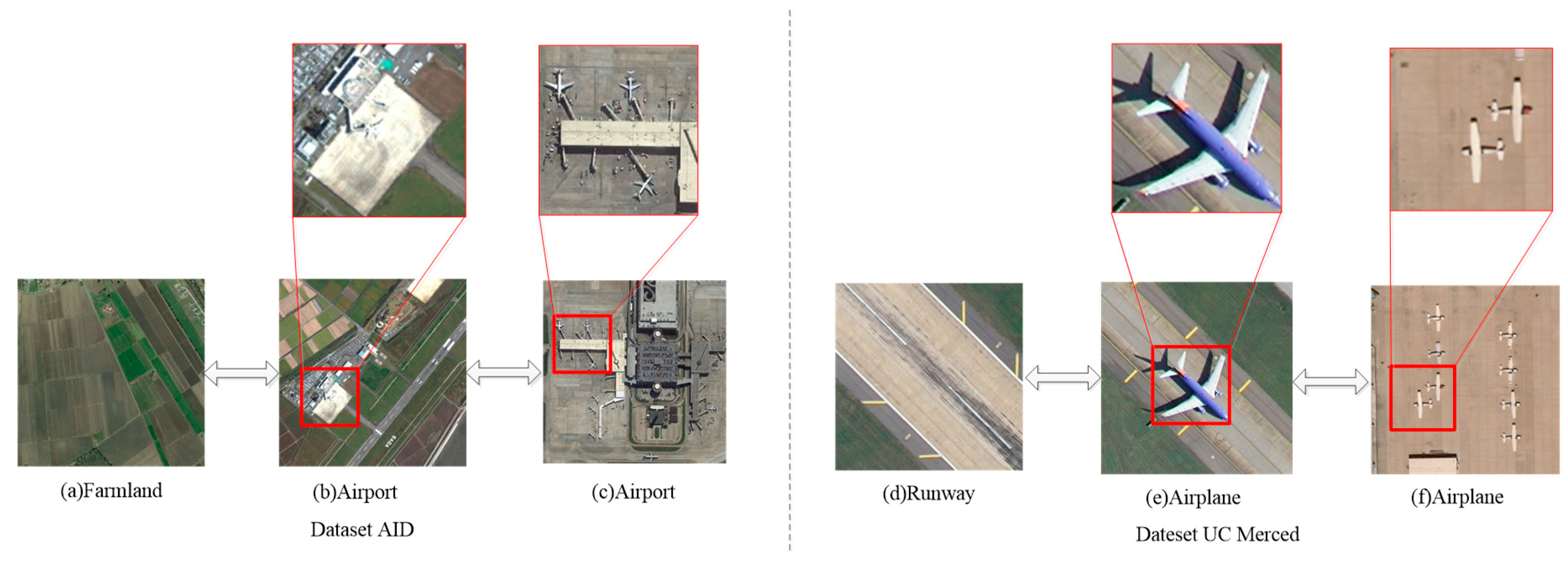
Deep learning-based methods have exhibited remarkably better performance in computer vision [4,7,8,9]. However, RSISC is still a big challenge for the large differences between natural and remote sensing images, as well as inapplicability of the deep learning-based methods in representing remote sensing images. Particularly, remote sensing images are more complex than natural ones, which cover a large area from the “view of God”, contain many types of contents and objects, and their semantics are very ambiguous [10]. As some samples for the task of RSISC shown in Figure 1, there are some images from different categories sharing many similar contents and semantics, such as the farmland in Figure 1a,b, and the runway in Figure 1d,e. Whereas some scene images from the same category may show high diversity in content, such as the Figure 1b,c and the Figure 1e,f. Furthermore, the terms of semantic categories (e.g., farmland and airport) summarily describe the content of scene images in high-level abstraction [10], and some attributes (e.g., the farmland in Figure 1b and the runway in Figure 1e) in the scene images are not fully described by the category labels. Such inter-class similarity and intra-class diversity introduce higher requirements for the discriminative ability of feature representation with many solutions now being proposed to generate more discriminative feature representations to tackle this problem. For instance, Reference [11] proposes a discriminative-CNN (D-CNN) model by imposing a metric learning regularization term on convolutional neural networks (CNNs) features, such that image features from the same category are pulled closer and the features belonging to different categories are pushed away in the feature space. A multi-scale CNN framework is proposed in Reference [12] to extract the scale-invariant features from multiscale input images and deal with the problem of intra-class diversity caused by scale variation of the objects, such as the airplane in Figure 1e,f. To deal with the issue of the same semantic class being observed in arbitrary orientations in remote sensing images, a rotation-equivariant and rotation-invariant network has been proposed [13,14] to realize the rotation equivariance and rotation invariance in the CNNs itself.
Although these methods can improve the discriminative ability of feature representation for the task of RSISC, they only adopt the global features while ignoring some key local features. As shown in Figure 1, the key to correctly distinguishing the different categories with similar global features and identifying the same categories with different global features is the local region in the red box. Some methods have, therefore, been proposed to further exploit the local features. For instance, Reference [15] proposes a region-wise deep feature extraction framework to extract the regions that may contain the target information firstly, and extract and encode the regional features by the pretrained convolutional neural networks (CNNs) and vector of locally aggregated descriptors (VLAD) to generate the final feature representation. A method to rearrange the local features is proposed in Reference [16] by comparing the similarity between every local feature of image patch and their corresponding center image after a clustering with the global features. In addition, a recurrent attention structure is demonstrated in Reference [17] to generate a series of mask matrices that have the same size with high-level features to reweigh the importance of every element in high-level features respectively, and a long short-term memory (LSTM)-based sequential processor is adopted to process and fuse the series of attention representation. These methods make use of local features to some extent, although some limitations still exist. For instance, the region-wise deep network [15] only extracts and combines the local features and discards the global features. The rearranging local features proposed in Reference [16] cannot be trained end-to-end. The process of rearranging is complex and computationally intensive. The attention recurrent convolutional network in Reference [17] can be trained end-to-end, but the attention map is generated to reweigh the importance of every element in the high-level feature map, and not different regions.
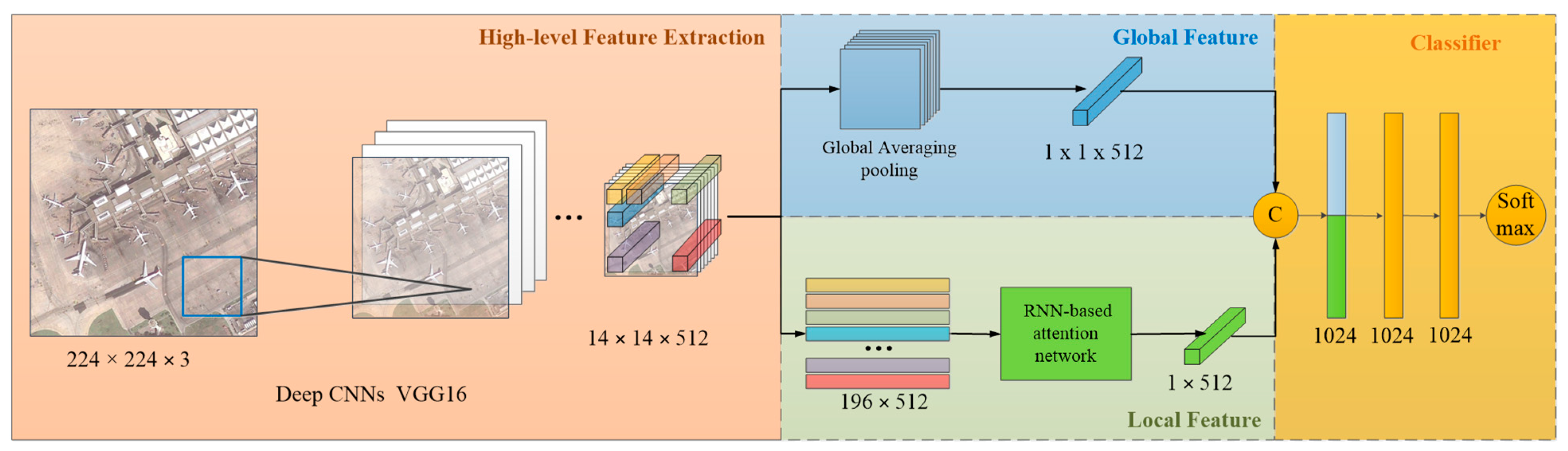
Based on the above discussions and aforementioned limitations, this paper proposes an end-to-end local-global-fusion feature extraction (LGFFE) network for RSISC, as shown in Figure 2. Based on the high-level feature map extracted by deep CNNs, the local and global features can be obtained from the dimension of channel and spatial, respectively. A novel recurrent neural network (RNN)-based attention module is proposed to generate discriminative local features, which can capture the regional features and context information of different regions and reweigh the importance of different image regions. A sequence of image patches’ features are taken as input, with a selective focus on key regions as well as suppression of the noncritical ones. Then, the local features are fused with global features extracted from the high-level features to perform as the final feature representation. Our main contributions can be summarized as follows.
We propose a novel end-to-end LGFFE network which can extract global and local features based on the high-level features and further fuse them to acquire a more discriminative feature representation for remote sensing images.
We design an efficient RNN-based attention module to capture the context information and extract discriminative local features, which takes a sequence of image regions’ features as input and generates the importance weight of every region through the gated recurrent units (GRUs) network with attention mechanism.
Extensive experiments have been conducted on four widely used, but differently characterized, datasets to demonstrate the effectiveness of our method. Results from these experiments show that our LGFFE module outperforms most existing baselines and achieves state-of-the-art results.
The rest of the paper is organized as follows. Section 2 presents some published work related to remote sensing image scene classification. Our proposed method is introduced in Section 3, and Section 4 displays detailed experimental results and analyses. Section 5 includes a discussion and Section 6 draws some conclusions.
2. Related Work
In this section, we will present some related work on remote sensing image scene classification, three kinds of methods on feature representation are introduced, and some discriminative feature representation methods for remote sensing image are introduced.
2.1. Remote Sensing Image Scene Classification
In the last decades, RSISC has been widely studied for its broad applications. Visual descriptors and a classifier are usually combined to solve the problem of scene classification. The discriminative ability of feature embedding plays an important role in the construction of an effective scene classification method. Based on the types of features used in scene classification, existing methods can be divided into three categories: low-level, middle-level, and high-level feature-based methods. Early works for RSISC are mainly based on low-level features, designed by exploiting engineering skills and domain expertise to acquire hand-crafted features. These included global features, color [18], texture [19,20], shape [21], as well as local features based on scale-invariant feature transform (SIFT) [22] and speeded up robust feature (SURF) [23]. However, performance of low-level features is constrained by the existing “semantic gap” between insufficient discriminative ability of the low-level features and high-level semantic information of remote sensing scene images. To counter this problem, middle-level features have been developed to encode the local features to get a holistic representation. The bag-of-visual-words (BoVW) [24] is one of the most commonly used middle-level features. It first extracts local image features by local descriptors, then generates the codebook by clustering, and finally acquires the visual word histogram to determine their category. Moreover, other middle-level features have also been proposed to consider the semantic information based on BoVW, such as latent dirichlet allocation (LDA) [25] and probabilistic latent semantic analysis (pLSA) [26,27]. Recently, deep learning-based methods have been dominant in many computer vision tasks, such as classification, detection, and retrieval. Deep learning-based methods have also achieved impressive results and state-of-the-art performance in RSISC [5,28]. Their effectiveness can be attributed to deep and non-linear networks and the ability to extract the high-level semantic information. Pre-trained CNNs [29,30], fine-tuned CNNs [31,32], and a combination of CNNs and local feature methods [33] are three main types of high-level features used in RSISC. Despite great progress achieved by these deep learning-based methods in RSISC, there still exists some inapplicability for remote sensing images. Compared to natural images, remote sensing images have some special characteristics, including scale ambiguity, category ambiguity, and rotation ambiguity [34], which make them difficult to be correctly represented by the deep CNNs used for natural images.
2.2. Discriminative Feature Representation for Remote Sensing
Recently, many solutions, for obtaining a more discriminative feature representation, have been explored. One of the most effective ones involves an attention mechanism, which has been proven to be effective in tasks including visual attention [35,36] and textual attention [37,38]. Here, an attention structure is proposed in Reference [17] to generate several attention representations based on the high-level features, which is the first use of attention mechanism in remote sensing. While the method in Reference [17] generates an attention mask for each element in the high-level feature map, Reference [39] proposes a new attention module to emphasize the meaningful features along the channel and spatial dimensions based on the high-level features. The effectiveness of this attention module has subsequently been verified in the task of remote sensing image retrieval. At the same time, the attention mechanism can focus on important regions to solve the problem of large width of remote sensing images. Feature fusion is another important solution to the feature representation. A novel feature fusion framework has been proposed in Reference [33] to fuse the low-level, middle-level, and high-level features, and the global and local features. During this fusion, two fusion approaches, the fully connected features and the pooling-stretched convolutional features, are proposed to fuse the local and global features. Discriminant correlation analysis (DCA) is also introduced in Reference [40] as a strategy to fuse and refine deep features from a pretrained visual geometry group network (VGG). Different full-connected layers in the VGG are regarded as different features and first combined. Apart from this, other new frameworks are introduced for a discriminative feature. For instance, metric learning is adopted in Reference [11] to supervise the learning of deep CNNs by optimizing a new discriminative objective function, to ensure that images belonging to the same class are mapped closely while those from different categories are as far apart as possible. The multi-scale CNN is proposed in Reference [12] to solve the problem of scale ambiguity of remote sensing images, in which the fixed scale and carried-scale nets are contained to train the multi-scale images.
3. The Proposed Approach
This section mainly details our proposed global-local-fusion method, including high-level features extraction, global and local features extraction in Section 3.1 and Section 3.2, and some further analysis to local features extraction module in Section 3.3.
The framework of our proposed method is shown in Figure 2. First, high-level features are extracted by the deep CNNs and the VGG16 [8] is taken as an example in this section. Input images are resized to 224 × 224 and fed into the VGG16 for the global and local features, as shown in the framework. The last convolutional layer of VGG16, with a size of 14 × 14 × 512, is adopted as the basic high-level features. Based on the high-level features, the global and local features can be acquired from channel and spatial dimensions, respectively.
3.1. Global Feature Extraction from Channel Dimension
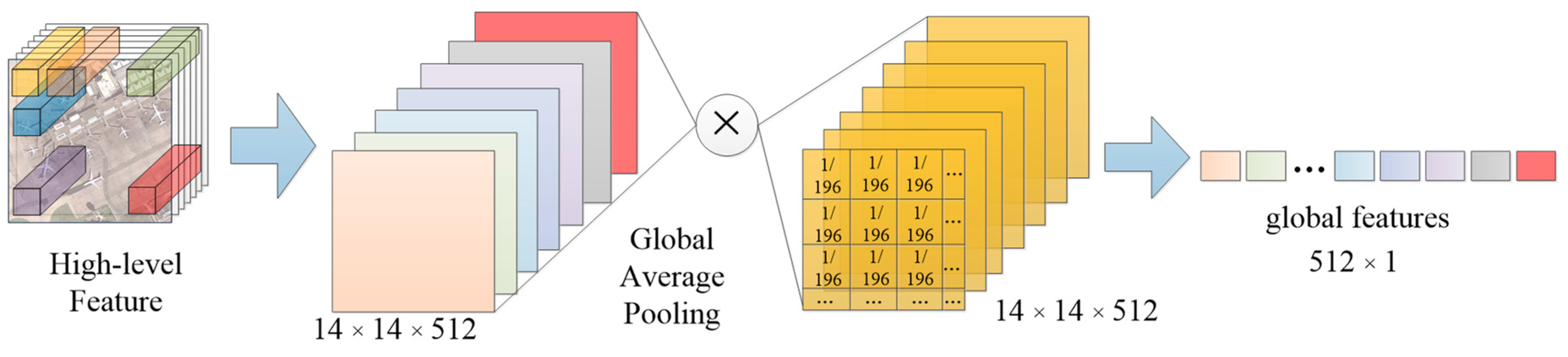
Global features play an important role in the image representation and the task of classification. These features should contain the general information of an image. For the high-level feature, acquired from deep CNNs, the channel’s number is 512, which is equal to the number of filters in the last convolutional layer. Generally, more high-level semantic information contained in the last convolutional layer of deep CNNs is usually treated as the feature representation of the input image, while each filter in the convolution operation can be regard as an extraction of a certain feature. Therefore, the high-level feature, , in channel dimensions can be thought of as a collection of different features. In our global feature extraction module, global average pooling is adopted to get each channel’s average value as representation of that kind of feature. The resulting 512-dimensional feature vector is regarded as the global feature representation, , as shown in Figure 3 and Equation (1).
where denotes the channel in high-level feature with a total number of 512, the is the average matrix with a size of 14 × 14 and each pixel in is set as 1/196, the denotes the operation of element-wise multiplication.
3.2. Local Feature Extraction from Spatial Dimension
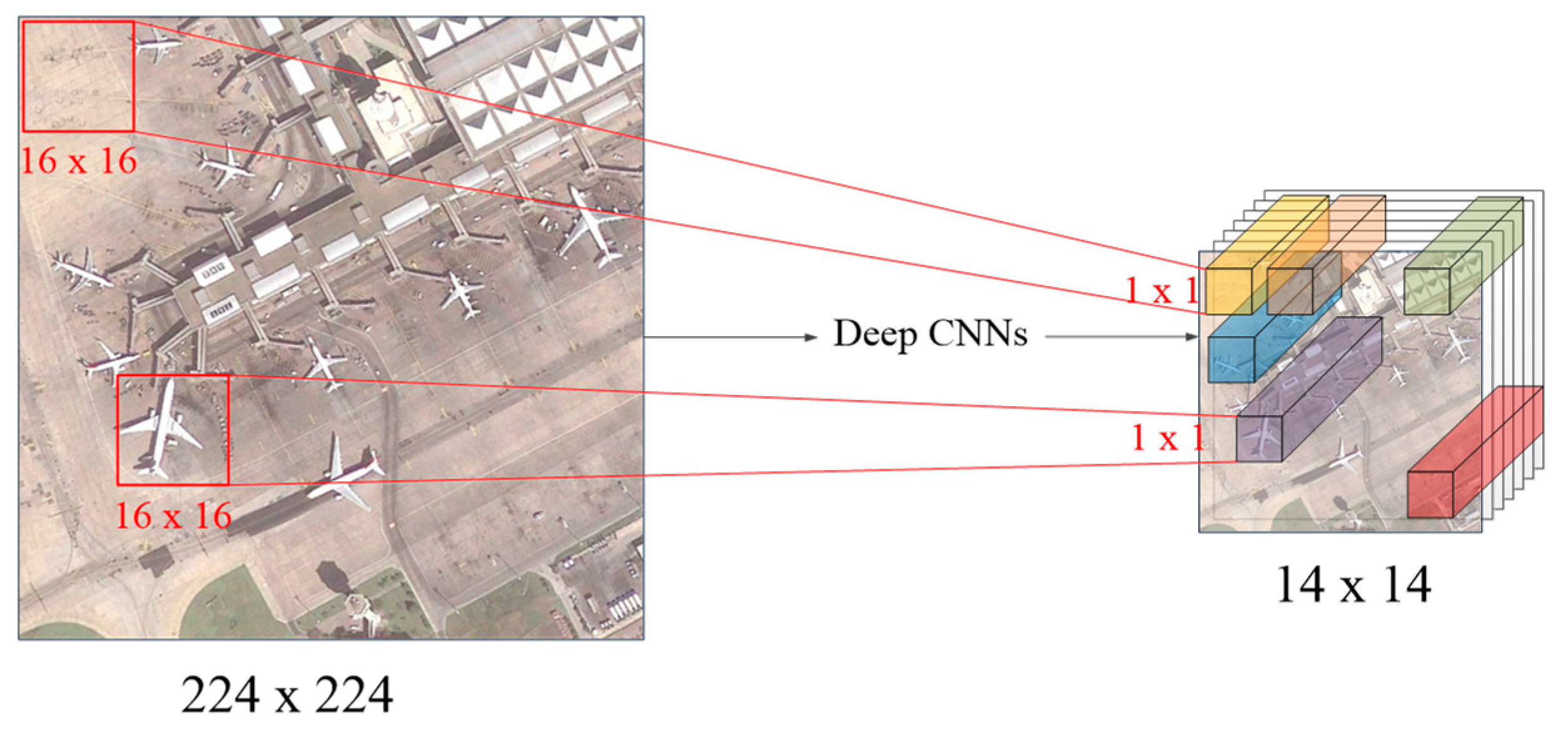
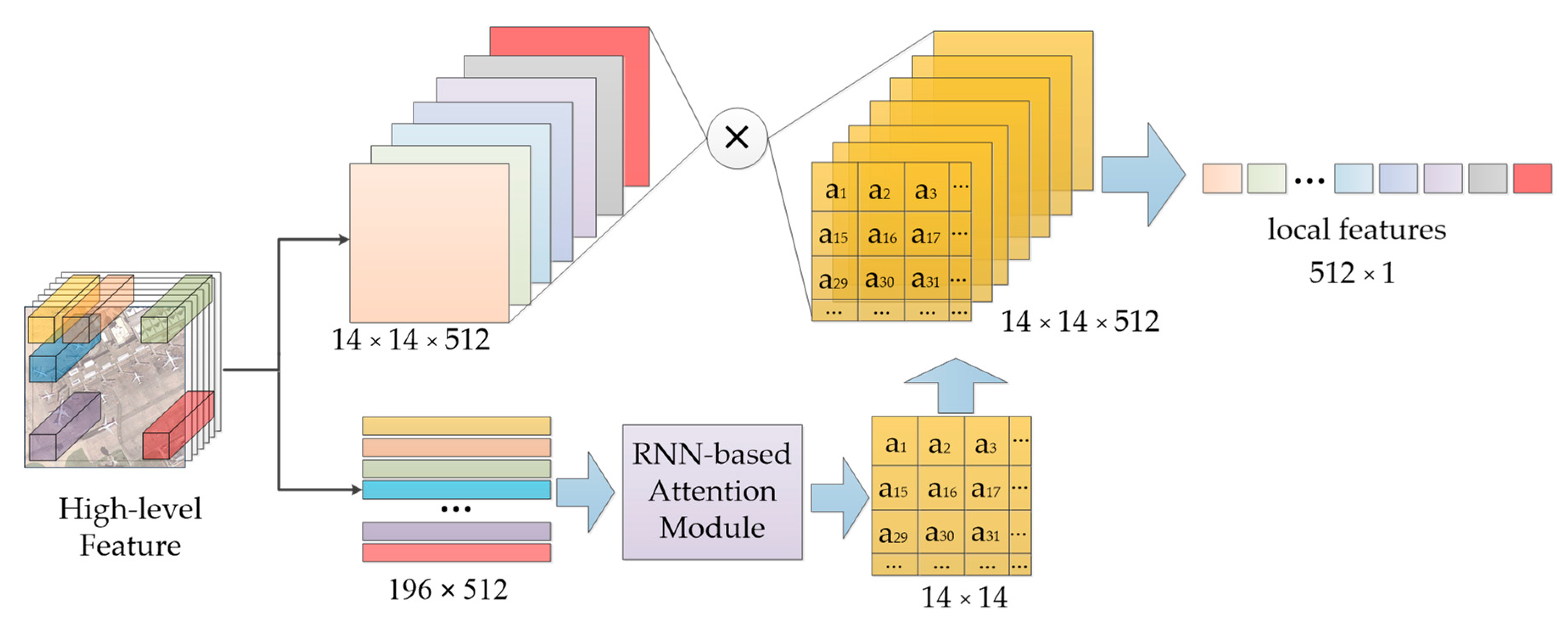
Compared to global feature, a local feature should focus on the information of silent regions in the image to further improve discriminative ability. The original image is usually divided into small image blocks, then used for extracting local features, which may be the usual pipeline of local feature extraction, such as the proposed multi-patch pooling [41]. In our method, an end-to-end local feature extraction framework is proposed and combined with the global feature extraction module, based on the high-level feature of deep CNNs. As shown in Figure 4, the image size drops from 224 × 224 to 14 × 14 through the pooling operation in CNNs. Every pixel (1 × 1) in high-level feature corresponds to the original image block with the size of 16 × 16. The vector of 1 × 1 × 512 in the high-level feature can, therefore, be treated as the regional feature with the original size of 16 × 16. Based on the above analysis, we take the sequence of local high-level feature as an input and design an RNN-based local feature extraction module with attention mechanism to model the local features and spatial context information. With this, a reweighed weight mask is learned to reweigh the importance of different image blocks.
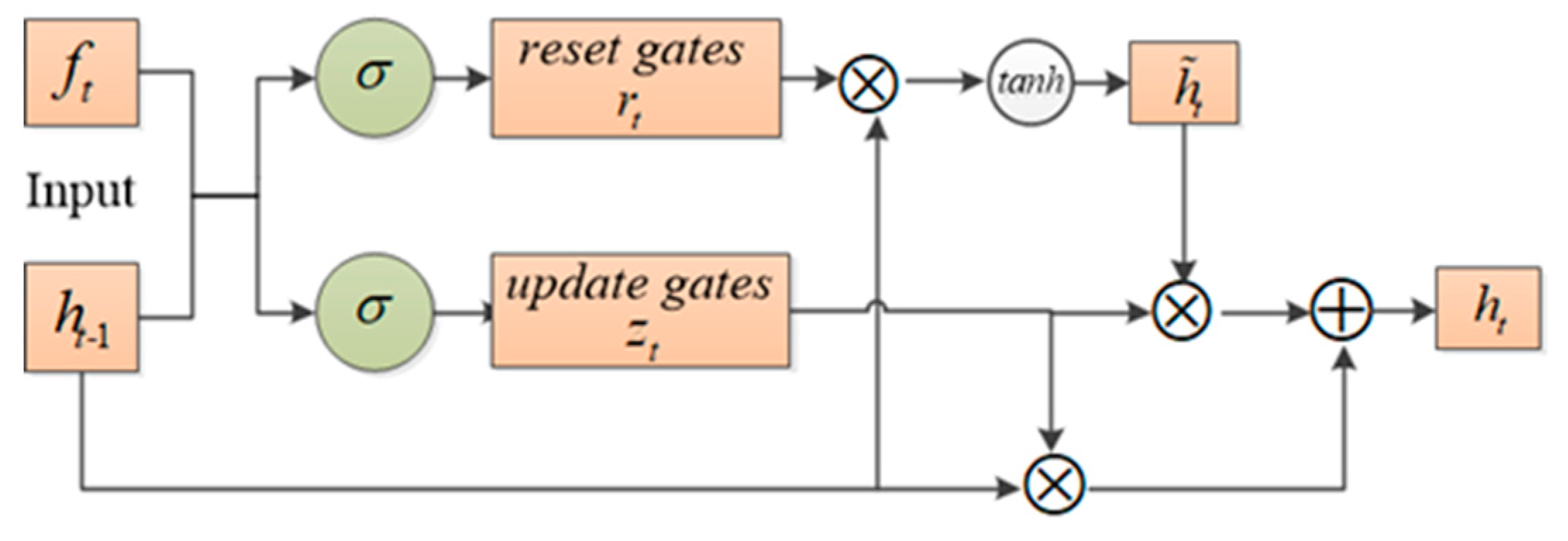
From the high-level features, we can acquire 196 vectors, which are the original feature representations of different regions, and can be represented as . Based on the results of our eye moving when we scan an image [42], we treat these regional features as a sequence and enter them orderly into RNN, from left to right, then top to bottom. Gated recurrent units (GRUs) [43], a special kind of RNN with fewer parameters and better performance [44,45], is adopted to learn the long-term dependencies and preserve previous information in the image sequence by the update gates and reset gates . Given the input and , the updates of GRU are as follows:
where, denotes the sigmoid function, is the element-wise multiplication, and its architecture is shown in Figure 5.
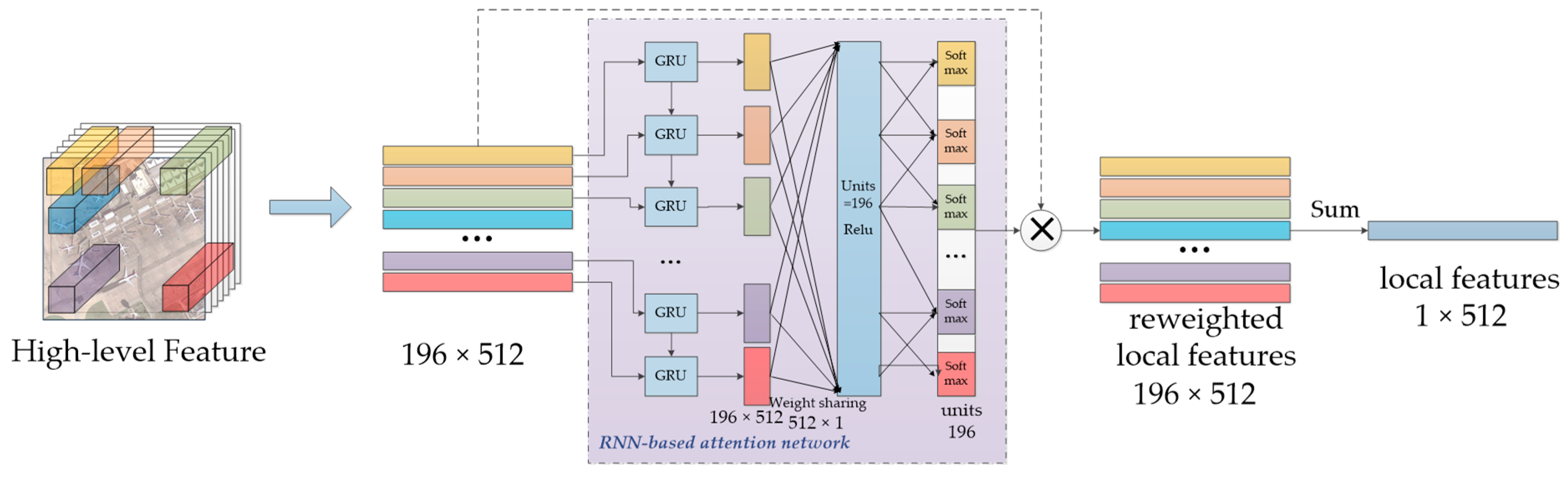
After that, we construct an RNN-based attention module with time step t = 196, as shown in Figure 6, with regional features as inputs. Output sequences from GRU can be acquired and regarded as the revised local feature representation by considering the context information of different image blocks. Then, to calculate the regional features’ attention weights, , two fully-connected (FC) networks with activation functions are connected to further revise the weights, as shown in the following equations:
where the first FC layer is a weight-sharing layer. The size of weight matrix is set to 512 × 1 to map the input regional feature of 512-dimension to 1-dimension, while the acquired 512 values of every region are concatenated and connected with the next FC layer. The second FC layer has 512 output units with the weight matrix to output the reweighted importance of different regions. With the attention weight A, the reweighted regional features , and local features can be obtained as,
3.3. Further Analysis to Local Feature Extraction Module
The motivation of the local feature extraction module is generating an attention weight, A, to reweight the importance of different regions. The reweighted regional features are summed together to acquire the final feature representation, as shown in Equation (9). Concretely, this computing process in Equation (9) can be conducted in another way to explain the process of local feature extraction. The input in Equation (9) is the regional feature in high-level feature , which can be represented as . Consequently, the Equation (9) can be represented as:
where , while denotes the element-wise multiplication.
From the final results shown in Equation (10), we can find that it has a similar structure to Equation (1). However, the main difference is that the average weight matrix in Equation (1) is replaced by the revised weight matrix A. Based on the above analysis, the local feature extraction module can be regarded as a new method for global pooling. Global average pooling and global max pooling are the two main pooling ways to acquire the representation of channels by the global average value and global max value. This kind of pooling method, however, totally neglects the spatial information in the channel. Conversely, our local feature extraction module takes full consideration of spatial information to focus on the silent regions by an attention-based weight matrix, as shown in Figure 7.
To combine the general and regional information, we fuse the global and local features to obtain a final feature representation. As shown in Figure 2, concatenation is adopted to fuse the local and global information to acquire a local-global-fusion feature. Then, the multi-layer perceptron (MLP) composed of two fully connected layers and batch normalization layers is designed as the classifier to classify the local-global-fusion feature. Finally, cross-entropy loss function is adopted as the loss function.
4. Experiments and Analysis
4.1. Datasets Description
In order to evaluate the performance of our method, four public datasets, UC Merced Land-Use dataset (UCM) [24], Aerial Image dataset (AID) [46], NWPU-RESISC45 dataset (NWPU45) [47], and OPTIMAL-31 dataset [17], designed for remote sensing image scene classification, are used in our experiments.
The UCM dataset is a widely used dataset for the task of remote sensing image scene classification. It consists of 2100 images and as well as 21 land-use categories, including airplane, agricultural, baseball diamond, buildings, beach, chaparral, dense residential, freeway, forest, golf course, harbor, intersection, mobile home park, medium density residential, overpass, parking lot, runway, river, storage tanks, sparse residential, and tennis courts. Each of these classes contains 100 images with a size of 256 × 256 pixels and a 30 cm resolution.
The AID is a large-scale dataset for the task of scene classification. It is collected from Google Earth and consists of 10,000 images with a size of 600 × 600 pixels. This dataset is divided into the following 30 categories: airport, bare land, beach, baseball field, bridge, center, commercial, church, dense residential, desert, forest, farmland, industrial, meadow, mountain, medium residential, parking, park, port, playground, pond, railway station, river, resort, school, stadium, sparse residential, storage tanks, square, and viaduct. The number of images in each category varies from 220 to 420, while the spatial resolution ranges from half a meter to 8 m.
The NWPU45 is a more challenging dataset for the task of scene classification, owing to a larger scale on the total number of images and scene categories. This dataset is also acquired from Google Earth and covers more than 100 countries. It consists of 31,500 remote sensing images and the following 45 scene classes, airport, airplane, basketball court, baseball diamond, beach, bridge, church, chaparral, circular farmland, commercial area, cloud, dense residential, desert, forest, freeway, ground track field, golf course, harbor, industrial area, island, intersection, lake, meadow, medium residential, mountain, mobile home park, overpass, palace, parking lot, railway station, railway, roundabout, rectangular farmland, river, runway, sea ice, snowberg, ship, sparse residential, storage tank, stadium, tennis court, thermal power station, terrace, and wetland. Each category contains 700 images with a size of 256 × 256 and a spatial resolution ranging from about 0.2 to 30 m per pixel.
OPTIMAL-31 is a new dataset for RSISC constructed in Reference [17]. The dataset contains 31 categories, each category comprising 60 images with a size of 256 × 256. These categories include: airplane, airport, basketball court, baseball field, bridge, beach, bushes, crossroads, church, round farmland, business district, desert, harbor, dense houses, factory, forest, freeway, golf field, island, lake, meadow, medium houses, mountain, mobile house area, overpass, playground, parking lot, roundabout, runway, railway, and square farmland. OPTIMAL-31 has been a more challenge dataset for the task of RSISC, due to a high number of categories and less images contained in each category. Therefore, we suppose it is useful for testing the generalization performance of the classification model.
4.2. Experimental Setup
In this section, some experiment details, including dataset setting, evaluation metrics, and some important parameters, will be illustrated.
(1) Dataset setting: For the dataset UCM, we randomly select 80% of the images of each class for training while the remaining 20% are used for testing. We split the images in dataset AID into 50%, 20% for training and 50%, 80% for testing. For NWPU45, the training ratio of images number is set to 10%, 20%, and the rest 90%, 80% is for testing. 80% of images per category are selected for training in OPTIMAL-31, and the remaining 20% for testing. These settings are the same as the works in References [12,17,33,46] for an ease of comparison in performances.
(2) Evaluation metrics: For the task of remote sensing image scene classification, overall accuracy (OA) and confusion matrix (CM) are the most widely used evaluation metrics for evaluating the classification results. The OA is equal to the number of correctly classified images, divided by the number of total testing images, regardless of the category information. This is a general and direct measure for showing classification performance. On the other hand, CM is a more detailed table for the visualization of the performance between all classes. The CM is acquired by counting the correct number of classified images in each category in the test set. Each element in the matrix is the proportion of images predicted to be the n-th categories and actually belonging to the m-th category. We repeat every experiment 10 times for each training set, and the mean and standard deviation of the experimental results will be reported.
(3) Training parameters: For the high-level feature extraction, we adopt the pre-trained CNNs to finetune on the remote sensing images. We set the batch size to 64 and learning rate to 5e-4. The experiment is implemented based on Keras with two NVIDIA GTX 1080Ti GPU for acceleration. During testing, the penultimate fully connected layer is treated as the final feature representation of image, and a liner support vector machine (SVM) rather than the softmax function used during training, is adopted as the classifier. SVM could get a better performance compared to the MLP under the same condition, and this has been verified in some works [11,30]. The detailed parameters and the code of our LGFFE are available at https://pan.baidu.com/s/1jk3BF3qPcHrUO92s7orfow, with password “85jf”.
(4) High-level feature extractor: Our local-global-fusion feature extractor (LGFFE) can be applied to any deep CNNs. Because various CNNs may generate different features, we have tested several baseline CNNs as the high-level feature extractors to identify a better one. The VGG16, VGG19 [8] and ResNet50 [7] are chosen to acquire the last convolutional layer as our high-level feature. A comparison of different CNNs combined with our local-global-fusion feature extraction module on the dataset AID is shown in Table 1. It can be found that ResNet50 combined with our LGFFE have a better performance than VGG16 and VGG19, and ResNet50 is chosen as our high-level feature extractor in our following experiments.
4.3. Experimental Results and Comparisons
In this section, extensive experiments on four public datasets are conducted and reported to show the effectiveness of our method. According to the description in Section 4.1, there are large differences in data categories, data volumes, and resolution among these four datasets, which are useful aspects for verifying the generalization and applicability of our methods.
4.3.1. Experiment 1: UC Merced Land-Use (UCM) Dataset
The dataset UCM is the most widely used remote sensing scene classification dataset. The performance of our method in comparison with some state-of-the-art methods on the dataset UCM is shown in Table 2. Although many methods have tested on UCM, only the deep CNNs-based methods, with superior performance to handcrafted features, are used for comparisons here.
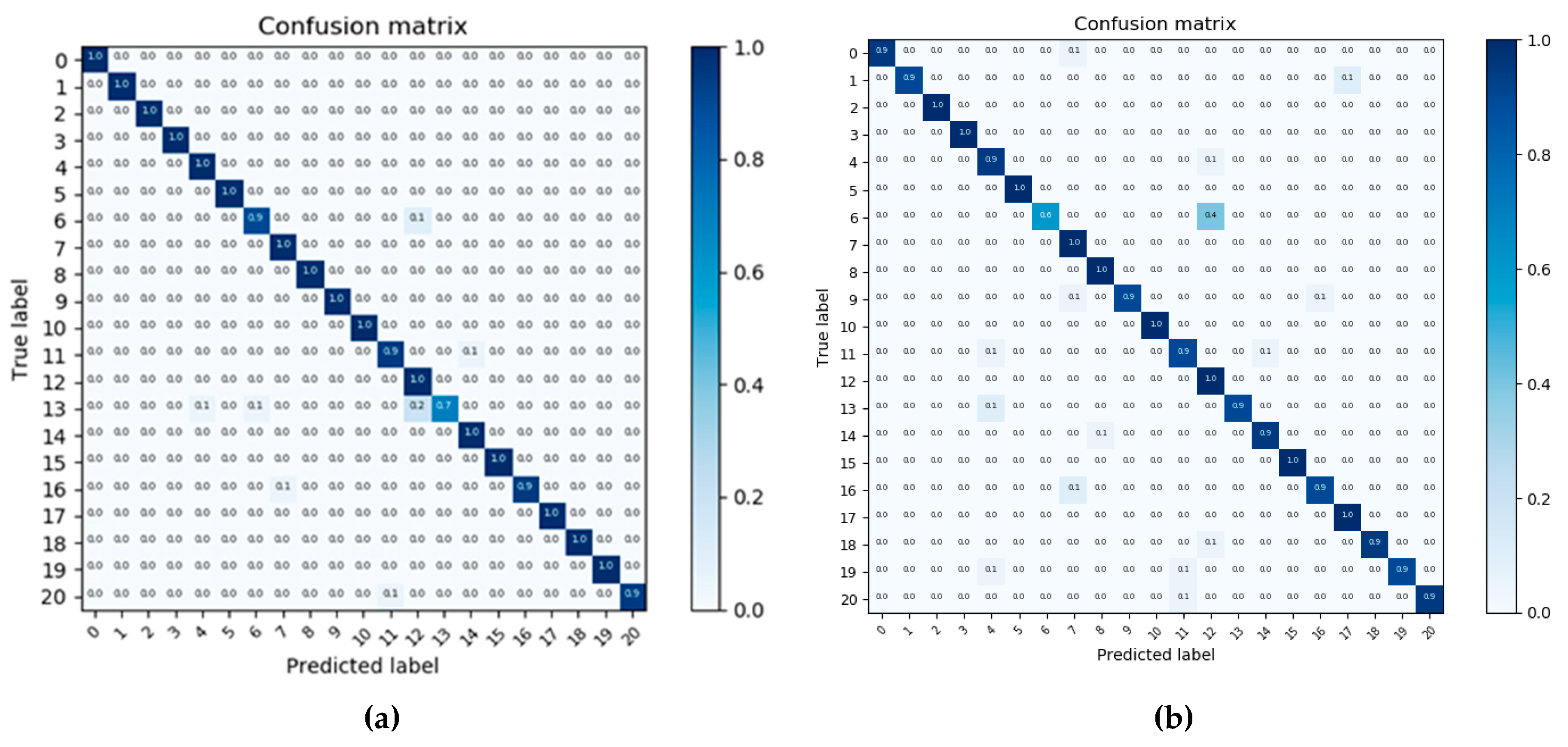
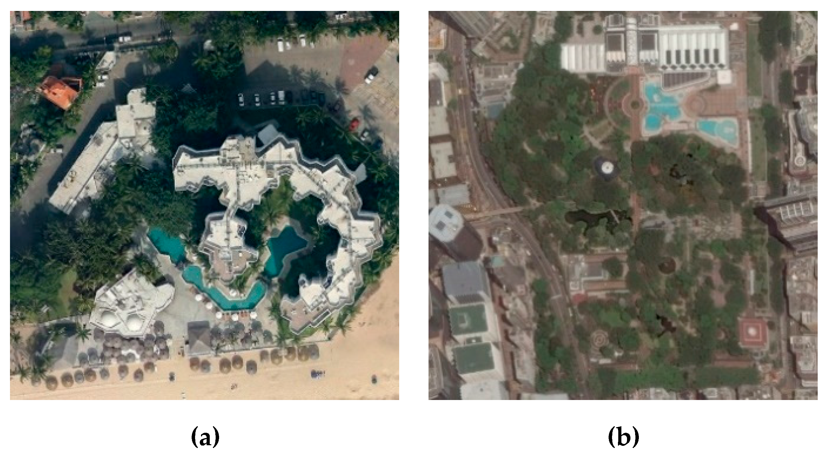
As we can see in Table 2, our ResNet_LGFFE can get 98.62%0.88% in OA, which is superior to most methods and slightly worse than the methods ARCNet [17] and LGFF [33]. The best performance, 99.76%, is acquired by LGFF [33], which is close to 100%. Because ResNet_LGFFE is implemented by combining the ResNet50 with the designed local-global-fusion feature extractor, the comparison between ResNet_LGFFE and Finetune_ResNe50 is necessary to show the effectiveness of LGFFE. The results shown in Table 2 show that ResNet_LGFFE yields a 4% increase in OA compared to Finetune_ResNet50. This confirms that the LGFFE module is efficient and contributes to the better performance of classification accuracy. The CMs of these two methods are shown in Figure 8 (a) and (b). Many categories are fully predicted correctly in Figure 8 (a). But many images in the category 13 (mobile home park) are incorrectly classified as category 12 (medium residential). Based on the samples from these two categories shown in Figure 9, there is some similar local and semantic information between the two images. Unlike the baseline method, our ResNet_LGFFE focuses on the regional feature resulting in this kind of misclassification. Notably, many methods have higher accuracy in the UCM dataset. Overall, these experimental results show that the LGFFE module is helpful to improve the representation ability of feature embedding by fusing the local and global features, although some misclassification may be caused by more attention to regional feature. Further challenging experiments are needed to conduct to verify the effectiveness of LGFFE.
4.3.2. Experiment 2: Aerial Image Dataset (AID)
Experiment 2 is conducted on the more challenging dataset, AID, with a larger data size and more categories. AID is widely adopted to verify the effectiveness of the classifier because it is more difficult and challenging than UCM. The experimental results are shown in Table 3. As we can find, our ResNet_LGFFE can yield the best performance under the training ratio of both 20% and 50%. Specifically, under the training ratio of 20%, ResNet_LGFFE makes an increase of 2% compared to the ARCNet [17] in OA, and when trained under the training ratio of 50%, the best performance in OA is also acquired by our method, with 1.36% higher than the second best method. In addition, the comparison results between ResNet_LGFFE and baseline ResNet50 can further show the effectiveness of our local-global-fusion feature extractor. The results shown in Table 3 reveal that, compared to the baseline method Finetune_ResNet50, there are almost 4.4% and 5.2% improvements yielded under the two training ratios. This is because our LGFFE captures more silent regional and spatial information on the target areas and generates a more discriminative feature representation.
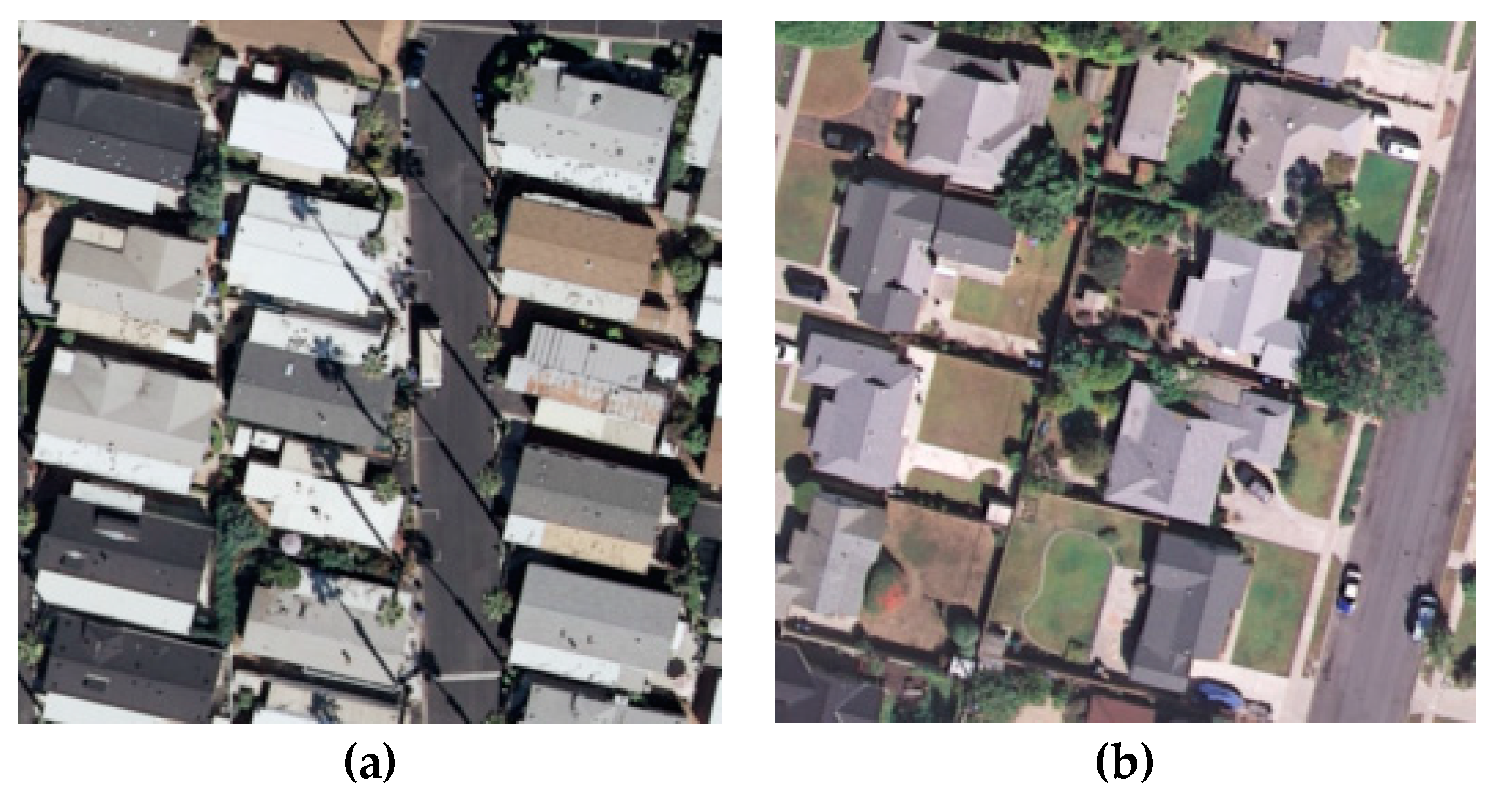
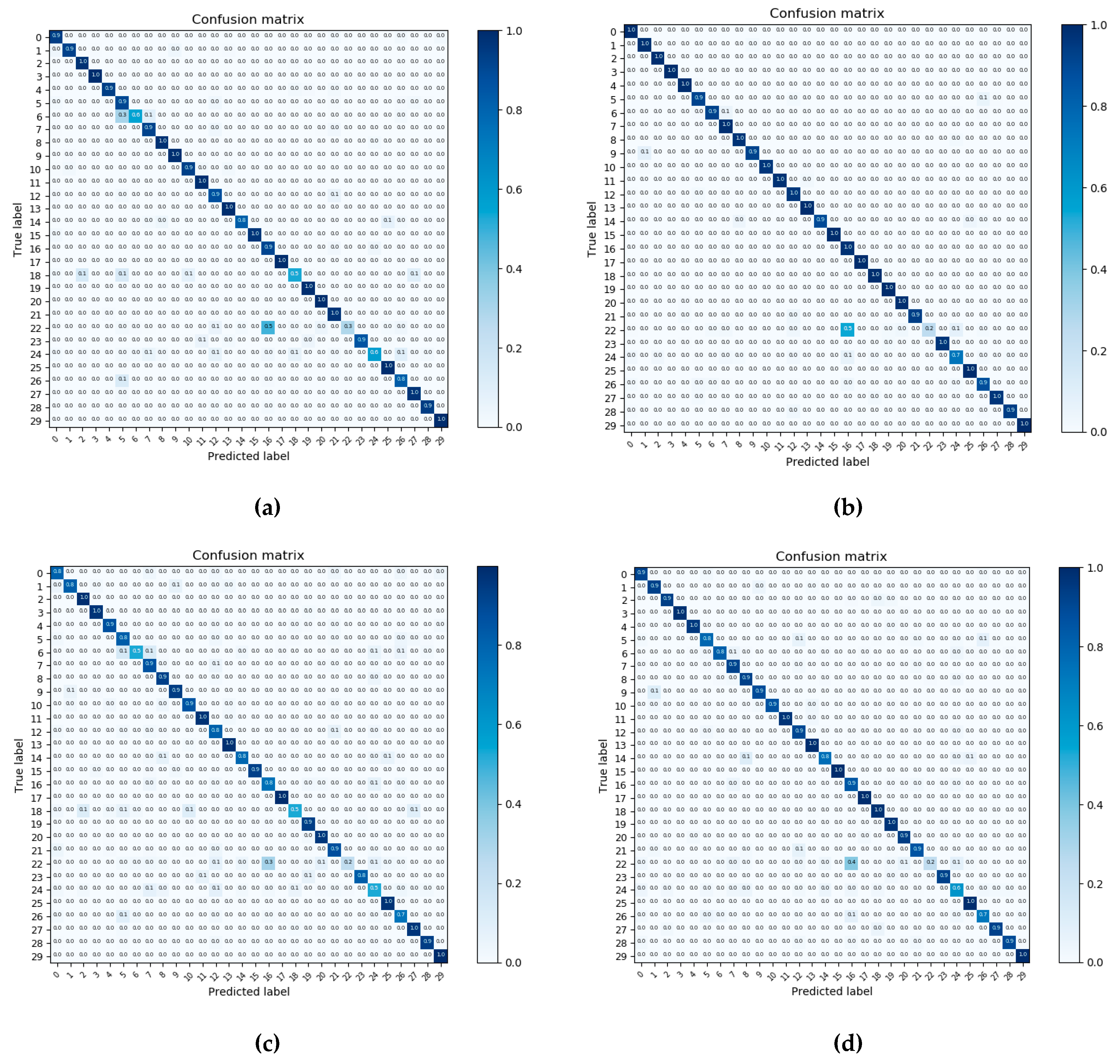
The CMs of ResNet_LGFFE and Finetune_ResNet50 shown in Figure 10 can show our effectiveness more intuitively. The contrasting figure shows that more categories in Figure 10 (a) and (b) are classified correctly, compared to the results in Figure 10 (c) and (d). By comparing Figure 10 (b) and (d), the category 5 (center), 6 (church), 14 (medium residential), 26 (square), and 27 (stadium) have a significantly improved classification accuracy, but category 22 (resort) is incorrectly assigned to category 16 (park). Samples from these two categories are shown in Figure 11. Therefore, under the dataset AID, the LGFFE greatly improves the OA and outperforms the state-of-the-art methods in RSISC. However, it results in slight misclassification as it pays more attention to the regional geometric information.
4.3.3. Experiment 3: NWPU-RESISC45 Dataset (NWPU45)
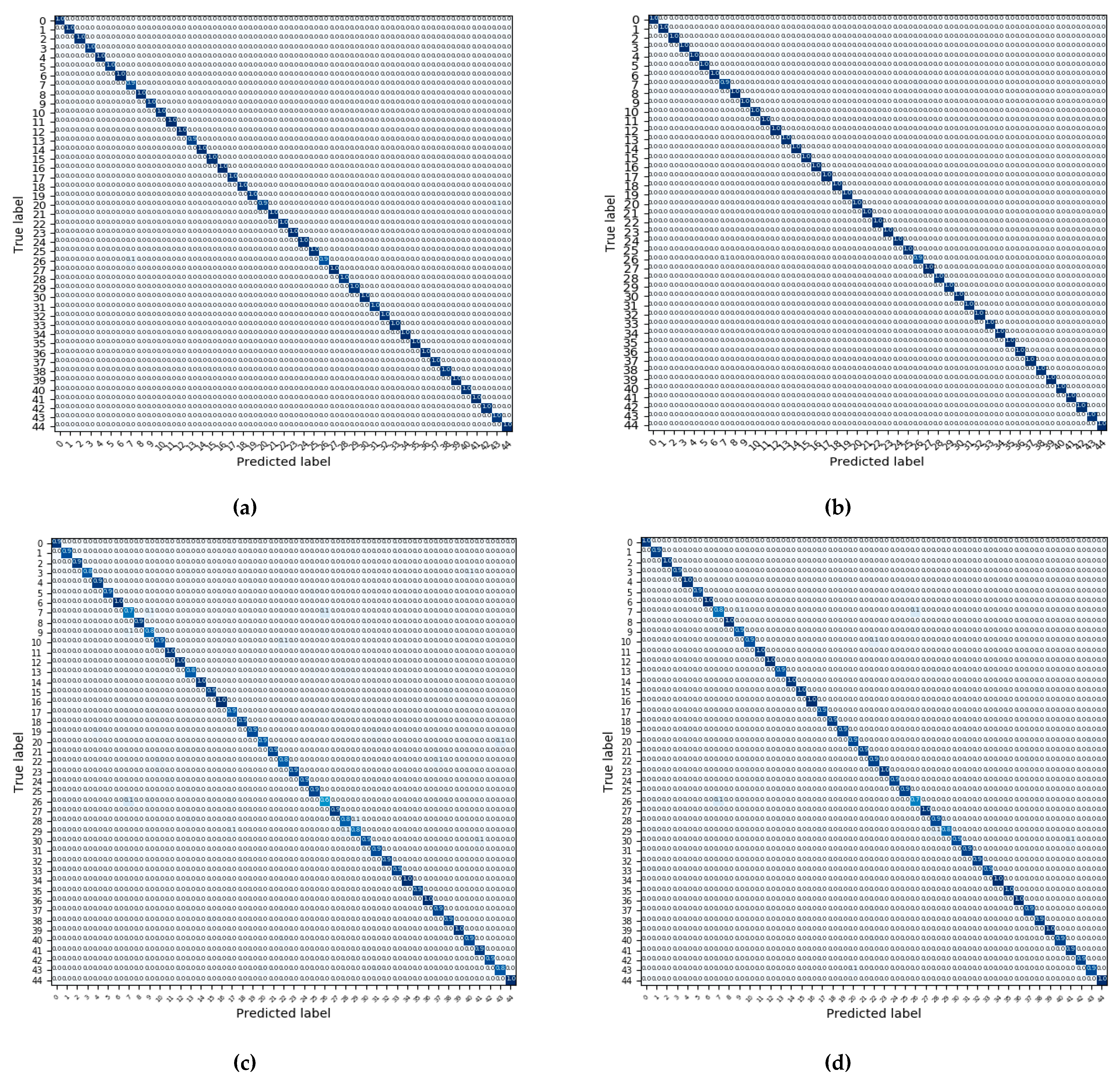
The NWPU45 dataset has the largest amount of data and categories in our experiments. However, the current state-of-the-art methods are not effective enough on the NWPU45 dataset. As we can find in Table 4, our LGFFE is superior to state-of-the-art methods by a large margin. Under the training ratio of 10%, there are improvements of almost 4% and 8% in OA than the methods LGFF [33] and D_CNN [11], respectively. Under the training ratio of 20%, the increases of 2.4% and 7% can be made by our method than the method LGFF [33] and D_CNN [11]. Besides, the same conclusion can be acquired by comparing ResNet_LGFFE with baseline Finetune_ResNet50, that the LGFFE is effective and helpful to boost the discriminative ability of feature representation by capturing the regional geometric features. The CMs of this dataset are shown in Figure 12. Our method achieves nearly 100% classification accuracy in almost all categories except the categories: 7 (church), 13 (freeway), 20 (lake), and 26 (palace), as shown in Figure 12 (a) under the training ratio of 10%, and the categories 7 (church) and 26 (palace), as shown in Figure 12 (b) under the training ratio of 10%. This confirms that the LGFFE can generate a more effective feature representation and improve the performance of scene classification. Compared to the Experiment 1 and 2 on the UCM and AID datasets, in this experiment under the NWPU45 dataset, our method achieves the most significant improvement of classification accuracy, which may be related to the data volume of the dataset. The larger the size of training set, the more full the training of our LGFFE model, and the more distinguishing features can be obtained to have a better feature representation.
4.3.4. Experiment 4: OPTIMAL-31
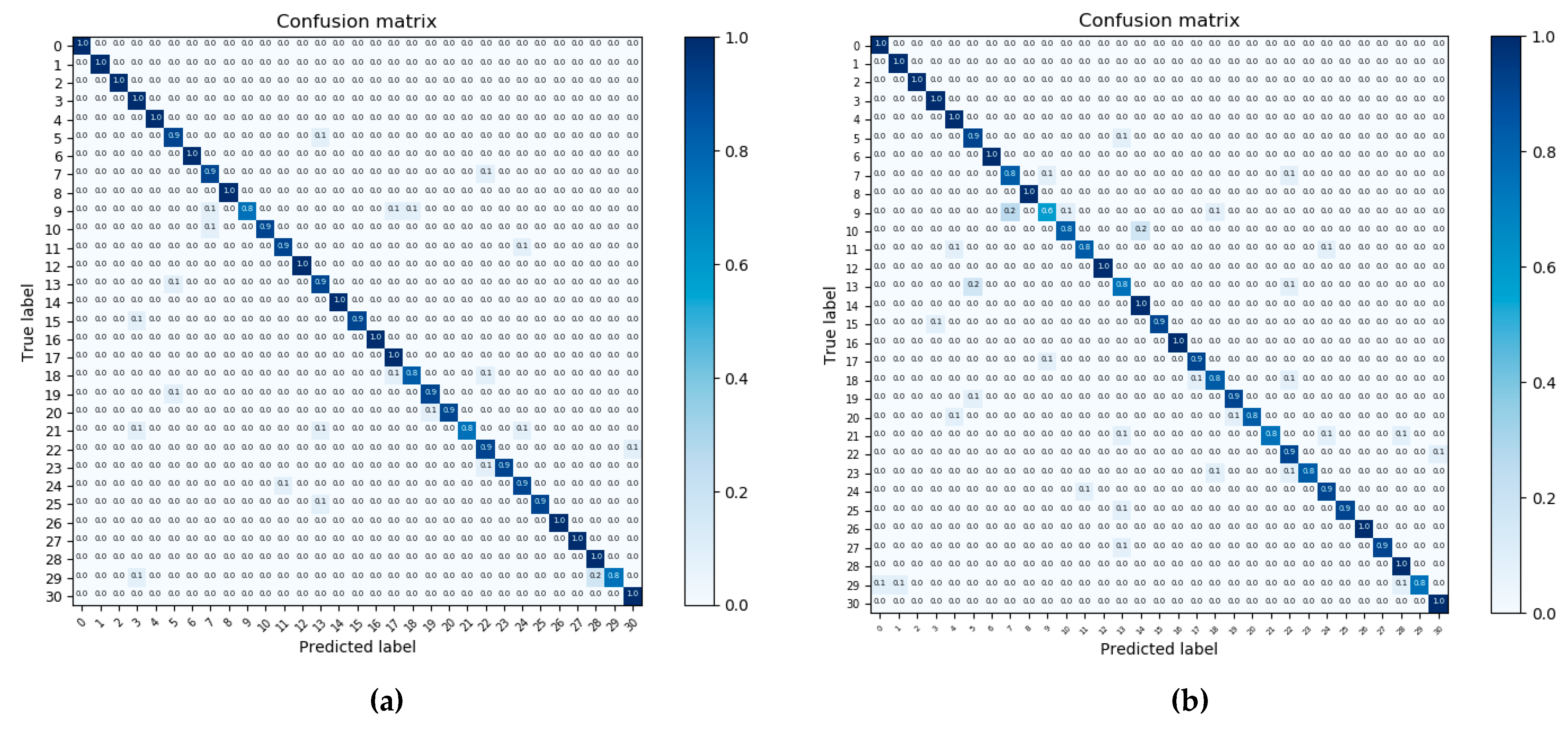
The experiments shown above demonstrate the high performance of the LGFFE. The LGFFE method improves the performance of baseline by a large margin and achieves the state-of-the-art, and the effectiveness and the accuracy of our LGFFE increases when the training set is larger. We further perform experiment 4 on the OPTIMAL-31 dataset to test the performance of the method in small data. As discussed in Section 4.1, this dataset is challenging due to its small data size and many categories. Here, only 48 images from each category are used for training. The experimental results are shown in Table 5. The best performance is 94.55% obtained by our method ResNet_LGFFE, which is 1.85% higher than the original best performance acquired by ARCNet_VGG16 [17]. With the same baseline VGG16, our VGG16_LGFFE has a better performance than the ARCNet_VGG16 [17]. In addition, the comparison results show that our method LGFFE can make an increase of almost 5% and 4% compared to their corresponding baseline VGG16 and ResNet50, and the CMs are shown in Figure 13. Taken together, the designed LGFFE module shows the best performance on a small dataset for the task of scene classification. The effectiveness of our LGFFE on the dataset with less training set can be verified by this experiment.
5. Discussion
The experiments performed in this study show that the proposed LGFFE is effective. The following discussion is given for the experimental results reported here.
5.1. Ablation Studies of our Proposed Local-Global-Fusion Feature Extractor (LGFFE)
To illustrate the effectiveness of our LGFFE and explore the influence of different fusion methods between the local and global features, some ablation studies are conducted in this section. As shown in Table 6, the first two rows in table show the results of baseline and baseline combined with LGFFE. The local feature extractor is very effective in improving the overall accuracy by 4%, 5%, 6%, and 4% on the four datasets. More attention is focused on the silent regions of the image, which is an important supplement to the global features. For the fusion methods, the popular two ways are concatenation and addition to combine the two feature representations. The comparison results of these two methods are provided in the last two rows of Table 6. Overall, the performance of the two methods is close in OA, the concatenation way can have an almost 1% increase compared to the addition way on the four datasets. Besides, the comparison between the baseline method and ResNet_LGFFE_Add can demonstrate the effectiveness of our local feature extraction module. Though the fusion method is not the best, the global feature added by the extracted local feature can outperform the only global feature by a large margin in OA.
5.2. The Limits of the Proposed LGFFE
Based on the analysis provided in Section 3.3, the local feature extraction module proposed in this study is actually a type of global pooling method. Unlike the global average pooling and global max pooling, this new global pooling method leverages on prior knowledge as input to learn the importance of different regional feature representations. It is, therefore, superior to the simple max pooling and average pooling methods. However, the increased performance brings the increased computational costs. With the batch size set to 64 and two NVIDIA GTX 1080Ti GPU used for acceleration, we compare the cost time of one training epoch on the datasets. The results shown in Table 7 display the computation cost between baseline and our LGFFE method on the four datasets. We can find that the computer cost of the proposed LGFFE method is increased by almost 1/3, compared with the baseline. The increased training time is mainly due to the local feature extraction module and the fusion module, which introduce additional components, such as several FC layers and an RNN.
Besides the increase of computer cost, another limitation of the proposed LGFFE is the misclassifications caused by the local feature extractor, as shown in Figure 9 and Figure 11. There may be some similar local regions contained in some scene images, which may be paid more attention by our local feature extraction module and lead to a misclassified result.
6. Conclusions
In this paper, we proposed a novel end-to-end local-global-fusion feature extraction (LGFFE) network for RSISC. The global and local features can be extracted respectively based on the high-level features acquired from the deep CNNs. Specifically, an efficient and simple RNN-based attention module was designed to capture the spatial layout information and context information of different regions. The GRUs were exploited to focus on the key region, suppress the non-critical region, and generate a reweighed regional feature representation by taking a sequence of image patches’ features as input. Finally, the reweighted local feature was fused with the general feature to acquire a more discriminative feature representation for remote sensing images. In the experiments, the proposed method was comprehensively evaluated on four public datasets with different characteristics. The experimental results demonstrate that the proposed method outperforms the existing baseline methods and achieves state-of-the-art results.
Though our proposed LGFFE can achieve better performance, there are still some limits that we cannot neglect. As discussed in Section 5.2, some misclassification may be caused by more attention focused on local regions. In the future, we will explore more effective fusion methods for global features and local features to better integrate the local and global information.
Author Contributions
Conceptualization, Y.L. and W.X.; Formal analysis, Y.C.; Methodology, Y.L. and X.Z.; Software, Y.L. and X.Z.; Supervision, W.X. and Y.C.; Writing—original draft, Y.L.; Writing—review and editing, X.Z., Y.C. and M.C.
Funding
This work was supported by the National Natural Science Foundation of China Grant Nos. 61790550, 61790554 and 91538201. The authors would like to thank the editor andthe anonymous reviewers for their hard work.
Acknowledgments
This work was supported by the National Natural Science Foundation of China (Grant 61790550, 61790554 and 91538201). The authors would like to thank the anonymous reviewers for their hard work.
Conflicts of Interest
The authors declare no conflict of interest.
References
- Cheng, G.; Han, J.; Guo, L.; Liu, Z.; Bu, S.; Ren, J. Effective and Efficient Midlevel Visual Elements-Oriented Land-Use Classification Using VHR Remote Sensing Images. IEEE Trans. Geosci. Remote Sens. 2015, 53, 4238–4249. [Google Scholar] [CrossRef] [Green Version]
- Gómez-Chova, L.; Tuia, D.; Moser, G.; Camps-Valls, G. Multimodal Classification of Remote Sensing Images: A Review and Future Directions. Proc. IEEE. 2015, 103, 1560–1584. [Google Scholar] [CrossRef]
- Cheng, G.; Han, J.; Zhou, P.; Guo, L. Multi-class geospatial object detection and geographic image classification based on collection of part detectors. ISPRS J. Photogramm. Remote Sens. 2014, 98, 119–132. [Google Scholar] [CrossRef]
- Krizhevsky, A.; Sutskever, I.; Hinton, G.E. ImageNet Classification with Deep Convolutional Neural Networks. Adv. Neural Inf. Process. Syst. 2012, 141, 1097–1105. [Google Scholar] [CrossRef]
- Zhang, L.; Zhang, L.; Du, B. Deep Learning for Remote Sensing Data: A Technical Tutorial on the State of the Art. IEEE Geosci. Remote Sens. Mag. 2016, 4, 22–40. [Google Scholar] [CrossRef]
- Cheng, G.; Ma, C.; Zhou, P.; Yao, X.; Han, J. Scene classification of high resolution remote sensing images using convolutional neural networks. In Proceedings of the International Geoscience and Remote Sensing Symposium, Beijing, China, 10–15 July 2016; pp. 767–770. [Google Scholar]
- He, K.; Zhang, X.; Ren, S.; Sun, J. Deep Residual Learning for Image Recognition. In Proceedings of the 2016 IEEE Conference on Computer Vision and Pattern Recognition (CVPR), Las Vegas, NV, USA, 27–30 June 2016; pp. 770–778. [Google Scholar]
- Simonyan, K.; Zisserman, A. Very Deep Convolutional Networks for Large-Scale Image Recognition. In Proceedings of the 2015 International Conference on Learning Representations (ICLR), San Diego, CA, USA, 7–9 May 2015. [Google Scholar]
- Huang, G.; Liu, Z.; Van Der Maaten, L.; Weinberger, K.Q. Densely Connected Convolutional Networks. In Proceedings of the 2017 IEEE Conference on Computer Vision and Pattern Recognition (CVPR), Honolulu, HI, USA, 21–26 July 2017; pp. 2261–2269. [Google Scholar]
- Hu, F.; Xia, G.; Yang, W.; Zhang, L.J. Recent Advances and Opportunities in Scene Classification of Aerial Images with Deep Models. In Proceedings of the 2018 IEEE International Geoscience and Remote Sensing Symposium (IGARSS 2018), Valencia, Spain; 22–27 July 2018; pp. 4371–4374. [Google Scholar]
- Cheng, G.; Yang, C.; Yao, X.; Guo, L.; Han, J. When Deep Learning Meets Metric Learning: Remote Sensing Image Scene Classification via Learning Discriminative CNNs. IEEE Trans. Geosci. Remote Sens. 2018, 56, 2811–2821. [Google Scholar] [CrossRef]
- Liu, Y.; Zhong, Y.; Qin, Q. Scene Classification Based on Multiscale Convolutional Neural Network. IEEE Trans. Geosci. Remote Sens. 2018, 56, 7109–7121. [Google Scholar] [CrossRef] [Green Version]
- Marcos, D.; Volpi, M.; Kellenberger, B.; Tuia, D. Land cover mapping at very high resolution with rotation equivariant CNNs: Towards small yet accurate models. ISPRS J. Photogramm. Remote Sens. 2018, 145, 96–107. [Google Scholar] [CrossRef] [Green Version]
- Cheng, G.; Zhou, P.; Han, J. RIFD-CNN: Rotation-Invariant and Fisher Discriminative Convolutional Neural Networks for Object Detection. In Proceedings of the Computer Vision and Pattern Recognition, Xi’an, China, 26 June–1 July 2016; pp. 2884–2893. [Google Scholar]
- Li, P.; Ren, P.; Zhang, X.; Wang, Q.; Zhu, X.; Wang, L. Region-Wise Deep Feature Representation for Remote Sensing Images. Remote Sens. 2018, 10, 871. [Google Scholar] [CrossRef] [Green Version]
- Yuan, Y.; Fang, J.; Lu, X.; Feng, Y. Remote Sensing Image Scene Classification Using Rearranged Local Features. IEEE Trans. Geosci. Remote Sens. 2019, 57, 1779–1792. [Google Scholar] [CrossRef]
- Wang, Q.; Liu, S.; Chanussot, J.; Li, X. Scene Classification with Recurrent Attention of VHR Remote Sensing Images. IEEE Trans. Geosci. Remote Sens. 2019, 57, 1155–1167. [Google Scholar] [CrossRef]
- Swain, M.J.; Ballard, D.H. Color indexing. Int. J. Comput. Vis. 1991, 7, 11–32. [Google Scholar] [CrossRef]
- Ojala, T.; Pietikainen, M.; Maenpaa, T.J.; Intelligence, M. Multiresolution gray-scale and rotation invariant texture classification with local binary patterns. IEEE Trans. Pattern Anal. Mach. Intell. 2002, 24, 971–987. [Google Scholar] [CrossRef]
- Jain, A.K.; Ratha, N.K.; Lakshmanan, S. Object detection using gabor filters. Pattern Recognit. 1997, 30, 295–309. [Google Scholar] [CrossRef]
- Oliva, A.; Torralba, A. Modeling the Shape of the Scene: A Holistic Representation of the Spatial Envelope. Int. J. Comput. Vis. 2001, 42, 145–175. [Google Scholar] [CrossRef]
- Lowe, D.G. Distinctive Image Features from Scale-Invariant Keypoints. Int. J. Comput. Vis. 2004, 60, 91–110. [Google Scholar] [CrossRef]
- Bay, H.; Tuytelaars, T.; Van Gool, L.J. SURF: Speeded up robust features. Int. J. Comput. Vis. 2006, 3951, 404–417. [Google Scholar]
- Yang, Y.; Newsam, S. Bag-of-visual-words and spatial extensions for land-use classification. In Proceedings of the 18th SIGSPATIAL International Conference on Advances in Geographic Information Systems, San Jose, CA, USA, 2–5 November 2010; pp. 270–279. [Google Scholar]
- Blei, D.M.; Ng, A.Y.; Jordan, M. Latent dirichlet allocation. J. Mach. Learn. Res. 2003, 3, 993–1022. [Google Scholar]
- Zhong, Y.; Cui, M.; Zhu, Q.; Zhang, L. Scene classification based on multifeature probabilistic latent semantic analysis for high spatial resolution remote sensing images. IEEE Trans. Geosci. Remote Sens. 2015, 9, 095064. [Google Scholar] [CrossRef]
- Bosch, A.; Zisserman, A.; Muñoz, X. Scene Classification Via pLSA; Springer: Berlin/Heidelberg, Germany, 2006; pp. 517–530. [Google Scholar]
- Penatti, O.A.B.; Nogueira, K.; Santos, J.A.D. Do deep features generalize from everyday objects to remote sensing and aerial scenes domains? In Proceedings of the 2015 IEEE Conference on Computer Vision and Pattern Recognition Workshops (CVPRW), Boston, MA, USA, 7–12 June 2015; pp. 44–51. [Google Scholar]
- Castelluccio, M.; Poggi, G.; Sansone, C. Verdoliva. Land Use Classification in Remote Sensing Images by Convolutional Neural Networks. arXiv 2015, arXiv:1508.00092. [Google Scholar]
- Nogueira, K.; Penatti, O.A.B.; dos Santos, J.A. Towards better exploiting convolutional neural networks for remote sensing scene classification. Pattern Recognit. 2017, 61, 539–556. [Google Scholar] [CrossRef] [Green Version]
- Zou, Q.; Ni, L.; Zhang, T.; Wang, Q. Deep Learning Based Feature Selection for Remote Sensing Scene Classification. IEEE Geosci. Remote Sens. Lett. 2015, 12, 2321–2325. [Google Scholar] [CrossRef]
- Zhang, F.; Du, B.; Zhang, L. Scene Classification via a Gradient Boosting Random Convolutional Network Framework. IEEE Trans. Geosci. Remote Sens. 2016, 54, 1793–1802. [Google Scholar] [CrossRef]
- Zhu, Q.; Zhong, Y.; Liu, Y.; Zhang, L.; Li, D. A Deep-Local-Global Feature Fusion Framework for High Spatial Resolution Imagery Scene Classification. Remote Sens. 2018, 10, 568. [Google Scholar]
- Lu, X.; Wang, B.; Zheng, X.; Li, X. Exploring Models and Data for Remote Sensing Image Caption Generation. IEEE Trans. Geosci. Remote Sens. 2018, 56, 2183–2195. [Google Scholar] [CrossRef] [Green Version]
- Yang, Z.; He, X.; Gao, J.; Deng, L.; Smola, A. Stacked Attention Networks for Image Question Answering. In Proceedings of the 2016 IEEE Conference on Computer Vision and Pattern Recognition (CVPR), as Vegas, NV, USA, 27–30 June 2016; pp. 21–29. [Google Scholar]
- Gregor, K.; Danihelka, I.; Graves, A.; Rezende, D.J.; Wierstra, D.J. DRAW: A Recurrent Neural Network for Image Generation. In Proceedings of the 32nd International Conference on Machine Learning (ICML), Lille, France, 6–11 July 2015; pp. 1462–1471. [Google Scholar]
- Rush, A.M.; Chopra, S.; Weston, J. A Neural Attention Model for Abstractive Sentence Summarization. arXiv 2015, arXiv:1509.00685. [Google Scholar]
- Hermann, K.M.; Kočiský, T.; Grefenstette, E.; Espeholt, L.; Kay, W.; Suleyman, M.; Blunsom, P. Teaching machines to read and comprehend. In Proceedings of the 28th International Conference on Neural Information Processing Systems-Volume 1, Montreal, QC, Canada, 7–12 December 2015; pp. 1693–1701. [Google Scholar]
- Xiong, W.; Lv, Y.; Cui, Y.; Zhang, X.; Gu, X. A Discriminative Feature Learning Approach for Remote Sensing Image Retrieval. Remote Sens. 2019, 11, 281. [Google Scholar] [CrossRef] [Green Version]
- Chaib, S.; Liu, H.; Gu, Y.; Yao, H. Deep Feature Fusion for VHR Remote Sensing Scene Classification. IEEE Trans. Geosci. Remote Sens. 2017, 55, 4775–4784. [Google Scholar] [CrossRef]
- Xia, G.; Tong, X.; Hu, F.; Zhong, Y.; Datcu, M.; Zhang, L. Exploiting Deep Features for Remote Sensing Image Retrieval: A Systematic Investigation. arXiv 2017, arXiv:1707.07321. [Google Scholar]
- Lin, Y.; Pang, Z.; Wang, D.; Zhuang, Y.; Recognition, P. Task-driven Visual Saliency and Attention-based Visual Question Answering. arxiv 2017, arXiv:1702.06700. [Google Scholar]
- Cho, K.; Van Merrienboer, B.; Gulcehre, C.; Bahdanau, D.; Bougares, F.; Schwenk, H.; Bengio, Y.J. Learning Phrase Representations using RNN Encoder–Decoder for Statistical Machine Translation. In Proceedings of the 2014 IEEE Conference on Computation and Language 2014, Doha, Qatar, 25–29 October 2014; pp. 1724–1734. [Google Scholar]
- Chung, J.; Gulcehre, C.; Cho, K.; Bengio, Y.; Computing, E. Empirical Evaluation of Gated Recurrent Neural Networks on Sequence Modeling. arXiv 2014, arXiv:1412.3555. [Google Scholar]
- Jozefowicz, R.; Zaremba, W.; Sutskever, I. An empirical exploration of recurrent network architectures. In Proceedings of the 32nd International Conference on International Conference on Machine Learning-Volume 37, Lille, France, 6–11 July 2015; pp. 2342–2350. [Google Scholar]
- Xia, G.; Hu, J.; Hu, F.; Shi, B.; Bai, X.; Zhong, Y.; Zhang, L.; Lu, X. AID: A Benchmark Data Set for Performance Evaluation of Aerial Scene Classification. IEEE Trans. Geosci. Remote Sens. 2017, 55, 3965–3981. [Google Scholar] [CrossRef] [Green Version]
- Cheng, G.; Han, J.; Lu, X. Remote Sensing Image Scene Classification: Benchmark and State of the Art. Proc. IEEE 2017, 105, 1865–1883. [Google Scholar] [CrossRef] [Green Version]
Figure 1.
Some example images for remote sensing image scene classification. (a–c) denote the farmland, airport and airport from dataset AID, respectively. (d–f) denote the runway, airplane and airplane from dataset UC Merced, respectively.
Figure 1.
Some example images for remote sensing image scene classification. (a–c) denote the farmland, airport and airport from dataset AID, respectively. (d–f) denote the runway, airplane and airplane from dataset UC Merced, respectively.

Figure 2.
The framework of our proposed discriminative feature learning approach.

Figure 3.
Framework of global feature extraction module.

Figure 4.
Illustration of the motivation for our local feature extraction module, visual geometry group network 16 (VGG16) is taken as an example here.
Figure 4.
Illustration of the motivation for our local feature extraction module, visual geometry group network 16 (VGG16) is taken as an example here.

Figure 5.
The architecture of the gated recurrent units (GRU).

Figure 6.
The architecture of the recurrent neural network (RNN)-based attention module.

Figure 7.
The framework of the local feature extraction module.

Figure 8.
Confusion matrix (CM) on the UCM dataset: (a) The CM of ResNet_LGFFE on the UCM dataset, (b) The CM of Finetune_ResNet50 on the UCM dataset.
Figure 8.
Confusion matrix (CM) on the UCM dataset: (a) The CM of ResNet_LGFFE on the UCM dataset, (b) The CM of Finetune_ResNet50 on the UCM dataset.

Figure 9.
Examples of misclassified data from the UCM dataset: (a) mobile home park, (b) medium residential.
Figure 9.
Examples of misclassified data from the UCM dataset: (a) mobile home park, (b) medium residential.

Figure 10.
CMs on dataset AID: (a) The CM of the ResNet_LGFFE under the training ratio of 20%, (b) The CM of the ResNet_LGFFE under the training ratio of 50%, (c) The CM of the Finetune_ResNet50 under the training ratio of 20%, and (d) The CM of the Finetune_ResNet50 under the training ratio of 50%.

Figure 11.
Misclassified examples from the AID: (a) resort, (b) park.

Figure 12.
The CMs on dataset NWPU45: (a) The CM of ResNet_LGFFE under the training ratio of 10%, (b) The CM of ResNet_LGFFE under the training ratio of 20%, (c) The CM of Finetune_ResNet50 under the training ratio of 10%, and (d) The CM of Finetune_ResNet50 under the training ratio of 20%.
Figure 12.
The CMs on dataset NWPU45: (a) The CM of ResNet_LGFFE under the training ratio of 10%, (b) The CM of ResNet_LGFFE under the training ratio of 20%, (c) The CM of Finetune_ResNet50 under the training ratio of 10%, and (d) The CM of Finetune_ResNet50 under the training ratio of 20%.

Figure 13.
CMs on dataset Optimal-31: (a) CM of method ResNet_LGFFE, (b) CM of method Finetune_ResNet50.
Figure 13.
CMs on dataset Optimal-31: (a) CM of method ResNet_LGFFE, (b) CM of method Finetune_ResNet50.


Table 1.
Performance of different deep CNNs on the Aerial Image dataset (AID).
| Methods | Training Radio | |
|---|---|---|
| 20% | 50% | |
| VGG16_LGFFE | 89.36 | 94.06 |
| VGG19_LGFFE | 89.61 | 93.94 |
| ResNet_LGFFE | 90.83 | 94.46 |
LGFFE denotes the proposed local-global-fusion feature extractor module.
Table 2.
Overall accuracy (OA) (%) of different methods on the UC Merced Land-Use (UCM) dataset under the training ratio of 80%.
Table 2.
Overall accuracy (OA) (%) of different methods on the UC Merced Land-Use (UCM) dataset under the training ratio of 80%.
| Methods | Overall Accuracy (%) |
|---|---|
| VGG16 [46] | 95.211.2 |
| GoogLeNet [46] | 94.310.89 |
| CNN-Region [15] | 95.85 |
| ARCNet [17] | 99.120.4 |
| LGFF [33] | 99.760.06 |
| RL_feature [16] | 94.971.16 |
| Fusion-by-add [40] | 97.421.79 |
| MCNN [12] | 96.660.9 |
| Finetune_ResNet50 | 94.550.96 |
| ResNet_LGFFE (ours) | 98.620.88 |
Table 3.
The OA (%) of different methods on the AID.
| Methods | Training radio | |
|---|---|---|
| 20% | 50% | |
| VGG16 [46] | 86.590.29 | 89.640.30 |
| CaffeNet [46] | 86.860.47 | 89.530.31 |
| GoogLeNet [46] | 83.440.40 | 86.390.55 |
| Fusion-by-add [40] | 91.870.36 | |
| MCNN [12] | 91.800.22 | |
| ARCNet [17] | 88.750.40 | 93.100.55 |
| Finetune_ResNet50 | 86.480.49 | 89.220.34 |
| ResNet_LGFFE (ours) | 90.830.55 | 94.460.48 |
Table 4.
The OA (%) of different methods on the NWPU45 dataset.
| Methods | Training Radio | |
|---|---|---|
| 10% | 20% | |
| AlexNet [47] | 81.220.19 | 85.160.18 |
| VGG_16 [47] | 87.150.45 | 90.360.18 |
| GoogleNet [47] | 86.020.18 | 86.020.18 |
| D_CNN [11] | 89.220.5 | 91.890.22 |
| LGFF [33] | 93.610.1 | 96.370.05 |
| Finetune_ResNet50 | 89.880.26 | 92.350.19 |
| ResNet_LGFFE (ours) | 97.560.08 | 98.790.04 |
Table 5.
The OA (%) of different methods on the OPTIMAL-31 dataset.
| Methods | Overall Accuracy (%) |
|---|---|
| VGG_VD_16 [46] | 89.120.35 |
| Finetune_GoogLeNet [17] | 82.570.12 |
| Finetune_VGG16 [17] | 87.450.45 |
| Finetune_Alexnet [17] | 81.220.19 |
| ARCNet_VGG16 [17] | 92.700.35 |
| ARCNet_Resnet34 [17] | 91.280.45 |
| Finetune_ResNet50 | 90.460.38 |
| VGG16_LGFFE (ours) | 92.910.26 |
| ResNet_LGFFE (ours) | 94.550.36 |
Table 6.
The OA (%) of different methods removing or changing one part of our LGFFE on four public datasets.
Table 6.
The OA (%) of different methods removing or changing one part of our LGFFE on four public datasets.
| Methods | UCM | AID (50%) | NWPU45 (20%) | OPTIMAL-31 |
|---|---|---|---|---|
| ResNet (baseline) | 94.550.96 | 89.220.34 | 92.350.19 | 90.460.38 |
| ResNet_LGFFE _Conc (ours) | 98.620.88 | 94.460.48 | 98.790.04 | 94.550.36 |
| ResNet_LGFFE _Add | 97.230.86 | 93.780.51 | 97.860.09 | 94.170.39 |
Table 7.
Comparison of the computer costs between the proposed LGFFE and baseline among the four public datasets.
Table 7.
Comparison of the computer costs between the proposed LGFFE and baseline among the four public datasets.
| Methods | UCM | AID (50%) | NWPU45 (20%) | OPTIMAL-31 |
|---|---|---|---|---|
| ResNet (baseline) | 9 s | 29 s | 35 s | 8 s |
| ResNet_LGFFE(ours) | 13 s | 39 s | 49 s | 12 s |
© 2019 by the authors. Licensee MDPI, Basel, Switzerland. This article is an open access article distributed under the terms and conditions of the Creative Commons Attribution (CC BY) license (http://creativecommons.org/licenses/by/4.0/).
Share and Cite
MDPI and ACS Style
Lv, Y.; Zhang, X.; Xiong, W.; Cui, Y.; Cai, M. An End-to-End Local-Global-Fusion Feature Extraction Network for Remote Sensing Image Scene Classification. Remote Sens. 2019, 11, 3006. https://0-doi-org.brum.beds.ac.uk/10.3390/rs11243006
AMA Style
Lv Y, Zhang X, Xiong W, Cui Y, Cai M. An End-to-End Local-Global-Fusion Feature Extraction Network for Remote Sensing Image Scene Classification. Remote Sensing. 2019; 11(24):3006. https://0-doi-org.brum.beds.ac.uk/10.3390/rs11243006
Chicago/Turabian StyleLv, Yafei, Xiaohan Zhang, Wei Xiong, Yaqi Cui, and Mi Cai. 2019. "An End-to-End Local-Global-Fusion Feature Extraction Network for Remote Sensing Image Scene Classification" Remote Sensing 11, no. 24: 3006. https://0-doi-org.brum.beds.ac.uk/10.3390/rs11243006
Note that from the first issue of 2016, this journal uses article numbers instead of page numbers. See further details here.