Improvement of Split-Window Algorithm for Land Surface Temperature Retrieval from Sentinel-3A SLSTR Data Over Barren Surfaces Using ASTER GED Product

Abstract

Land surface temperature (LST) is a key variable influencing the energy balance between the land surface and the atmosphere. In this work, a split-window algorithm was used to calculate LST from Sentinel-3A Sea and Land Surface Temperature Radiometer (SLSTR) thermal infrared data. The National Centers for Environmental Prediction (NCEP) reanalysis atmospheric profiles combined with the radiation transport model MODerate resolution atmospheric TRANsmission version 5.2 (MODTRAN 5.2) were utilized to obtain atmospheric water vapor content (WVC). The ASTER Global Emissivity Database Version 3 (ASTER GED v3) product was utilized to estimate surface emissivity in order to improve the accuracy of LST estimation over barren surfaces. Using a simulation database, the coefficients of the algorithm were fitted and the performance of the algorithm was evaluated. The root-mean-square error (RMSE) values of the differences between the estimated LST and the actual LST of the MODTRAN radiative transfer simulation at each WVC subrange of 0–6.5 g/cm² were less than 1.0 K. To validate the retrieval accuracy, ground-based LST measurements were collected at two relatively homogeneous desert study sites in Dalad Banner and Wuhai, Inner Mongolia, China. The bias between the retrieved LST and the in situ LST was about 0.2 K and the RMSE was about 1.3 K at the Dalad Banner site, whereas they were approximately -0.4 and 1.0 K at the Wuhai site. As a reference, the retrieved LST was compared with the operational SLSTR LST product in this study. The bias between the SLSTR LST product and the in situ LST was approximately 1 K and the RMSE was approximately 2 K at the Dalad Banner site, whereas they were approximately 1.1 and 1.4 K at the Wuhai site. The results demonstrate that the split-window algorithm combined with improved emissivity estimation based on the ASTER GED product can distinctly obtain better accuracy of LST over barren surfaces.

1. Introduction

As a crucial parameter in the global energy balance and environmental monitoring [1,2,3,4], land surface temperature (LST) plays an essential role in evapotranspiration estimation [5,6,7,8], hazard monitoring [9], fire detection [10,11], and global climate change studies [12]. Remote sensing is the only possible technique that can obtain high-spatiotemporal LST at localized and worldwide scales [13,14].

In recent decades, various methods and algorithms have been proposed for retrieving LST from thermal infrared (TIR) satellite data, including single-channel (SC) algorithms [15,16,17], split-window (SW) algorithms [18,19,20], a temperature and emissivity separation (TES) algorithm [21], and a physics-based day and night (D/N) algorithm [22]. These algorithms have been used to generate operational LST products, which are listed in

Table 1. Summary of operational LST products retrieved from polar-orbiting satellite TIR data.

Product Name	Retrieval Algorithm	Temporal Resolution	Spatial Resolution	Available Period	Reference
MxD11	SW algorithm	2 times per day	1 km	2000-02-24 to Present	Becker and Li [18]; Wan and Dozier [26]
MxD11B1	D/N algorithm	2 times per day	6 km	2000-02-24 to Present	Wan and Li [22]
MxD21	TES algorithm	2 times per day	1 km	2000-02-24 to Present	Gillespie, et al. [21]; Hulley and Hook [32]
AST_08	TES algorithm	16 days	90 m	2000-03-04 to Present	Gillespie, et al. [21]
VIIRS VNP21	TES algorithm	2 times per day	750 m	2012-01-19 to Present	Gillespie, et al. [21]; Hulley, et al. [33]
VIIRS EDR	SW algorithm	2 times per day	750 m	2012-08-10 to Present	Yu, et al. [34]
AASTR LST	SW algorithm	35 days	1 km	2002-05-20 to 2012-04-08	Prata [35]
SLSTR LST	SW algorithm	27 days	1 km	2018-04-05 to Present	Prata [35]
Landsat LST	SC algorithm	16 days	30 m	2000-08-16 to Present	Malakar, et al. [1]

.

As shown in Table 1, split-window algorithms are among the most widely used algorithms for LST retrieval from TIR data. Among various input parameters of split-window algorithms, surface emissivity is significant and greatly influences the sensitivity of the algorithms [23]. Previous studies have shown that an uncertainty of 0.01 in surface emissivity could lead to an error of approximately 0.5 K in the retrieved LST [24]. A variety of methods have been proposed for estimating surface emissivity, including a classification-based emissivity method (CBEM) and a normalized difference vegetation index (NDVI)-based emissivity method (NBEM) [23,25]. CBEM has been frequently used to estimate surface emissivity in the retrieval of operational LST products, for example, MODIS, VIIRS, and Sea and Land Surface Temperature Radiometer (SLSTR) LST products [26]. Snyder and Wan [27] pointed out that the accuracy of surface emissivity is worse than 0.01 over barren surfaces. Several studies have indicated that the V5 MODIS LST product is significantly underestimated over barren surfaces due to the overestimation of surface emissivity [28,29]. Therefore, it is necessary to increase the estimation accuracy of emissivity over barren surfaces in order to obtain highly accurate LST retrieval from TIR data using a split-window algorithm. There are some existing studies on improving the accuracy of surface emissivity for VIIRS and Landsat 8 satellite data [30,31]. In those studies, the ASTER Global Emissivity Database Version 3 (ASTER GEDv3) product was used to derive soil emissivity combined with fractional vegetation cover and the ASTER spectral library. Inspired by those ideas, we made some modifications and then applied the method to estimate surface emissivity for Sentinel-3A SLSTR data.

The main objective of this study was to retrieve Sentinel-3A SLSTR LST using a split-window algorithm with high-accuracy estimation of surface emissivity based on the ASTER GEDv3 product and to compare the accuracies of the retrieved SLSTR LST and the operational SLSTR LST product over barren surfaces. This paper comprises four sections: Section 2 describes the data and materials used in this study, Section 3 introduces the split-window algorithm and the methods for emissivity and atmospheric correction, Section 4 presents the findings and the analysis of the results, and Section 5 provides the discussion and a brief conclusion.

2. Data

2.1. Sentinel-3A SLSTR Data

Sentinel-3A was launched on 16 February 2016 as an important mission of the Global Monitoring for Environmental Security (GMES) program [36,37]. Sentinel-3A has an orbit altitude of 815 km and a revisit period of 27 days. The SLSTR sensor carried by Sentinel-3A is part of the (A)ATSR instrument series. The SLSTR instrument was designed with two observation angles: nadir and backward-viewing zenith angle of 55°. There are nine channels involved in SLSTR ranging from visible to thermal infrared, including three visible and near-infrared (VNIR) channels, three shortwave infrared (SWIR) channels, and three mid-infrared (MIR)/TIR channels (centered at 0.555, 0.659, 0.865, 1.375, 1.610, 2.25, 3.74, 10.85, and 12.0 μm). The level 1 product provides at-sensor radiances for all visible and short-wave infrared channels at a spatial resolution of 0.5 km and brightness temperatures at the top of atmosphere (TOA) for TIR channels at a spatial resolution of 1 km. These data can be downloaded from the European Satellite Agency (ESA) website (https://scihub.copernicus.eu/dhus/#/home).

The ESA has also publicly released the operational SLSTR LST product (SL_2_LST). An emissivity-dependent split-window algorithm was utilized to produce the SLSTR LST product from brightness temperatures at TOA of SLSTR channels 8 and 9 at nadir. This algorithm adopts different coefficients for day and night conditions over different land cover types depending on Globcover products. The Globcover products are produced by ESA and cover two periods: December 2004 to June 2006 and January–December 2009. The SLSTR LST product has been available at the ESA website since April 2018 (https://scihub.copernicus.eu/dhus/#/home).

2.2. ASTER GED Product

The ASTER GEDv3 dataset was applied to estimate surface emissivities for SLSTR TIR channels. This dataset was generated using ASTER data collected at all clear-sky conditions from 2000 to 2008 [38]. It is divided into 1° × 1° scenes, providing products at spatial resolutions of 100 m and 1 km. The products include the average and standard deviation (STD) of emissivity in five ASTER TIR bands, ASTER Global Digital Elevation Model (ASTER GDEM), water mask, average and STD of NDVI, longitude and latitude, and observation times. The accuracy of the emissivities was validated using nine desert sites in the United States and the results showed that the average error in emissivity of five TIR bands was within 0.015 for all validation sites [39]. Several attempts have been made to obtain accurate surface emissivity based on the ASTER GED product [1,40,41,42].

2.3. In Situ Measurements

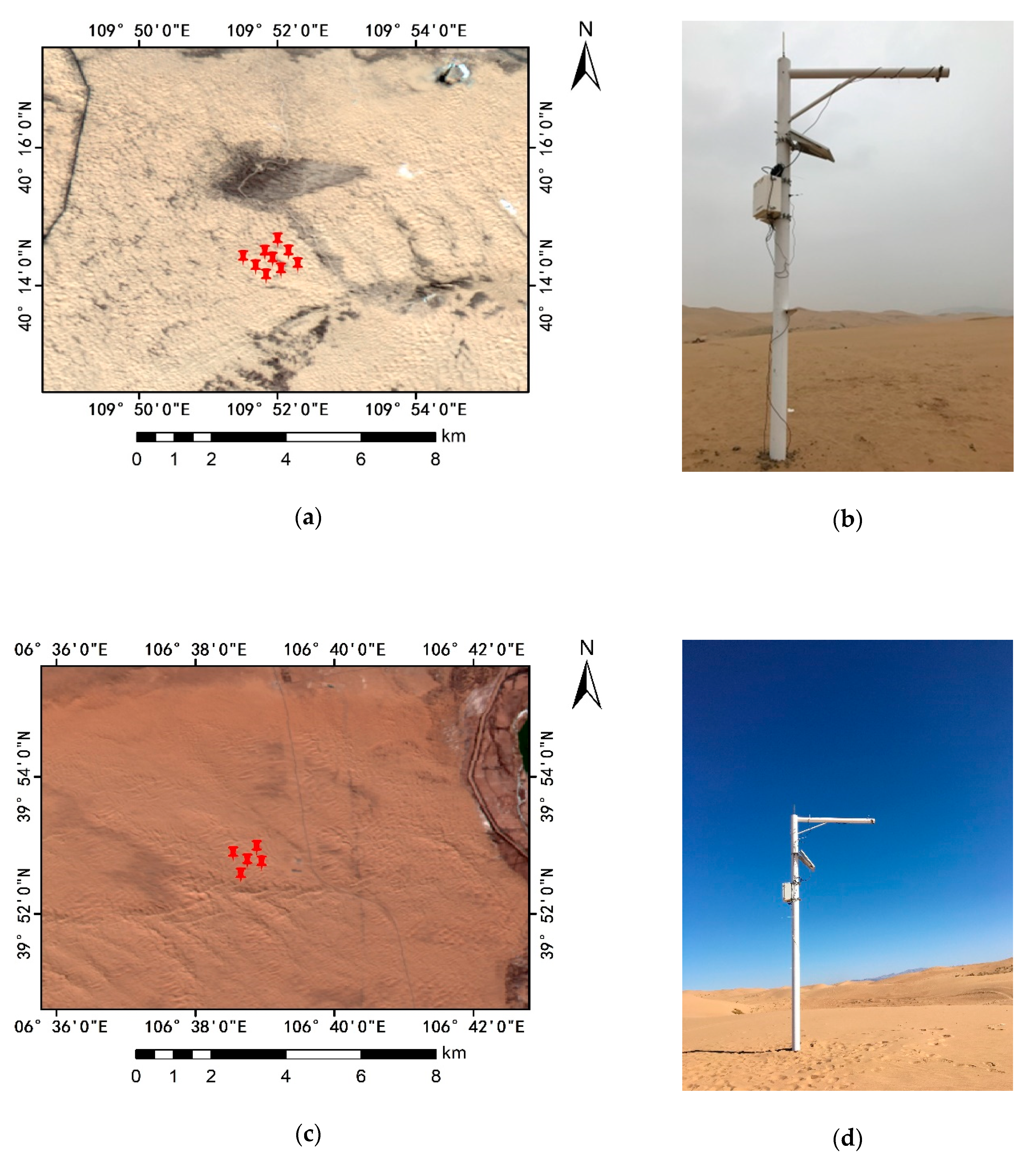
In situ LST measurements collected at two study sites were used for validation of the retrieved SLSTR LST. The two study sites are located in Dalad Banner (109.52°E, 40.14°N) and Wuhai (106.65°E, 39.88°N), Inner Mongolia, China. The land cover type at the two sites is mainly dominated by a relatively homogeneous desert. The two sites have a semiarid temperate continental climate, which has a large amplitude of diurnal temperature variation and less precipitation. Figure 1 shows the geographic location and measurement instrument at the two sites.

To measure ground-based LST, SI-111 thermal infrared radiometers were installed at the two study sites. The radiances were collected by SI-111 thermal infrared radiometers with a spectral range of 8–14 µm. The response time of the SI-111 is 0.6 s and the measurement uncertainty is ±0.2 K. There were nine poles with SI-111 radiometers standing within a 1 km² area at the Dalad Banner site. Ground measurements were collected at an interval of 1 min since July 2018. Five SI-111 radiometers were installed at the Wuhai site and data were collected every 1 min since November 2018. An additional SI-111 at each site was deployed to observe the sky at 53° to measure atmospheric downward radiance. A Nicolet iS50R Fourier transform infrared (FT-IR) spectrometer was used to measure sand samples collected at two sites for the determination of surface emissivity.

In situ LST measurements were calculated using the equation

$$T_s=B^{-1}\left[\frac{L-L_{atm\downarrow }\left(1-\epsilon \right)}{\epsilon }\right]$$

(1)

where T_s is the in situ LST, B is the Planck’s function, ε is the surface emissivity, L is the radiance measured from the surface, and L_atm↓ is the atmospheric downwelling radiance. Planck’s function was used to establish the lookup table between radiance and temperature convolved using the spectral response function of the SI-111 radiometer. Five measurements before and after the acquisition time of SLSTR data for each SI-111 radiometer were averaged to extract in situ LST. An averaged LST of all SI-111 radiometers at each site was used for validation of the retrieved SLSTR LST.

2.4. In Situ LST Uncertainty

Prior to validation of LST using in situ LST measurements, it is important to determine the uncertainty in ground-based LST. The total uncertainty in ground-based LST measurements δ(T_s) is correlative with the uncertainty in radiometer calibration, emissivity estimation, and temporal and spatial variability of LST. It can be expressed as [43]

$$\delta \left(T_S\right)={\left[\delta {\left(\mathrm{cal}\right)}^2+\delta {\left(\mathrm{temp}\right)}^2+\delta {\left(\mathrm{spat}\right)}^2+\delta {\left(\mathrm{emis}\right)}^2\right]}^{\frac{1}{2}}$$

(2)

where δ(cal) is the radiometer calibration error, δ(temp) is the temporal variability of LST at each site, δ(spat) is the spatial thermal variability of each site, and δ(emis) is the uncertainty associated with surface emissivity.

The absolute uncertainty of the SI-111 infrared radiometer is ±0.2 K in the temperature range between 243 and 338 K when the difference between target and sensor temperature is less than 20 K (https://www.apogeeinstruments.com/infraredradiometer/). Before the field experiment, an NPL blackbody was used to calibrate all of the SI-111 radiometers in the laboratory. The absolute accuracy of the blackbody is ±0.1 K at temperatures from 258 to 353 K and the effective emissivity is approximately 0.9998.

In situ LST was averaged in terms of five measurements acquired within 5 min before and after SLSTR acquisition time at each site. To ensure that the uncertainty δ(temp) associated with temporal variability of LST at each site was minimal, the STD of in situ LST measurements was calculated and ensured to be less than 0.2 K.

The uncertainty δ(spat) associated with spatial heterogeneity at each site was analyzed using the 90 m resolution ASTER LST product during the period from July 2018 to March 2019. The STD of 11 × 11 ASTER LST within an SLSTR pixel centered at each site was calculated as an indicator of the spatial thermal variability of each site. The average STD of all available ASTER LST scenes was 1.02 and 0.58 K for Dalad Banner and Wuhai sites, respectively.

The uncertainty in emissivity was approximately 0.01. The error δ(emis) associated with emissivity ranged from 0.3 to 0.5 K. Overall, the total uncertainties in LST measurements were 1.16 and 0.8 K for Dalad Banner and Wuhai sites, respectively.

3. Methodology

3.1. LST Retrieval Algorithm

The split-window algorithm used in this study resembles that of Sobrino and Raissouni [25], which was first proposed for Advanced Very High Resolution Radiometer (AVHRR) scenes. The expression given by Equation (3) was for LST retrieval from Sentinel-3A SLSTR TIR data at nadir,

$$T_S=b_0+b_1{T}_{ch8}+b_2(T_{ch8}-T_{ch9})+b_3{(T_{ch8}-T_{ch9})}^2+(b_4+b_{5}W)(1-\epsilon )+(b_6+b_{7}W)\Delta \epsilon$$

(3)

where T_ch8 and T_ch9 are the TOA brightness temperatures of SLSTR TIR channels 8 and 9, b_k (k = 0–7) are the coefficients of the split-window algorithm, W is the atmospheric water vapor content (WVC) at satellite zenith angle θ (W = W_v/cos(θ)), W_v is the vertical WVC, ε is the average emissivity (ε = (ε_ch8 + ε_ch9)/2), and $\Delta \epsilon$ is the emissivity difference of SLSTR channels 8 and 9 (Δε = ε_ch8 − ε_ch9).

To determine the split-window algorithm coefficients in Equation (3), the radiation transport model MODerate resolution atmospheric TRANsmission version 5.2 (MODTRAN 5.2) and the Thermodynamic Initial Guess Retrieval 2000 (TIGR2000) dataset were used to generate a simulated dataset of TOA brightness temperatures at 11 and 12 μm channels. Sixty cloud-free atmospheric profiles were selected from TIGR2000, which represent global atmospheric and surface situations. The WVC value in the atmosphere ranged from 0 to 6.5 g/cm² and the air temperature (T₀) in the bottom layer of each atmospheric profile varied from 230 to 310 K. For a better simulation of the correlation between T₀ and T_s, the input T_s varied with T₀ for each profile: T_s ranged from T₀ − 5 K to T₀ + 20 K with an interval of 5 K when T₀ was higher than 280 K, whereas T_s ranged from T₀ − 5 K to T₀ + 5 K with an interval of 5 K when T₀ was lower than or equal to 280 K. In the simulations, average emissivity ε was set to vary from 0.9 to 1.0, with an interval of 0.02. 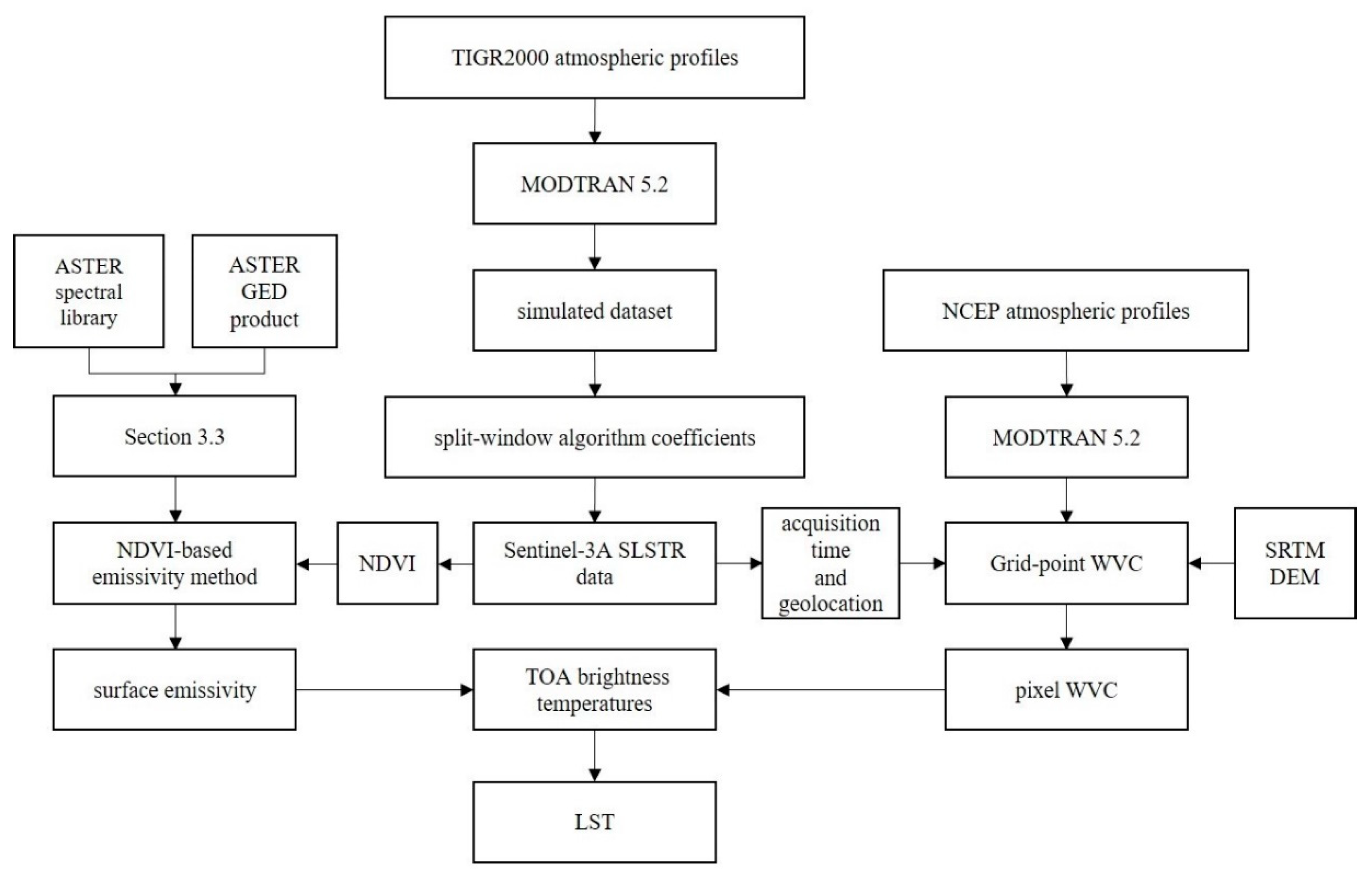Meanwhile, Δε lay in the range from -0.02 to 0.02 with a step of 0.005 [30]. Consequently, the simulation dataset was composed of 30,456 different cases. The flowchart of LST retrieval from Sentinel-3A SLSTR TIR data is shown in Figure 2.

The split-window algorithm coefficients for SLSTR data were determined by least-squares regression analysis in combination with the simulated TOA brightness temperatures of SLSTR TIR channels and the LST input into MODTRAN 5.2. These coefficients are b₀ = -6.49533, b₁ = 1.01933, b₂ = 1.52956, b₃ = 0.247595, b₄ = 69.8631, b₅ = -7.85250, b₆ = -125.574, and b₇ = 16.7550.

3.2. WVC Estimation Method

As shown in Equation (3), atmospheric WVC is a significant input variable in the equation for LST retrieval. In this study, atmospheric WVC was estimated using the National Centers for Environmental Prediction (NCEP) atmospheric profile at the grid resolution of 0.5° × 0.5° provided four times per day (12:00 a.m., 6:00 a.m., 12:00 p.m., and 6:00 p.m. UTC). The NCEP atmospheric profile has been proved to have an accuracy of 0.5 g/cm² for atmospheric WVC [44,45].

To compensate the temporal and spatial discrepancy between SLSTR and the NCEP atmospheric profile and to eliminate error induced by land elevation, interpolation of atmospheric profiles in elevation, space, and time should be conducted to extract atmospheric WVC for each pixel in an SLSTR scene. Considering computational efficiency, five elevation values were preset to perform elevation interpolation with the range of surface elevation corresponding to an SLSTR scene [40]. For each NCEP profile, geographic height, pressure, temperature, and relative humidity were input into MODTRAN 5.2 to calculate atmospheric WVC. In terms of surface elevation obtained from the NASA Shuttle Radar Topographic Mission (SRTM) DEM data at the spatial resolution of 900 m, the atmospheric WVC of each pixel was linearly interpolated at the two closest geographic heights. Because the NCEP profile is available on a fixed grid, the four closest profiles were selected to complete spatial linear interpolation for each pixel. Finally, linear interpolation between two profiles with closest acquisition time of an SLSTR scene was applied to acquire atmospheric WVC for each pixel.

3.3. LSE Estimation Method

Besides atmospheric WVC, surface emissivity is another pivotal variable in the split-window algorithm for LST retrieval. Surface emissivity for a pixel in remote sensing images can be regarded as a weighted combination of vegetation and bare soil emissivities [46] in terms of Equation (4)

$${\epsilon }_i={\epsilon }_{vi}{P}_v+{\epsilon }_{si}(1-P_v)$$

(4)

where i is a channel number, ε_i is the surface emissivity, ε_vi is the channel emissivity of the vegetation component, ε_si is the channel emissivity of the bare soil component, and P_v is the fractional vegetation cover, which can be estimated from NDVI using Equation (5) [47]

$$P_v={\left[\frac{NDVI-NDV{I}_{\min }}{NDV{I}_{\max }-NDV{I}_{\min }}\right]}^2$$

(5)

where NDVI is calculated from surface reflectances in VNIR channels, and NDVI_min and NDVI_max are the NDVI values for full bare soil and full vegetation corresponding to P_v = 0 and P_v = 1, respectively. By the statistics of MODIS NDVI values over 18 years, maximum and minimum of NDVI values were obtained for each pixel in China. The values of NDVI_min and NDVI_max were 0.05 and 0.85, which were extracted from a histogram of NDVI time series. These values are similar to the results in a previous study [48].

Following the work of Wang et al. [30], surface emissivities in SLSTR channels 8 and 9 were estimated by means of the ASTER GED product and fractional vegetation cover. To obtain emissivity information of bare soil background in ASTER channels, Equation (4) can be transformed into the following format

$${\epsilon }_{s\_\mathrm{ASTER}}=\frac{{\epsilon }_{\mathrm{ASTER}}-{\epsilon }_{v\_\mathrm{ASTER}}{P}_{v\_\mathrm{ASTER}}}{1-P_{v\_\mathrm{ASTER}}}$$

(6)

where ε_ASTER is the surface emissivity of a pixel in the ASTER GED product; ε_{s_ASTER} is the emissivity of bare soil in the ASTER pixel; ε_{v_ASTER} is the emissivity of vegetation in the ASTER pixel, which is a mean value of emissivity calculated from several kinds of vegetation in the ASTER spectral library due to the small spectral variation of vegetation in the TIR region; and P_{v_ASTER} is the fractional vegetation cover, which is estimated from ASTER NDVI using Equation (5).

Taking into account the large spectral variation of bare soil in the TIR region, Equation (6) was used to estimate the emissivity of the bare soil component on a pixel-by-pixel basis. Because there are spectral discrepancies between ASTER and SLSTR channels, linear regression formulas were built to convert the emissivity of the bare soil component in ASTER channels to that in SLSTR channels in terms of emissivity spectra in the ASTER spectral library

$${\epsilon }_{s\_\mathrm{SLSTR}8}=0.7{\epsilon }_{s\_\mathrm{ASTER}13}+0.289{\epsilon }_{s\_\mathrm{ASTER}14}+0.01$$

(7)

$${\epsilon }_{s\_\mathrm{SLSTR}9}=-0.277{\epsilon }_{s\_\mathrm{ASTER}13}+0.914{\epsilon }_{s\_\mathrm{ASTER}14}+0.359$$

(8)

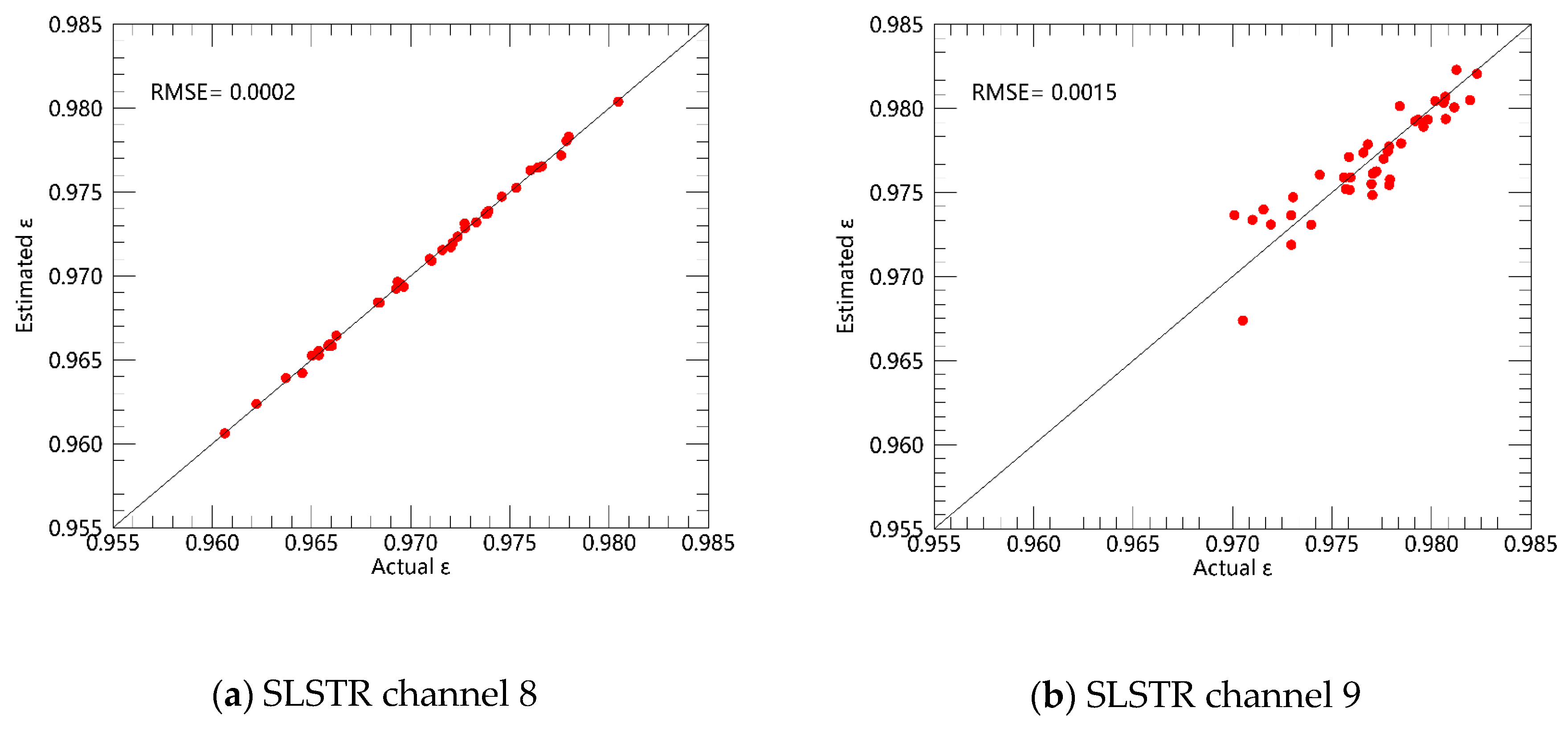
where ε_{s_SLSTR8}, ε_{s_SLSTR9}, ε_{s_ASTER13}, and ε_{s_ASTER14} are the emissivities of bare soil in SLSTR channel 8, SLSTR channel 9, ASTER channel 13, and ASTER channel 14, respectively. The coefficients in Equations (7) and (8) were regressed from the emissivities of bare soil in SLSTR and ASTER TIR channels, which were obtained by convolving emissivity spectra of typical soils in the ASTER spectral library according to the spectral response function in ASTER and SLSTR channels. The scatterplot of the estimated emissivities of bare soil using Equations (7) and (8) and the actual emissivities of bare soil estimated using the ASTER spectral library in SLSTR channels 8 and 9 is shown in Figure 3.

Once the emissivity of bare soil for each SLSTR pixel is available, the surface emissivity for the pixel can be estimated in a manner similar to that of Equation (4)

$${\epsilon }_{\mathrm{SLSTR},i}={\epsilon }_{v\_\mathrm{SLSTR},i}{P}_{v\_\mathrm{SLSTR}}+{\epsilon }_{s\_\mathrm{SLSTR},i}(1-P_{v\_\mathrm{SLSTR}})$$

(9)

where ε_{v_SLSTR,i} is the channel emissivity of the vegetation component, ε_{s_SLSTR,i} is the channel emissivity of the bare soil component, and P_{v_SLSTR} is the fractional vegetation cover calculated by the NDVI value corresponding to Sentinel-3A satellite overpassing time. Because it is difficult to obtain soil moisture information, the emissivity change caused by the impact of soil moisture was not taken into consideration in this study. 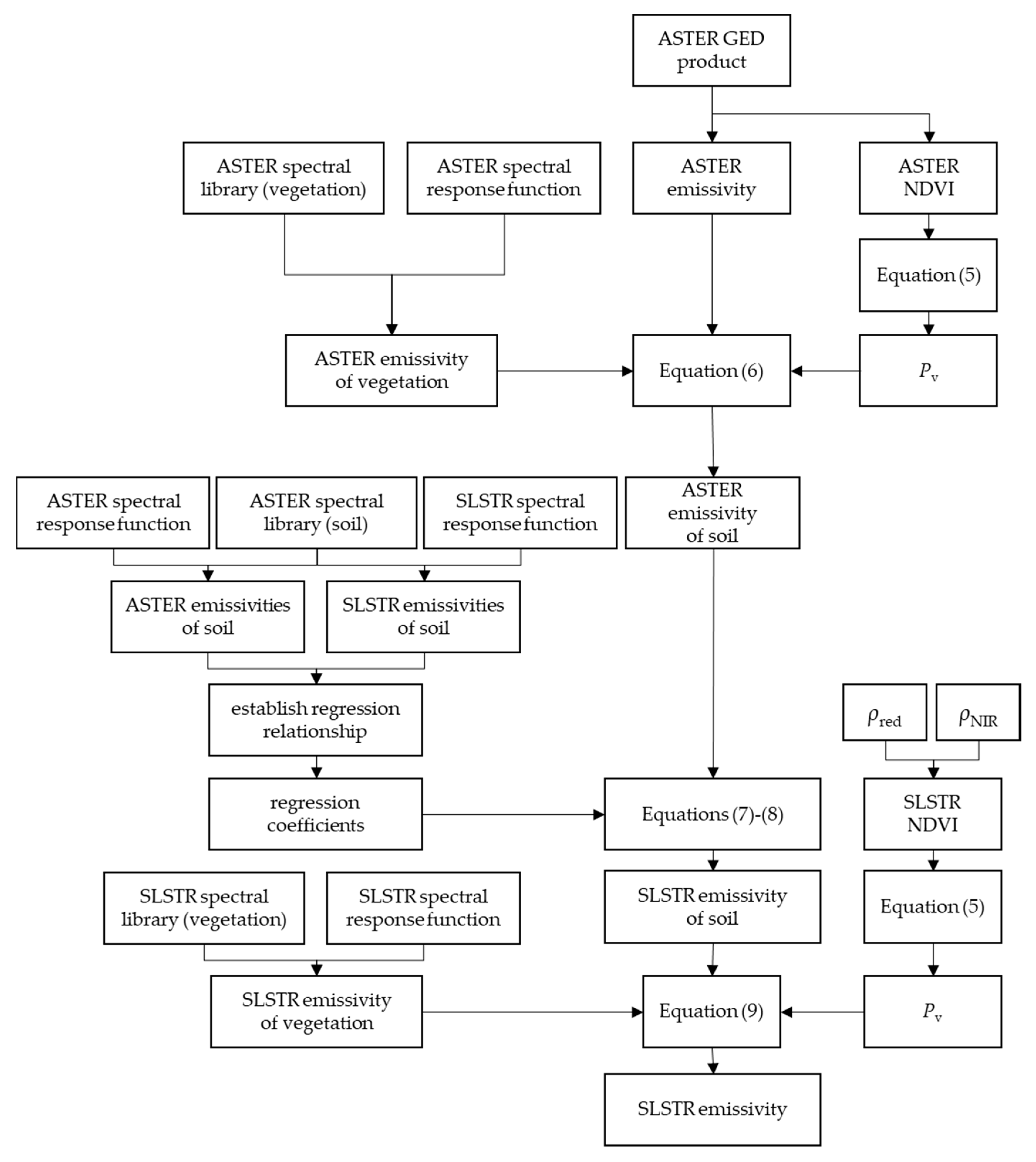Figure 4 shows the flowchart of the estimation of surface emissivity in SLSTR TIR channels from the ASTER GED product.

4. Results

4.1. Accuracy Assessment of Split-Window Algorithm

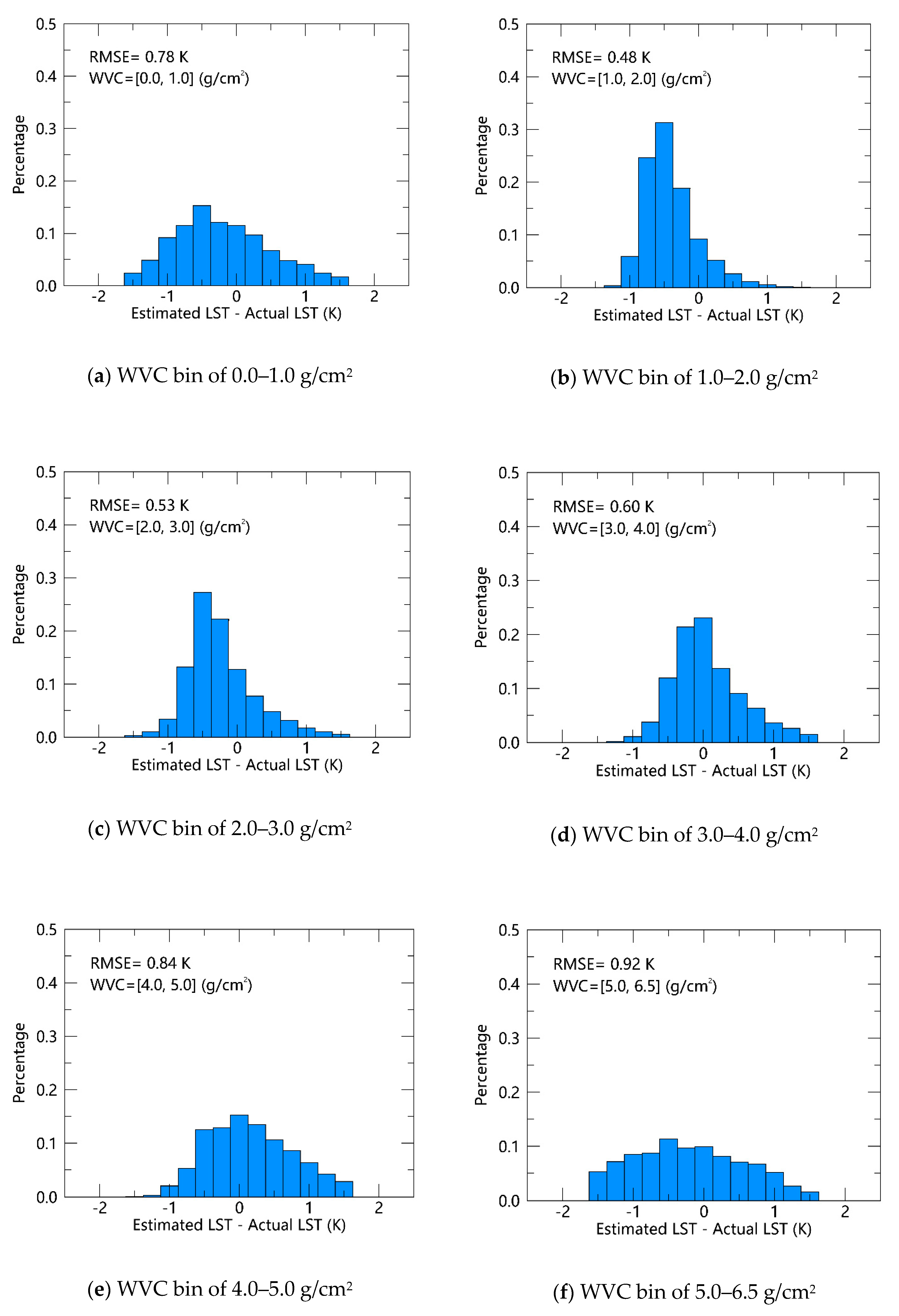
To assess the performance of this split-window algorithm, the differences between the retrieved LST using Equation (3) and the actual LST prescribed in the MODTRAN radiative transfer simulation were divided into six subranges in terms of atmospheric WVC with an increment of 1 g/cm²: 0.0–1.0, 1.0–2.0, 2.0–3.0, 3.0–4.0, 4.0–5.0, and 5.0–6.5 g/cm². Figure 5 shows the histograms of the differences between the estimated and actual LST in each WVC subrange. Most of the differences between the retrieved and actual LST were within ±1 K. The root-mean-square error (RMSE) value was under 1 K for all WVC subranges, and it increased with the increase of the WVC value. The results illustrate that the accuracy of the proposed split-window algorithm was relatively worse under high WVC conditions.

4.2. Comparison of Retrieved LST and SLSTR LST Product

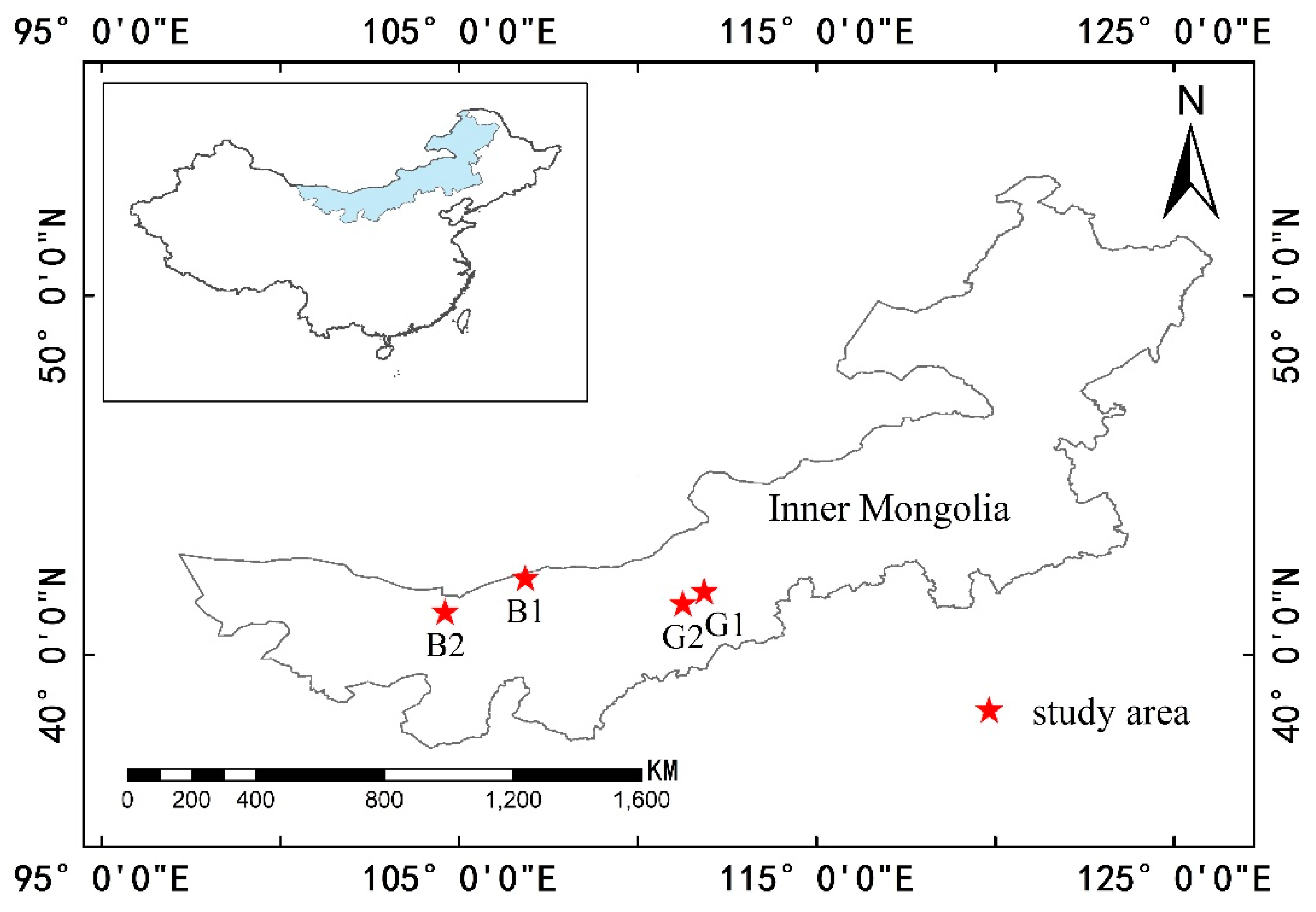
To perform the comparison of the retrieved LST and SLSTR LST product, four study areas of relatively homogeneous land cover type were chosen. According to the classification scheme of the International Geosphere-Biosphere Programme (IGBP), two study areas were identified as grassland (G1 and G2), whereas the other two study areas were classified as bare soil surfaces (B1 and B2). The center geolocation of the four areas is listed in

Table 2. Center geolocation of four selected study areas.

Study Area	Latitude	Longitude	Land Cover Type
G1	41°46′38″	111°52′23″	Grassland
G2	41°26′15″	111°15′59″	Grassland
B1	41°12′22″	104°35′56″	Bare soil
B2	42°8′42″	106°52′8″	Bare soil

and shown in Figure 6.

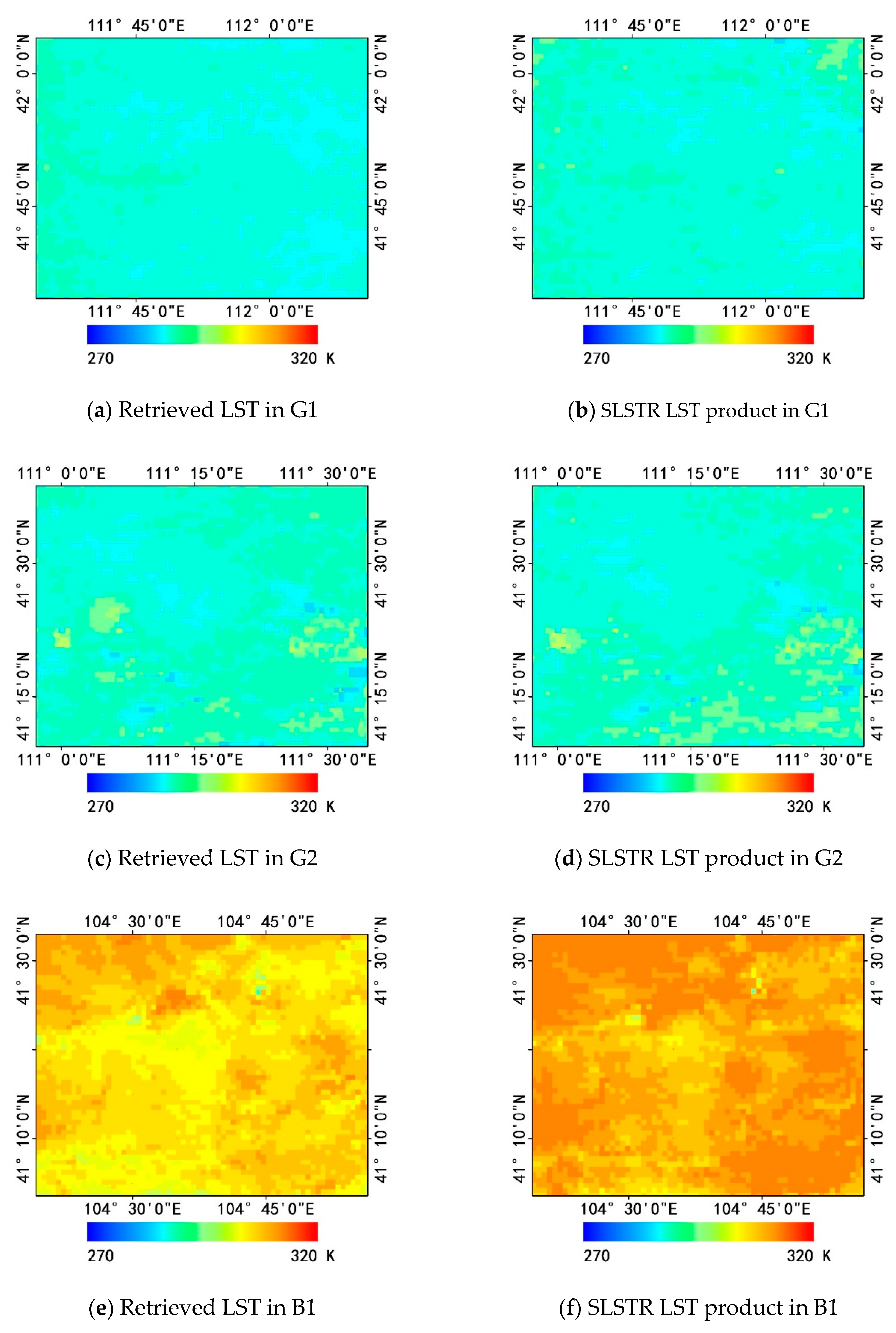
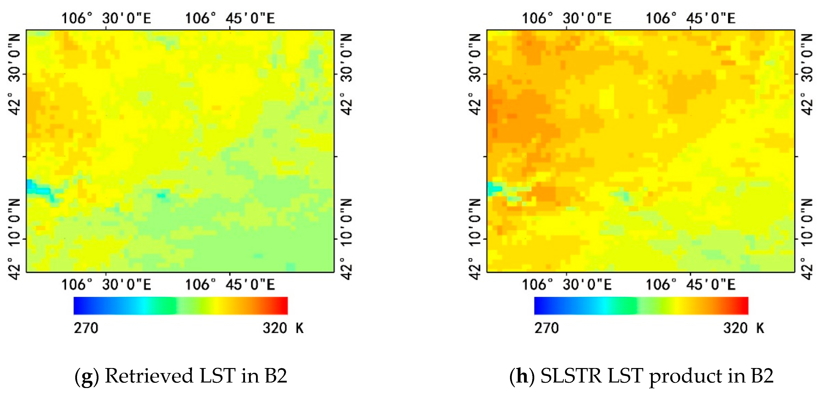
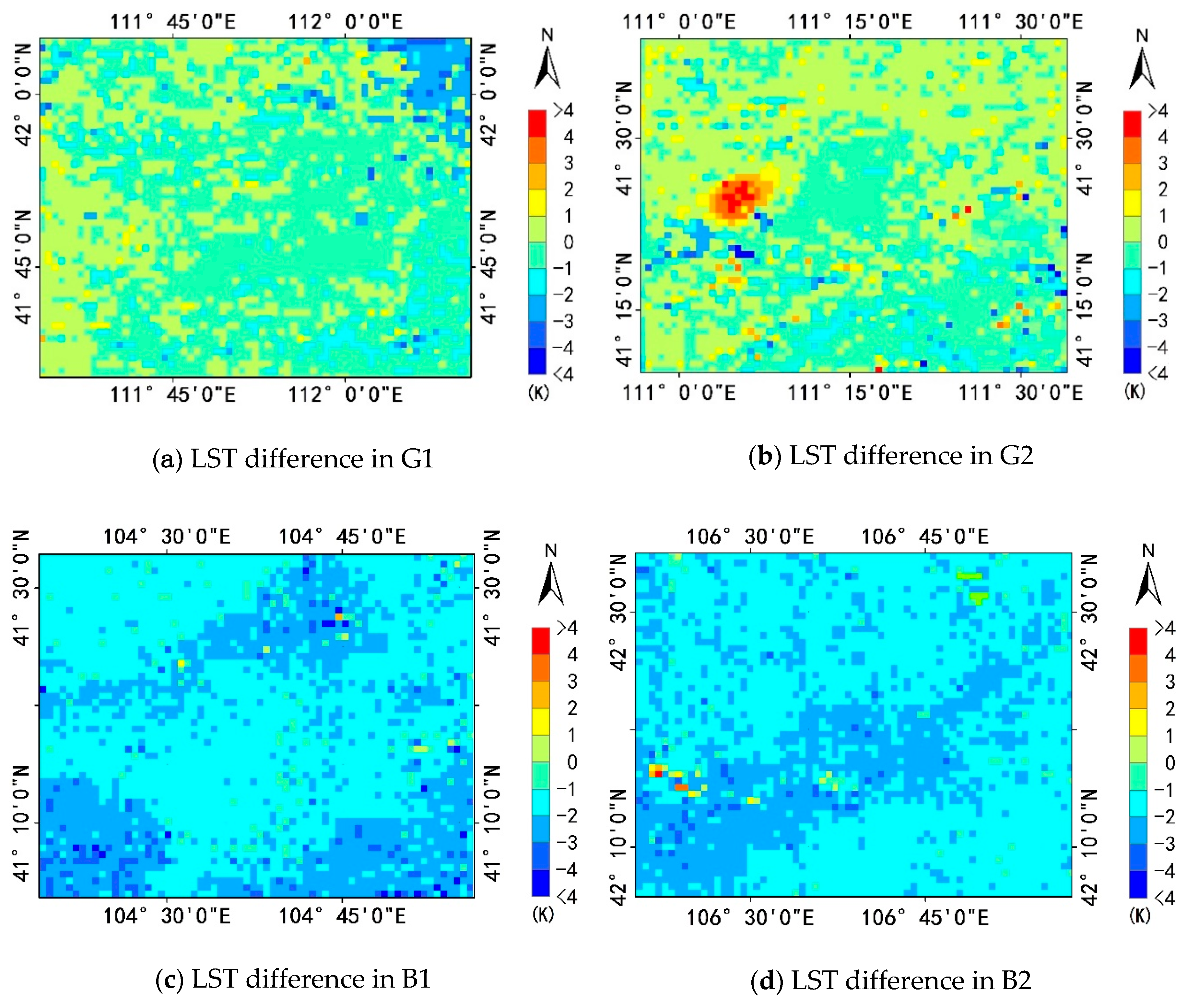
Five clear-sky SLSTR scenes on 14 August 2018, 7 October 2018, 11 October 2018, 22 October 2018, and 14 April 2019 were selected for each study area. The spatial distribution of the retrieved LST and SLSTR LST product over grassland and bare soil surfaces on 7 October 2018 is shown in Figure 7. The differences of retrieved LST and SLSTR LST product were calculated for each study area and are shown in Figure 8. It is obvious that the spatial distribution of the retrieved LST and the SLSTR LST product over grassland surfaces appeared more homogeneous than that over bare soil surfaces. Furthermore, the discrepancy between the retrieved LST and SLSTR LST product over bare soil surfaces was larger than that over grassland surfaces.

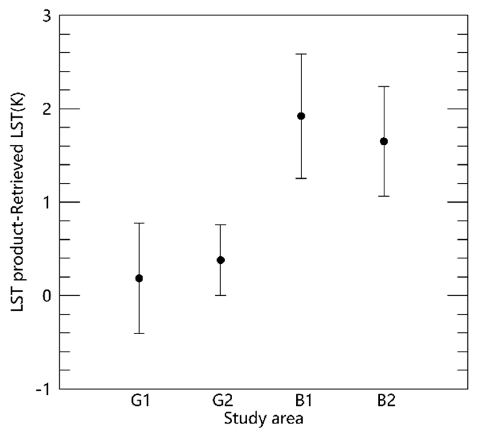
In order to compare the discrepancy between the retrieved LST and SLSTR LST product further, we selected a window of 5 × 5 pixels centered at the geolocation shown in Table 2. For each study area, there were a total of 125 pixels (i.e., 5 × 5 pixels in five SLSTR scenes). Figure 9 shows the statistics for each study area. The biases (RMSE) between the retrieved LST and the SLSTR LST product over two grassland areas were 0.18 K (1.19 K) and 0.38 K (0.85 K), respectively, whereas those over the two bare soil areas were 1.92 K (2.33 K) and 1.65 K (2.03 K), respectively. Both the bias and RMSE over bare soil surfaces were larger than those over grassland surfaces. The results indicate that there was a large discrepancy between the retrieved LST and the SLSTR LST product over barren surfaces.

4.3. LST Validation Using In Situ Measurements

For the validation of retrieved LST, separate collections of in situ measurements at Dalad Banner and Wuhai sites were utilized to assess the accuracy of the retrieved LST. The LST used in the validation process was obtained from the closest pixel to the study sites and guaranteed to be clear-sky measurements using synchronic cloud mask data in the Sentinel-3A SLSTR level 1 product. A pixel was identified as a clear-sky pixel only when its neighboring 5 × 5 pixels were clear-sky pixels. For the two sites, the WVC values obtained from the NCEP reanalysis profiles were quite stable and lay in the range between 0.1 and 1.0 g/cm². 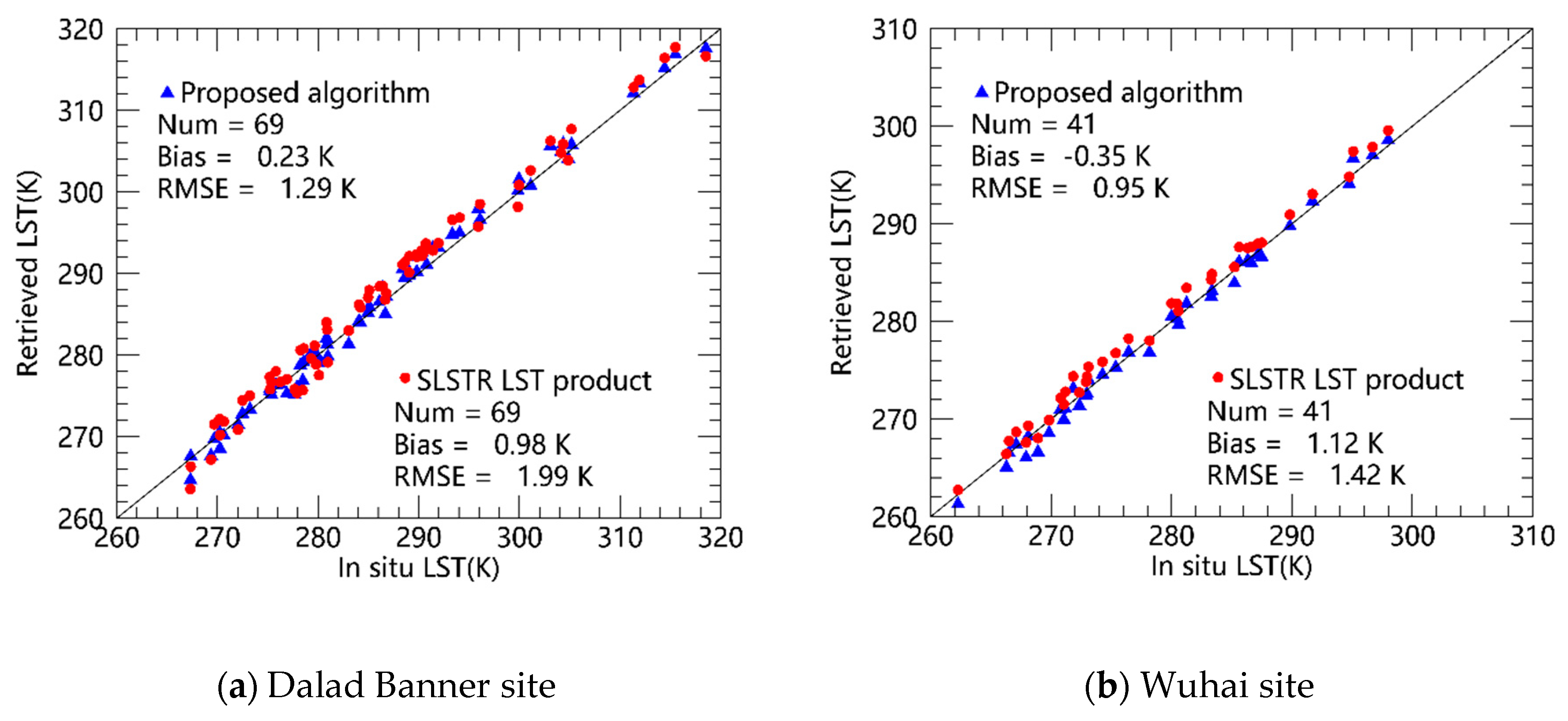Figure 10 provides the results for the retrieved LST. For comparison, the results for the SLSTR LST product are also displayed in Figure 10.

For the Dalad Banner site, there were 69 clear-sky scenes available from July 2018 to April 2019. Compared with the ground-based LST measurements, the bias and RMSE were 0.23 and 1.29 K for the retrieved LST, whereas they were 0.98 and 1.99 K for the SLSTR LST product. The results show that the retrieved LST was closer to the in situ LST measurements than the SLSTR LST product at the Dalad Banner site.

There were 41 clear-sky scenes available during the period between November 2018 and March 2019 at the Wuhai site. The bias between the retrieved LST and the in situ LST was -0.35 K and the RMSE was 0.95 K, whereas those of the differences between the SLSTR LST product and the in situ LST were 1.12 and 1.42 K, respectively.

5. Discussion

The result in the simulated database demonstrates an elevating error along with the increase of the WVC, which is in accordance with previous practice. Though there was a relatively high error in the high WVC subrange, the RMSE lay between ±1 K for all WVC subranges. In addition, the study sites were located in arid and semiarid areas. The WVC values were quite stable and distributed mainly in the range between 0.1 and 1.0 g/cm², in which the accuracy of retrieved LST was relatively high.

It can be derived from Figure 8 that the discrepancy of retrieved LST and the SLSTR LST product over grassland areas was lower than that over bare soil areas. This demonstrates that the emissivity of vegetation is more invariable than that of bare soil. For bare soil surfaces, the spectra of bare soil varies greatly in thermal infrared ranges. The emissivity of different kinds of soil also varies. Therefore, the spatial variety of soil emissivity is naturally higher than that in grassland surfaces. The surface emissivity of bare soil cannot be estimated directly from the ASTER spectral library.

The classification used by the SLSTR LST product was checked and it was found that the pixel was always classified as ‘bare area’ for the Wuhai site. This indicates that the higher error of the SLSTR LST product was mainly induced by the error of soil emissivity. For the Dalad Banner site, the pixel was occasionally misclassified as ‘mosaic vegetation’. The accuracy of the SLSTR LST product was influenced by both the emissivity error and the misclassification. This was also implied by the higher RMSE (1.99 K) of the SLSTR LST product over the Dalad Banner site compared with that (1.42 K) over the Wuhai site (Figure 10).

Ground-based emissivity was estimated by measuring the spectra of the soil samples collected from the study site with a spectrograph and convolving it with the spectral response function of SLSTR TIR channels. For the Dalad Banner site, the emissivity of the soil sample was 0.941 and 0.961 for SLSTR channels 8 and 9, respectively. Correspondingly, the derived emissivity in this study was 0.950 and 0.969 for the two channels. For the Wuhai site, the emissivity of the soil sample was 0.944 and 0.964 for SLSTR channels 8 and 9, respectively, while the derived emissivity was 0.950 and 0.970, respectively. The emissivity that the SLSTR LST product adopts cannot be assessed directly since it is not provided publicly. However, the higher accuracy of the retrieved LST implies that the estimated emissivity performs better compared with the emissivity used by the SLSTR LST product in LST retrieval.

Radiometers only attain measurements from a small area, which can be considered as a point. In contrast, satellites observe the land surface as a plane. Therefore, it is necessary to ensure that the in situ measurements are capable of representing the surface variety in the pixel range in order to convert point measurements to plane measurements. To achieve this, multiple infrared radiometers (nine for the Dalad Banner site and five for the Wuhai site) were distributed across an area of approximately 1 km². The uncertainty associated with the spatial heterogeneity at each site was also calculated in Section 2.4 in order to make the in situ measurement more comparable to satellite observations.

6. Conclusions

In this study, a split-window algorithm was presented to obtain LST from Sentinel-3A SLSTR TIR data. In this algorithm, the atmospheric water vapor content obtained from the NCEP reanalysis profiles was used to compensate atmospheric effects. Surface emissivity was estimated by means of the ASTER GEDv3 product and fractional vegetation cover.

The retrieved LST was compared with the operational SLSTR LST product over four study areas, including two grassland and two barren areas. The discrepancy between the retrieved LST and SLSTR LST product was significant over barren areas, whereas there were similar accuracies for the retrieved LST and SLSTR LST product over grassland areas.

In situ measurements collected at the Dalad Banner and Wuhai sites over a relatively homogeneous desert were utilized to assess the accuracy of the retrieved LST. The retrieved LST exhibited high constancy with in situ LST, with an RMSE of 1.29 K for the Dalad Banner site and 0.95 K for the Wuhai site. In contrast, the numbers between the SLSTR LST product and the in situ LST were 1.99 and 1.42 K for the two study sites.

Compared with the SLSTR LST product, the retrieved LST had better accuracy in terms of bias and RMSE over both of the study sites when validated with in situ LST measurements. The main reason for the lower accuracy of the SLSTR LST product is due to the relatively larger uncertainty in surface emissivity estimation over barren surfaces using the classification-based method. The results indicate that the ASTER GED product has great potential for improving the estimation accuracy of surface emissivity, which could lead to better accuracy of LST retrieval over barren surfaces.

In future work, attempts will be made to develop an algorithm that is more applicable to Sentinel-3A SLSTR data, instead of using an existing algorithm to retrieve LST. We also expect to extend the validation to more study sites over other land cover types, considering that the current validation was restricted to limited sites due to the representativeness of in situ measurements.

References

- Malakar, N.K.; Hulley, G.C.; Hook, S.J.; Laraby, K.; Cook, M.; Schott, J.R. An operational land surface temperature product for Landsat thermal data: Methodology and validation. IEEE Trans. Geosci. Remote Sens. 2018, 56, 5717–5735. [Google Scholar] [CrossRef]
- Song, L.; Kustas, W.P.; Liu, S.; Colaizzi, P.D.; Nieto, H.; Xu, Z.; Ma, Y.; Li, M.; Xu, T.; Agam, N.; et al. Applications of a thermal-based two-source energy balance model using Priestley-Taylor approach for surface temperature partitioning under advective conditions. J. Hydrol. 2016, 540, 574–587. [Google Scholar] [CrossRef] [Green Version]
- Duan, S.B.; Li, Z.L.; Tang, B.H.; Wu, H.; Tang, R. Generation of a time-consistent land surface temperature product from MODIS data. Remote Sens. Environ. 2014, 140, 339–349. [Google Scholar] [CrossRef]
- Zhao, W.; Li, A.; Jin, H.; Zhang, Z.; Bian, J.; Yin, G. Performance evaluation of the triangle-based empirical soil moisture relationship models based on Landsat-5 TM data and in situ measurements. IEEE Trans. Geosci. Remote Sens. 2017, 55, 2632–2645. [Google Scholar] [CrossRef]
- He, M.; Kimball, J.S.; Yi, Y.; Running, S.W.; Guan, K.; Moreno, A.; Wu, X.; Maneta, M. Satellite data-driven modeling of field scale evapotranspiration in croplands using the MOD16 algorithm framework. Remote Sens. Environ. 2019, 230, 111201. [Google Scholar] [CrossRef]
- Song, L.; Liu, S.; Kustas, W.P.; Nieto, H.; Sun, L.; Xu, Z.; Skaggs, T.H.; Yang, Y.; Ma, M.; Xu, T.; et al. Monitoring and validating spatially and temporally continuous daily evaporation and transpiration at river basin scale. Remote Sens. Environ. 2018, 219, 72–88. [Google Scholar] [CrossRef]
- Leng, P.; Song, X.; Duan, S.B.; Li, Z.L. A practical algorithm for estimating surface soil moisture using combined optical and thermal infrared data. Int. J. Appl. Earth Obs. 2016, 52, 338–348. [Google Scholar] [CrossRef]
- Zhao, W.; Li, A.; Deng, W. Surface energy fluxes estimation over the South Asia subcontinent through assimilating MODIS/TERRA satellite data with in situ observations and GLDAS product by SEBS model. IEEE J. STARS 2014, 7, 3704–3712. [Google Scholar] [CrossRef]
- Zhang, Y.; Meng, Q. A statistical analysis of TIR anomalies extracted by RSTs in relation to an earthquake in the Sichuan area using MODIS LST data. Nat. Hazards Earth Syst. Sci. 2019, 19, 535–549. [Google Scholar] [CrossRef] [Green Version]
- Calle, A.; Salvador, P. The active fire FRP estimation: Study on Sentinel-3/SLSTR. IEEE Geosci. Remote Sens. Lett. 2013, 10, 1046–1049. [Google Scholar] [CrossRef]
- He, L.; Li, Z. Enhancement of a fire-detection algorithm by eliminating solar contamination effects and atmospheric path radiance: Application to MODIS data. Int. J. Remote Sens. 2011, 32, 6273–6293. [Google Scholar] [CrossRef]
- Shafia, A.; Nimish, G.; Bharath, H.A. Dynamics of Land Surface Temperature with Changing Land-Use: Building a Climate ResilientSmart City. In Proceedings of the 2018 3rd International Conference for Convergence in Technology (I2CT), Pune, India, 6–8 April 2018; pp. 1–5. [Google Scholar]
- Duan, S.B.; Li, Z.L.; Leng, P. A framework for the retrieval of all-weather land surface temperature at a high spatial resolution from polar-orbiting thermal infrared and passive microwave data. Remote Sens. Environ. 2017, 195, 107–117. [Google Scholar] [CrossRef]
- Li, Z.L.; Tang, B.H.; Wu, H.; Ren, H.; Yan, G.; Wan, Z.; Trigo, I.F.; Sobrino, J.A. Satellite-derived land surface temperature: Current status and perspectives. Remote Sens. Environ. 2013, 131, 14–37. [Google Scholar] [CrossRef] [Green Version]
- Sobrino, J.A.; Jimenez-Munoz, J.C.; Paolini, L. Land surface temperature retrieval from LANDSAT TM 5. Remote Sens. Environ. 2004, 90, 434–440. [Google Scholar] [CrossRef]
- Qin, Z.; Karnieli, A.; Berliner, P. A mono-window algorithm for retrieving land surface temperature from Landsat TM data and its application to the Israel-Egypt border region. Int. J. Remote Sens. 2001, 22, 3719–3746. [Google Scholar] [CrossRef]
- Jimenez-Munoz, J.C.; Sobrino, J.A. A generalized single-channel method for retrieving land surface temperature from remote sensing data. J. Geophys. Res. Atmos. 2003, 108, 4688. [Google Scholar] [CrossRef] [Green Version]
- Becker, F.; Li, Z.L. Towards a local split window method over land surfaces. Int. J. Remote Sens. 1990, 11, 369–393. [Google Scholar] [CrossRef]
- Coll, C.; Caselles, V.; Galve, J.M.; Valor, E.; Niclos, R.; Sanchez, J.M. Evaluation of split-window and dual-angle correction methods for land surface temperature retrieval from Envisat/Advanced Along Track Scanning Radiometer (AATSR) data. J. Geophys. Res. Atmos. 2006, 111, D12105. [Google Scholar] [CrossRef] [Green Version]
- Trigo, I.F.; Monteiro, I.T.; Olesen, F.; Kabsch, E. An assessment of remotely sensed land surface temperature. J. Geophys. Res. Atmos. 2008, 113, D17108. [Google Scholar] [CrossRef]
- Gillespie, A.; Rokugawa, S.; Matsunaga, T.; Cothern, J.S.; Hook, S.; Kahle, A.B. A temperature and emissivity separation algorithm for Advanced Spaceborne Thermal Emission and Reflection Radiometer (ASTER) images. IEEE Trans. Geosci. Remote Sens. 1998, 36, 1113–1126. [Google Scholar] [CrossRef]
- Wan, Z.; Li, Z.L. A physics-based algorithm for retrieving land-surface emissivity and temperature from EOS/MODIS data. IEEE Trans. Geosci. Remote Sens. 1997, 35, 980–996. [Google Scholar] [CrossRef]
- Tang, B.H.; Shao, K.; Li, Z.L.; Wu, H.; Tang, R. An improved NDVI-based threshold method for estimating land surface emissivity using MODIS satellite data. Int. J. Remote Sens. 2015, 36, 4864–4878. [Google Scholar] [CrossRef]
- Li, Z.L.; Wu, H.; Wang, N.; Qiu, S.; Sobrino, J.A.; Wan, Z.M.; Tang, B.H.; Yan, G.J. Land surface emissivity retrieval from satellite data. Int. J. Remote Sens. 2013, 34, 3084–3127. [Google Scholar] [CrossRef]
- Sobrino, J.A.; Raissouni, N. Toward remote sensing methods for land cover dynamic monitoring: Application to Morocco. Int. J. Remote Sens. 2000, 21, 353–366. [Google Scholar] [CrossRef]
- Wan, Z.; Dozier, J. A generalized split-window algorithm for retrieving land-surface temperature from space. IEEE Trans. Geosci. Remote Sens. 1996, 34, 892–905. [Google Scholar] [CrossRef] [Green Version]
- Snyder, W.C.; Wan, Z.M. BRDF models to predict spectral reflectance and emissivity in the thermal infrared. IEEE Trans. Geosci. Remote Sens. 1998, 36, 214–225. [Google Scholar] [CrossRef] [Green Version]
- Duan, S.B.; Li, Z.L.; Li, H.; Goettsche, F.M.; Wu, H.; Zhao, W.; Leng, P.; Zhang, X.; Coll, C. Validation of Collection 6 MODIS land surface temperature product using in situ measurements. Remote Sens. Environ. 2019, 225, 16–29. [Google Scholar] [CrossRef] [Green Version]
- Li, H.; Sun, D.; Yu, Y.; Wang, H.; Liu, Y.; Liu, Q.; Du, Y.; Wang, H.; Cao, B. Evaluation of the VIIRS and MODIS LST products in an arid area of Northwest China. Remote Sens. Environ. 2014, 142, 111–121. [Google Scholar] [CrossRef] [Green Version]
- Wang, C.G.; Duan, S.B.; Zhang, X.Y.; Wu, H.; Gao, M.F.; Leng, P. An alternative split-window algorithm for retrieving land surface temperature from Visible Infrared Imaging Radiometer Suite data. Int. J. Remote Sens. 2019, 40, 1640–1654. [Google Scholar] [CrossRef]
- Meng, X.; Li, H.; Du, Y.; Liu, Q.; Zhu, J.; Sun, L. Retrieving land surface temperature from Landsat 8 TIRS data using RTTOV and ASTER GED. In Proceedings of the 2016 IEEE International Geoscience and Remote Sensing Symposium (IGARSS), Beijing, China, 10–15 July 2016; pp. 4302–4305. [Google Scholar]
- Hulley, G.C.; Hook, S.J. Generating consistent land surface temperature and emissivity products between ASTER and MODIS data for earth science research. IEEE Trans. Geosci. Remote Sens. 2011, 49, 1304–1315. [Google Scholar] [CrossRef]
- Hulley, G.C.; Hughes, C.G.; Hook, S.J. Quantifying uncertainties in land surface temperature and emissivity retrievals from ASTER and MODIS thermal infrared data. J. Geophys. Res. Atmos. 2012, 117, D23113. [Google Scholar] [CrossRef] [Green Version]
- Yu, Y.; Privette, J.L.; Pinheiro, A.C. Analysis of the NPOESS VIIRS land surface temperature algorithm using MODIS data. IEEE Trans. Geosci. Remote Sens. 2005, 43, 2340–2350. [Google Scholar] [CrossRef]
- Prata, F. Land Surface Temperature Measurement from Space: AATSR Algorithm Theoretical Basis Document. Available online: https://earth.esa.int/c/document_library/get_file?folderId=13019&name=DLFE-660.pdf (accessed on 17 September 2019).
- Malenovský, Z.; Rott, H.; Cihlar, J.; Schaepman, M.E.; García-Santos, G.; Fernandes, R.; Berger, M. Sentinels for science: Potential of Sentinel 1, 2, and 3 missions for scientific observations of ocean, cryosphere, and land. Remote Sens. Environ. 2012, 120, 91–101. [Google Scholar] [CrossRef]
- Sobrino, J.A.; Jiménez-Muñoz, J.C.; Sòria, G.; Ruescas, A.B.; Danne, O.; Brockmann, C.; Ghent, D.; Remedios, J.; North, P.; Merchant, C.; et al. Synergistic use of MERIS and AATSR as a proxy for estimating Land Surface Temperature from Sentinel 3 data. Remote Sens. Environ. 2016, 179, 149–161. [Google Scholar] [CrossRef]
- Hulley, G.C.; Hook, S.J.; Abbott, E.; Malakar, N.; Islam, T.; Abrams, M. The ASTER Global Emissivity Dataset (ASTER GED): Mapping Earth‘s emissivity at 100 meter spatial scale. Geophys. Res. Lett. 2015, 42, 7966–7976. [Google Scholar] [CrossRef]
- Hulley, G.C.; Hook, S.J.; Baldridge, A.M. Validation of the North American ASTER Land Surface Emissivity Database (NAALSED) version 2.0 using pseudo-invariant sand dune sites. Remote Sens. Environ. 2009, 113, 2224–2233. [Google Scholar] [CrossRef]
- Duan, S.B.; Li, Z.L.; Wang, C.; Zhang, S.; Tang, B.H.; Leng, P.; Gao, M. Land-surface temperature retrieval from Landsat 8 single-channel thermal infrared data in combination with NCEP reanalysis data and ASTER GED product. Int. J. Remote Sens. 2019, 40, 1763–1778. [Google Scholar] [CrossRef]
- Jiang, J.; Li, H.; Liu, Q.; Wang, H.; Du, Y.; Cao, B.; Zhong, B.; Wu, S. Evaluation of land surface temperature retrieval from FY-3B/VIRR data in an arid area of Northwestern China. Remote Sens. 2015, 7, 7080–7104. [Google Scholar] [CrossRef] [Green Version]
- Liu, C.; Li, H.; Du, Y.; Cao, B.; Liu, Q.; Meng, X.; Hu, Y. Practical split-window algorithm for retrieving land surface temperature from Himawari 8 AHI data. J. Remote Sens. 2017, 21, 702–714. [Google Scholar]
- Li, H.; Yang, Y.; Li, R.; Wang, H.; Cao, B.; Bian, Z.; Hu, T.; Du, Y.; Sun, L.; Liu, Q. Comparison of the MuSyQ and MODIS Collection 6 land surface temperature products over barren surfaces in the Heihe River Basin, China. IEEE Trans. Geosci. Remote Sens. 2019, 57, 8081–8094. [Google Scholar] [CrossRef]
- Li, H.; Liu, Q.; Du, Y.; Jiang, J.; Wang, H. Evaluation of the NCEP and MODIS Atmospheric Products for Single Channel Land Surface Temperature Retrieval With Ground Measurements: A Case Study of HJ-1B IRS Data. IEEE J. STARS 2013, 6, 1399–1408. [Google Scholar] [CrossRef]
- Coll, C.; Valor, E.; Galve, J.M.; Mira, M.; Bisquert, M.; Garcia-Santos, V.; Caselles, E.; Caselles, V. Long-term accuracy assessment of land surface temperatures derived from the Advanced Along-Track Scanning Radiometer. Remote Sens. Environ. 2012, 116, 211–225. [Google Scholar] [CrossRef]
- Sobrino, J.A.; Jimenez-Munoz, J.C.; Soria, G.; Romaguera, M.; Guanter, L.; Moreno, J.; Plaza, A.; Martincz, P. Land surface emissivity retrieval from different VNIR and TIR sensors. IEEE Trans. Geosci. Remote Sens. 2008, 46, 316–327. [Google Scholar] [CrossRef]
- Carlson, T.N.; Ripley, D.A. On the relation between NDVI, fractional vegetation cover, and leaf area index. Remote Sens. Environ. 1997, 62, 241–252. [Google Scholar] [CrossRef]
- Price, J.C. Estimating leaf area index from satellite data. IEEE Trans. Geosci. Remote Sens. 1993, 31, 727–734. [Google Scholar] [CrossRef]
Figure 1.
Geolocation and measurement instruments at two study sites: (a) and (b) at the Dalad Banner site and (c) and (d) at the Wuhai site. Red points represent the geolocation of measurement instruments.
Figure 2.
Flowchart of LST retrieval from Sentinel-3A SLSTR TIR data.
Figure 3.
Scatterplot of estimated emissivities of bare soil using Equations (7) and (8) versus actual emissivities of bare soil estimated from the ASTER spectral library in SLSTR channels 8 (a) and 9 (b).
Figure 4.
Flowchart of the estimation of surface emissivity in SLSTR TIR channels from the ASTER GED product.
Figure 5.
Histograms of estimated LST minus actual LST in each WVC subrange: (a) 0.0–1.0, (b) 1.0–2.0, (c) 2.0–3.0, (d) 3.0–4.0, (e) 4.0–5.0, and (f) 5.0–6.5 g/cm2.
Figure 6.
Geolocation of four study areas: G1 and G2 at grassland, and B1 and B2 at barren surface.
Figure 7.
Spatial distribution of the retrieved LST and the SLSTR LST product over grassland and bare soil surfaces on 7 October 2018 at 3:17 a.m. UTC: (a) and (b) in G1, (c) and (d) in G2, (e) and (f) in B1, and (g) and (h) in B2.
Figure 8.
Differences of retrieved LST and SLSTR LST product for the four study areas on 7 October 2018 at 3:17 a.m. UTC in (a) G1, (b) G2, (c) B1, and (d) B2.
Figure 9.
Comparison of the retrieved LST and SLSTR LST product over grassland and barren surfaces. The center dot presents the bias of the differences between the SLSTR LST product and the retrieved LST, and the length of the line indicates the RMSE value between the retrieved LST and the SLSTR LST product.
Figure 10.
Scatterplots of the retrieved LST as well as the SLSTR LST product versus in situ LST at Dalad Banner (a) and Wuhai (b) sites.