Human-Induced and Climate-Driven Contributions to Water Storage Variations in the Haihe River Basin, China


1
School of Geography and Information Engineering, China University of Geosciences (Wuhan), Wuhan 430078, China
2
State Key Laboratory of Geodesy and Earth’s Dynamics, Institute of Geodesy and Geophysics, Innovation Academy for Precision Measurement Science and Technology, Chinese Academy of Sciences, Wuhan 430077, China
3
Division of Geological and Planetary Sciences, California Institute of Technology, Pasadena, CA 91125, USA
4
University of Chinese Academy of Sciences, Beijing 100049, China
*
Author to whom correspondence should be addressed.
Remote Sens. 2019, 11(24), 3050; https://0-doi-org.brum.beds.ac.uk/10.3390/rs11243050
Submission received: 19 November 2019
/
Revised: 11 December 2019
/
Accepted: 13 December 2019
/
Published: 17 December 2019
(This article belongs to the Section Remote Sensing in Geology, Geomorphology and Hydrology)
Abstract
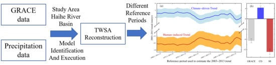
:Terrestrial water storage (TWS) can be influenced by both climate change and anthropogenic activities. While the Gravity Recovery and Climate Experiment (GRACE) satellites have provided a global view on long-term trends in TWS, our ability to disentangle human impacts from natural climate variability remains limited. Here we present a quantitative method to isolate these two contributions with reconstructed climate-driven TWS anomalies (TWSA) based on long-term precipitation data. Using the Haihe River Basin (HRB) as a case study, we find a higher human-induced water depletion rate (−12.87 ± 1.07 mm/yr) compared to the original negative trend observed by GRACE alone for the period of 2003–2013, accounting for a positive climate-driven TWSA trend (+4.31 ± 0.72 mm/yr). We show that previous approaches (e.g., relying on land surface models) provide lower estimates of the climate-driven trend, and thus likely underestimated the human-induced trend. The isolation method presented in this study will help to interpret observed long-term TWS changes and assess regional anthropogenic impacts on water resources.
1. Introduction
Terrestrial water storage (TWS) is the sum of all forms of water storage over land surfaces, which plays a key role in the global and regional hydrological cycle [1,2,3]. TWS varies on a wide range of temporal and spatial scales, and exerts important effects upon the Earth’s climate system [4,5,6]. After the launch of the Gravity Recovery and Climate Experiment (GRACE) satellites in 2002, many studies have quantitatively estimated the TWS or groundwater storage (GWS) changes using GRACE data in global and regional basins [7,8,9,10]. GRACE satellites can derive global monthly temporal gravity fields with a spatial resolution of ~300 km, which can be further used to estimate water storage changes over land when other mass change effects are removed from the gravity fields [11,12]. However, the lack of in situ observations limits our knowledge of the relationship between natural climate variability, and human activity impacts upon terrestrial water systems [13,14,15,16].
Water resources in basins are mainly influenced by climate changes and anthropogenic activities [14]. Assessing changes in water storage on the global scale under the impact of climate variability and human activity has drawn great attention to the growing water scarcity around the world [15,17,18,19,20,21,22,23].
On one hand, the climatic fluctuations in ocean and atmosphere, such as El Niño–Southern Oscillation (ENSO), resulting from the large-scale ocean–atmosphere interactions over the equatorial Pacific [24], can strongly affect global water storage by influencing precipitation patterns [25,26,27]. During the warm phase of ENSO (i.e., El Niño), heavy rains generally occur in South America, while droughts occur in Southeast Asia and Australia. On the contrary, during the cold phase of ENSO (i.e., La Niña), heavy rains occur in Southeast Asia and Australia, while droughts occur in Southwestern USA and the West Coast of South America. Other climatic fluctuations, e.g., Pacific Decadal Oscillation (PDO), Indian Ocean Dipole (IOD) and North Atlantic Oscillation (NAO) also impact TWS anomalies (TWSA) at different temporal and spatial scales [28,29]. On the other hand, due to the increasing water resource management and consumption all around the world, impacts of anthropogenic activities on water storage become more important, and should be taken into account in the hydrologic cycle and modeling [30,31]. Impacts of direct human activities could be through water withdrawal [32,33,34], the building of reservoirs [35,36], or land use and land cover change [37].
Some previous studies have focused on analyzing the relative contribution of TWSA from natural and anthropogenic effects [13,14,17,38,39]. For instance, Yi et al. [39] estimated an anthropogenic TWS depletion estimate of −187 ± 38 km3/yr in Asia by using a linear relationship between variations in precipitation anomalies and water storage fluxes. Huang et al. [14] isolated the human-induced TWSA by subtracting climate-driven TWSA simulated by models from GRACE-observed TWSA. As GRACE can detect the total TWS changes affected by both climate variability and human activities, whereas land surface model (LSM) simulations generally represent the climate-related TWS changes in most cases. Felfelani et al. [13] quantified the human-induced TWSA by calculating the difference between the two hydrological models, in which human impacts were considered in one model, but not included in the other one. However, there are some limitations and uncertainties in terms of modeling and forcing data. For example, Yi et al. [39] assumed that the anthropogenic component is constant over time, and the climate-driven effect is zero from 1979 to 2015, and they analyzed both impacts on the annual scale. A systematic difference between various precipitation-forcing data was also highlighted [39]. Felfelani et al. [13] also found that the TWSA trend uncertainty caused by the errors in forcing datasets was as high as the TWSA trend differences resulting from different hydrological models. Moreover, global hydrological models and land surface models may exhibit large biases in TWSA amplitude [8,20].
Here we quantify the contribution of climate-driven TWSA and its trend based on the reconstruction of long-term climate-driven water storage variations using one decade of GRACE observations and a more than four-decade precipitation dataset, and further evaluate the human-induced TWSA by removing the climate-driven TWSA from the GRACE-derived TWSA. We employ the information from the current GRACE record and avoid the difficulties of using hydrological models by using a statistical approach. The upper and lower bounds of the climate-driven TWSA trend (TrendCD) and human-induced TWSA trend (TrendHI) are estimated based on a relatively long time period of reconstructed, climate-driven TWSA time series.
2. Materials and Methods
2.1. Study Area
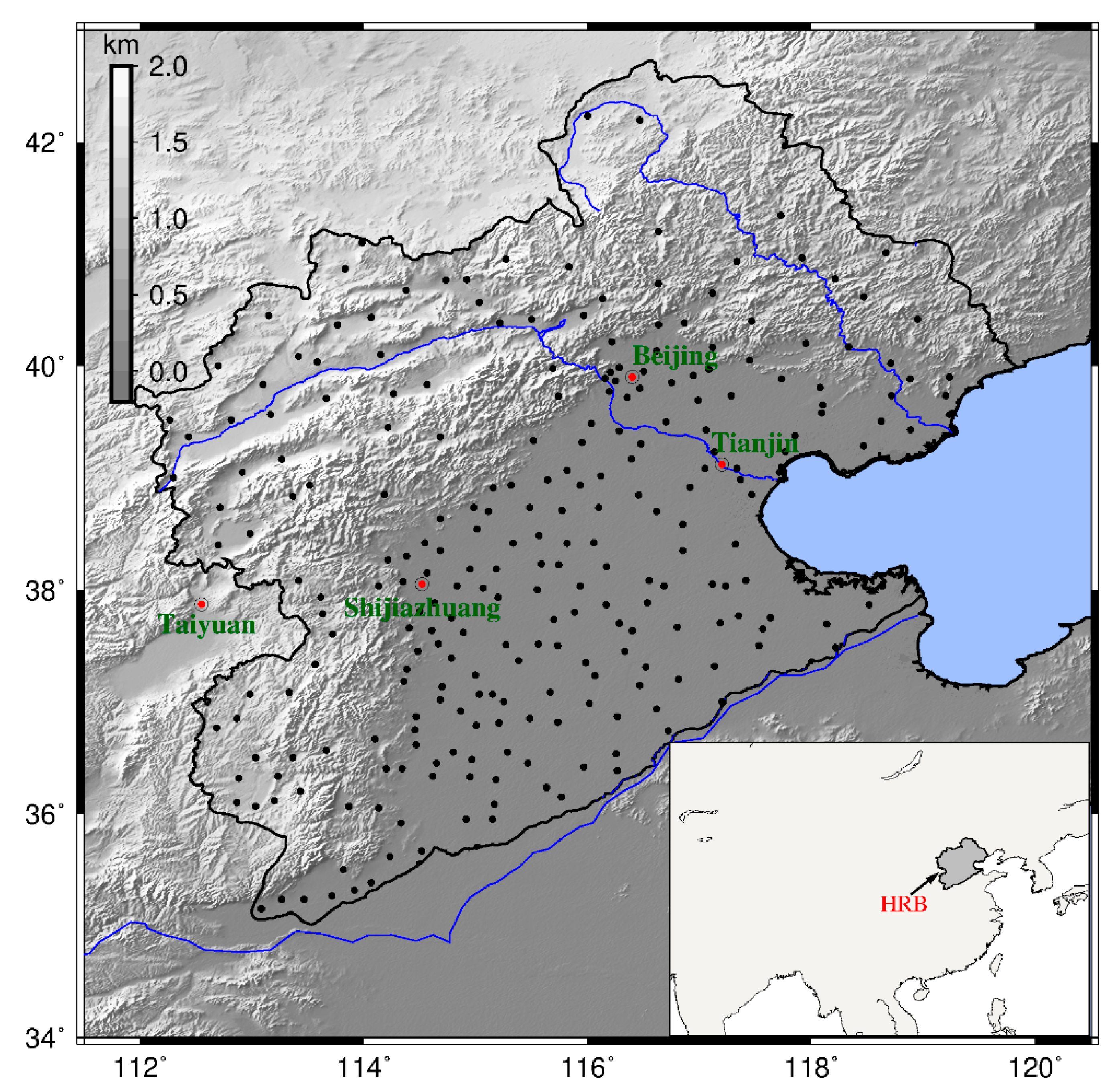
The Haihe River Basin (HRB) is selected as a case study, which is located in North China (~320,000 km2; Figure 1a). The HRB has a total population of ~124 million, including Beijing, Tianjin, and most of the area of Hebei, which is the political, economic and cultural center of China (Figure A1). As a major grain-producing region in China, it produces 10% of China’s total grains [40]. The major crops in this area are winter wheat and summer maize.
In this basin, the mean annual precipitation is ~530 mm/yr from 1961 to 2013. The runoff is mostly generated in the mountainous regions; its mean runoff in the hydrologic control station of Haihezha is only 0.82 km3/yr from 1960 to 2010 [41]. The water consumption is concentrated on the plain region, and it contains the main agricultural areas, industries and cities.
Agriculture depends largely on groundwater exploitation in the HRB, which is similar to the High Plains in the USA and northwest India, and it has become the major groundwater depletion areas around the world [42]. The GWS suffers a prolonged declining trend of −17.8 ± 0.1 mm/yr during 1971–2015 in the North China Plain [43], which covers most of the region of the HRB.
In recent years, with the launch of the GRACE satellite, the water depletion in the HRB has been a research hotspot, given its significant depletion rate and important role in China [43,44,45,46,47,48,49]. Most of the water depletion is caused by agricultural irrigation in the HRB [17,44,50]. Previous study has tried to quantify the climate-driven and human-induced TWSA in the HRB. For example, Yi et al. [39] found a human-induced TWSA trend of −8.4 ± 0.9 km3/yr in the HRB from 2003 to 2014 based on a linear regression of annual precipitation anomalies against GRACE-derived TWSA. In this study, we aim to isolate climate-driven and human-induced contributions to GRACE-derived TWSA in the HRB on the basis of the statistical reconstruction method.
2.2. GRACE Data
The GRACE mascon product is provided by the Center for Space Research (CSR); the University of Texas at Austin is used (http://www2.csr.utexas.edu/grace/). CSR mascons (CSR-M) are provided with a 0.5-degree spatial resolution. The C20 replacement, degree 1 corrections and the glacial isostatic adjustment (GIA) correction have been applied to CSR-M, similar as standard processing for spherical harmonic products. More details about the mascon product can be found in Save et al. [51]. This dataset has been used in several studies to derive global and regional TWSA estimates [10,20,33,49].
We also use two other mascon solutions for intercomparison of reconstruction and trend estimation: one is the Jet Propulsion Laboratory mascons (JPL-M) [52], and the other is the Goddard Space Flight Center mascons (GSFC-M) [53]. The JPL-M data is also processed based on the Level-1 GRACE observations, and the same corrections are applied as CSR-M. The JPL-M uses a priori constraints to estimate global monthly gravity fields in terms of 4551 equal-area, surface spherical-cap mass-concentration functions to minimize the effect of measurement errors [52]. The gain factors are not applied in our study, since they are not suitable to quantify trends from the JPL-M [52]. GSFC-M uses different least squares constraint strategies to develop its mascon solutions relative to JPL-M [53].
The GSFC solution uses many more and much smaller mascons than JPL-M to represent global mass changes. We extract the mascon grids in our study area. The GRACE gridded data used in this study covered a total period of 124 months (January 2003 to December 2013).
2.3. Precipitation Data
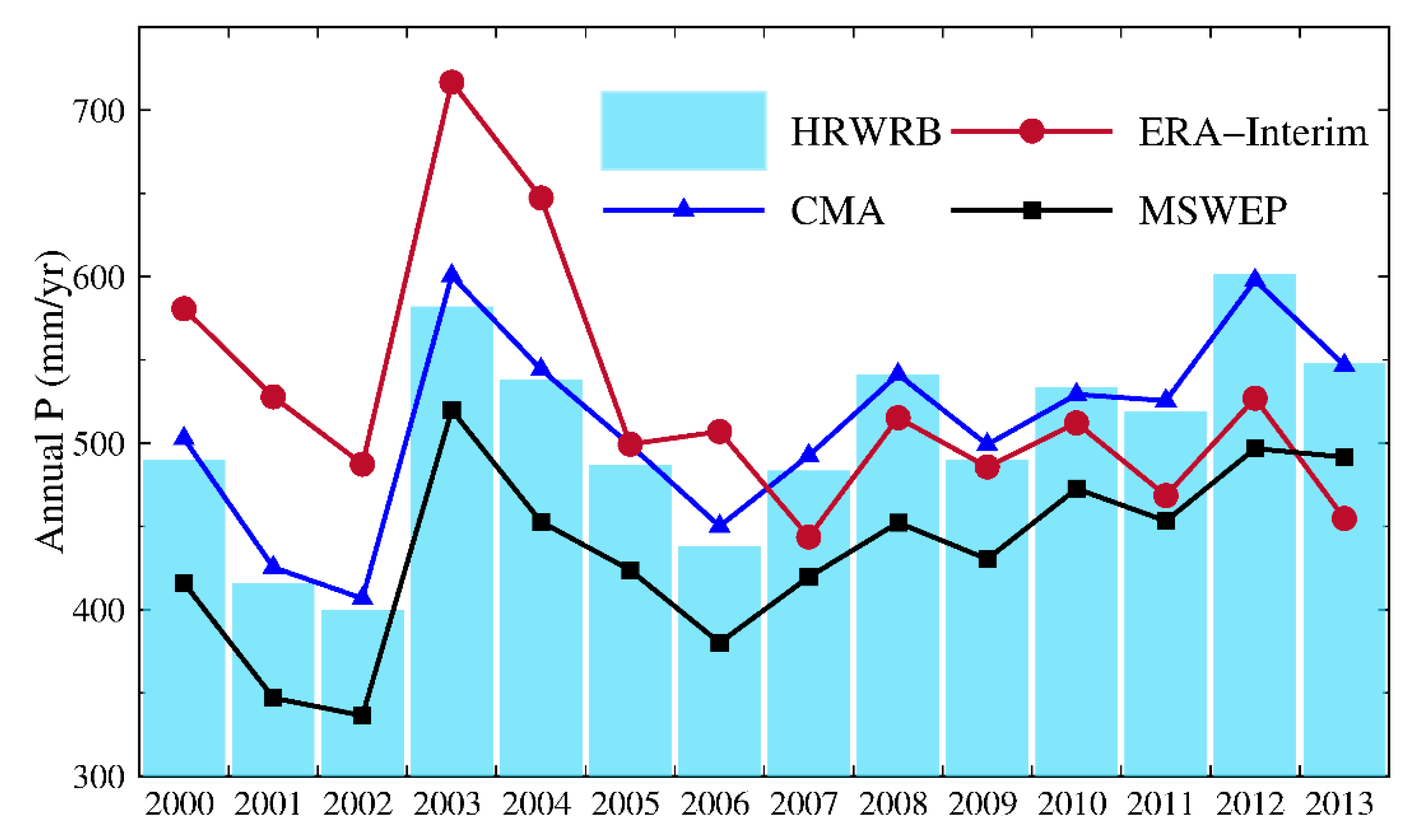
Gridded daily precipitation data over the study region are obtained from the China Meteorological Administration (CMA) for the period of 1961–2013. The reconstruction period is from 1967 for discarding six spin-up years as suggested by Humphrey et al. [54]. The gridded data were obtained by partial thin plate smoothing splines interpolation of precipitation observations from 2472 weather stations with daily temporal resolution and 0.5° × 0.5° spatial resolution over the whole of China, and 258 weather stations were used in the HRB (Figure A1). These datasets were validated with gauge observations by generalized cross-validation, Root Mean Square Error (RMSE), absolute error and relative error [55]. Humphrey and Gudmundsson [56] highlighted that the quality of the reconstruction is heavily dependent upon the quality of the input precipitation forcing. Two global precipitation forcing datasets applied by Humphrey and Gudmundsson [56] are also used to compare with the CMA precipitation dataset, including the European Centre for Medium-Range Weather Forecast (ECMWF) re-analysis (ERA-Interim) dataset and the multi-source weighted-ensemble precipitation dataset (MSWEP). We validate these three precipitation datasets with annual mean precipitation statistics from the Haihe River Water Resources Bulletin (HRWRB) (http://www.hwcc.gov.cn/hwcc/wwgj/xxgb/szygb/). The statistics from HRWRB are more reliable due to more precipitation data from local meteorological stations included, but only annual mean precipitation statistics over the whole HRB are available. The comparison with statistics from HRWRB indicates that the CMA precipitation data used in this study are more reliable than those from ECMWF and MSWEP over the HRB (Text A1, Figure A2, Table A1), consistent with previous findings from Pan et al. [57].
2.4. Land Surface Models
The Global Land Data Assimilation System (GLDAS) Noah is also used to estimate climate-related TWSA. In GLDAS LSMs, the TWS is the sum of soil moisture content and snow water equivalent. The GLDAS LSMs were developed by the National Aeronautics and Space Administration (NASA) and the National Oceanic and Atmospheric Administration (NOAA). Constrained by ground- and space-based observations, the GLDAS LSMs can simulate optimal fields of land surface states and fluxes [58]. The data has a 1-degree spatial resolution over global land, with a monthly temporal resolution.
Climate Prediction Center (CPC) global monthly soil moisture data is also used to estimate climate-related TWSA [59]. The dataset has a 0.5-degree spatial resolution from 1948 to the present. The CPC dataset contains monthly averaged soil moisture water height equivalents.
2.5. Climate-Driven Water Storage Variability
Humphrey et al. [54] proposed a data-driven statistical model where precipitation is filtered using an exponential decay function that is optimized to yield the best correlation with the GRACE-observed TWSA [60]. Here we conduct our study based on the reconstructed climate-driven TWSA. However, we did not consider interannual temperature anomalies [33], since there are non-significant correlation coefficients between interannual temperature and TWSA in the HRB [60]. Different methods with and without considering temperature anomalies [33,54], as well as a new method proposed by Humphrey and Gudmundsson [56], were tested, but results indicate that differences among these methods are negligible in the HRB (Text A2, Figure A3, Table A2, Table A3). The climate-driven TWSA is formulated as follows:
where TWSArec is the reconstructed, deseasoned and detrended TWS variations; corresponds to the deseasoned and detrended monthly precipitation. The parameters τ and β are calibrated against the monthly TWSA derived from deseasoned and detrended GRACE-observed TWSA. We apply this method on the basin scale, which is different from that of the grid scale considered in Humphrey et al. [54].
2.6. Quantifying the Contributions of Climate-Driven and Human-Induced TWSA Trends
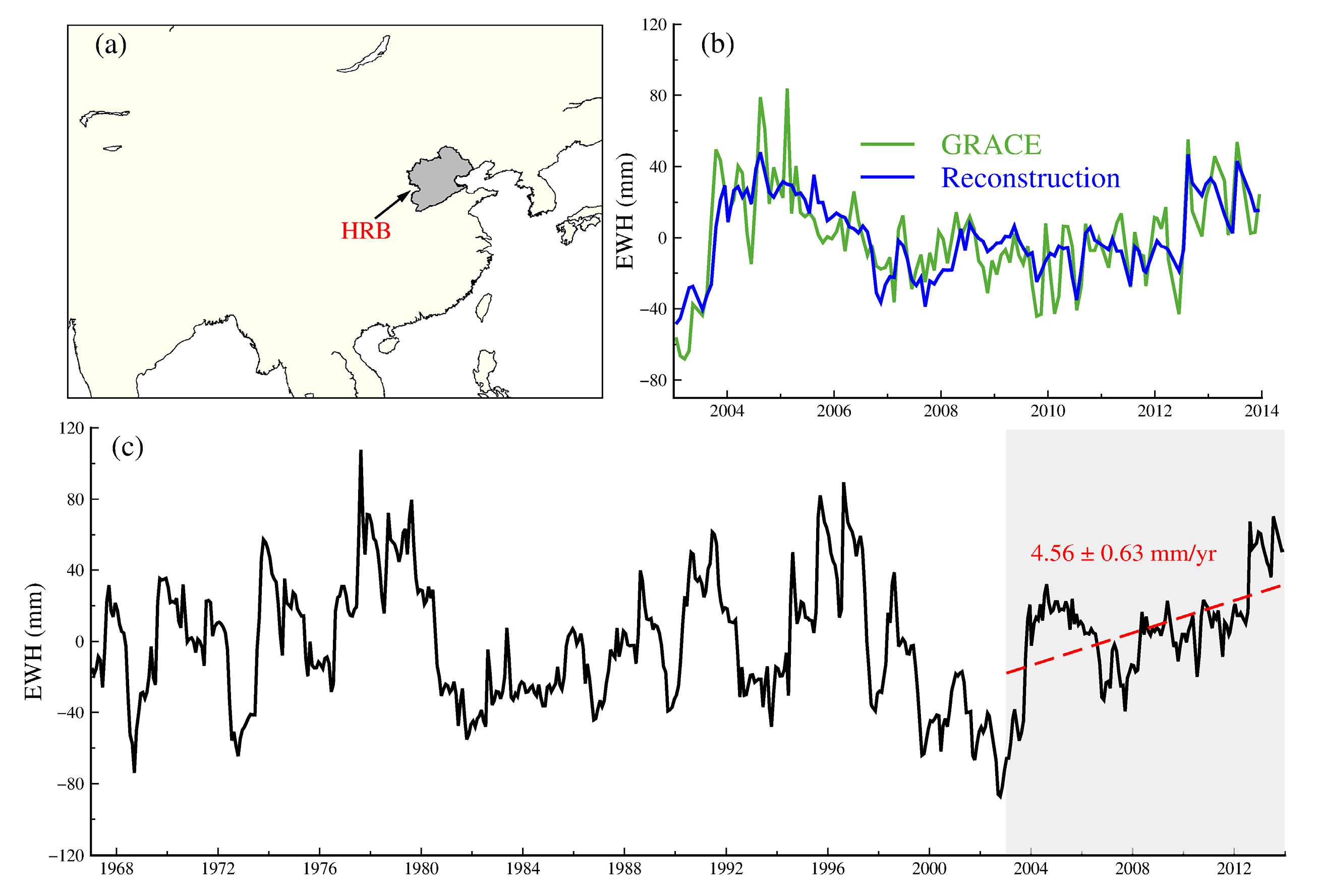
As shown in Figure 1c, we reconstruct the long-term, climate-driven TWSA from January 1967 to December 2013. The linear trend of TWSA for the reference period or the reconstruction period (i.e., 1967.01–2013.12) is zero, according to the definition of reconstruction [54], but the TWSA time series for the study period (i.e., 2003.01–2013.12) have a trend of 4.56 ± 0.63 mm/yr (expressed as: ). It should be noted that the trend of reconstructed climate-driven TWSA for the study period will vary corresponding to different reference periods (see Table 1 and Movie S1). We further estimate an upper and lower bound of the climate-driven trend by considering as many possible reference periods. The mean climate-driven trend is estimated as Equation (2).
where is the mean climate-driven trend, ith is the start year/month of the reference period (i.e., 1967.01, 1967.02, 1967.03, ⋯, 1993.12), and n represents the number of considered reference periods, equivalent to the number of months from January 1967 to a suitable time (i.e., December 1993 and n = 324, see Table 1). We select December 1993 to December 2013 as the last reference period, so that the reconstruction period can be at least 20 years or longer. The superscript of , i.e., 2003–2013, represents the study period to estimate the climate-driven trend. The subscript of represents the reference period used for reconstruction. The climate-driven trend estimated under a longer reconstruction period tends to be more stable, as it is less influenced by extreme precipitation anomalies in some years.
Then, the human-induced TWSA trend is estimated as follows:
where TrendHI is the trend of human-induced TWSA, TrendGRACE is the total trend of GRACE-derived TWSA, and TrendCD is the climate-driven trend estimate.
2.7. Error Estimation
The uncertainty of TWSA is estimated following the approach used in Landerer and Swenson [8] and Scanlon et al. [10]. Details can be found in the supporting information in Scanlon et al. [10]. The uncertainty of is estimated as the formal error of trend estimate by applying least squares to fit a linear trend to the constructed climate-driven TWSA time series from 2003 to 2013 using the reference period of ith-201312 [33,61]. The error of is estimated as the combination of the mean formal error of different and the standard deviation (STD) of different trend estimates considering all the different reference periods. The equation is as follows:
where is the error of , is the mean formal error of different , and represents the STD of different trend estimates.
The error of the is estimated using conventional error propagation as Equation (5), with representing the error of the GRACE TWSA trend.
The uncertainties of annual climate-driven and human-induced TWSA are also estimated. We first estimate the uncertainties of the monthly TWSA time series, then the uncertainty of reconstructed TWSA, which is estimated by the root mean square error (RMSErec-obs) between reconstructed and GRACE observations [54], and then variations of monthly TWSA (var) for every month which are estimated from the STDs of 324 climate-driven TWSA time series (see Section 2.6). Thus, the uncertainties of annual climate-driven TWSA can be estimated as follows:
where is the uncertainty of annual climate-driven TWSA.
The uncertainty of annual human-induced TWSA is estimated with conventional error propagation considering both annual uncertainties of GRACE and climate-driven TWSA, similar to Equation (5). It should be noted that the uncertainties provided in this study are provided as 68.3% confidence intervals.
3. Results
3.1. Trend of Climate-driven and Human-Induced TWSA
As shown in Figure 1b, our reconstructed time series of TWSA agree well with the GRACE results, with a high correlation coefficient (R) of 0.79 and Nash-Sutcliffe Efficiency (NSE) of 0.41. The RMSE of two time series of TWSA is 1.6 cm (Table A2), in the same level of GRACE errors, which also indicates the reliability of our reconstructed results.
As shown in Figure 1c, although the trend of reconstructed time series of TWSA from 1967 to 2013 is zero according to the definition of reconstruction method, there are significant fluctuations on interannual to decadal time scales. We compute the trend of reconstructed climate-driven TWSA for the period of 2003–2013 using different reference periods as explained by Equation (2) in Section 2.6 (i.e., , , ⋯,). Further, the time series of human-induced trends of TWSA for the period of 2003–2013 are estimated by removing climate-driven TWSA trends from GRACE-derived TWSA trends following Equation (3).
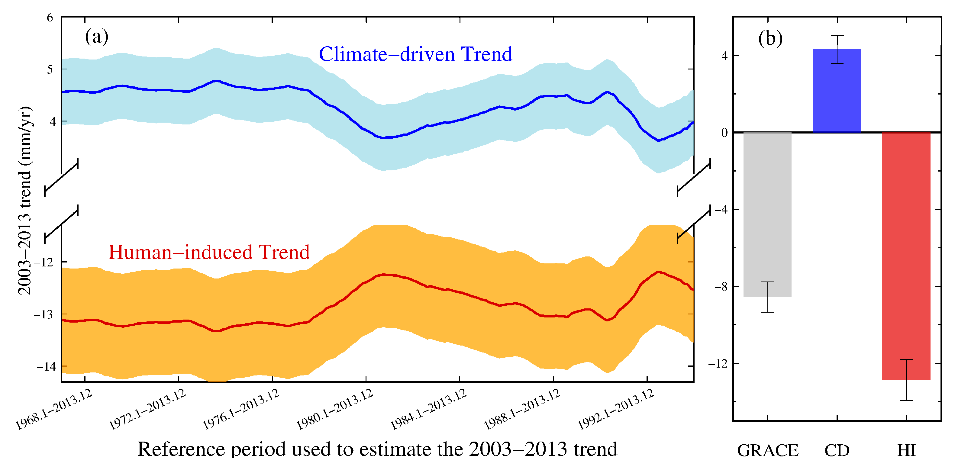
The GRACE-derived TWSA trend from January 2003 to December 2013 is −8.56 ± 0.79 mm/yr (i.e., −2.74 ± 0.25 km3/yr), while the TrendCD ranges from 3.63 to 4.77 mm/yr depending on the various reference periods (Figure 2, Text A3). The mean TrendCD is estimated to be 4.31 ± 0.72 mm/yr (i.e., 1.38 ± 0.23 km3/yr). The TrendCD time series show some fluctuations over the different reference periods, but their standard deviation is only 0.34 mm/yr. As shown in Figure 2a, when the reconstruction period becomes longer than 37 years (i.e., the starting year ranges from 1967 to 1977), the trend estimates tend to become more stable.
3.2. Interannual Variations of TWSA
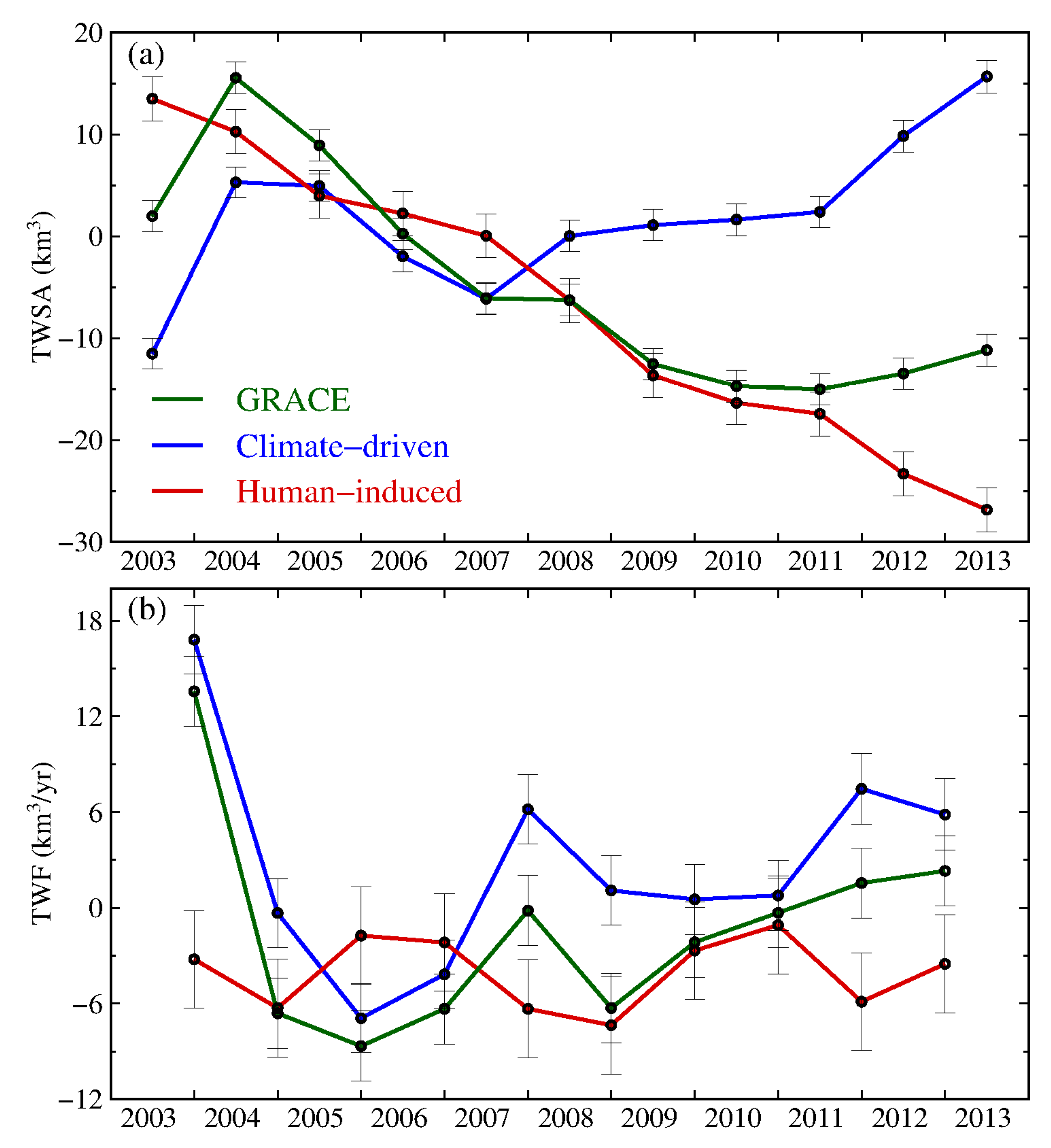
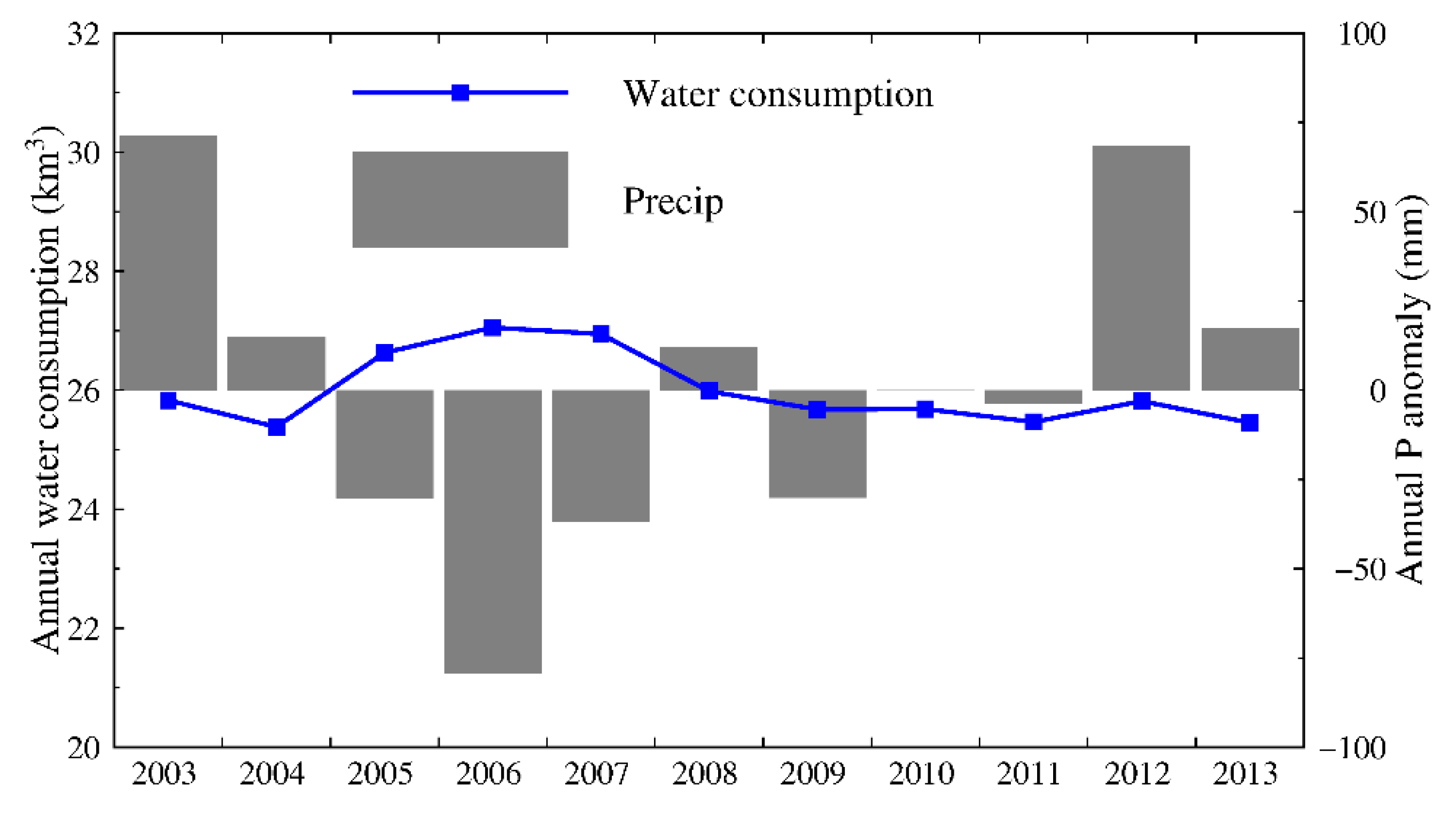
To better illustrate the year-to-year variability of TWSA, monthly GRACE-derived, climate-driven and human-induced TWSA are averaged to annual means (Figure 3a). The climate-driven TWSA increased with fluctuations, while the human-induced TWSA continuously decreased, indicating a continuous human-induced water mass loss. The climate-driven TWSA decreased from 2004 to 2007 and increased continuously after 2007, which is consistent with year-to-year precipitation anomalies during the same time period (Figure A4). However, the human-induced TWSA shows a long-term continuous decrease without significant interannual variability, indicating a stable negative effect on water storage from anthropogenic activities (Figure 3a). As the leading factor of human activities, the long-term extensive water consumption with a rate of ~26 km3/yr based on the statistics from HRWRB causes the continuous decrease of human-induced TWSA (Figure A4).
Further, the year-to-year terrestrial water fluxes (TWF) are calculated as the difference between annual mean TWSA in two consecutive years. As shown in Figure 3b, the interannual GRACE TWF are dominated by the climate-driven TWF. The climate-driven TWF between 2003 and 2004 is 16.80 ± 2.15 km3/yr, corresponding to the positive precipitation anomaly in 2003 and 2004. The abnormal negative precipitation anomaly in 2006 (i.e., −79.14 mm relative to average precipitation of 1961 to 2013, Figure A4) corresponds to minimum TWF (−6.92 ± 2.15 km3/yr) between 2005 and 2006. The human-induced TWF are all in negative values, ranging from −6.28 ± 3.06 to −1.09 ± 3.06 km3/yr.
4. Discussion
4.1. Comparison of Different GRACE Solutions and Methods
The method to separate contributions of climate-driven and human-induced activities in this study is also applied by using JPL-M and GSFC-M. As shown in Table 2, the GRACE-derived TWSA trend from JPL-M is significantly larger than those from CSR-M and GSFC-M. Scanlon et al. [10] also found larger trends in JPL-M after a global evaluation of different GRACE solutions, especially in medium and small basins (≤500,000 km2), which can be caused by the different processing strategy and a priori constraints used in JPL-M [52,62]. The climate-driven trend estimates from CSR-M, GSFC-M and JPL-M are 4.31 ± 0.72, 3.35 ± 0.66, and 5.66 ± 0.95 mm/yr, respectively. The mean value of the three estimates is 4.44 mm/yr, and it is closer to the CSR-M estimate, which we used finally in this study. Due to the positive trends of climate-driven TWSA during 2003–2013, the negative trends of the human-induced TWSA are all larger than those of GRACE-derived total TWSA.
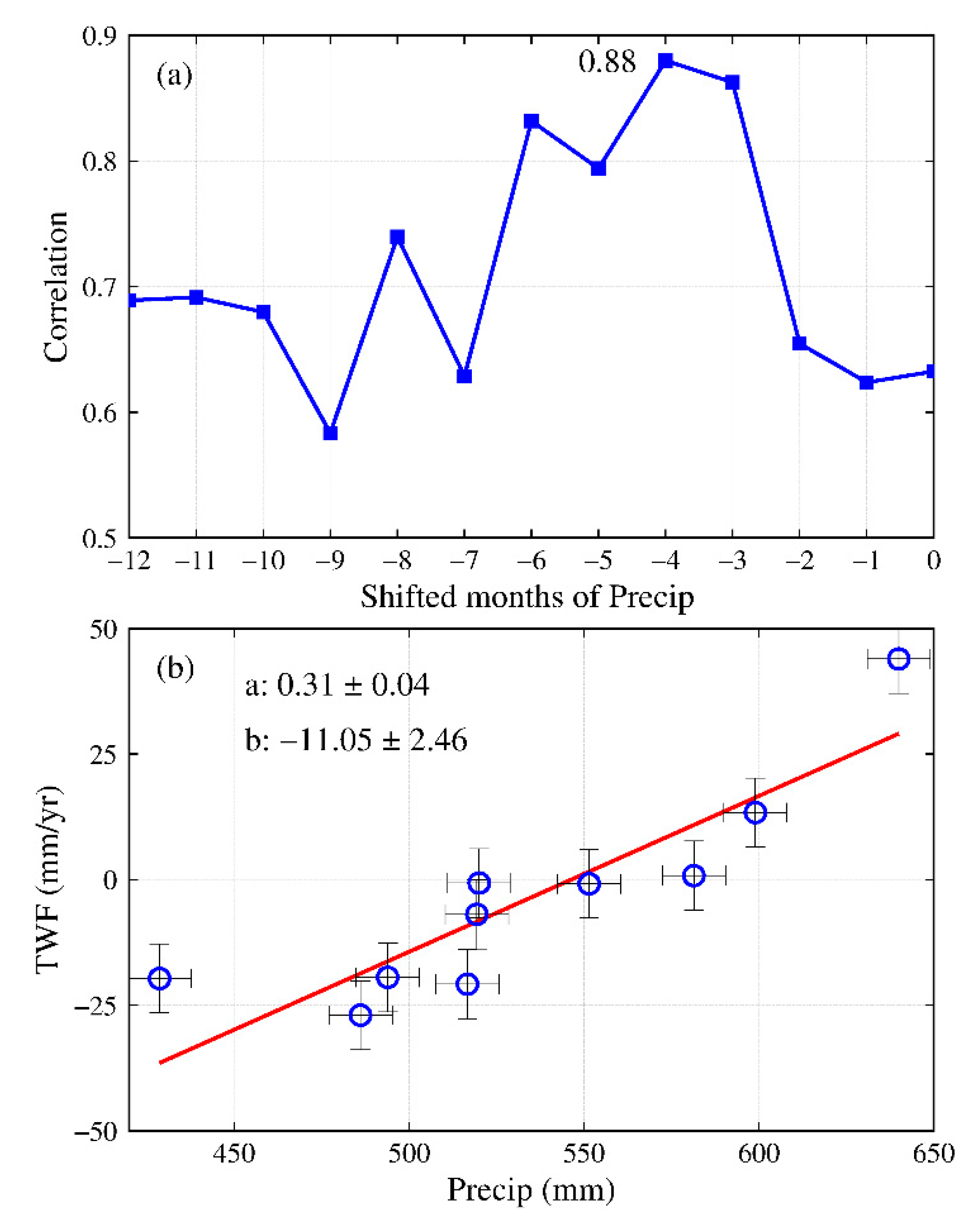
We reproduce the method of Yi et al. [39] by assuming a simple linear relationship between annual precipitation anomalies and annual TWF (Figure A5). The TrendHI estimated by this method is −11.05 ± 2.46 mm/yr, agreeing reasonably well with our TrendHI estimate within uncertainties (Table 2). Note that only precipitation anomalies and TWF on an annual scale can be used to establish a reasonable linear relationship between them in this method. However, in our data-driven reconstruction method, a more complicated decayed response of TWSA to daily precipitation is considered [54].
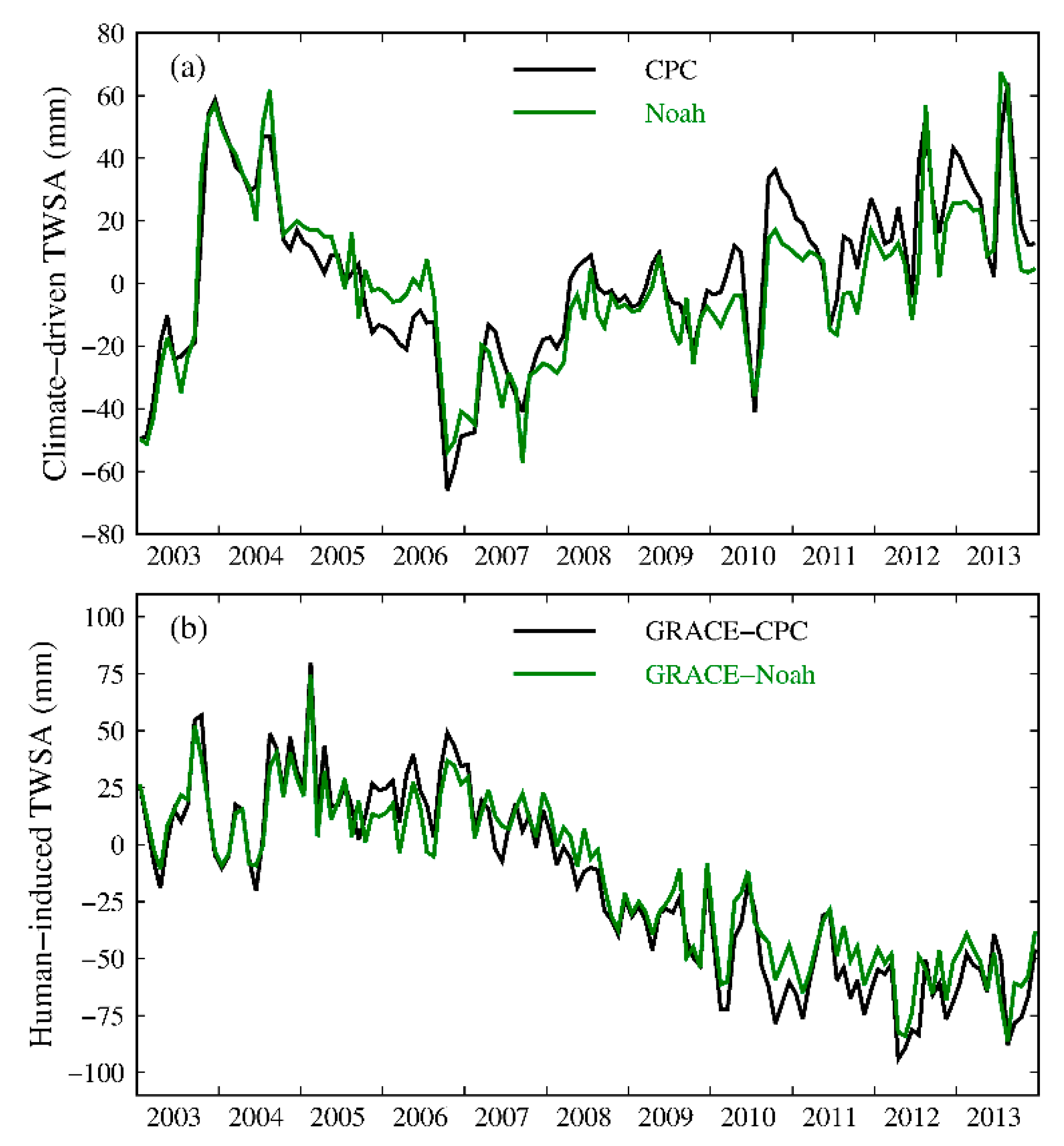
We also follow the method of Huang et al. [14], who take the LSM simulations as the climate-related TWSA. The two climate-driven TWSA time series are relatively similar (Figure A6) in the HRB. The corresponding TrendCD from the Noah and CPC models are 1.09 ± 0.70 and 2.48 ± 0.69 mm/yr, respectively, during 2003–2013 (Table 2). The increased TWSA from LSMs are consistent with the positive climate-driven TWSA trend reconstructed in this study. However, climate-driven TWSA trends estimated by LSMs appear smaller than our estimates. This finding is consistent with a recent study indicating that the amplitude of TWSA trends is systematically underestimated in LSMs (Scanlon et al. 2018), partly because of missing storage compartments such as lakes and aquifers which, on the other hand, are implicitly included in our data-driven reconstruction method. Further, human-induced TWSA time series are estimated by subtracting model-simulated, climate-driven TWSA from GRACE-derived TWSA. The corresponding TrendHI estimates based on the Noah and CPC models are −9.65 ± 1.06 and −11.04 ± 1.05 mm/yr, respectively (Table 2), which are smaller compared to our estimates using the data-driven reconstruction method due to the underestimation of climate-driven TWSA in LSMs.
4.2. Impact of Annual Precipitation Trend
The intrinsic trend in annual precipitation could also contribute to the changes of TWS, as over the Tibetan Plateau in China [17,63], northern North America, Tropical western Africa and Northern Congo [17]. In this study, we assumed that the long-term climatological precipitation remains stable over the reference period, so the trends of the time series of precipitation and climate-driven TWSA are zero over the reference period. In fact, long-term annual precipitation trend may cause an increase or decrease of TWS. In other words, the long-term climate-driven TWSA trend might not be zero.
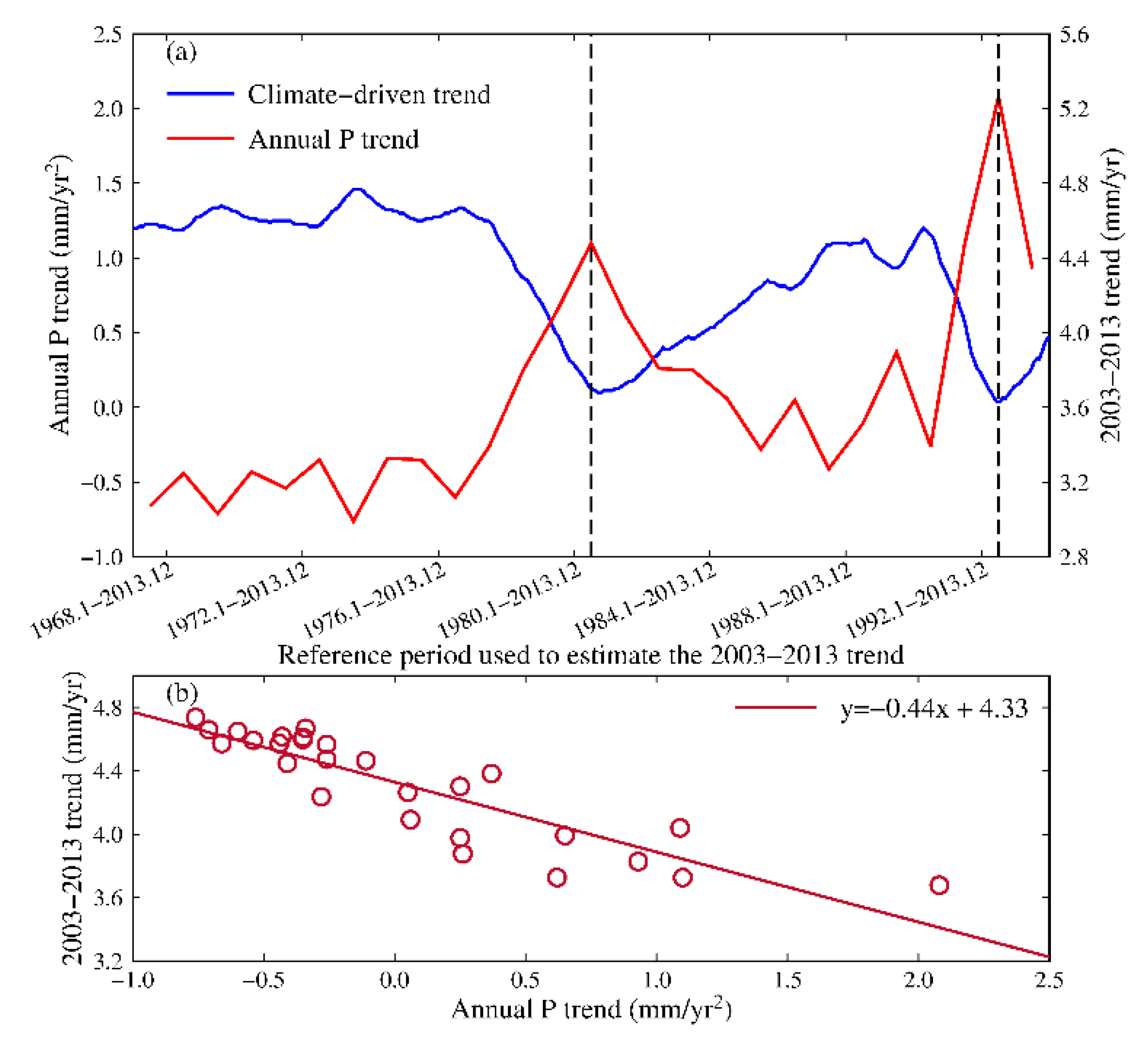
We examined the trend of annual precipitation for different reference periods (i.e., 1967–2013, 1968–2013, ⋯, 1993–2013) using the Mann-Kendall (M-K) trend test (Figure 4a). There are two significant annual precipitation trends during 1980–2013 and 1992–2013 corresponding to the two low values of estimates (Figure 4a), which indicates the impact of annual precipitation trend on the estimation. The precipitation trend remains stable for the reference periods from 1967–2013 to 1977–2013 (Figure 4a), so the estimates are also stable during these reference periods (Figure 2a). A simple linear regression was further performed between annual precipitation trends (predictor) and estimates (dependent variable) during different reference periods (Figure 4b). The regression coefficient shows that the is 4.33 ± 0.63 mm/yr when the annual precipitation trend is zero (Table 2), which is consistent with our estimate. Here we assume that the long-term, climate-driven TWSA trend is zero when the annual precipitation trend is zero.
In addition, we also check the TrendCD and TrendHI estimates by removing the annual precipitation trend before reconstruction. The trend of the annual precipitation during 1961–2013 is found to be −0.87 mm/yr2 based on the M-K trend test, but not significant (p > 0.1). Nevertheless, we still consider its contribution as follows. We first removed the annual precipitation trend by adding the corresponding amount of precipitation in the daily precipitation time series, so the annual precipitation trend for the period of 1961–2013 is close to zero after this processing. The detrended daily precipitation time series are further used to reconstruct the climate-driven TWSA. Finally, the TrendCD and TrendHI are estimated to be 4.31 ± 0.71 and −12.87 ± 1.07 mm/yr, respectively (Table 2). There is almost no difference between these estimates and the foregoing trend estimates using the original precipitation. Thus, we can conclude that the trend of annual precipitation has no obvious influence on our TrendCD and TrendHI estimates in the HRB.
However, it is worth noting that special attention might be required when applying the method to a region with a significant annual precipitation trend during the reconstruction period. Technically, the potential impact of a precipitation trend can be tested by applying regression analysis between annual precipitation trends and TrendCD estimates proposed in this study.
5. Conclusions
In this study, we use a data-driven reconstruction method to quantify the contributions of climate and anthropogenic activities to water storage changes. This method takes advantage of the information from GRACE and in situ precipitation data. The HRB, suffering a long-term water depletion, is taken as a case study. Although the apparent rate of TWSA in the HRB measured by GRACE is −8.56 ± 0.79 mm/yr over 2003–2013, we estimate a climate-driven TWSA trend of 4.31 ± 0.72 mm/yr (i.e., 1.38 ± 0.23 km3/yr) due to the wet period in the past decade relative to the climate of the past half century. Therefore, the human-induced TWSA trend is −12.87 ± 1.07 mm/yr (i.e., -4.12 ± 0.34 km3/yr) for the period of 2003–2013, which indicates that the human-induced water depletion in the HRB is more serious (i.e., ~50% larger) than that estimated by GRACE observations alone.
While annual climate-driven TWSA shows some fluctuations with a positive trend, prolonged anthropogenic water abstractions lead to a continuous decrease in TWSA. Although the climate-driven TWSA increase partially compensates the human-induced water depletion in the case of the HRB, it should be noted that there might also be opposite cases in which a negative climate-driven TWSA trend along with an existing anthropogenic TWSA depletion will exacerbate the total water loss in some regions of the world.
The potential effect of the long-term annual precipitation trend in the HRB is also investigated, with the results showing that it has almost no effect in the HRB. However, we recommend that caution should be exercised in regions with the significant precipitation trend when applying the reconstruction method.
The method presented in this study provides a way to isolate the individual contribution of climate variability or human activities to decadal water storage changes observed by GRACE, which would definitely benefit the interpretation of observed net changes in water storage and water resources management. Our results indicate that although the climate-driven water storage varies corresponding to the precipitation changes, the water storage variations due to anthropogenic activities show a continuous decreasing rate in the HRB, which highlights the possible underestimation or overestimation of actual human-induced water depletion in other regions of the world when GRACE data alone was used to quantify regional water storage changes.
Author Contributions
Conceptualization, Y.Z., W.F. and V.H.; methodology, Y.Z., W.F. and V.H.; investigation, Y.Z.; data curation, Y.Z.; writing—original draft preparation, Y.Z. and W.F.; writing—review and editing, W.F., M.Z. and V.H.; funding acquisition, Y.Z., M.Z. and W.F.
Funding
The research is funded by National Natural Science Foundation of China (41674084, 41774094, 41431070, and 41874095); Fundamental Research Funds for the Central Universities, China University of Geosciences (Wuhan) (G1323519314); Natural Science Fund for Distinguished Young Scholars of Hubei Province, China (Grant No. 2019CFA091); Open Research Fund Program of State Key Laboratory of Geodesy and Earth’s Dynamics (SKLGED2019-2-5-E); and Key Laboratory of Surveying and Mapping Science and Geospatial Information Technology of Ministry of Natural Resources.
Acknowledgments
We would like to acknowledge the NASA Goddard Space Flight Center (GSFC), the Jet Propulsion Laboratory (JPL), and the Center for Space Research (CSR), University of Texas at Austin for providing the GRACE mascon solutions. We also acknowledge the China Meteorological Administration for providing the grid precipitation data. The presented dataset in this study is archived in the Global Change Research Data Publishing and Repository (GCdataPR, http://www.geodoi.ac.cn/WebCn/doi.aspx?Id=1298). The authors thank Fei Li, Haoming Yan, and RAAJ Ramsankaran for their insightful suggestions and comments on the earlier draft of this manuscript.
Conflicts of Interest
The authors declare no conflict of interest.
Appendix A
Text A1. Comparison of Precipitation Forcing Data
Different precipitation forcing data are compared with each other, including daily precipitation from China Meteorological Administration (CMA), the European Centre for Medium-Range Weather Forecast (ECMWF) re-analysis (ERA-Interim) [64] and multi-source weighted-ensemble precipitation dataset (MSWEP) [65]. We compared the four precipitation datasets on the annual scale with the precipitation data from the Haihe River Water Resources Bulletin (HRWRB). The comparison is evaluated with three indices: correlation coefficient (R), Mean Bias Error (MBE) and Root Mean Square Error (RMSE) (Table A1). Results indicate that precipitation data from CMA are more reliable in the HRB, which is in line with Pan’s conclusion [57].
Text A2. Comparison of Different Reconstruction Methods
Results with or without considering the interannual temperature in the reconstruction are shown in Figure A3, which are applied in Humphrey et al. [54] and Zhong et al. [33], respectively. The interannual temperature data are obtained from the ERA-Interim atmospheric reanalysis [64]. A new reconstruction method proposed by Humphrey and Gudmundsson [56] is also taken into comparison. The results are evaluated with three indices: the Nash-Sutcliffe efficiency (NSE) [66], RMSE and R (Table A2, Table A3). The comparison results indicate that the impact of temperature is limited in the HRB. Considering that there is non-significant R between the interannual temperature and TWSA, we choose the method without considering the temperature.
Text A3. A Relatively Conservative Estimate of TrendCD and TrendHI
If we assume the climate-driven trend is zero for the longest reference period (i.e., = 0), then TrendCD is estimated to be 4.56 mm/yr. The subsequent trend time series are used to estimate the upper and lower bounds of TrendCD (Figure 2a). Thus, the upper and lower bounds are 3.63 and 4.77 mm/yr, respectively. This estimate is also close to the previous estimate. Then the TrendHI estimate is −13.12 mm/yr, and its upper and lower bounds are −12.19 and −13.33 mm/yr, respectively.
Figure A1.
Topography map of Haihe River Basin (HRB) which includes locations of precipitation stations (black points), main cities and rivers. The digital elevation model (DEM) data used here is from Yue et al. [67].
Figure A1.
Topography map of Haihe River Basin (HRB) which includes locations of precipitation stations (black points), main cities and rivers. The digital elevation model (DEM) data used here is from Yue et al. [67].

Figure A2.
Time series of annual precipitation from the Haihe River Water Resources Bulletin (HRWRB), China Meteorological Administration (CMA), the European Centre for Medium-Range Weather Forecast (ECMWF) re-analysis (ERA-Interim) and multi-source weighted-ensemble precipitation dataset (MSWEP).
Figure A2.
Time series of annual precipitation from the Haihe River Water Resources Bulletin (HRWRB), China Meteorological Administration (CMA), the European Centre for Medium-Range Weather Forecast (ECMWF) re-analysis (ERA-Interim) and multi-source weighted-ensemble precipitation dataset (MSWEP).

Figure A3.
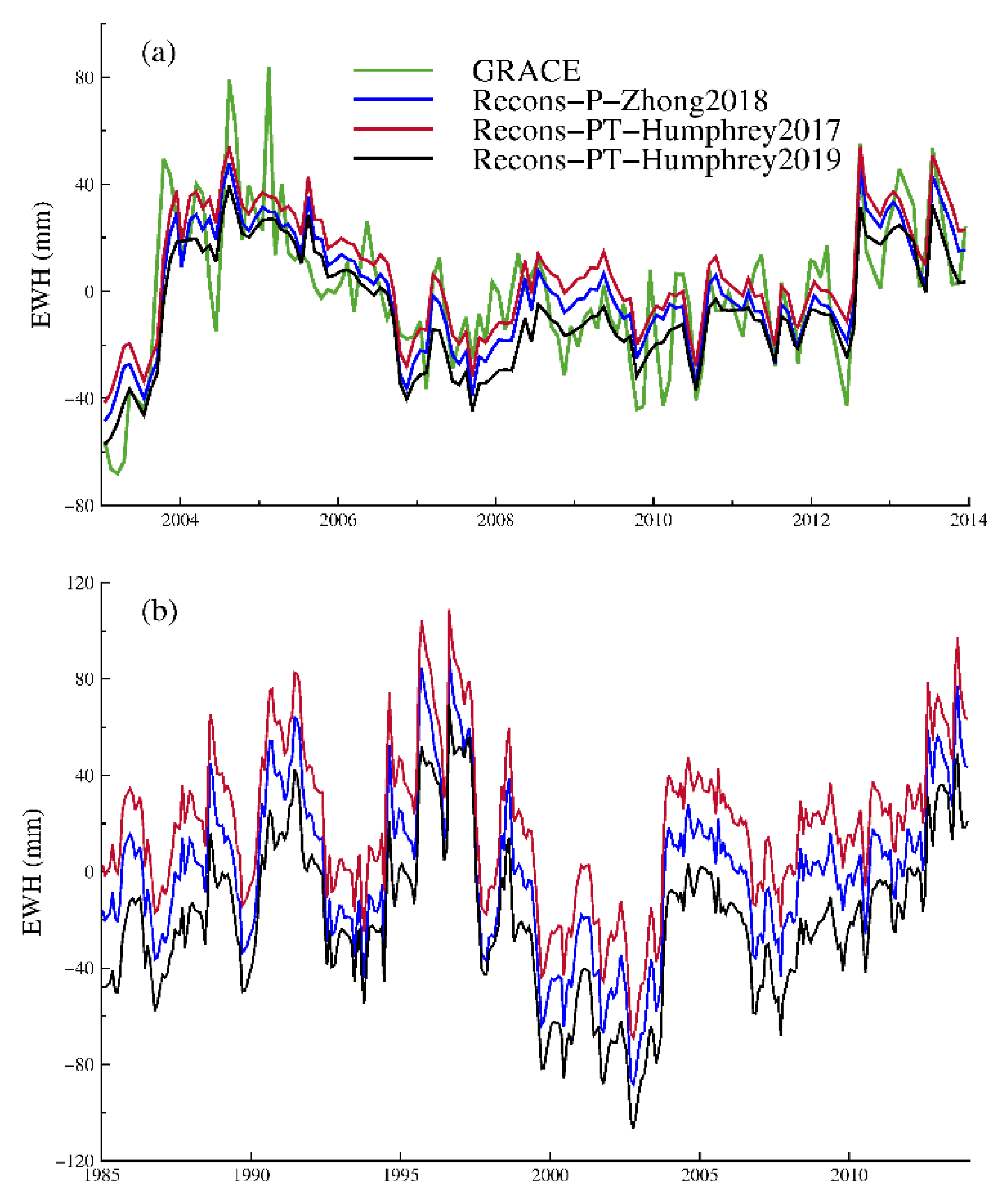
Comparison between GRACE-derived TWSA and different reconstruction methods based on Humphrey et al. [54], Humphrey and Gudmundsson [56] and Zhong et al. [33] for (a) the calibration period from 2003–2013 and (b) the reconstruction period from 1985–2013. Seasonal cycles and the long-term trend have been removed in GRACE-derived TWSA. The curves for Recons-PT-Humphrey2017 and Recons-PT-Humphrey2019 have been offset for clarity.
Figure A3.
Comparison between GRACE-derived TWSA and different reconstruction methods based on Humphrey et al. [54], Humphrey and Gudmundsson [56] and Zhong et al. [33] for (a) the calibration period from 2003–2013 and (b) the reconstruction period from 1985–2013. Seasonal cycles and the long-term trend have been removed in GRACE-derived TWSA. The curves for Recons-PT-Humphrey2017 and Recons-PT-Humphrey2019 have been offset for clarity.

Figure A4.
Annual water consumption and annual precipitation anomalies in the Haihe River Basin from 2003 to 2013.
Figure A4.
Annual water consumption and annual precipitation anomalies in the Haihe River Basin from 2003 to 2013.

Figure A5.
(a) Correlations between terrestrial water fluxes (TWF) and precipitation anomalies, with different shifted months of precipitation; (b) The linear regression between TWF and annual precipitation.
Figure A5.
(a) Correlations between terrestrial water fluxes (TWF) and precipitation anomalies, with different shifted months of precipitation; (b) The linear regression between TWF and annual precipitation.

Figure A6.
(a) Climate-driven TWSA estimates from land surface models (CPC and Noah); (b) Human-induced TWSA estimates from subtracting GRACE TWSA by climate-driven TWSA.
Figure A6.
(a) Climate-driven TWSA estimates from land surface models (CPC and Noah); (b) Human-induced TWSA estimates from subtracting GRACE TWSA by climate-driven TWSA.


Table A1.
Comparison of different precipitation-forcing datasets with precipitation statistics from the Haihe River Water Resources Bulletin on the annual scale.
Table A1.
Comparison of different precipitation-forcing datasets with precipitation statistics from the Haihe River Water Resources Bulletin on the annual scale.
| Method | R | MBE (mm) | RMSE (mm) |
|---|---|---|---|
| CMA | 0.99 | 6.67 | 9.24 |
| ERA-Interim | 0.37 | 21.85 | 76.86 |
| MSWEP | 0.97 | −69.63 | 70.92 |
Table A2.
Comparison of different methods with or without considering the temperature, and a new method from Humphrey and Gudmundsson [56] for the GRACE period. All results are compared with deseasoned and detrended GRACE observations from 2003 to 2013.
Table A2.
Comparison of different methods with or without considering the temperature, and a new method from Humphrey and Gudmundsson [56] for the GRACE period. All results are compared with deseasoned and detrended GRACE observations from 2003 to 2013.
| Method | NSE | RMSE (mm) | R |
|---|---|---|---|
| This study | 0.41 | 16.34 | 0.79 |
| Humphrey et al. [54] | 0.40 | 16.38 | 0.79 |
| Humphrey and Gudmundsson [56] | 0.45 | 16.09 | 0.80 |
Table A3.
Intercomparison of among reconstruction terrestrial water storage anomalies results based on the three methods from 1985 to 2013.
Table A3.
Intercomparison of among reconstruction terrestrial water storage anomalies results based on the three methods from 1985 to 2013.
| Method | NSE | RMSE (mm) | R |
|---|---|---|---|
| This study vs Humphrey et al. [54] | 1.00 | 1.24 | 1.00 |
| This study vs Humphrey and Gudmundsson [56] | 0.96 | 6.50 | 0.98 |
| Humphrey et al. [54] vs Humphrey and Gudmundsson [56] | 0.95 | 7.03 | 0.98 |
References
- Syed, T.H.; Famiglietti, J.S.; Rodell, M.; Chen, J.; Wilson, C.R. Analysis of terrestrial water storage changes from GRACE and GLDAS. Water Resour. Res. 2008, 44. [Google Scholar] [CrossRef]
- Yeh, P.J.F.; Swenson, S.C.; Famiglietti, J.S.; Rodell, M. Remote sensing of groundwater storage changes in Illinois using the Gravity Recovery and Climate Experiment (GRACE). Water Resour. Res. 2006, 42. [Google Scholar] [CrossRef]
- Strassberg, G.; Scanlon, B.R.; Chambers, D. Evaluation of groundwater storage monitoring with the GRACE satellite: Case study of the High Plains aquifer, central United States. Water Resour. Res. 2009, 45. [Google Scholar] [CrossRef] [Green Version]
- Famiglietti, J.S. Remote Sensing of Terrestrial Water Storage, Soil Moisture and Surface Waters. In The State of the Planet: Frontiers and Challenges in Geophysics; American Geophysical Union: Washington, DC, USA, 2013; pp. 197–207. [Google Scholar] [CrossRef]
- Radice, A.; Longoni, L.; Papini, M.; Brambilla, D.; Ivanov, V.I. Generation of a Design Flood-Event Scenario for a Mountain River with Intense Sediment Transport. Water 2016, 8, 597. [Google Scholar] [CrossRef] [Green Version]
- Albano, R.; Mancusi, L.; Abbate, A. Improving flood risk analysis for effectively supporting the implementation of flood risk management plans: The case study of “Serio” Valley. Environ. Sci. Policy 2017, 75, 158–172. [Google Scholar] [CrossRef]
- Feng, W.; Shum, C.K.; Zhong, M.; Pan, Y. Groundwater Storage Changes in China from Satellite Gravity: An Overview. Remote Sens. 2018, 10, 674. [Google Scholar] [CrossRef] [Green Version]
- Landerer, F.W.; Swenson, S.C. Accuracy of scaled GRACE terrestrial water storage estimates. Water Resour. Res. 2012, 48. [Google Scholar] [CrossRef]
- Chen, J.L.; Wilson, C.R.; Tapley, B.D.; Yang, Z.L.; Niu, G.Y. 2005 drought event in the Amazon River basin as measured by GRACE and estimated by climate models. J. Geophys. Res. Solid Earth 2009, 114. [Google Scholar] [CrossRef]
- Scanlon, B.R.; Zhang, Z.Z.; Save, H.; Wiese, D.N.; Landerer, F.W.; Long, D.; Longuevergne, L.; Chen, J.L. Global evaluation of new GRACE mascon products for hydrologic applications. Water Resour. Res. 2016, 52, 9412–9429. [Google Scholar] [CrossRef]
- Tapley, B.D.; Bettadpur, S.; Ries, J.C.; Thompson, P.F.; Watkins, M.M. GRACE measurements of mass variability in the Earth system. Science 2004, 305, 503–505. [Google Scholar] [CrossRef] [Green Version]
- Wahr, J.; Molenaar, M.; Bryan, F. Time variability of the Earth’s gravity field: Hydrological and oceanic effects and their possible detection using GRACE. J. Geophys. Res. Solid Earth 1998, 103, 30205–30229. [Google Scholar] [CrossRef]
- Felfelani, F.; Wada, Y.; Longuevergne, L.; Pokhrel, Y.N. Natural and human-induced terrestrial water storage change: A global analysis using hydrological models and GRACE. J. Hydrol. 2017, 553, 105–118. [Google Scholar] [CrossRef] [Green Version]
- Huang, Y.; Salama, M.S.; Krol, M.S.; Su, Z.B.; Hoekstra, A.Y.; Zeng, Y.J.; Zhou, Y.X. Estimation of human-induced changes in terrestrial water storage through integration of GRACE satellite detection and hydrological modeling: A case study of the Yangtze River basin. Water Resour. Res. 2015, 51, 8494–8516. [Google Scholar] [CrossRef]
- Alley, W.M.; Healy, R.W.; LaBaugh, J.W.; Reilly, T.E. Flow and storage in groundwater systems. Science 2002, 296, 1985–1990. [Google Scholar] [CrossRef] [Green Version]
- Taylor, R.G.; Scanlon, B.; Döll, P.; Rodell, M.; van Beek, R.; Wada, Y.; Longuevergne, L.; Leblanc, M.; Famiglietti, J.S.; Edmunds, M.; et al. Ground water and climate change. Nat. Clim. Chang. 2012, 3, 322–329. [Google Scholar] [CrossRef] [Green Version]
- Rodell, M.; Famiglietti, J.S.; Wiese, D.N.; Reager, J.T.; Beaudoing, H.K.; Landerer, F.W.; Lo, M.H. Emerging trends in global freshwater availability. Nature 2018, 557, 651–659. [Google Scholar] [CrossRef]
- Gleeson, T.; Wada, Y.; Bierkens, M.F.; van Beek, L.P. Water balance of global aquifers revealed by groundwater footprint. Nature 2012, 488, 197–200. [Google Scholar] [CrossRef]
- Famiglietti, J.S. The global groundwater crisis. Nat. Clim. Chang. 2014, 4, 945. [Google Scholar] [CrossRef]
- Scanlon, B.R.; Zhang, Z.; Save, H.; Sun, A.Y.; Muller Schmied, H.; van Beek, L.P.H.; Wiese, D.N.; Wada, Y.; Long, D.; Reedy, R.C.; et al. Global models underestimate large decadal declining and rising water storage trends relative to GRACE satellite data. Proc. Natl. Acad. Sci. USA 2018, 115, E1080–E1089. [Google Scholar] [CrossRef] [Green Version]
- Tapley, B.D.; Watkins, M.M.; Flechtner, F.; Reigber, C.; Bettadpur, S.; Rodell, M.; Sasgen, I.; Famiglietti, J.S.; Landerer, F.W.; Chambers, D.P.; et al. Contributions of GRACE to understanding climate change. Nat. Clim. Chang. 2019, 9, 358–369. [Google Scholar] [CrossRef]
- Yuan, R.Q.; Chang, L.L.; Gupta, H.; Niu, G.Y. Climatic forcing for recent significant terrestrial drying and wetting. Adv. Water Resour. 2019, 133, 103425. [Google Scholar] [CrossRef]
- Zhang, Z.J.; Wang, C.; Zhang, H.; Tang, Y.X.; Liu, X.G. Analysis of permafrost region coherence variation in the Qinghai–Tibet Plateau with a high-resolution TerraSAR-X image. Remote Sens. 2018, 10, 298. [Google Scholar] [CrossRef] [Green Version]
- Trenberth, K.E.; Stepaniak, D.P. Indices of El Nino evolution. J. Clim. 2001, 14, 1697–1701. [Google Scholar] [CrossRef] [Green Version]
- Fasullo, J.T.; Boening, C.; Landerer, F.W.; Nerem, R.S. Australia’s unique influence on global sea level in 2010–2011. Geophys. Res. Lett. 2013, 40, 4368–4373. [Google Scholar] [CrossRef]
- Phillips, T.; Nerem, R.S.; Fox-Kemper, B.; Famiglietti, J.S.; Rajagopalan, B. The influence of ENSO on global terrestrial water storage using GRACE. Geophys. Res. Lett. 2012, 39, L16705. [Google Scholar] [CrossRef] [Green Version]
- Ni, S.N.; Chen, J.L.; Wilson, C.R.; Li, J.; Hu, X.G.; Fu, R. Global Terrestrial Water Storage Changes and Connections to ENSO Events. Surv. Geophys. 2018, 39, 1–22. [Google Scholar] [CrossRef]
- Anyah, R.O.; Forootan, E.; Awange, J.L.; Khaki, M. Understanding linkages between global climate indices and terrestrial water storage changes over Africa using GRACE products. Sci. Total Environ. 2018, 635, 1405–1416. [Google Scholar] [CrossRef] [Green Version]
- Yao, C.L.; Luo, Z.C.; Wang, H.H.; Li, Q.; Zhou, H. GRACE-Derived Terrestrial Water Storage Changes in the Inter-Basin Region and Its Possible Influencing Factors: A Case Study of the Sichuan Basin, China. Remote Sens. 2016, 8, 444. [Google Scholar] [CrossRef] [Green Version]
- Doll, P.; Müller Schmied, H.; Schuh, C.; Portmann, F.T.; Eicker, A. Global-scale assessment of groundwater depletion and related groundwater abstractions: Combining hydrological modeling with information from well observations and GRACE satellites. Water Resour. Res. 2014, 50, 5698–5720. [Google Scholar] [CrossRef]
- Savenije, H.H.G.; Hoekstra, A.Y.; van der Zaag, P. Evolving water science in the Anthropocene. Hydrol. Earth Syst. Sci. 2014, 18, 319–332. [Google Scholar] [CrossRef] [Green Version]
- Scanlon, B.R.; Zhang, Z.Z.; Reedy, R.C.; Pool, D.R.; Save, H.; Long, D.; Chen, J.L.; Wolock, D.M.; Conway, B.D.; Winester, D. Hydrologic implications of GRACE satellite data in the Colorado River Basin. Water Resour. Res. 2015, 51, 9891–9903. [Google Scholar] [CrossRef]
- Zhong, Y.L.; Zhong, M.; Feng, W.; Zhang, Z.Z.; Shen, Y.C.; Wu, D.C. Groundwater Depletion in the West Liaohe River Basin, China and Its Implications Revealed by GRACE and In Situ Measurements. Remote Sens. 2018, 10, 493. [Google Scholar] [CrossRef] [Green Version]
- Bhanja, S.N.; Mukherjee, A. In situ and satellite-based estimates of usable groundwater storage across India: Implications for drinking water supply and food security. Adv. Water Resour. 2019, 126, 15–23. [Google Scholar] [CrossRef]
- Wang, L.; Kaban, M.K.; Thomas, M.; Chen, C.; Ma, X. The Challenge of Spatial Resolutions for GRACE-Based Estimates Volume Changes of Larger Man-Made Lake: The Case of China’s Three Gorges Reservoir in the Yangtze River. Remote Sens. 2019, 11, 99. [Google Scholar] [CrossRef] [Green Version]
- Chao, B.F.; Wu, Y.H.; Li, Y.S. Impact of artificial reservoir water impoundment on global sea level. Science 2008, 320, 212–214. [Google Scholar] [CrossRef] [Green Version]
- Lv, M.X.; Ma, Z.G.; Li, M.X.; Zheng, Z.Y. Quantitative Analysis of Terrestrial Water Storage Changes Under the Grain for Green Program in the Yellow River Basin. J. Geophys. Res. Atmos. 2019, 124, 1336–1351. [Google Scholar] [CrossRef]
- Fasullo, J.T.; Lawrence, D.M.; Swenson, S.C. Are GRACE-era Terrestrial Water Trends Driven by Anthropogenic Climate Change? Adv. Meteorol. 2016, 2016, 4830603. [Google Scholar] [CrossRef] [Green Version]
- Yi, S.; Sun, W.K.; Feng, W.; Chen, J.L. Anthropogenic and climate-driven water depletion in Asia. Geophys. Res. Lett. 2016, 43, 9061–9069. [Google Scholar] [CrossRef]
- Guo, Y.; Shen, Y.J. Quantifying water and energy budgets and the impacts of climatic and human factors in the Haihe River Basin, China: 1. Model and validation. J. Hydrol. 2015, 528, 206–216. [Google Scholar] [CrossRef]
- Ministry of Water Resources of the People’s Republic of China (MWR). River Sediment Bulletin of China; Ministry of Water Resour. of the PRC, Ed.; China Water Power Press: Beijing, China, 2013; p. 85.
- Siebert, S.; Burke, J.; Faures, J.; Frenken, K.; Hoogeveen, J.; Döll, P.; Portmann, F.T. Groundwater use for irrigation-a global inventory. Hydrol. Earth Syst. Sci. 2010, 14, 1863–1880. [Google Scholar] [CrossRef] [Green Version]
- Gong, H.L.; Pan, Y.; Zheng, L.Q.; Li, X.J.; Zhu, L.; Zhang, C.; Huang, Z.Y.; Li, Z.P.; Wang, H.G.; Zhou, C.F. Long-term groundwater storage changes and land subsidence development in the North China Plain (1971–2015). Hydrogeol. J. 2018, 26, 1417–1427. [Google Scholar] [CrossRef] [Green Version]
- Feng, W.; Zhong, M.; Lemoine, J.M.; Biancale, R.; Hsu, H.T.; Xia, J. Evaluation of groundwater depletion in North China using the Gravity Recovery and Climate Experiment (GRACE) data and ground-based measurements. Water Resour. Res. 2013, 49, 2110–2118. [Google Scholar] [CrossRef]
- Huang, Z.Y.; Pan, Y.; Gong, H.L.; Yeh, P.J.F.; Li, X.J.; Zhou, D.M.; Zhao, W.J. Subregional-scale groundwater depletion detected by GRACE for both shallow and deep aquifers in North China Plain. Geophys. Res. Lett. 2015, 42, 1791–1799. [Google Scholar] [CrossRef]
- Tang, Q.H.; Zhang, X.J.; Tang, Y. Anthropogenic impacts on mass change in North China. Geophys. Res. Lett. 2013, 40, 3924–3928. [Google Scholar] [CrossRef]
- Moiwo, J.P.; Tao, F.L.; Lu, W.X. Analysis of satellite-based and in situ hydro-climatic data depicts water storage depletion in North China Region. Hydrol. Process. 2013, 27, 1011–1020. [Google Scholar] [CrossRef]
- Wang, J.; Jiang, D.; Huang, Y.; Wang, H. Drought analysis of the Haihe river basin based on GRACE terrestrial water storage. Sci. World J. 2014, 2014, 578372. [Google Scholar] [CrossRef] [PubMed] [Green Version]
- Zhao, Q.; Zhang, B.; Yao, Y.B.; Wu, W.W.; Meng, G.J.; Chen, Q. Geodetic and hydrological measurements reveal the recent acceleration of groundwater depletion in North China Plain. J. Hydrol. 2019, 575, 1065–1072. [Google Scholar] [CrossRef]
- Hu, X.L.; Shi, L.S.; Zeng, J.C.; Yang, J.Z.; Zha, Y.Y.; Yao, Y.J.; Cao, G.L. Estimation of actual irrigation amount and its impact on groundwater depletion: A case study in the Hebei Plain, China. J. Hydrol. 2016, 543, 433–449. [Google Scholar] [CrossRef]
- Save, H.; Bettadpur, S.; Tapley, B.D. High-resolution CSR GRACE RL05 mascons. J. Geophys. Res. Solid Earth 2016, 121, 7547–7569. [Google Scholar] [CrossRef]
- Wiese, D.N.; Landerer, F.W.; Watkins, M.M. Quantifying and reducing leakage errors in the JPL RL05M GRACE mascon solution. Water Resour. Res. 2016, 52, 7490–7502. [Google Scholar] [CrossRef]
- Luthcke, S.B.; Sabaka, T.J.; Loomis, B.D.; Arendt, A.A.; McCarthy, J.J.; Camp, J. Antarctica, Greenland and Gulf of Alaska land-ice evolution from an iterated GRACE global mascon solution. J. Glaciol. 2013, 59, 613–631. [Google Scholar] [CrossRef]
- Humphrey, V.; Gudmundsson, L.; Seneviratne, S.I. A global reconstruction of climate-driven subdecadal water storage variability. Geophys. Res. Lett. 2017, 44, 2300–2309. [Google Scholar] [CrossRef]
- Zhao, Y.F.; Zhu, J. Assessing Quality of Grid Daily Precipitation Datasets in China in Recent 50 Years. Plateau Meteorol. 2015, 34, 9. [Google Scholar] [CrossRef]
- Humphrey, V.; Gudmundsson, L. GRACE-REC: A reconstruction of climate-driven water storage changes over the last century. Earth Syst. Sci. Data 2019, 11, 1153–1170. [Google Scholar] [CrossRef] [Green Version]
- Pan, Y.; Zhang, C.; Gong, H.L.; Yeh, P.J.F.; Shen, Y.J.; Guo, Y.; Huang, Z.Y.; Li, X.J. Detection of human-induced evapotranspiration using GRACE satellite observations in the Haihe River basin of China. Geophys. Res. Lett. 2017, 44, 190–199. [Google Scholar] [CrossRef]
- Rodell, M.; Houser, P.R.; Jambor, U.; Gottschalck, J.; Mitchell, K.; Meng, C.J.; Arsenault, K.; Cosgrove, B.; Radakovich, J.; Bosilovich, M.; et al. The global land data assimilation system. Bull. Am. Meteorol. Soc. 2004, 85, 381–394. [Google Scholar] [CrossRef] [Green Version]
- Fan, Y.; van den Dool, H. Climate Prediction Center global monthly soil moisture data set at 0.5° resolution for 1948 to present. J. Geophys. Res. Atmos. 2004, 109. [Google Scholar] [CrossRef] [Green Version]
- Humphrey, V.; Gudmundsson, L.; Seneviratne, S.I. Assessing Global Water Storage Variability from GRACE: Trends, Seasonal Cycle, Subseasonal Anomalies and Extremes. Surv. Geophys. 2016, 37, 357–395. [Google Scholar] [CrossRef] [Green Version]
- Chen, J.L.; Li, J.; Zhang, Z.Z.; Ni, S.N. Long-term groundwater variations in Northwest India from satellite gravity measurements. Global. Planet. Chang. 2014, 116, 130–138. [Google Scholar] [CrossRef] [Green Version]
- Ran, J.; Ditmar, P.; Klees, R.; Farahani, H.H. Statistically optimal estimation of Greenland Ice Sheet mass variations from GRACE monthly solutions using an improved mascon approach. J. Geod. 2018, 92, 299–319. [Google Scholar] [CrossRef] [Green Version]
- Zhong, M.; Duan, J.B.; Xu, H.Z.; Peng, P.; Yan, H.M.; Zhu, Y.Z. Trend of China land water storage redistribution at medi- and large-spatial scales in recent five years by satellite gravity observations. Chin. Sci. Bull. 2009, 54, 816–821. [Google Scholar] [CrossRef] [Green Version]
- Balsamo, G.; Albergel, C.; Beljaars, A.; Boussetta, S.; Brun, E.; Cloke, H.; Dee, D.; Dutra, E.; Muñoz-Sabater, J.; Pappenberger, F.; et al. ERA-Interim/Land: A global land surface reanalysis data set. Hydrol. Earth Syst. Sci. 2015, 19, 389–407. [Google Scholar] [CrossRef] [Green Version]
- Beck, H.E.; van Dijk, A.I.J.M.; Levizzani, V.; Schellekens, J.; Miralles, D.G.; Martens, B.; de Roo, A. MSWEP: 3-hourly 0.25 degrees global gridded precipitation (1979–2015) by merging gauge, satellite, and reanalysis data. Hydrol. Earth Syst. Sci. 2017, 21, 589–615. [Google Scholar] [CrossRef] [Green Version]
- Nash, J.E.; Sutcliffe, J.V. River flow forecasting through conceptual models part I—A discussion of principles. J. Hydrol. 1970, 10, 282–290. [Google Scholar] [CrossRef]
- Yue, L.W.; Shen, H.F.; Zhang, L.P.; Zheng, X.W.; Zhang, F.; Yuan, Q.Q. High-quality seamless DEM generation blending SRTM-1, ASTER GDEM v2 and ICESat/GLAS observations. ISPRS J. Photogramm. Remote Sens. 2017, 123, 20–34. [Google Scholar] [CrossRef] [Green Version]
Figure 1.
(a) Location and boundary of the Haihe River Basin in China, shown in dark gray. (b) Comparison between terrestrial water storage anomalies (TWSA) time series from the Gravity Recovery and Climate Experiment (GRACE) and from the ensemble mean of the reconstructed TWSA with the trend and seasonal signal removed. (c) Reconstructed, climate-driven TWSA time series from 1967 to 2013, with the trend for 2003–2013 shown as a red dashed line.

Figure 2.
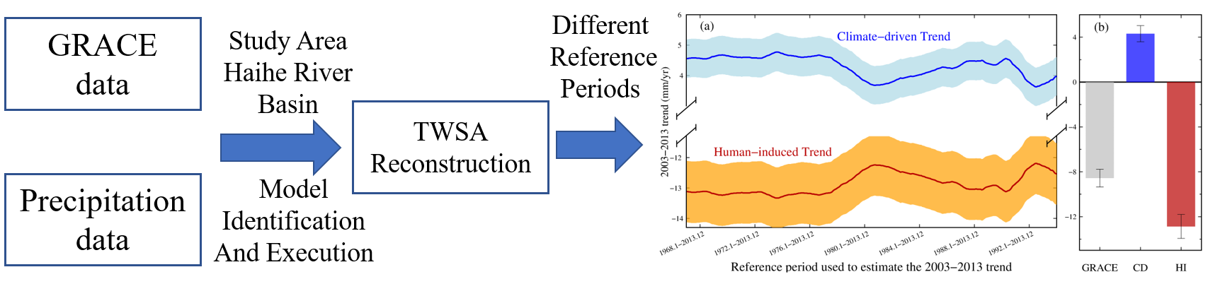
(a) Time series of climate-driven and human-induced TWSA trend of 2003–2013 relative to different reference periods. The light blue and orange shadows represent the uncertainties of these two trend time series. (b) TWSA trend budget in the HRB (gray bar: total TWSA trend from GRACE; blue bar: climate-driven TWSA trend; red bar: human-induced TWSA trend).
Figure 2.
(a) Time series of climate-driven and human-induced TWSA trend of 2003–2013 relative to different reference periods. The light blue and orange shadows represent the uncertainties of these two trend time series. (b) TWSA trend budget in the HRB (gray bar: total TWSA trend from GRACE; blue bar: climate-driven TWSA trend; red bar: human-induced TWSA trend).

Figure 3.
Interannual variations of (a) GRACE-derived, climate-driven and human-induced TWSA, and (b) their corresponding terrestrial water fluxes (TWF). The error bars show the uncertainties of annual TWSA and TWF.
Figure 3.
Interannual variations of (a) GRACE-derived, climate-driven and human-induced TWSA, and (b) their corresponding terrestrial water fluxes (TWF). The error bars show the uncertainties of annual TWSA and TWF.

Figure 4.
(a) Time series of climate-driven TWSA trend time series for 2003–2013 relative to different reference periods (blue curve, same as the blue curve in Figure 2a), and time series of annual precipitation trend for different reference periods (red curve). (b) Linear regression between annual precipitation trends during different reference periods and climate-driven trend estimates for 2003–2013. Noting that to are averaged to an annual trend value; other years are averaged in the same way in (b).

Table 1.
Climate-driven TWSA trends for the period of 2003–2013 corresponding to different reference periods (unit: mm/yr).
Table 1.
Climate-driven TWSA trends for the period of 2003–2013 corresponding to different reference periods (unit: mm/yr).
| Number i | Reference Period | Trend |
|---|---|---|
| 1 | 1967.01–2013.12 | 4.56 ± 0.63 () |
| 2 | 1967.02–2013.12 | 4.56 ± 0.63 () |
| … | … | … |
| 157 | 1980.01–2013.12 | 3.82 ± 0.63 () |
| … | … | … |
| 324 | 1993.12–2013.12 | 3.97 ± 0.63 () |
| Mean | 4.31 ± 0.72 () |
Table 2.
Estimates of GRACE-derived, climate-driven, and human-induced TWSA trends in the HRB from 2003 to 2013 based on different GRACE solutions and methods (unit: mm/yr).
Table 2.
Estimates of GRACE-derived, climate-driven, and human-induced TWSA trends in the HRB from 2003 to 2013 based on different GRACE solutions and methods (unit: mm/yr).
| GRACE-Derived TWSA Trend | Climate-Driven TWSA Trend | Human-Induced TWSA Trend | Description (GRACE Solution, Method) |
|---|---|---|---|
| −8.56 ± 0.79 | 4.31 ± 0.72 | −12.87 ± 1.07 | CSR-M, reconstruction |
| −9.86 ± 0.69 | 3.35 ± 0.66 | −13.21 ± 0.96 | GSFC-M, reconstruction |
| −14.20 ± 0.99 | 5.66 ± 0.95 | −19.86 ± 1.37 | JPL-M, reconstruction |
| −8.56 ± 0.79 | 1.09 ± 0.70 | −9.65 ± 1.06 | CSR-M, climate-driven TWSA from Noah |
| −8.56 ± 0.79 | 2.48 ± 0.69 | −11.04 ± 1.05 | CSR-M, climate-driven TWSA from CPC |
| −8.56 ± 0.79 | 2.49 ± 2.58 | −11.05 ± 2.46 | CSR-M, linear regression (Yi et al. 2016) |
| −8.56 ± 0.79 | 4.33 ± 0.63 | −12.89 ± 1.01 | CSR-M, reconstruction and linear regression |
| −8.56 ± 0.79 | 4.31 ± 0.71 | −12.87 ± 1.07 | CSR-M, reconstruction (detrended annual precipitation used) |
© 2019 by the authors. Licensee MDPI, Basel, Switzerland. This article is an open access article distributed under the terms and conditions of the Creative Commons Attribution (CC BY) license (http://creativecommons.org/licenses/by/4.0/).
Share and Cite
MDPI and ACS Style
Zhong, Y.; Feng, W.; Humphrey, V.; Zhong, M. Human-Induced and Climate-Driven Contributions to Water Storage Variations in the Haihe River Basin, China. Remote Sens. 2019, 11, 3050. https://0-doi-org.brum.beds.ac.uk/10.3390/rs11243050
AMA Style
Zhong Y, Feng W, Humphrey V, Zhong M. Human-Induced and Climate-Driven Contributions to Water Storage Variations in the Haihe River Basin, China. Remote Sensing. 2019; 11(24):3050. https://0-doi-org.brum.beds.ac.uk/10.3390/rs11243050
Chicago/Turabian StyleZhong, Yulong, Wei Feng, Vincent Humphrey, and Min Zhong. 2019. "Human-Induced and Climate-Driven Contributions to Water Storage Variations in the Haihe River Basin, China" Remote Sensing 11, no. 24: 3050. https://0-doi-org.brum.beds.ac.uk/10.3390/rs11243050
Note that from the first issue of 2016, this journal uses article numbers instead of page numbers. See further details here.