Remote Sensing Big Data Classification with High Performance Distributed Deep Learning

 , , , ,
Abstract
:
1. Introduction
2. Deep Learning
2.1. The ResNet
2.2. Distributed Frameworks
3. Experimental Setup
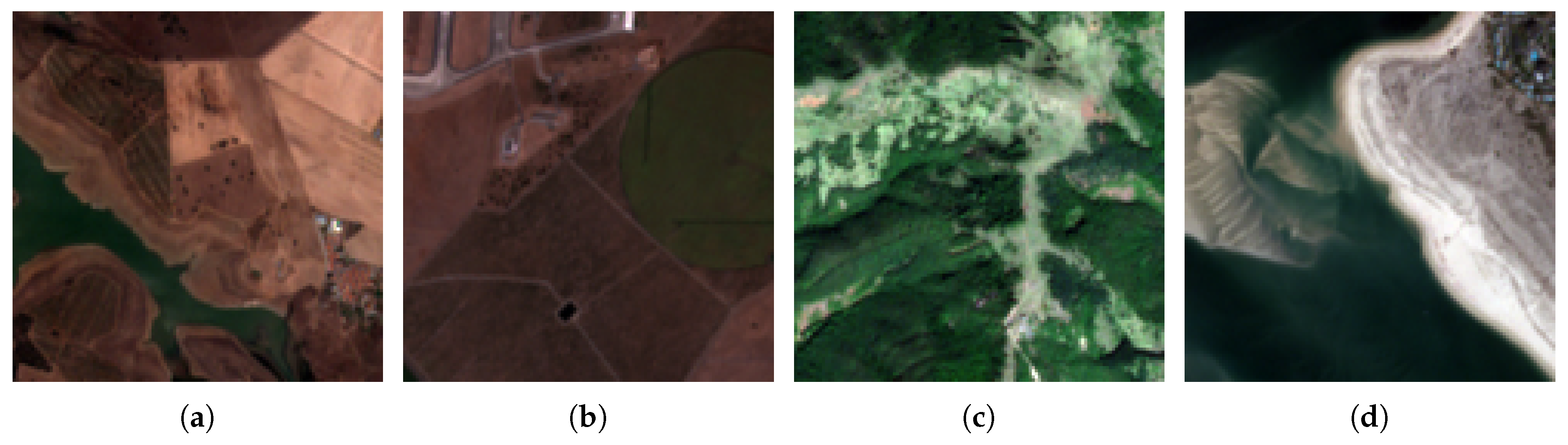
3.1. Data
3.2. Environment
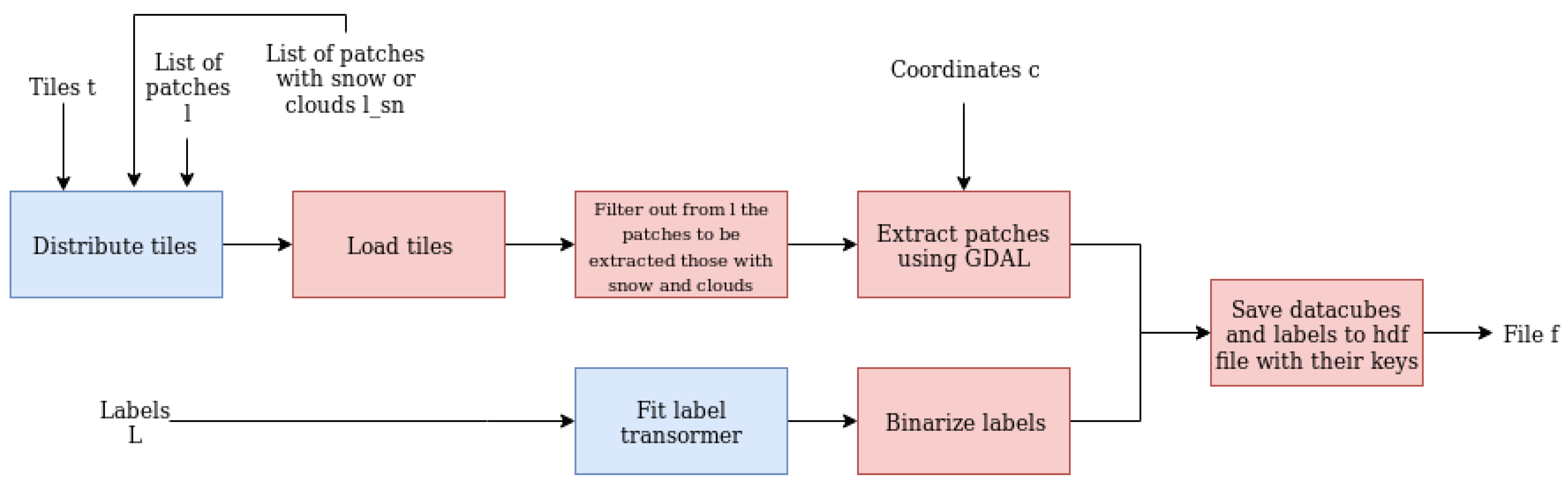
3.3. Preprocessing Pipeline
| Algorithm 1 Distribution of tiles |
Input: input parameters n number of CPUs and t tiles Output: matrix M with indices of tiles per processor
|
3.4. Multilabel Classification
3.5. Restricted RGB and Original Multispectral ResNet-50
4. Results
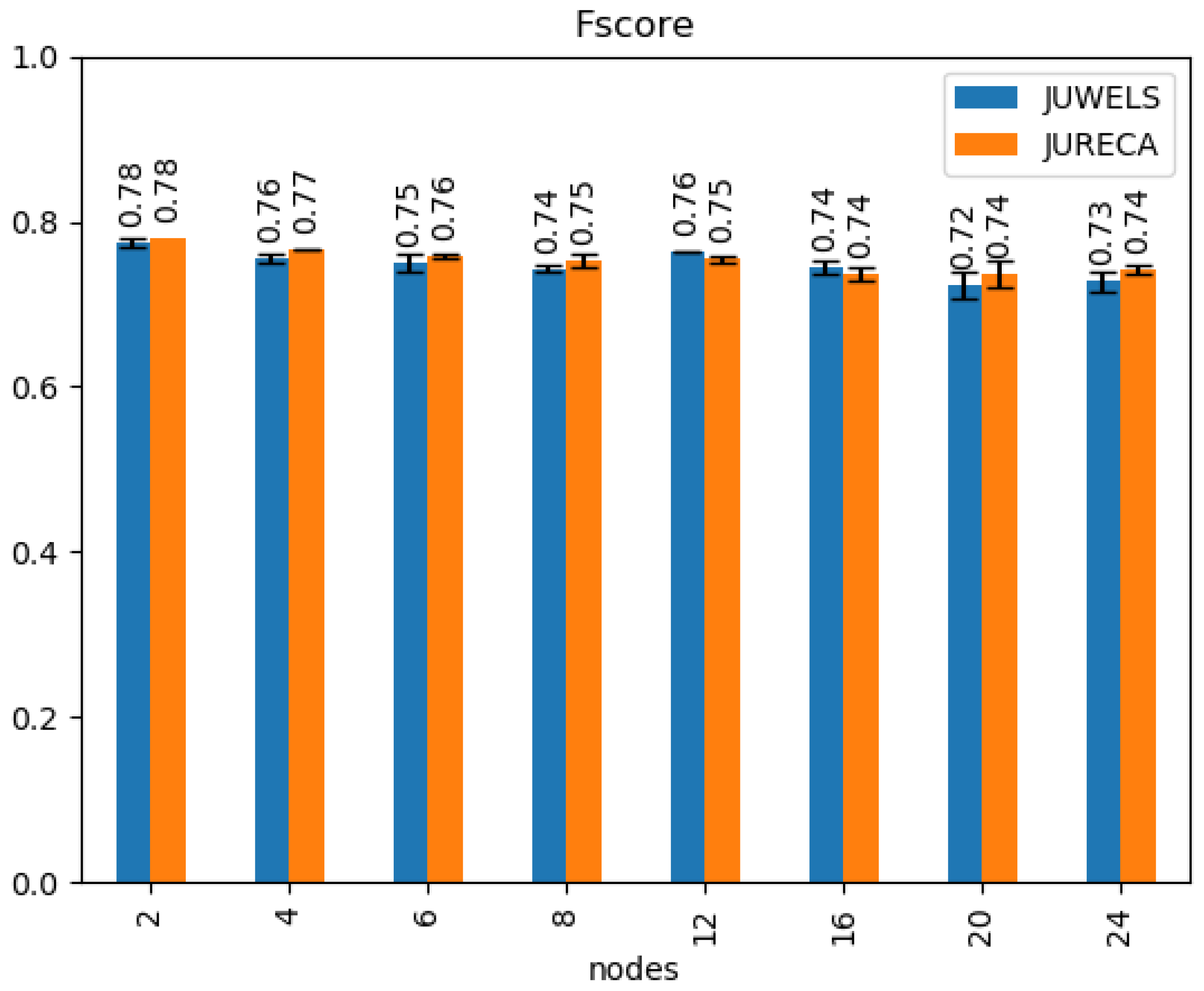
4.1. Classification
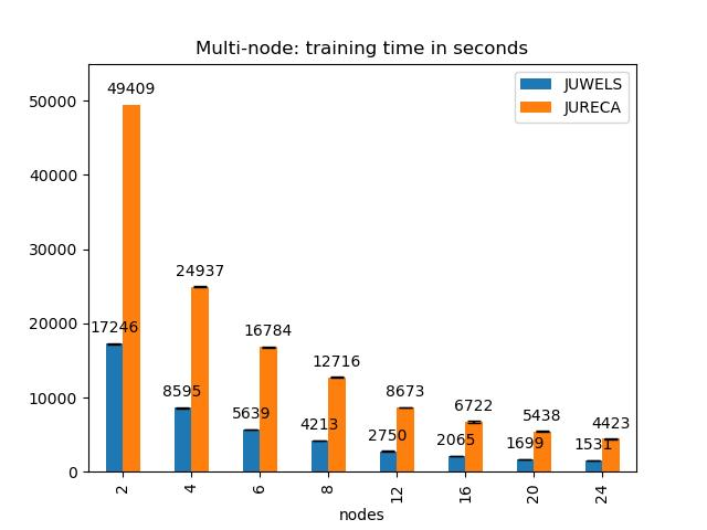
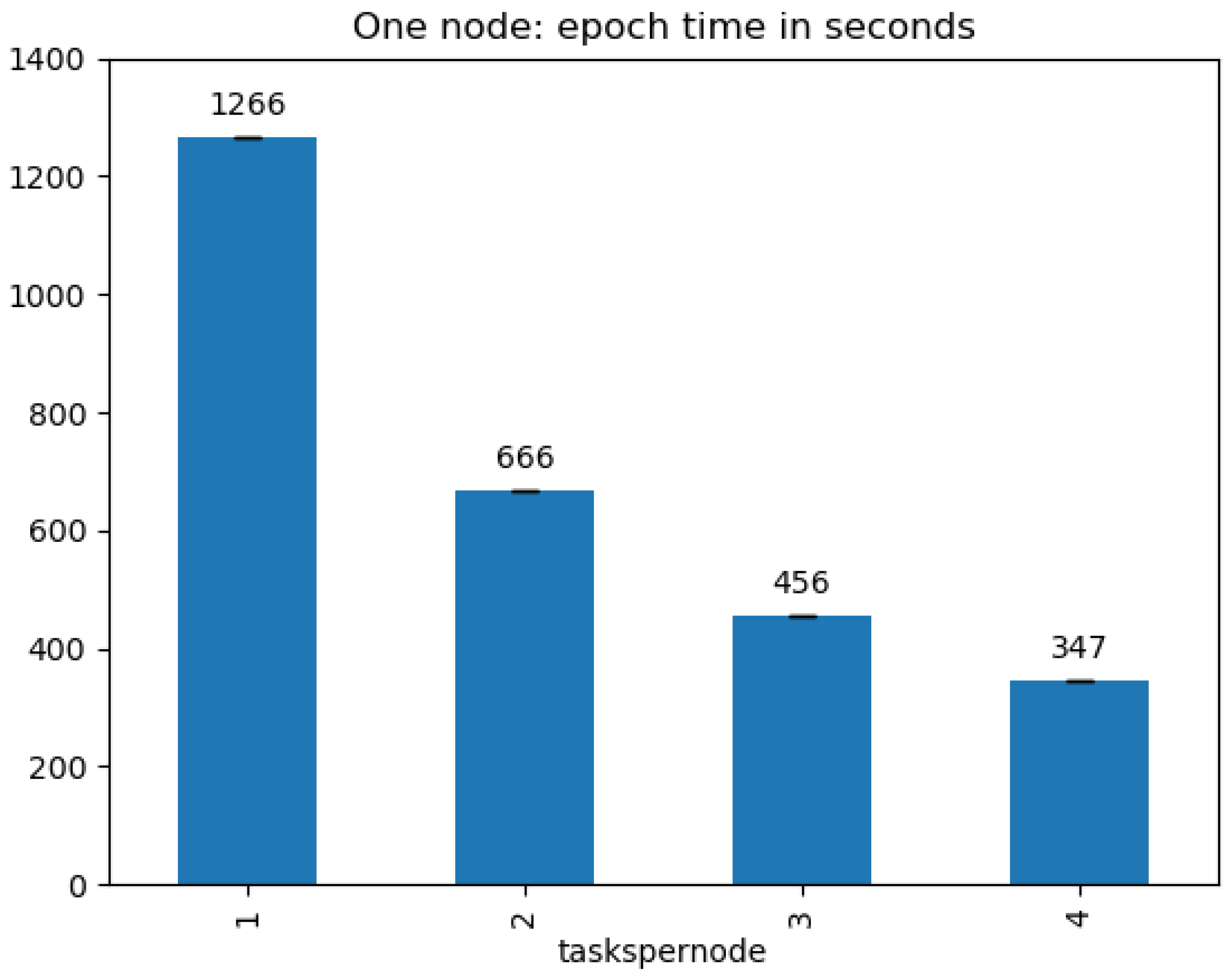
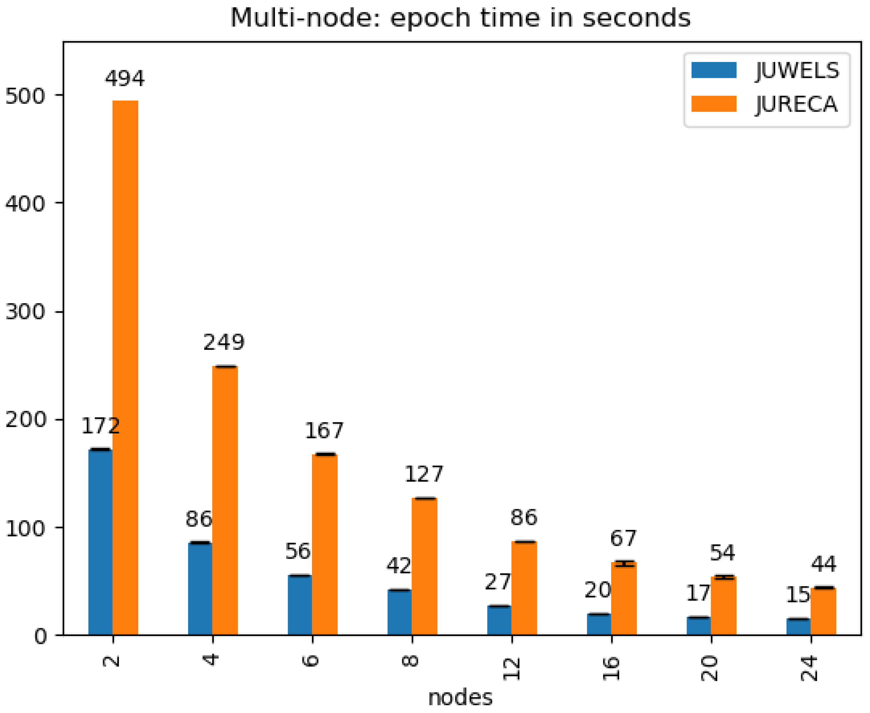
4.2. Processing Time
5. Discussion
6. Conclusions
Author Contributions
Funding
Conflicts of Interest
Abbreviations
| EO | Earth Observation |
| RS | Remote Sensing |
| DL | Deep Learning |
| ML | Machine Learning |
| HPC | High-Performance Computing |
| MPI | Message Passing Interface |
| CNN | Convolutional Neural Network |
| RNN | Recurrent Neural Network |
| GAN | Generative Adversarial Network |
| MS | Multispectral |
| ResNet | Residual Network |
| JUWELS | Jülich Wizard for European Leadership Science |
| JURECA | Jülich Research on Exascale Cluster Architectures |
| GPU | Graphics Processing Unit |
| CPU | Central Processing Unit |
| SGD | Stochastic Gradient Descent |
| CLS | CORINE Land Cover |
References
- Emery, W.; Camps, A. Basic Electromagnetic Concepts and Applications to Optical Sensors. In Introduction to Satellite Remote Sensing; Elsevier: Amsterdam, The Netherlands, 2017. [Google Scholar] [CrossRef]
- Wulder, M.A.; Masek, J.G.; Cohen, W.B.; Loveland, T.R.; Woodcock, C.E. Opening the archive: How free data has enabled the science and monitoring promise of Landsat. Remote. Sens. Environ. 2012. [Google Scholar] [CrossRef]
- Aschbacher, J. ESA’s earth observation strategy and Copernicus. In Satellite Earth Observations and Their Impact on Society and Policy; Springer: Singapore, 2017. [Google Scholar] [CrossRef] [Green Version]
- Ma, Y.; Wu, H.; Wang, L.; Huang, B.; Zomaya, A.; Jie, W. Remote sensing big data computing: Challenges and opportunities. Future Gener. Comput. Syst. 2015, 51, 47–60. [Google Scholar] [CrossRef]
- Chi, M.; Plaza, A.; Benediktsson, J.A.; Sun, Z.; Shen, J.; Zhu, Y. Big Data for Remote Sensing: Challenges and Opportunities. Proc. IEEE 2016. [Google Scholar] [CrossRef]
- Li, H.; Tao, C.; Wu, Z.; Chen, J.; Gong, J.; Deng, M. RSI-CB: Large Scale Remote. Sens. Image Classif. Benchmark Via Crowdsource Data. arXiv 2017, arXiv:1705.10450. [Google Scholar]
- Stoian, A.; Poulain, V.; Inglada, J.; Poughon, V.; Derksen, D. Land Cover Maps Production with High Resolution Satellite Image Time Series and Convolutional Neural Networks: Adaptations and Limits for Operational Systems. Remote. Sens. 2019, 11, 1986. [Google Scholar] [CrossRef] [Green Version]
- Ball, J.E.; Anderson, D.T.; Chan, C.S. A Comprehensive Survey of Deep Learning in Remote Sensing: Theories, Tools and Challenges for the Community. SPIE J. Appl. Remote. Sens. (JARS) Spec. Sect. Feature Deep. Learn. Remote. Sens. Appl. 2017, 11, 042609. [Google Scholar] [CrossRef] [Green Version]
- Zhu, X.X.; Tuia, D.; Mou, L.; Xia, G.S.; Zhang, L.; Xu, F.; Fraundorfer, F. Deep learning in remote sensing: A comprehensive review and list of resources. IEEE Geosci. Remote. Sens. Mag. 2017, 5, 8–36. [Google Scholar] [CrossRef] [Green Version]
- Ma, L.; Liu, Y.; Zhang, X.; Ye, Y.; Yin, G.; Johnson, B.A. Deep learning in remote sensing applications: A meta-analysis and review. ISPRS J. Photogramm. Remote. Sens. 2019, 152, 166–177. [Google Scholar] [CrossRef]
- Romero, A.; Gatta, C.; Camps-valls, G.; Member, S. Unsupervised Deep Feature Extraction for Remote Sensing Image Classification. IEEE Trans. Geosci. Remote. Sens. 2015, 54, 1–14. [Google Scholar] [CrossRef] [Green Version]
- Zhang, L.; Zhang, L.; Du, B. Deep Learning for Remote Sensing Data: A Technical Tutorial on the State of the Art. IEEE Geosci. Remote. Sens. Mag. 2016, 4, 22–40. [Google Scholar] [CrossRef]
- Ienco, D.; Gaetano, R.; Dupaquier, C.; Maurel, P. Land Cover Classification via Multitemporal Spatial Data by Deep Recurrent Neural Networks. IEEE Geosci. Remote. Sens. Lett. 2017. [Google Scholar] [CrossRef] [Green Version]
- Lin, D.; Fu, K.; Wang, Y.; Xu, G.; Sun, X. MARTA GANs: Unsupervised Representation Learning for Remote Sensing Image Classification. IEEE Geosci. Remote. Sens. Lett. 2017. [Google Scholar] [CrossRef] [Green Version]
- Cavallaro, G.; Falco, N.; Dalla Mura, M.; Benediktsson, J.A. Automatic Attribute Profiles. IEEE Trans. Image Process. 2017. [Google Scholar] [CrossRef] [PubMed] [Green Version]
- Sumbul, G.; Charfuelan, M.; Demir, B.; Markl, V. Bigearthnet: Large-Scale Benchmark Arch. Remote. Sens. Image Underst. arXiv 2019, arXiv:1902.06148. [Google Scholar]
- Plaza, A.; Valencia, D.; Plaza, J.; Martinez, P. Commodity cluster-based parallel processing of hyperspectral imagery. J. Parallel Distrib. Comput. 2006. [Google Scholar] [CrossRef]
- Gorgan, D.; Bacu, V.; Stefanut, T.; Rodila, D.; Mihon, D. Grid based satellite image processing platform for Earth Observation application development. In Proceedings of the 5th IEEE International Workshop on Intelligent Data Acquisition and Advanced Computing Systems: Technology and Applications, IDAACS’2009, Rende, Italy, 21–23 September 2009. [Google Scholar] [CrossRef]
- Foster, I.; Zhao, Y.; Raicu, I.; Lu, S. Cloud computing and grid computing 360-degree compared. In Proceedings of the Grid Comput. Environ. Workshop 2008 (GCE ’08), Austin, TX, USA, 12–16 November 2008; pp. 1–10. [Google Scholar] [CrossRef] [Green Version]
- McKinney, R.; Pallipuram, V.K.; Vargas, R.; Taufer, M. From HPC performance to climate modeling: Transforming methods for HPC predictions into models of extreme climate conditions. In Proceedings of the 11th IEEE International Conference on eScience, eScience 2015, Munich, Germany, 31 August–4 September 2015. [Google Scholar] [CrossRef]
- Yang, Y.; Newsam, S. Bag-of-visual-words and spatial extensions for land-use classification. In Proceedings of the ACM International Symposium on Advances in Geographic Information Systems, San Jose, CA, USA, 2–5 November 2010. [Google Scholar] [CrossRef]
- Li, J.; Bioucas-Dias, J.M.; Plaza, A. Spectral-spatial classification of hyperspectral data using loopy belief propagation and active learning. IEEE Trans. Geosci. Remote. Sens. 2013. [Google Scholar] [CrossRef]
- Zou, Q.; Ni, L.; Zhang, T.; Wang, Q. Deep Learning Based Feature Selection for Remote Sensing Scene Classification. IEEE Geosci. Remote. Sens. Lett. 2015. [Google Scholar] [CrossRef]
- Basu, S.; Ganguly, S.; Mukhopadhyay, S.; DiBiano, R.; Karki, M.; Nemani, R. DeepSat—A learning framework for satellite imagery. In Proceedings of the ACM International Symposium on Advances in Geographic Information Systems, Seattle, WD, USA, 3–6 November 2015. [Google Scholar] [CrossRef]
- Zhao, B.; Zhong, Y.; Xia, G.S.; Zhang, L. Dirichlet-derived multiple topic scene classification model for high spatial resolution remote sensing imagery. IEEE Trans. Geosci. Remote. Sens. 2016. [Google Scholar] [CrossRef]
- Zhao, L.; Tang, P.; Huo, L. Feature significance-based multibag-of-visual-words model for remote sensing image scene classification. J. Appl. Remote. Sens. 2016, 10, 1–21. [Google Scholar] [CrossRef]
- Penatti, O.A.; Nogueira, K.; Dos Santos, J.A. Do deep features generalize from everyday objects to remote sensing and aerial scenes domains? In Proceedings of the IEEE Computer Society Conference on Computer Vision and Pattern Recognition Workshops, Boston, MA, USA, 7–12 June 2015. [Google Scholar] [CrossRef] [Green Version]
- Cheng, G.; Han, J.; Lu, X. Remote. Sens. Image Scene Classif. Benchmark State Art. Proc. IEEE 2017, 1865–1883. [Google Scholar] [CrossRef] [Green Version]
- Xia, G.S.; Hu, J.; Hu, F.; Shi, B.; Bai, X.; Zhong, Y.; Zhang, L.; Lu, X. AID: A benchmark data set for performance evaluation of aerial scene classification. IEEE Trans. Geosci. Remote. Sens. 2017. [Google Scholar] [CrossRef] [Green Version]
- Helber, P.; Bischke, B.; Dengel, A.; Borth, D. EuroSAT: A Novel Dataset and Deep Learning Benchmark for Land Use and Land Cover Classification. Comput. Res. Repos. 2017. [Google Scholar] [CrossRef]
- Zhou, W.; Newsam, S.; Li, C.; Shao, Z. PatternNet: A benchmark dataset for performance evaluation of remote sensing image retrieval. ISPRS J. Photogramm. Remote. Sens. 2018. [Google Scholar] [CrossRef] [Green Version]
- He, K.; Zhang, X.; Ren, S.; Sun, J. Deep residual learning for image recognition. In Proceedings of the IEEE Computer Society Conference on Computer Vision and Pattern Recognition, Vegas, NV, USA, 27–30 June 2016. [Google Scholar] [CrossRef] [Green Version]
- He, K.; Zhang, X.; Ren, S.; Sun, J. Identity mappings in deep residual networks. In Proceedings of the European Conference on Computer Vision, Amsterdam, The Netherlands, 11–14 October 2016; pp. 630–645. [Google Scholar]
- Russakovsky, O.; Deng, J.; Su, H.; Krause, J.; Satheesh, S.; Ma, S.; Huang, Z.; Karpathy, A.; Khosla, A.; Bernstein, M.; et al. ImageNet large scale visual recognition challenge. Int. J. Comput. Vis. 2015, 115, 211–252. [Google Scholar] [CrossRef] [Green Version]
- Krizhevsky, A.; Sutskever, I.; Hinton, G.E. Imagenet classification with deep convolutional neural networks. In Advances in Neural Information Processing Systems, NIPS Proceedings of the 25th International Conference on Neural Information Processing Systems, Lake Tahoe, Nevada, NV, USA, 3–6 December 2012; The MIT Press: London, UK, 2012; pp. 1097–1105. [Google Scholar]
- Simonyan, K.; Zisserman, A. Very deep convolutional networks for large-scale image recognition. arXiv 2014, arXiv:1409.1556. [Google Scholar]
- Szegedy, C.; Wei, L.; Jia, Y.; Sermanet, P.; Reed, S.; Anguelov, D.; Erhan, D.; Vanhoucke, V.; Rabinovich, A. Going deeper with convolutions. In Proceedings of the IEEE Conf. Computer Vision and Pattern Recognition (CVPR), Boston, MA, USA, 7–12 June 2015; pp. 1–9. [Google Scholar] [CrossRef] [Green Version]
- Deng, J.; Dong, W.; Socher, R.; Li, L.; Li, K.; Li, F.-F. ImageNet: A large-scale hierarchical image database. In Proceedings of the IEEE Conf. Computer Vision and Pattern Recognition, Miami, FL, USA, 20–25 June 2009; pp. 248–255. [Google Scholar] [CrossRef] [Green Version]
- Donahue, J.; Jia, Y.; Vinyals, O.; Hoffman, J.; Zhang, N.; Tzeng, E.; Darrell, T. Decaf: A deep convolutional activation feature for generic visual recognition. In Proceedings of the International Conference on Machine Learning, Bejing, China, 22–24 June 2014; pp. 647–655. [Google Scholar]
- Razavian, A.S.; Azizpour, H.; Sullivan, J.; Carlsson, S. CNN Features Off-the-Shelf: An Astounding Baseline for Recognition. In Proceedings of the IEEE Conf. Computer Vision and Pattern Recognition Workshops, Columbus, OH, USA, 23–28 June 2014; pp. 512–519. [Google Scholar] [CrossRef] [Green Version]
- Kornblith, S.; Shlens, J.; Le, Q.V. Do better imagenet models transfer better? In Proceedings of the IEEE Conference on Computer Vision and Pattern Recognition, Beach, CA, USA, 16–20 Junary 2019; pp. 2661–2671. [Google Scholar]
- Mayer, R.; Jacobsen, H.A. Scalable Deep Learning on Distributed Infrastructures: Challenges, Techniques and Tools. arXiv 2019, arXiv:1903.11314. [Google Scholar]
- You, Y.; Zhang, Z.; Hsieh, C.; Demmel, J.; Keutzer, K. Fast Deep Neural Network Training on Distributed Systems and Cloud TPUs. IEEE Trans. Parallel Distrib. Syst. 2019. [Google Scholar] [CrossRef]
- Ying, C.; Kumar, S.; Chen, D.; Wang, T.; Cheng, Y. Image classification at supercomputer scale. arXiv 2018, arXiv:1811.06992. [Google Scholar]
- Yamazaki, M.; Kasagi, A.; Tabuchi, A.; Honda, T.; Miwa, M.; Fukumoto, N.; Tabaru, T.; Ike, A.; Nakashima, K. Yet Another Accelerated SGD: ResNet-50 Training on ImageNet in 74.7 seconds. arXiv 2019, arXiv:1903.12650. [Google Scholar]
- Sergeev, A.; Balso, M.D. Horovod: Fast and easy distributed deep learning in TensorFlow. arXiv 2018, arXiv:1802.05799. [Google Scholar]
- Gibiansky, A. Bringing HPC Techniques to Deep Learning. Available online: http://andrew.gibiansky.com/blog/machine-learning/baidu-allreduce/ (accessed on 1 April 2019).
- NVIDIA Collective Communications Library (NCCL). Available online: https://developer.nvidia.com/nccl (accessed on 15 October 2019).
- TensorFlow Distributed Strategy Documentation. Available online: https://www.tensorflow.org/guide/distributed_training (accessed on 1 April 2019).
- Goyal, P.; Dollár, P.; Girshick, R.; Noordhuis, P.; Wesolowski, L.; Kyrola, A.; Tulloch, A.; Jia, Y.; He, K. Accurate, Large Minibatch SGD: Training ImageNet in 1 Hour. arXiv 2017, arXiv:1706.02677. [Google Scholar]
- You, Y.; Gitman, I.; Ginsburg, B. Scaling sgd batch size to 32k for imagenet training. arXiv 2017, arXiv:1708.03888. [Google Scholar]
- Sentinel2 B10: High Atmospheric Absorption Band. Available online: https://sentinel.esa.int/web/sentinel/technical-guides/sentinel-2-msi/level-1c/cloud-masks (accessed on 15 May 2019).
- Scripts to Remove Cloudy and Snowy Patches Provided by BigEarthNet Archive Creators from the Remote Sensing Image Analysis (RSiM) Group at the TU Berlin. Available online: http://bigearth.net/ (accessed on 1 April 2019).
- Jülich Supercomputing Centre. JUWELS: Modular Tier-0/1 Supercomputer at the Jülich Supercomputing Centre. J. Large-Scale Res. Facil. 2019, 5. [Google Scholar] [CrossRef] [Green Version]
- Jülich Supercomputing Centre. JURECA: Modular supercomputer at Jülich Supercomputing Centre. J. Large-Scale Res. Facil. 2018, 4. [Google Scholar] [CrossRef] [Green Version]
- Lanaras, C.; Bioucas-Dias, J.; Galliani, S.; Baltsavias, E.; Schindler, K. Super-resolution of Sentinel-2 images: Learning a globally applicable deep neural network. ISPRS J. Photogramm. Remote. Sens. 2018. [Google Scholar] [CrossRef] [Green Version]
- GDAL/OGR contributors. GDAL/OGR Geospatial Data Abstraction Software Library; Open Source Geospatial Foundation: Chicago, IL, USA, 2019. [Google Scholar]
- The HDF Group. Hierarchical Data Format, Version 5, 1997-NNNN. Available online: http://www.hdfgroup.org/HDF5/ (accessed on 1 April 2019).
- Chaudhuri, B.; Demir, B.; Chaudhuri, S.; Bruzzone, L. Multilabel Remote Sensing Image Retrieval Using a Semisupervised Graph-Theoretic Method. IEEE Trans. Geosci. Remote. Sens. 2018, 56, 1144–1158. [Google Scholar] [CrossRef]
- Read, J.; Pfahringer, B.; Holmes, G.; Frank, E. Classifier Chains for Multi-label Classification. In Machine Learning and Knowledge Discovery in Databases; Buntine, W., Grobelnik, M., Mladenić, D., Shawe-Taylor, J., Eds.; Springer: Berlin/Heidelberg, Germany, 2009; pp. 254–269. [Google Scholar]
- Zhang, H.; Cisse, M.; Dauphin, Y.N.; Lopez-Paz, D. mixup: Beyond Empirical Risk Minimization. arXiv 2017, arXiv:1710.09412. [Google Scholar]
- Sutskever, I.; Martens, J.; Dahl, G.; Hinton, G. On the importance of initialization and momentum in deep learning. In Proceedings of the 30th International Conference on Machine Learning, ICML 2013, Atlanta, GA, USA, 16–21 June 2013. [Google Scholar]
- Bengio, Y. Practical recommendations for gradient-based training of deep architectures. Lect. Notes Comput. Sci. (Incl. Subser. Lect. Notes Artif. Intell. Lect. Notes Bioinform.) 2012. [Google Scholar] [CrossRef]
- Johnson, J.M.; Khoshgoftaar, T.M. Survey on deep learning with class imbalance. J. Big Data 2019. [Google Scholar] [CrossRef]
- Buda, M.; Maki, A.; Mazurowski, M.A. A systematic study of the class imbalance problem in convolutional neural networks. Neural Netw. 2018. [Google Scholar] [CrossRef] [Green Version]
- Parikh, N. Accurate, Large Minibatch SGD: Training ImageNet in 1 Hour. Found. Trends Optim. 2014. [Google Scholar] [CrossRef]


| Datasets | Image Type | Image Per Class | Scene Classes | Annotation Type | Total Images | Spatial Resolution (m) | Image Sizes | Year | Ref. |
|---|---|---|---|---|---|---|---|---|---|
| UC Merced | Aerial RGB | 100 | 21 | Single/Multi label | 2100 | 0.3 | 256 × 256 | 2010 | [21] |
| WHU-RS19 | Aerial RGB | ∼50 | 19 | Single label | 1005 | up to 0.5 | 600 × 600 | 2012 | [22] |
| RSSCN7 | Aerial RGB | 400 | 7 | Single label | 2800 | – | 400 × 400 | 2015 | [23] |
| SAT-6 | Aerial MS | – | 6 | Single label | 405,000 | 1 | 28 × 28 | 2015 | [24] |
| SIRI-WHU | Aerial RGB | 200 | 12 | Single label | 2400 | 2 | 200 × 200 | 2016 | [25] |
| RSC11 | Aerial RGB | 100 | 11 | Single label | 1323 | 0.2 | 512 × 512 | 2016 | [26] |
| Brazilian Coffee | Satellite MS | 1438 | 2 | Single label | 2876 | – | 64 × 64 | 2016 | [27] |
| RESISC45 | Aerial RGB | 700 | 45 | Single label | 31500 | 30 to 0.2 | 256 × 256 | 2016 | [28] |
| AID | Aerial RGB | ∼300 | 30 | Single label | 10,000 | 0.6 | 600 × 600 | 2016 | [29] |
| EuroSAT | Satellite MS | ∼2500 | 10 | Single label | 27,000 | 10 | 64 × 64 | 2017 | [30] |
| RSI-CB128 | Aerial RGB | ∼800 | 45 | Single label | 36,000 | 0.3 to 3 | 128 × 128 | 2017 | [6] |
| RSI-CB256 | Aerial RGB | ∼690 | 35 | Single label | 24,000 | 0.3 to 3 | 256 × 256 | 2017 | [6] |
| PatternNet | Aerial RGB | ∼800 | 38 | Single label | 30,400 | 0.062∼4.693 | 256 × 256 | 2017 | [31] |
| 120 × 120 | |||||||||
| BigEarthNet | Satellite MS | 328 to 217,119 | 43 | Multi label | 590,326 | 10,20,60 | 60 × 60 | 2018 | [16] |
| 20 × 20 |
| P | R | F1 | ||
|---|---|---|---|---|
| RGB | 0.82 | 0.71 | 0.77 | |
| multispectral | 0.83 | 0.75 | 0.79 |
| Support | F1 (Multispectral) | F1 (RGB) | |
|---|---|---|---|
| Agro-forestry areas | 5611 | 0.803621 | 0.795872 |
| Airports | 157 | 0.300518 | 0.374384 |
| Annual crops associated with permanent crops | 1275 | 0.457738 | 0.442318 |
| Bare rock | 511 | 0.604819 | 0.620192 |
| Beaches, dunes, sands | 319 | 0.695810 | 0.608964 |
| Broad-leaved forest | 28,090 | 0.791465 | 0.771761 |
| Burnt areas | 66 | 0.029851 | 0 |
| Coastal lagoons | 287 | 0.884758 | 0.880294 |
| Complex cultivation patterns | 21,142 | 0.722448 | 0.698238 |
| Coniferous forest | 33,583 | 0.874152 | 0.866716 |
| Construction sites | 244 | 0.234482 | 0.213058 |
| Continuous urban fabric | 1975 | 0.784672 | 0.517737 |
| Discontinuous urban fabric | 13,338 | 0.780262 | 0.722825 |
| Dump sites | 181 | 0.287037 | 0.268518 |
| Estuaries | 197 | 0.699088 | 0.585034 |
| Fruit trees and berry plantations | 875 | 0.452648 | 0.417887 |
| Green urban areas | 338 | 0.387750 | 0.369477 |
| Industrial or commercial units | 2417 | 0.552506 | 0.556856 |
| Inland marshes | 1142 | 0.408505 | 0.364675 |
| Intertidal flats | 216 | 0.635097 | 0.584126 |
| Land principally occupied by agriculture | 26,447 | 0.686677 | 0.667633 |
| Mineral extraction sites | 835 | 0.507598 | 0.490980 |
| Mixed forest | 35,975 | 0.834221 | 0.797793 |
| Moors and heathland | 1060 | 0.561134 | 0.430953 |
| Natural grassland | 2273 | 0.569581 | 0.512231 |
| Non-irrigated arable land | 36,562 | 0.865387 | 0.839924 |
| Olive groves | 2372 | 0.621071 | 0.541914 |
| Pastures | 20,770 | 0.780565 | 0.771802 |
| Peatbogs | 3411 | 0.535477 | 0.690319 |
| Permanently irrigated land | 2505 | 0.675662 | 0.643835 |
| Port areas | 93 | 0.503597 | 0.522388 |
| Rice fields | 709 | 0.669542 | 0.604770 |
| Road and rail networks and associated land | 671 | 0.300785 | 0.268623 |
| Salines | 75 | 0.608000 | 0.517857 |
| Salt marshes | 264 | 0.568578 | 0.532299 |
| Sclerophyllous vegetation | 2114 | 0.762123 | 0.671300 |
| Sea and ocean | 13,964 | 0.909013 | 0.979917 |
| Sparsely vegetated areas | 261 | 0.483460 | 0.380681 |
| Sport and leisure facilities | 996 | 0.367029 | 0.406827 |
| Transitional woodland/shrub | 29,671 | 0.664189 | 0.639412 |
| Vineyards | 1821 | 0.564012 | 0.545454 |
| Water bodies | 11,545 | 0.858107 | 0.823858 |
| Water courses | 1914 | 0.803948 | 0.737060 |
© 2019 by the authors. Licensee MDPI, Basel, Switzerland. This article is an open access article distributed under the terms and conditions of the Creative Commons Attribution (CC BY) license (http://creativecommons.org/licenses/by/4.0/).
Share and Cite
Sedona, R.; Cavallaro, G.; Jitsev, J.; Strube, A.; Riedel, M.; Benediktsson, J.A. Remote Sensing Big Data Classification with High Performance Distributed Deep Learning. Remote Sens. 2019, 11, 3056. https://0-doi-org.brum.beds.ac.uk/10.3390/rs11243056
Sedona R, Cavallaro G, Jitsev J, Strube A, Riedel M, Benediktsson JA. Remote Sensing Big Data Classification with High Performance Distributed Deep Learning. Remote Sensing. 2019; 11(24):3056. https://0-doi-org.brum.beds.ac.uk/10.3390/rs11243056
Chicago/Turabian StyleSedona, Rocco, Gabriele Cavallaro, Jenia Jitsev, Alexandre Strube, Morris Riedel, and Jón Atli Benediktsson. 2019. "Remote Sensing Big Data Classification with High Performance Distributed Deep Learning" Remote Sensing 11, no. 24: 3056. https://0-doi-org.brum.beds.ac.uk/10.3390/rs11243056