Combining Optical, Fluorescence, Thermal Satellite, and Environmental Data to Predict County-Level Maize Yield in China Using Machine Learning Approaches

Abstract

Maize is an extremely important grain crop, and the demand has increased sharply throughout the world. China contributes nearly one-fifth of the total production alone with its decreasing arable land. Timely and accurate prediction of maize yield in China is critical for ensuring global food security. Previous studies primarily used either visible or near-infrared (NIR) based vegetation indices (VIs), or climate data, or both to predict crop yield. However, other satellite data from different spectral bands have been underutilized, which contain unique information on crop growth and yield. In addition, although a joint application of multi-source data significantly improves crop yield prediction, the combinations of input variables that could achieve the best results have not been well investigated. Here we integrated optical, fluorescence, thermal satellite, and environmental data to predict county-level maize yield across four agro-ecological zones (AEZs) in China using a regression-based method (LASSO), two machine learning (ML) methods (RF and XGBoost), and deep learning (DL) network (LSTM). The results showed that combining multi-source data explained more than 75% of yield variation. Satellite data at the silking stage contributed more information than other variables, and solar-induced chlorophyll fluorescence (SIF) had an almost equivalent performance with the enhanced vegetation index (EVI) largely due to the low signal to noise ratio and coarse spatial resolution. The extremely high temperature and vapor pressure deficit during the reproductive period were the most important climate variables affecting maize production in China. Soil properties and management factors contained extra information on crop growth conditions that cannot be fully captured by satellite and climate data. We found that ML and DL approaches definitely outperformed regression-based methods, and ML had more computational efficiency and easier generalizations relative to DL. Our study is an important effort to combine multi-source remote sensed and environmental data for large-scale yield prediction. The proposed methodology provides a paradigm for other crop yield predictions and in other regions.

1. Introduction

Maize is a staple food for more than 4.5 billion people, and the demand is expected to double by 2050 [1,2,3]. China is the second-largest producer and consumer of maize, and the country contributes to 21% of the global production with less than 9% of maize planting areas [4]. Therefore, timely and accurate prediction of maize yield in China is vital for both regional and global food security.

Traditional crop yield estimation primarily relies on crop models and statistical regression [5,6,7]. Crop models could reproduce the key processes of plant growth and development in detail and can run on multiple scales [8,9]. However, they are often computationally intensive and require fine soil and daily weather data, which prevent their large-scale application [10,11]. In contrast, statistical-based methods provide a simpler alternative for yield prediction, but such empirical models are typically localized and unable to extend to other areas [7,12]. Machine learning (ML) is an immediate successor of the statistical method, which adopts important weights rather than the likelihood or probability of any forecasting information [13]. Therefore, ML is more effective for noisy data and is able to interpret nonlinear relationships. ML has been increasingly and extensively used for crop classification and yield estimation [14,15]. For instance, Hunt et al. [16] trained an RF model with high-resolution sentinel-2 images and mapped within-field wheat yield at 10 m resolution in the UK. Cai et al. [17] accurately predicted county-level wheat yield in Australia using three ML methods (RF, SVR, and NN), and confirmed that their performances were much better than the traditional regression model. Deep learning (DL) is an advanced approach for performing ML tasks [18], which has substantiated its advantages in many fields, such as image capturing and speech recognition [18,19,20,21]. However, there are still limited studies that applied DL to crop yield prediction [18]. In addition, whether emerging data-driven approaches outperform the regression-based method has not been well investigated.

ML and DL methods require multiple factors relating to crop growth and development, for example, satellite observations, climate variables, and soil properties, for capturing yield variability [22,23,24,25]. Remote sensing provides data on a large spatial context and can directly monitor crop status through various spectra, such as optical, thermal, and microwave wavelengths. Previous studies mostly used visible and near-infrared (NIR) (optical) based vegetation indices (VIs), like the normalized difference vegetation index (NDVI) and enhanced vegetation index (EVI) to predict crop yield [5,25,26]. The two VIs are similar, but the EVI is less affected by higher canopy leaf area index (LAI) [26]. However, VIs mainly reflect the leaf structure and greenness of vegetation, other than environmental stress on crop growth [6,12,17]. Solar-induced chlorophyll fluorescence (SIF), a newly detected signal in the NIR (650–800 nm), contains information about the physiological, biochemical, and the fraction of absorbed photosynthetically active radiation (fPAR) [27,28]. SIF is a proxy of photosynthesis and responds to crop stress more sensitively than VIs [29,30]. However, very limited studies so far have explored whether SIF outperforms EVI in estimating crop yield at larger scales.

Climate variables, such as temperature- and water-related variables, reflect crop stress from growth conditions, which cannot capture by satellite data. Land-surface temperature (LST) from thermal bands is a critical variable for detecting crop stress from leaf canopy temperatures [31,32,33]. Heft-Neal et al. [34] substituted ground-observed maximum air temperature (Tair) with LST to estimate maize yield and achieved a better result in Africa. Pede et al. [12] also reported that LST had improved maize yield predictions and could accurately forecast them several months in advance relative to Tair in the US. However, the majority of agriculture studies have not yet utilized LST. To our knowledge, there is still no study focusing on remotely sensed LST for crop yield prediction on large scales in China to date.

Previous studies have confirmed that water supply significantly affects maize production, especially in extremely hot periods [35,36,37,38]. However, precipitation may be an inadequate indicator of water availability. The actual available water for crops highly depends on soil moisture, which relates to several soil characteristics, including soil water holding capacity, soil quality and type, and rooting depth [39,40]. Furthermore, soil property varies greatly across the whole of China, resulting in a highly variable growing condition for crops. Additionally, soil property is considered as one of the important factors that lead to a large yield gap in the Chinese Maize Belt [41,42]. Hence, large-scale crop yield estimation should integrate soil features with climate variables to better capture the variation of yield [14,17]. Previous studies have also reported that a joint application of multi-source data could improve crop yield prediction [12,17,23,29]. However, which combinations of input variables could achieve the best results is unclear.

Here, we integrated optical, fluorescence, thermal satellite data, and environmental variables (climate variables, soil properties, and irrigation ratio) to predict the county-level maize yield in China from 2001 to 2015 by applying four methods: least absolute shrinkage and selection operator (LASSO), random forest (RF), extreme gradient boosting (XGBoost) and long short-term memory (LSTM). We aimed to answer the following questions: (1) Does SIF, a proxy of plant photosynthesis, outperform EVI in predicting maize yield at regional scales? (2) How do ML and DL perform when compared with traditional linear regression for estimating crop yield? (3) Which combinations of input variables could achieve the best results?

2. Materials and Methods

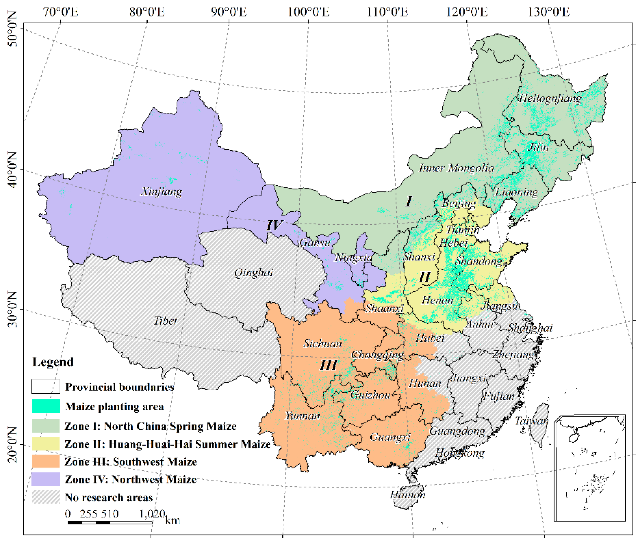
2.1. Study Area

The main maize-growing regions are divided into four agro-ecological zones (AEZs) according to the cultivar characteristics, management practices, and geographical environments (Figure 1). The typical growth cycles of maize in each AEZ are shown in Figure S1.

Zone I (North China spring maize) has a continental monsoon climate, rich and deep soil, and a mean temperature of 8.6 °C. The total annual precipitation ranges from 400 to 800 mm. The maize and wheat double rotation is the dominant cropping system and contributes to 39% of the national total maize production.

Zone II (Huang-Huai-Hai summer maize) has a semi-humid monsoon climate, alluvial soil, and a mean temperature ranging from 8–15 °C. The annual precipitation is very uneven, ranging from 400 mm in the northwest to 2000 mm in the southeast. The main cropping system is the winter wheat and summer maize rotation, which produces one-third of maize.

Zone III (Southwest maize) has a subtropical monsoon humid climate, lime purple soil, and a mean temperature of approximate 24 °C. The annual precipitation exceeds 990 mm. The prevailing planting pattern is an intensive triple-cropping system that includes rice, maize, and wheat. The maize production accounts for 13.4% of the total yield.

Zone IV (Northwest maize) has a monsoon climate of medium latitudes, Loess, and a mean temperature of approximately 9.5 °C. The annual precipitation decreases from 400 mm in the east to less than 50 mm in the west. The main planted crops are winter wheat and spring maize. The maize production contributes to approximately 10% of the national yield.

2.2. Data

We collected multi-source data with various spatial and temporal resolutions, including annual maize planting areas and county-level yield, satellite data, and environmental factors (i.e., climate variables, soil properties, and irrigation ratio). An overview of the data was presented in Table S1. Here, we first resampled the gridded data into 1 km and monthly time steps and then aggregated all input data to a mean for each county after being masked by maize planting areas. All these processes were implemented on the GEE (Google Earth Engine) platform.

2.2.1. Maize Yield and Planting Area

County-level maize yield (kg/ha) from 2001 to 2015 was collected from the ‘Agricultural Statistical Yearbook’ compiled by the Ministry of Agriculture of China. Annual maize planting areas were based on previous work [43] in which maize-cropping areas were identified at a resolution of 1 km in China from 2000 to 2015 (https://0-doi-org.brum.beds.ac.uk/10.6084/m9.figshare.8313530). The counties were selected in the light of having yield data and more than six planting grids for at least 8 years out of a 15-year study period. Finally, 1198 counties were selected, covering approximately 50% of cropping areas in China.

2.2.2. Satellite Data

Monthly maximum values of two vegetation metrics (EVI and SIF) in the growing season were used to reflect aboveground vegetation dynamics associated with biomass and photosynthesis. We used the latest version (Collection 6) MODIS EVI with 1 km and 16-day resolution during the period of 2001–2015 from the MOD13A2 product, which obtained from the GEE platform (https://0-doi-org.brum.beds.ac.uk/10.5067/MODIS/MOD13A2.006). SIF data was a global spatially contiguous SIF (CSIF) dataset with 0.05°, 4-day resolutions (https://0-doi-org.brum.beds.ac.uk/10.6084/m9.figshare.6387494), which was generated by training a neural network (NN) with MODIS surface reflectance and Orbiting Carbon Observatory-2 SIF (OCO-2) [44]. The dataset showed high consistency with the satellite-retrieved OCO-2 SIF and GOME-2 SIF with R² > 0.8.

2.2.3. Environmental Data

MODIS daily LST at 1 km resolution from MOD11A1 V6 product (GEE Dataset’s DOI: https://0-doi-org.brum.beds.ac.uk/10.5067/MODIS/MOD11A1.006) was employed to calculate three agro-meteorological indices, namely, growing (GDD), killing (KDD), and freezing (FDD) degree days, for better capturing the impact of environmental stress on final yield. They were calculated as follows:

$$\mathrm{GDD}={{\displaystyle \sum }}_{\mathrm{d}=1}^{\mathrm{N}}\max \left({\mathrm{T}}^{\mathrm{d}}-{\mathrm{T}}^{\mathrm{GDD}},0\right),$$

(1)

$$\mathrm{KDD}={{\displaystyle \sum }}_{\mathrm{d}=1}^{\mathrm{N}}\max \left({\mathrm{T}}^{\mathrm{d}}-{\mathrm{T}}^{\mathrm{KDD}},0\right),$$

(2)

$$\mathrm{FDD}={{\displaystyle \sum }}_{\mathrm{d}=1}^{\mathrm{N}}\min \left({\mathrm{T}}^{\mathrm{d}}-{\mathrm{T}}^{\mathrm{FDD}},0\right),$$

(3)

where d and N were the start and end month of maize growing season (Figure S1) in each AEZ; T^GDD, T^KDD, and T^FDD were 10 °C, 35 °C, and 0 °C, respectively [45].

Monthly 4-km meteorological information was obtained from TerraClimate datasets (http://0-doi-org.brum.beds.ac.uk/10.7923/G43J3B0R), which was commonly used for regional maize yield prediction [46]. The primary variables utilized for this analysis were minimum (Tmin), maximum temperature (Tmax), precipitation (Pre), vapor pressure (Vap), vapor pressure deficit (Vpd), evapotranspiration (Pet), and palmer drought severity index (Pdsi) from 2001 to 2015. Beyond that, seven properties relating to soil hydrology and water availability at 1-km resolution were adopted for the topsoil (30 cm), which were gathered from a soil particle-size distribution dataset in China (http://globalechange.bnu.edu.cn) [47]. Information about the irrigation ratio was also used in the form of yearly averages for the whole county to represent management characteristics, which was obtained from FAO (http://gaez.fao.org/Main.html#) [41].

2.3. Methodology

2.3.1. Selecting Key Variables

High-dimensional inputs lead ML and DL methods to suffer from accuracy and computational cost [48]. To reduce input variables without sacrificing information, we applied Pearson correlation analysis to select key climate variables. Specifically, we first divided 10 environment variables into three groups, namely, temperature-related Tmin, Tmax, as well as LST-based GDD, KDD and FDD, water-supply-related Pre and Pdsi, and water-demand-related Pet, Vap, and Vpd. Then, we calculated the correlation among the variables and yield. Finally, the variables that had the highest correlation coefficients with yield were selected.

In addition, a spatiotemporal correlation analysis was conducted between yield and the transient variables (i.e., climate and satellite variables) to interpret the results of the ML and DL methods. We first calculated county-level correlations for each month to investigate which stage would significantly affect the final yield in each AEZ, and then, the monthly coefficients with the highest absolute value were spatialized to explore their spatial patterns.

2.3.2. Developing Yield Prediction Models

Here, four methods (LASSO, RF, XGBoost, and LSTM) were trained and tested against county-level maize yield in each AEZ. We first normalized all of selected variables and yield, and then randomly split all of the samples in each AEZ into 70% for training and 30% for testing. The ten-fold cross-validated R² and RMSE were used to evaluate model performance. The optimal model was the one with the highest R² and the lowest RMSE in the test set. The metrics were the means of 100 runs. Additionally, the spatial patterns of the predicted yield were also compared to critically evaluate the model performance. Details for the model construction and parameterization were given in the following.

(1) Least absolute shrinkage and selection operator (LASSO)

LASSO was first proposed by Tibshirani [49], which can directly compress the low coefficient of the input variables to be exactly zero through adding a regularization term to the loss function. Thus, the LASSO could effectively remove the non-significant and high-correlation variables from the model, resulting in parsimonious models and avoiding overfitting. Here, the regularization intensity (alpha) was tuned to improve the accuracy of the model using the GridSearchCV package in Python 3.7.

(2) Random forest (RF)

RF, firstly proposed by Breiman [50], fits an ensemble of models that first train a multitude of decision trees and then obtain predictions by an average or vote through all individual trees. The algorithm introduces extra randomness when growing trees and searches for the best trees among a random subset of features. This condition results in greater tree diversity, generally yielding an overall better model. In addition, bagging is employed to reduce the variance and over-fitting. Five hyper-parameters, including the number of decision trees (n_estimators), the maximum depth (max_depth), the number of features (max_features), the minimum number of samples at a leaf node (min_samples_leaf), and the minimum number of samples to spilt (min_samples_split), were tuned in this study.

(3) Extreme gradient boosting (XGBoost)

Extreme gradient boosting (XGBoost) is a scalable ML technique that was proposed by Chen and Guestrin [51]. The algorithm fits the first learner to the whole input and fits the second learner with the residuals of the first learner. The method tries to boost these weak learners into strong learners. The approach simplifies the objective functions that allow combining the predictive and regularization terms to prevent over-fitting. Parallel calculations are automatically executed during the training phase. Here, six hyper-parameters were optimized in sequence using the GridSearchCV package—first for maximum depth (max_depth), minimum sum of instance weight (min_child_weight), step-size shrinkage (eta), minimum loss reduction (gamma), subsample ratio (subsample), and subsampling of columns (subsampling of columns)—to obtain a low biased model and then for two regularization terms, alpha and lambda, to control over-fitting.

(4) Long short-term memory (LSTM)

The long short-term memory (LSTM) network was first introduced by Hochreiter and Schmidhuber [52], which was developed to deal with the inherent problems of recurrent neural networks (RNNs), i.e., vanishing and exploding gradients [53]. The LSTM network is composed of an input layer, one or more hidden layers, and an output layer. The characteristic of LSTM networks is in the hidden layer(s) consisting of memory cells [54]. In this case, transient data (i.e., EVI, SIF, and climate variables) was dealt with two hidden layers with 150 neurons and a ReLU activation function each. The static variables (i.e., soil properties and irrigation ratio) were appended to the third hidden layer and was then fully connected to the output layer. We applied three methods to train the LSTM network via keras. First, RMSprop was utilized as an optimizer to update the learning rate. Second, we applied a dropout rate of 0.2 and L2 regularization within the hidden layer to avoid overfitting and improve generalization. Third, an early stopping patience of 50 was used to further reduce the risk of overfitting.

2.3.3. Designing Comparison Experiments

We designed two comparison groups to answer the questions mentioned in last part of introduction section. To answer the first two questions—does SIF outperform EVI? and how do ML and DL perform when compared with the linear regression for maize yield estimation?—we applied two combinations of inputs into four models (LASSO, RF, XGBoost, and LSTM) in each AEZ: 1) “SIF+Environment”: SIF combined with environmental data (i.e., climate variables, soil properties, and irrigation ratio); (2) “EVI+Environment”: EVI combined with environmental data. As for the third question—which combinations of input variables could achieve the best yield prediction—we firstly divided the maize growing season into three stages in each AEZ: namely the early (from planting to V3), peak (from V3 to silking), and late stage (from silking to maturity), respectively. Then we compared the results of the following two combinations of inputs to determine the most influential stage: (1) “Climate(all)+SIF(s)”: one specific stage of satellite data combined with all climate data and other variables (i.e., soil properties and irrigation ratio); (2) “SIF(all)+Climate(s)”: all satellite data combined with one specific stage of climate data and other variables.

3. Results

3.1. The Key Variables Selected

Figure 2 showed that SIF and EVI were strongly correlated with each other, and both showed significant correlations with yield (p < 0.001). However, the correlation was negative for SIF while positive for EVI. For temperature-related variables, LST-based metrics were significantly correlated with yield with higher coefficients than those of Tmin and Tmax with the exception of FDD, largely attributed to their ability in reflecting temperature and water stress simultaneously. Additionally, monthly Tair smoothed out extreme temperatures, and consequently, cannot capture conditions within critical crop developmental stages. We noticed both FDD and Tmin were non-significantly correlated with yield, which was in line with the reality that maize production suffered less from freezing damage across China with the exception of zone I [55,56]. We found all of the water-related variables significantly and negatively correlated with yield except for Vpd, indicating that water might be a critical factor controlling maize production in China [57,58]. Particularly noted, all of the water-related variables were highly correlated with GDD and KDD, with the coefficients consistently exceeding 0.5 (p < 0.01), which further substantiated that LST could monitor plant water conditions [12,33]. Based on the above results, the climate factors indicating the most significant correlation with yield in each group were choosing for training models. Please note that beyond GDD, KDD was also selected since it was one of the key climate factors affecting maize production in China [59,60]. Additionally, we conducted a correlation analysis in each AEZ (Figure S2–S5). Similar results were found in four AEZs and the whole country. However, a few differences were indicated by the significant relationships between Tmin/Tmax and yield across AEZs (with the exception of zone IV), with the corresponding correlation coefficients slightly smaller than the LST-based GDD and KDD. Thus, we finally selected GDD/KDD to predict yield, rather than Tmin/Tmax. As for water-related variables, Pre/Vpd were significantly associated with yield across AEZs except for Vpd in zone III. Overall, the dominant factors controlling yields are similar in four AEZs. Therefore, the same variables were selected to predict corn yield across the whole studied areas. An overview of the finally-determined variables is presented in

Table 1. Key variables applied to develop yield prediction models.

Abbreviation	Type	Description	Unit
Satellite variables	transient
EVI		Enhanced vegetation index	—
SIF		Solar-induced chlorophyll fluorescence	W m−2 µm−1 sr−1
Environmental variables
Climatic variables	transient
GDD		Growing degree days	°Cd
KDD		Killing degree days	°Cd
Pre		Precipitation	mm
Vpd		Vapor Pressure Deficit	KPa
Soil properties	static
SCLAY		Clay	cm3 cm−3
SSILT		Silt	cm3 cm−3
SSAND		Sand	cm3 cm−3
S_OC		Organic carbon	%
S_PH		PH in water	—
S_CEC		Cation exchange capacity	cmol kg−1
SREF_BULK		Bulk density	g cm−3
Management factor	static
Irri		Irrigation ratio	—

.

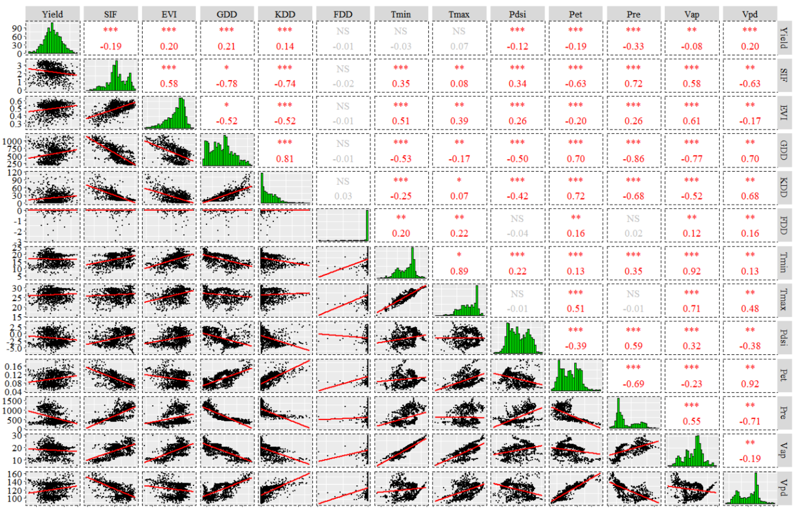
3.2. Spatiotemporal Correlation Patterns between the Transient Variables and Yield

To further investigate the relationships of explanatory variables and yield, we conducted a spatiotemporal correlation analysis between the transient variables and yield. The results showed that the temporal patterns of correlations were almost equivalent for all variables, while the spatial ones differed remarkably among AEZs, suggesting individual models should be developed for each zone.

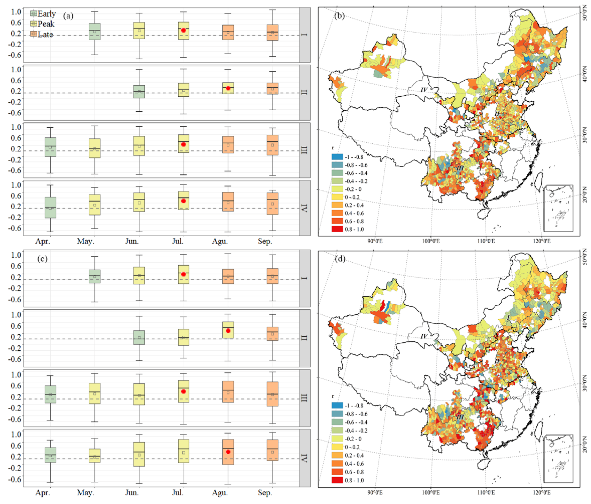
3.2.1. Correlations between Satellite Variables and Yield

Both variables (EVI and SIF) were positively correlated with yield regardless of AEZs and shared the same temporal pattern as the correlations were consistently maximized at the peak stage except for that of SIF in zone IV (Figure 3a,c). The maximums for both data were comparable across AEZs, with the exception of zone II in which SIFs were larger than those of EVI (Figure 3a,c). In contrast, the spatial correlation patterns varied in AEZs. For example, the correlations between SIF and yield were negative for more than 47% of the counties in zone I, and the absolute values were generally less than 0.4 (Figure 3d). However, the correlations in zone II were mostly positive and the coefficients of 30% of counties were higher than 0.6. Similar results were found in zone III for approximately 38% of counties. In comparison with the above three zones, the correlations in zone IV were mostly positive but with a larger variability (Agu. in Figure 3c), which mainly ascribed to the high variability of SIF in northwest China [44]. Similar patterns of EVI were found as that of SIF, and the discrepancy was that more than 50% of counties correlated positively with yield in zone I while negatively for one-third of counties in zone II (Figure 3b).

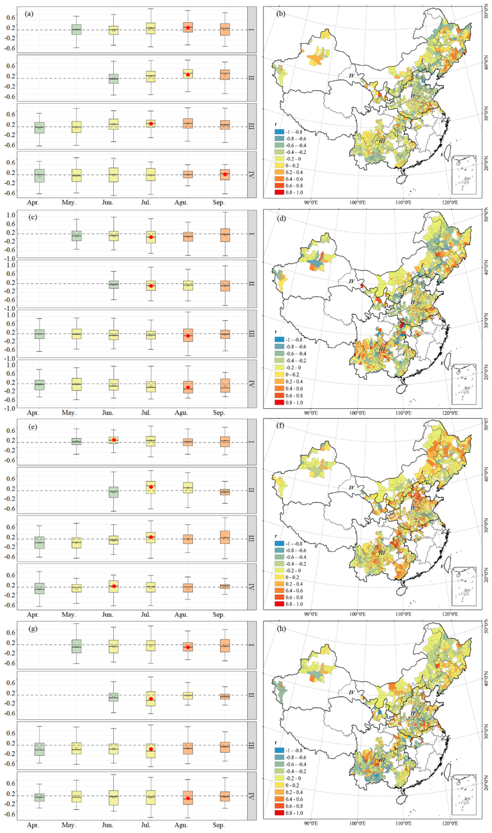
3.2.2. Correlations between Climate Variables and Yield

Similarly to those of satellite data, the maximum absolute values of correlation coefficients were consistently indicated by the peak or late stage for all climate variables, but the values were generally smaller than those of satellite data (Figure 4a,c,e,g). Surprisingly, we found mostly negative correlations with yield for both GDD and KDD (Figure 4a,c). This was most likely due to GDD containing extremely high temperature information, as demonstrated by the significantly linear relationship between the two variables (Figure 2). In contrast, water-related variables (i.e., Pre and Vpd) had a relatively smaller correlation with yield (Figure 4e,g). Precipitation had a positive correlation while negative for Vpd, and the absolute maximum coefficients for Vpd were higher than that for precipitation, suggesting that water-related variables significantly affect maize production [58,60]. As for their spatial patterns (Figure 4b,d,f,h), no climate variables showed obvious differences among the agricultural zones, possibly due to their relatively low temporal and spatial resolutions and, hence, incapability for capturing the spatial variability of environments.

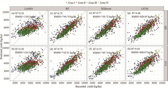
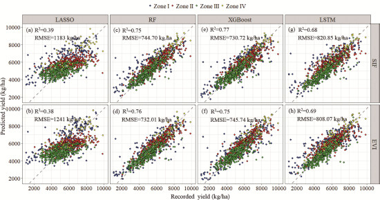
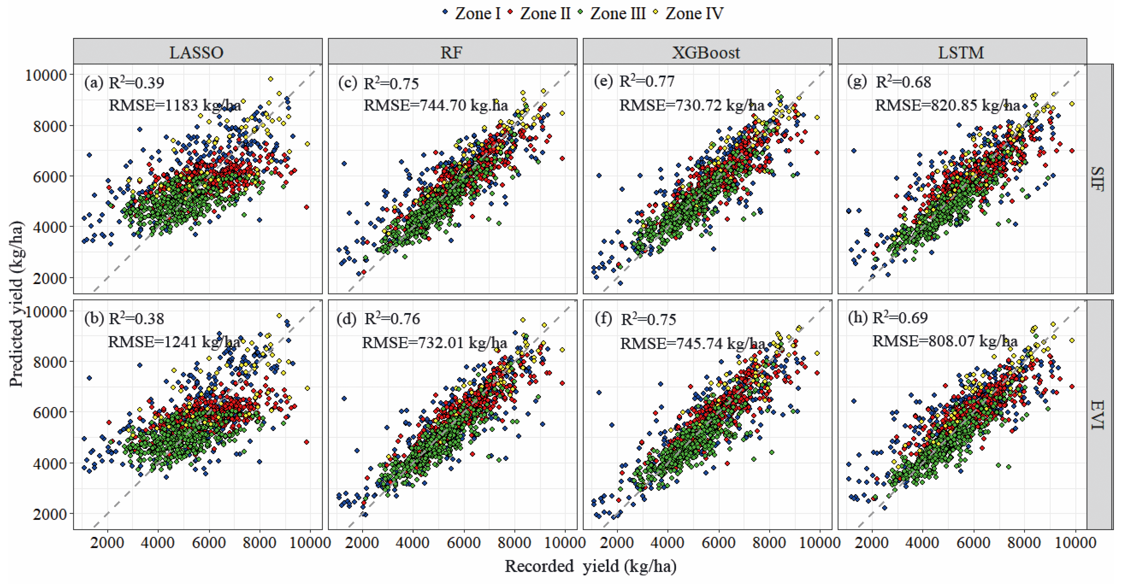
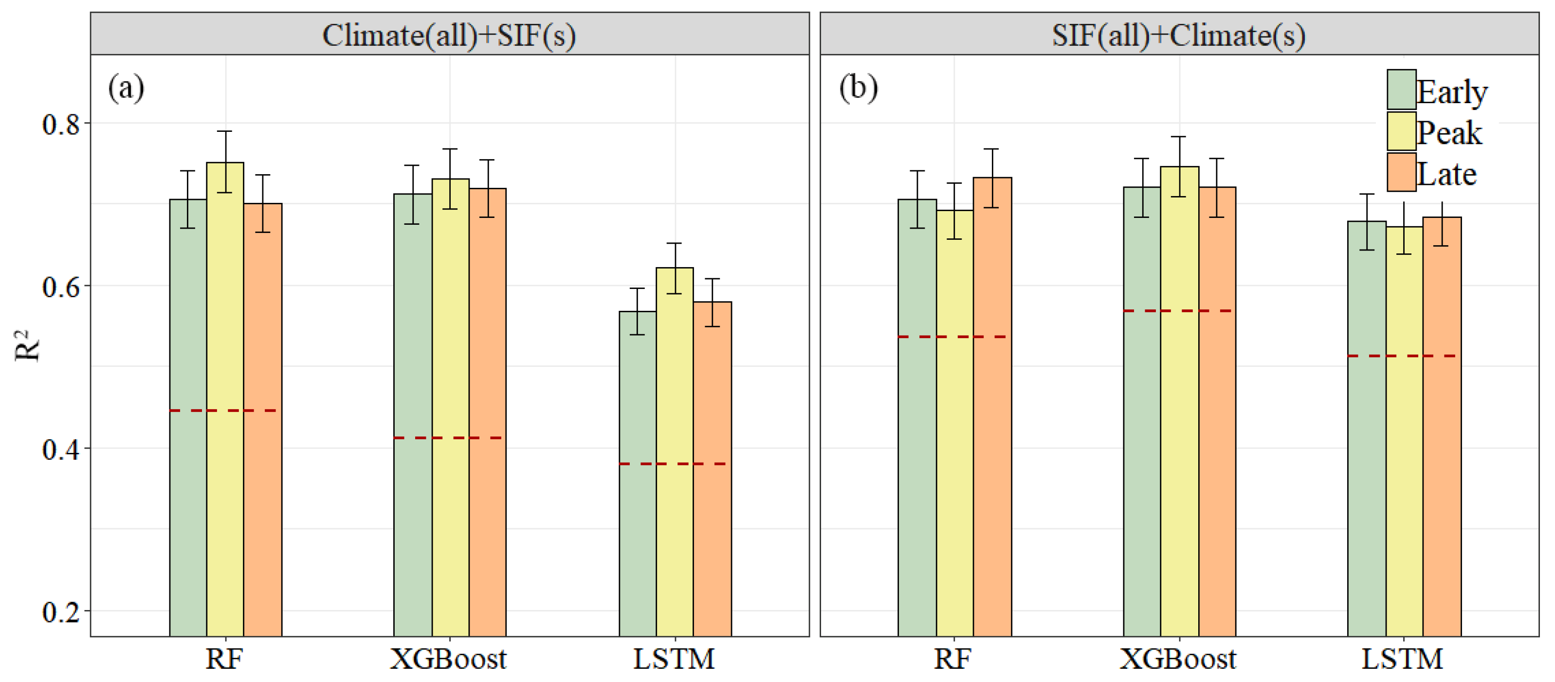
3.3. The Model Performances for Yield Predictions

As shown in Figure 5, on the national scale, SIF and EVI had comparable performances for predicting final yields, demonstrated by the almost equivalent R² for all models. In fact, a slightly higher R² for SIF was found than that of EVI across AEZs with the exception of zone III (Table S6), largely due to the low signal–noise ratio of SIF in southwest China [44]. In agreement with previous studies, ML and DL methods distinctly outperformed the linear regression (i.e., LASSO), independent of input variables and AEZs. We attributed the better performances of ML and DL than LASSO to their ability in capturing potential complex relationships between explanatory variables and yield. The accuracies of the two ML models were relatively higher, which could explain more than 75% of yield variations (Figure 5c,d,e,f). The RMSEs ranged from 731 to 746 kg/ha, which were considerably low compared with the mean of recorded yields (7538 kg/ha). We noticed that the performance of ML models (Figure 5c,d,e,f) were slightly better than LSTM (Figure 5g,h). Please note that the superior performances of ML over LSTM were more obvious in zone IV (Table S2), which might be caused by the relatively small training samples; hence, the LSTM network was incapable of extracting key features. Overall, the performances of SIF and EVI in predicting county-level maize yield were comparable, and the ML and DL methods evidently outperformed traditional linear regression. Based on the above findings, we would only use SIF as a satellite variable and focus on three nonlinear methods in the following analyses.

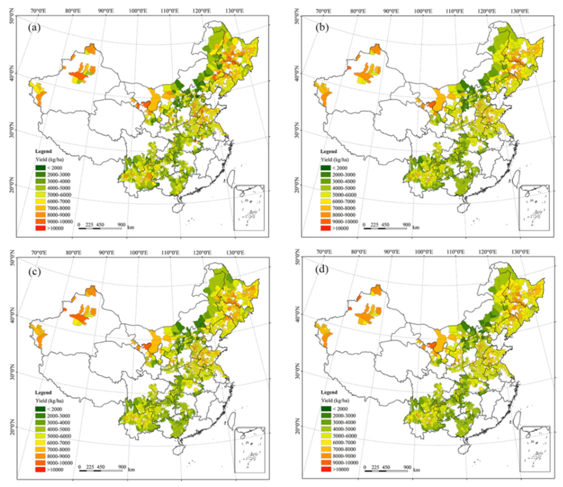
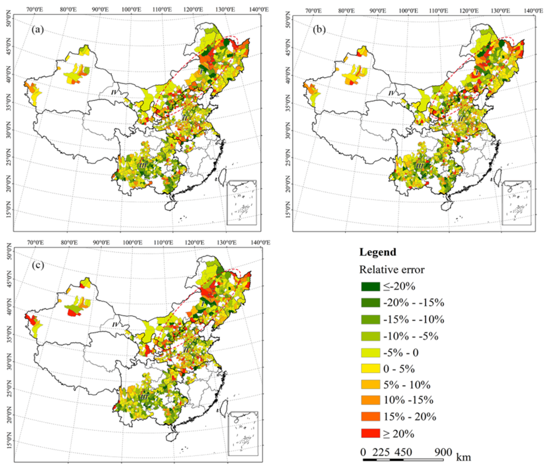
3.4. The Spatial Patterns of Predicted Yield

In China, the high-yield counties were mostly distributed in the northeast, North China Plain, and northwest areas (Figure 6a). However, the counties with the lowest yield were mainly concentrated in the farming–grazing transitional zone in northern China (Figure 6a). The spatial patterns of the predicted yields were in agreement with the reality (recorded ones) for all methods (Figure 6a,b,c,d), demonstrating that ML and DL methods were applicable for crop yield estimation at a larger scale. Moreover, we found the counties with high yields were slightly underestimated, regardless of methods, which were mostly located in northeast China, North China Plain, and Sichuan Basin. The spatial patterns of relative errors for three methods were considerably similar across all AEZs, with the exception of zone IV, in which the errors of the LSTM were higher than the others (Figure 7). The largest errors were consistently found in the farming–grazing transitional zone in northern China, with >20% errors for a quarter of the counties. We attributed the largest errors to frequent disturbance from mixed pixels mainly caused by maize and pasture in the 1 km grid. Similar spatial patterns were found for EVI (Figure S6) but with slightly higher errors than those of SIF (Figure S7).

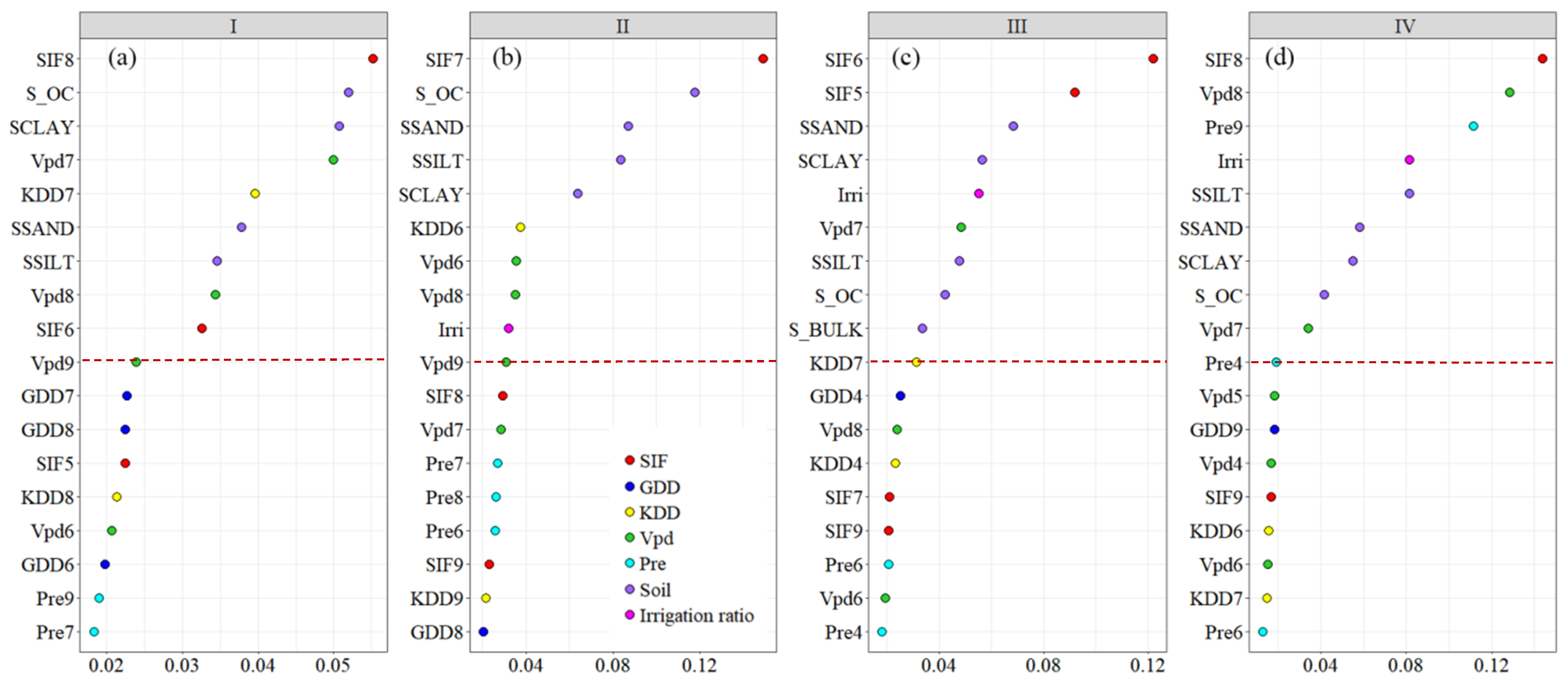
3.5. The Important Factors for Maize Yield Prediction

Figure 8 showed the predicted R²s of three models with one specific stage of SIF combined with all climate variables and other data (Figure 8a) or with one specific stage of climate variables combined with all SIF and other data (Figure 8b). We found that SIF combined with static environmental variables (i.e., soil properties and irrigation ratio, but no any climate input), achieved better results than that climate data did (the dashed lines in Figure 8a,b) regardless of model methods, indicating that satellite data (SIF) provided more information for yield prediction. Combining SIF with all environmental data (i.e., climate data, soil properties, and irrigation ratio) significantly improved the predicted R²s (ranging from 0.19 to 0.32) depending on the methods (Figure 8a). Moreover, the peak SIF consistently showed more contribution than the other two stages, which was in agreement with previous studies [17,29]. In contrast, adding climate information to the combinations of SIF and other static environment variables improved the model performance less, with an R² increase of 0.15–0.20. The peak or late of climate data contributed more information to yield prediction than that of the early stage, which was in accord with the fact that climate conditions during the silking and maturity period most significantly influenced final yield formation [61,62].

To identify the critical factors for maize yield prediction in each AEZ, we further analyzed the important orders of the top 18 variables from the XGBoost models (Figure 9). The peak SIF was consistently ranked as the top one factor for predicting the final yield, followed by soil properties across all AEZs except zone IV. Excluding zone I, irrigation ratios were also ranked in the top 10 across AEZs, suggesting that management practices significantly affected maize production in China [62,63]. However, the order of climate variables was varied among AEZs. In zone I and III (Figure 9a,c), the peak Vpd and KDD were ranked in the top 10. However, climate variables were consistently more important than SIF and soil properties in zone II (Figure 9b), which was in line with those reports in the North China Plain [42,58]. Moreover, the critical climate variables were similar to those in zone I and III, but with the slight differences in the month of KDD and Vpd (Vpd6 and KDD6). Different from the above three zones, we noticed that the top one factor (SIF) was followed by water-related variables (Vpd8 and Pre9) rather than soil properties in zone IV (Figure 9d), highlighting the significant roles of the water-related variables for maize production in northwest China.

4. Discussion

4.1. Comparing the Performances of EVI and SIF in Predicting Crop Yield

In agreement with previous studies [17,64,65], we found both SIF and EVI were positively correlated with yield across AEZs, and the correlation coefficients at the peak stage for SIF were generally higher than that for EVI, illustrating SIF was more sensitive to a high photosynthesis rate. However, we noticed the predicted R² for two data sources were comparable on the national scale irrelative to methods. Such findings could be explained by the following reasons. Firstly, the retrieved SIF contain more uncertainties than VIs [66,67,68]. Secondly, aggregating four-day SIF to a monthly scale weakened its advantages in capturing mild and short-term crop stresses. On the other hand, two data sources may share some information related to aboveground crop biomass because EVI was sensitive to changes in green leaf structure, chlorophyll content, and biomass [17,29,69]. Furthermore, the currently available SIF data might fail in capturing spatial features in details due to a coarse spatial resolution (0.05–1°) relative to EVI (1 km) [70,71,72]. Although SIF data with improved spatial-temporal resolution were used, the issue has not completely been resolved in this study. Overall, SIF was a feasible data source for crop yield estimation at a larger scale, and it was not inferior to EVI.

4.2. Comparing the Performances of Linear, ML, and DL Methods in Predicting Crop Yield

The results showed that ML and DL methods definitely outperformed linear regression (LASSO) across AEZs, largely attributed to their ability to extract the complicated relationships between the predictors and the target variable [14,17,73]. Intuitively, we noticed that ML methods had better performance than the LSTM network across AEZs, especially in zone IV. The difference between ML and DL was mainly caused by fewer maize planting counties there than other zones, consequently resulting in a small training sample in zone IV and subsequently limiting the DL network performance. Furthermore, the DL method can automatically extract key features from input data; however, hand-designed features were used in the study, and the potential power of DL might not be sufficiently utilized [18,48,74,75]. Finally, although our study covered 1198 counties over a 15-year time period (2001–2015), the training samples were relatively small, and thus, combining feature engineering with ML methods could achieve better performance [22,76]. In summary, ML and DL methods evidently outdo statistical regression, and ML has the advantages of computational efficiency and spatial generalization relative to the DL network. In comparison with traditional yield prediction methods (i.e., crop models simulation and statistical regression), they provide new opportunities for yield predictions at regional or even global scales.

4.3. Integrating Multi-Source Data to Predict Large-Scale Crop Yield

Visible and NIR-based VIs are widely prevailed because of their relatively long-time series and high-spatial resolution [9,77]. However, satellite data from other spectra can provide additional information related to crop growth and development [6,78,79]. Furthermore, other factors, such as climate variables and soil properties, significantly affecting crop yield, contain abiotic information, and may not be captured by satellite data [25,80,81]. This study integrated multi-band satellite data with environmental variables to predict county-level maize yield in China. One of the objectives was to investigate which combinations of input variables could achieve the best crop yield prediction.

The results showed that satellite data provided more information and newly detected SIF had a slightly better performance than EVI, which was largely attributed to the fPAR, and the fluorescence yield was sensitive to root zone soil moisture, and thus, added extra information about drought and heat stress [57,78,82]. Moving to thermal bands, LST-based GDD and KDD were both significantly correlated with yield, and were more sensitive to crop water conditions relative to Tair across AEZs, indicating LST can be an indicator of crop water stress, which was supported by previous studies [32,83,84].

We found the combination of SIF and static environmental variables achieved better yield predictions than using environmental data only (i.e., climate variables, soil properties, and irrigation ratio). Adding peak or late of climate information on the top of them could further improve model performance. Although satellite data do show advantages in monitoring crop biomass, final yield is determined by grain weight, which is related to grain number in the flowering period and individual grain size in the grain-filling period [85]. Additionally, numerous agronomy experiments have shown that drought and heat in the above periods have a greater impact on crop growth [86,87]. These findings have explained why adding the silking or maturity stage of climate factors significantly improved crop yield prediction in current study. Beyond satellite and climate data, soil properties should be considered for estimating crop yield at regional scales. The reason was that they contained unique and extra information related to environmental stress on crop growth [39,40,41,42]. Therefore, we suggested that large-scale crop yield prediction should integrate satellite data from different spectral bands and various environmental variables.

4.4. Uncertainties in the Study

This study would also be plagued with some uncertainties. One of the concerns is that SIF suffers from a low signal–noise ratio and coarse spatiotemporal resolution [29,65,66]. With the newly launched TROPOMI onboard the Sentinel 5 (launched on October 13, 2017) [88], the ESA Sentinel-4/UVN instrument (to be launched in 2019) [89] and the FLuorescence EXplorer (FLEX) (to be launched in 2022) [90] SIF with higher spatial and temporal resolution are expected. In addition, the current study focused on predicting county-level crop yield because yield data recorded are only available at the county level. On the other side, most of the satellite datasets in this study are of relatively coarse spatial resolution, resulting in small training samples and limiting the power of ML and DL methods. Finally, ML and DL approaches are “black box” with limited process-based interpretation. Integrating a process-based model with data-driven approaches could not only attain interpretable ML/DL models but, more importantly, are computational efficiency and readily extrapolate outside the range of training conditions [18,91], which is recommended for future large-scale yield estimation, management optimization, and disaster monitoring.

5. Conclusions

In this study, we integrated optical, fluorescence, thermal satellite, and environmental data and employed four data-driven approaches (LASSO, RF, XGBoost, and LSTM) to predict county-level maize yield in China. Results showed that SIF had comparable performance with EVI in predicting crop yield, largely due to the low signal-to-noise ratio and coarse spatial resolution. Thermal-based LST metrics significantly correlated with yield and were sensitive to water conditions relative to Tair, demonstrating they are good indicators of crop water stress. SIF-combined static environmental variables (i.e., soil properties and irrigation ratio) reasonably estimated the final yield, and adding the peak or late of climate information could further improve the model performance. We found that the ML and DL methods evidently outperformed traditional regression models. Moreover, ML methods have advantages of computational efficiency and spatial generalizations relative to the DL network, which opens up new prospects for crop yield prediction at a regional, even global scale. Our study highlights the necessity of integrating multi-spectral satellite data and environmental variables for predicting crop yield on large spatial scales.

References

1. Cole, M.B.; Augustin, M.A.; Robertson, M.J.; Manners, J.M. The science of food security. NPJ Sci. Food 2018, 2, 14. [Google Scholar] [CrossRef] [PubMed]
2. Stevens, T.; Madani, K. Future climate impacts on maize farming and food security in Malawi. Sci. Rep. 2016, 6, 36241. [Google Scholar] [CrossRef] [PubMed] [Green Version]
3. Tilman, D.; Balzer, C.; Hill, J.; Befort, B.L. Global food demand and the sustainable intensification of agriculture. Proc. Natl. Acad. Sci. USA 2011, 108, 20260–20264. [Google Scholar] [CrossRef] [PubMed] [Green Version]
4. Yang, Y.; Xu, W.; Hou, P.; Liu, G.; Liu, W.; Wang, Y.; Zhao, R.; Ming, B.; Xie, R.; Wang, K.; et al. Improving maize grain yield by matching maize growth and solar radiation. Sci. Rep. 2019, 9, 3635. [Google Scholar] [CrossRef] [Green Version]
5. Becker-Reshef, I.; Vermote, E.; Lindeman, M.; Justice, C. A generalized regression-based model for forecasting winter wheat yields in Kansas and Ukraine using MODIS data. Remote Sens. Environ. 2010, 114, 1312–1323. [Google Scholar] [CrossRef]
6. Lambert, M.J.; Traoré, P.C.S.; Blaes, X.; Baret, P.; Defourny, P. Estimating smallholder crops production at village level from Sentinel-2 time series in Mali’s cotton belt. Remote Sens. Environ. 2018, 216, 647–657. [Google Scholar] [CrossRef]
7. Qader, S.H.; Dash, J.; Atkinson, P.M. Forecasting wheat and barley crop production in arid and semi-arid regions using remotely sensed primary productivity and crop phenology: A case study in Iraq. Sci. Total. Environ. 2018, 613, 250–262. [Google Scholar] [CrossRef] [Green Version]
8. Tao, F.; Rotter, R.P.; Palosuo, T.; Gregorio Hernandez Diaz-Ambrona, C.; Minguez, M.I.; Semenov, M.A.; Kersebaum, K.C.; Nendel, C.; Specka, X.; Hoffmann, H.; et al. Contribution of crop model structure, parameters and climate projections to uncertainty in climate change impact assessments. Glob. Chang. Biol. 2018, 24, 1291–1307. [Google Scholar] [CrossRef]
9. Kang, Y.; Özdoğan, M. Field-level crop yield mapping with Landsat using a hierarchical data assimilation approach. Remote Sens. Environ. 2019, 228, 144–163. [Google Scholar] [CrossRef]
10. Folberth, C.; Baklanov, A.; Balkovič, J.; Skalský, R.; Khabarov, N.; Obersteiner, M. Spatio-temporal downscaling of gridded crop model yield estimates based on machine learning. Agric. Meteorol. 2019, 264, 1–15. [Google Scholar] [CrossRef] [Green Version]
11. Rosenzweig, C.; Ruane, A.C.; Antle, J.; Elliott, J.; Ashfaq, M.; Chatta, A.A.; Ewert, F.; Folberth, C.; Hathie, I.; Havlik, P.; et al. Coordinating AgMIP data and models across global and regional scales for 1.5 degrees C and 2.0 degrees C assessments. Philos. Trans. A Math. Phys. Eng. Sci. 2018, 376, 20160455. [Google Scholar] [CrossRef]
12. Pede, T.; Mountrakis, G.; Shaw, S.B. Improving corn yield prediction across the US Corn Belt by replacing air temperature with daily MODIS land surface temperature. Agric. Meteorol. 2019, 276–177, 107615. [Google Scholar] [CrossRef]
13. Lee, J.H.; Shin, J.; Realff, M.J. Machine learning: Overview of the recent progresses and implications for the process systems engineering field. Comput. Chem. Eng. 2018, 114, 111–121. [Google Scholar] [CrossRef]
14. Crane-Droesch, A. Machine learning methods for crop yield prediction and climate change impact assessment in agriculture. Environ. Res. Lett. 2018, 13, 114003. [Google Scholar] [CrossRef] [Green Version]
15. Wang, S.; Azzari, G.; Lobell, D.B. Crop type mapping without field-level labels: Random forest transfer and unsupervised clustering techniques. Remote Sens. Environ. 2019, 222, 303–317. [Google Scholar] [CrossRef]
16. Hunt, M.L.; Blackburn, G.A.; Carrasco, L.; Redhead, J.W.; Rowland, C.S. High resolution wheat yield mapping using Sentinel-2. Remote Sens. Environ. 2019, 233, 111410. [Google Scholar] [CrossRef]
17. Cai, Y.; Guan, K.; Lobell, D.; Potgieter, A.B.; Wang, S.; Peng, J.; Xu, T.; Asseng, S.; Zhang, Y.; You, L.; et al. Integrating satellite and climate data to predict wheat yield in Australia using machine learning approaches. Agric. For. Meteorol. 2019, 274, 144–159. [Google Scholar] [CrossRef]
18. Reichstein, M.; Camps-Valls, G.; Stevens, B.; Jung, M.; Denzler, J.; Carvalhais, N.; Prabhat. Deep learning and process understanding for data-driven Earth system science. Nature 2019, 566, 195–204. [Google Scholar] [CrossRef]
19. Schmidhuber, J. Deep learning in neural networks: An overview. Neural networks. 2015, 61, 85–117. [Google Scholar] [CrossRef] [Green Version]
20. Washburn, J.D.; Mejia-Guerra, M.K.; Ramstein, G.; Kremling, K.A.; Valluru, R.; Buckler, E.S.; Wang, H. Evolutionarily informed deep learning methods for predicting relative transcript abundance from DNA sequence. Proc. Natl. Acad. Sci. USA 2019, 116, 5542–5549. [Google Scholar] [CrossRef] [Green Version]
21. Fischer, T.; Krauss, C. Deep learning with long short-term memory networks for financial market predictions. Eur. J. Oper. Res. 2018, 270, 654–669. [Google Scholar] [CrossRef] [Green Version]
22. Kuwata, K.; Shibasaki, R. Estimating crop yields with deep learning and remotely sensed data. In Proceedings of the 2015 IEEE International Geoscience and Remote Sensing Symposium (IGARSS), Milan, Italy, 26–31 July 2015; pp. 858–861. [Google Scholar]
23. Jin, Z.; Azzari, G.; Burke, M.; Aston, S.; Lobell, D. Mapping Smallholder Yield Heterogeneity at Multiple Scales in Eastern Africa. Remote Sens. 2017, 9, 931. [Google Scholar] [CrossRef] [Green Version]
24. Kern, A.; Barcza, Z.; Marjanović, H.; Árendás, T.; Fodor, N.; Bónis, P.; Bognár, P.; Lichtenberger, J. Statistical modelling of crop yield in Central Europe using climate data and remote sensing vegetation indices. Agric. For. Meteorol. 2018, 260, 300–320. [Google Scholar] [CrossRef]
25. Azzari, G.; Jain, M.; Lobell, D. Towards fine resolution global maps of crop yields: Testing multiple methods and satellites in three countries. Remote Sens. Environ. 2017, 202, 129–141. [Google Scholar] [CrossRef]
26. Dong, J.; Xiao, X.; Wagle, P.; Zhang, G.; Zhou, Y.; Jin, C.; Torn, M.S.; Meyers, T.P.; Suyker, A.E.; Wang, J.; et al. Comparison of four EVI-based models for estimating gross primary production of maize and soybean croplands and tallgrass prairie under severe drought. Remote Sens. Environ. 2015, 162, 154–168. [Google Scholar] [CrossRef] [Green Version]
27. Song, L.; Guanter, L.; Guan, K.; You, L.; Huete, A.; Ju, W.; Zhang, Y. Satellite sun-induced chlorophyll fluorescence detects early response of winter wheat to heat stress in the Indian Indo-Gangetic Plains. Glob Chang. Biol. 2018, 24, 4023–4037. [Google Scholar] [CrossRef] [Green Version]
28. Sun, Y.; Fu, R.; Dickinson, R.; Joiner, J.; Frankenberg, C.; Gu, L.; Xia, Y.; Fernando, N. Drought onset mechanisms revealed by satellite solar-induced chlorophyll fluorescence: Insights from two contrasting extreme events. J. Geophys. Res. Biogeosciences 2015, 120, 2427–2440. [Google Scholar] [CrossRef]
29. Guan, K.; Wu, J.; Kimball, J.S.; Anderson, M.C.; Frolking, S.; Li, B.; Hain, C.R.; Lobell, D. The shared and unique values of optical, fluorescence, thermal and microwave satellite data for estimating large-scale crop yields. Remote Sens. Environ. 2017, 199, 333–349. [Google Scholar] [CrossRef] [Green Version]
30. He, M.; Kimball, J.S.; Yi, Y.; Running, S.; Guan, K.; Jensco, K.; Maxwell, B.; Maneta, M. Impacts of the 2017 flash drought in the US Northern plains informed by satellite-based evapotranspiration and solar-induced fluorescence. Environ. Res. Lett. 2019, 14, 074019. [Google Scholar] [CrossRef] [Green Version]
31. Holzman, M.E.; Carmona, F.; Rivas, R.; Niclòs, R. Early assessment of crop yield from remotely sensed water stress and solar radiation data. ISPRS J. Photogramm. Remote Sens. 2018, 145, 297–308, S0924271618300790. [Google Scholar] [CrossRef]
32. Hu, X.; Ren, H.; Tansey, K.; Zheng, Y.; Ghent, D.; Liu, X.; Yan, L. Agricultural drought monitoring using European Space Agency Sentinel 3A land surface temperature and normalized difference vegetation index imageries. Agric. For. Meteorol. 2019, 279, 107707. [Google Scholar] [CrossRef]
33. Shivers, S.W.; Roberts, D.A.; McFadden, J.P. Using paired thermal and hyperspectral aerial imagery to quantify land surface temperature variability and assess crop stress within California orchards. Remote Sens. Environ. 2019, 222, 215–231. [Google Scholar] [CrossRef]
34. Heft-Neal, S.; Lobell, D.; Burke, M. Using remotely sensed temperature to estimate climate response functions. Environ. Res. Lett. 2017, 12, 014013. [Google Scholar] [CrossRef] [Green Version]
35. Piao, S.; Ciais, P.; Huang, Y.; Shen, Z.; Peng, S.; Li, J.; Zhou, L.; Liu, H.; Ma, Y.; Ding, Y.; et al. The impacts of climate change on water resources and agriculture in China. Nature 2010, 467, 43–51. [Google Scholar] [CrossRef]
36. Mueller, N.D.; Gerber, J.S.; Johnston, M.; Ray, D.K.; Ramankutty, N.; Foley, J.A. Closing yield gaps through nutrient and water management. Nature 2012, 490, 254–257. [Google Scholar] [CrossRef]
37. Shaw, S.B.; Mehta, D.; Riha, S.J. Using simple data experiments to explore the influence of non-temperature controls on maize yields in the mid-West and Great Plains. Clim. Change 2014, 122, 747–755. [Google Scholar] [CrossRef]
38. Troy, T.J.; Kipgen, C.; Pal, I. The impact of climate extremes and irrigation on US crop yields. Environ. Res. Lett. 2015, 10, 054013. [Google Scholar] [CrossRef] [Green Version]
39. Kiboi, M.N.; Ngetich, K.F.; Fliessbach, A.; Muriuki, A.; Mugendi, D.N. Soil fertility inputs and tillage influence on maize crop performance and soil water content in the Central Highlands of Kenya. Agric. Water Manag. 2019, 217, 316–331. [Google Scholar] [CrossRef]
40. Zhang, Y.; Wang, R.; Wang, H.; Wang, S.; Wang, X.; Li, J. Soil water use and crop yield increase under different long-term fertilization practices incorporated with two-year tillage rotations. Agric. Water Manag. 2019, 221, 362–370. [Google Scholar] [CrossRef]
41. Chen, Y.; Zhang, Z.; Tao, F.; Wang, P.; Wei, X. Spatio-temporal patterns of winter wheat yield potential and yield gap during the past three decades in North China. Field Crop. Res. 2017, 206, 11–20. [Google Scholar] [CrossRef]
42. Zhao, J.; Yang, X.; Sun, S. Constraints on maize yield and yield stability in the main cropping regions in China. Eur. J. Agron. 2018, 99, 106–115. [Google Scholar] [CrossRef]
43. Luo, Y.; Zhang, Z.; Chen, Y.; Li, Z.; Tao, F. ChinaCropPhen1km: A high-resolution crop phenological dataset for three staple crops in China during 2000–2015 based on LAI products. Earth Syst. Sci. Data Discuss. 2019. in review. [Google Scholar] [CrossRef]
44. Zhang, Y.; Joiner, J.; Alemohammad, S.H.; Zhou, S.; Gentine, P. A global spatially contiguous solar-induced fluorescence (CSIF) dataset using neural networks. Biogeosciences 2018, 15, 5779–5800. [Google Scholar] [CrossRef] [Green Version]
45. Schauberger, B.; Gornott, C.; Wechsung, F. Global evaluation of a semiempirical model for yield anomalies and application to within-season yield forecasting. Glob. Chang. Biol. 2017, 23, 4750–4764. [Google Scholar] [CrossRef]
46. Abatzoglou, J.T.; Dobrowski, S.Z.; Parks, S.A.; Hegewisch, K.C. Terraclimate, a high-resolution global dataset of monthly climate and climatic water balance from 1958–2015. Sci. Data. 2018, 5, 170191. [Google Scholar] [CrossRef] [Green Version]
47. Shangguan, W.; Dai, Y.; Liu, B.; Ye, A.; Yuan, H. A soil particle-size distribution dataset for regional land and climate modelling in china. Geoderma 2012, 171, 85–91. [Google Scholar] [CrossRef]
48. Lecun, Y.; Bengio, Y.; Hinton, G. Deep learning. Nature 2015, 521, 436. [Google Scholar] [CrossRef]
49. Tibshirani, R. Regression shrinkage and selection via the lasso. J. R. Stat. Soc. 1996, 58, 267–288. [Google Scholar] [CrossRef]
50. Breiman, L. Random forests. Mach. Learn. 2001, 45, 5–32. [Google Scholar] [CrossRef] [Green Version]
51. Chen, T.; Guestrin, C. Xgboost: A scalable tree boosting system. In Proceedings of the 22nd Acm Sigkdd International Conference on Knowledge Discovery and Data Mining, San Francisco, CA, USA, 13–17 August 2016; pp. 785–794. [Google Scholar]
52. Hochreiter, S.; Schmidhuber, J. Long short-term memory. Neural Comput. 1997, 9, 1735–1780. [Google Scholar] [CrossRef]
53. Sak, H.; Senior, A.; Beaufays, F. Long short-term memory based recurrent neural network architectures for large vocabulary speech recognition. arXiv 2014, arXiv:1402.1128. [Google Scholar]
54. He, T.; Xie, C.; Liu, Q.; Guan, S.; Liu, G. Evaluation and comparison of random forest and A-LSTM networks for large-scale winter wheat identification. Remote Sens. 2019, 11, 1665. [Google Scholar] [CrossRef] [Green Version]
55. Lesk, C.; Rowhani, P.; Ramankutty, N. Influence of extreme weather disasters on global crop production. Nature 2016, 529, 84–87. [Google Scholar] [CrossRef] [PubMed]
56. Ma, J.; Maystadt, J.F. The impact of weather variations on maize yields and household income: Income diversification as adaptation in rural china. Glob. Environ. Chang. 2017, 42, 93–106. [Google Scholar] [CrossRef] [Green Version]
57. Liu, B.; Chen, X.; Meng, Q.; Yang, H.; Wart, J.V. Estimating maize yield potential and yield gap with agro-climatic zones in china—distinguish irrigated and rainfed conditions. Agric. For. Meteorol. 2017, 239, 108–117. [Google Scholar] [CrossRef]
58. Zhao, J.; Yang, X. Distribution of high-yield and high-yield-stability zones for maize yield potential in the main growing regions in china. Agric. For. Meteorol. 2018, 248, 511–517. [Google Scholar] [CrossRef]
59. Zhang, H.; Tao, F.; Zhou, G. Potential yields, yield gaps, and optimal agronomic management practices for rice production systems in different regions of china. Agric. Syst. 2019, 171, 100–112. [Google Scholar] [CrossRef]
60. Mathieu, J.A.; Aires, F. Assessment of the agro-climatic indices to improve crop yield forecasting. Agric. For. Meteorol. 2018, 253, 15–30. [Google Scholar] [CrossRef]
61. Tao, F.; Zhang, S.; Zhang, Z.; Rötter, R.P. Temporal and spatial changes of maize yield potentials and yield gaps in the past three decades in china. Agric. Ecosyst. Environ. 2015, 208, 12–20. [Google Scholar] [CrossRef]
62. Liu, Y.; Chen, Q.; Ge, Q.; Dai, J.; Qin, Y.; Dai, L.; Zou, X.T.; Chen, C. Modelling the impacts of climate change and crop management on phenological trends of spring and winter wheat in china. Agric. For. Meteorol. 2017, 248, 518–526. [Google Scholar] [CrossRef]
63. Wang, X.; Li, T.; Yang, X.; Zhang, T.; Lai, Y. Rice yield potential, gaps and constraints during the past three decades in a climate-changing northeast china. Agric. For. Meteorol. 2018, 259, 173–183. [Google Scholar] [CrossRef]
64. Liu, L.; Guan, L.; Liu, X. Directly estimating diurnal changes in GPP for c3 and c4 crops using far-red sun-induced chlorophyll fluorescence. Agric. For. Meteorol. 2017, 232, 1–9. [Google Scholar] [CrossRef]
65. Chen, X.; Mo, X.; Zhang, Y.; Sun, Z.; Liu, Y.; Hu, S.; Liu, S. Drought detection and assessment with solar-induced chlorophyll fluorescence in summer maize growth period over North China Plain. Ecol. Indic. 2019, 104, 347–356. [Google Scholar] [CrossRef]
66. Guanter, L.; Zhang, Y.; Jung, M.; Joiner, J.; Voigt, M.; Berry, J.A.; Frankenberg, C.; Huete, A.R.; Zarco-te, J.; Pablo, L. Global and time-resolved monitoring of crop photosynthesis with chlorophyll fluorescence. Proc. Natl. Acad. Sci. USA 2014, 111, E1327–E1333. [Google Scholar] [CrossRef] [Green Version]
67. Sun, Y.; Frankenberg, C.; Wood, J.D.; Schimel, D.S.; Jung, M.; Guanter, L.; Dreery, D.T.; Verma, M.; Porcar-Castell, A.; Griffis, T.J. Oco-2 advances photosynthesis observation from space via solar-induced chlorophyll fluorescence. Science 2017, 358, eaam5747. [Google Scholar] [CrossRef] [Green Version]
68. Köhler, P.; Frankenberg, C.; Magney, T.S.; Guanter, L.; Joiner, J.; Landgraf, J. Global Retrievals of Solar-Induced Chlorophyll Fluorescence With TROPOMI: First Results and Intersensor Comparison to OCO-2. Geophys. Res. Lett. 2018, 45, 10456–10463. [Google Scholar]
69. Yoshida, Y.; Joiner, J.; Tucker, C.; Berry, J.; Lee, J.E.; Walker, G.; Reichle, R.; Koster, R.; Lyapustin, A.; Wang, Y. The 2010 Russian drought impact on satellite measurements of solar-induced chlorophyll fluorescence: Insights from modeling and comparisons with parameters derived from satellite reflectances. Remote Sens. Environ. 2015, 166, 163–177. [Google Scholar] [CrossRef]
70. Mohammed, G.H.; Colombo, R.; Middleton, E.M.; Rascher, U.; van der Tol, C.; Nedbal, L.; Goulas, Y.; Pérez-Priego, O.; Damm, A.; Meroni, M.; et al. Remote sensing of solar-induced chlorophyll fluorescence (SIF) in vegetation: 50 years of progress. Remote sens. Environ. 2019, 231, 111177. [Google Scholar] [CrossRef]
71. Guan, K.; Berry, J.A.; Zhang, Y.; Joiner, J.; Guanter, L.; Badgley, G.; Lobell, D. Improving the monitoring of crop productivity using spaceborne solar-induced fluorescence. Glob. Chang. Biol. 2016, 22, 716–726. [Google Scholar] [CrossRef]
72. Wei, J.; Tang, X.; Gu, Q.; Wang, M.; Ma, M.; Han, X. Using Solar-Induced Chlorophyll Fluorescence Observed by OCO-2 to Predict Autumn Crop Production in China. Remote Sens. 2019, 11, 1715. [Google Scholar] [CrossRef] [Green Version]
73. Feng, P.; Wang, B.; Liu, L.; Waters, C.; Yu, Q. Incorporating Machine Learning with Biophysical Model Can Improve the Evaluation of Climate Extremes Impacts on Wheat Yield in South-eastern Australia. Agric. For. Meteorol. 2019, 275, 100–113. [Google Scholar] [CrossRef]
74. Stephan, R.; Pritchard, M.S.; Pierre, G. Deep learning to represent subgrid processes in climate models. Proc. Natl. Acad. Sci. USA 2018, 115, 9684–9689. [Google Scholar]
75. Nevavuori, P.; Narra, N.; Lipping, T. Crop yield prediction with deep convolutional neural networks. Comput. Electron. Agric. 2019, 163, 104859. [Google Scholar] [CrossRef]
76. Yang, Q.; Shi, L.; Han, J.; Zha, Y.; Zhu, P. Deep convolutional neural networks for rice grain yield estimation at the ripening stage using UAV-based remotely sensed images. Field Crop. Res. 2019, 235, 142–153. [Google Scholar] [CrossRef]
77. Zhang, X.; Zhang, Q. Monitoring interannual variation in global crop yield using long-term AVHRR and MODIS observations. ISPRS J. Photogramm. Remote Sens. 2016, 114, 191–205. [Google Scholar] [CrossRef]
78. Yang, K.; Ryu, Y.; Dechant, B.; Berry, J.A.; Hwang, Y.; Jinag, C.; Kang, M.; Kim, J.; Kimm, H.; Kornfeld, A. Sun-induced chlorophyll fluorescence is more strongly related to absorbed light than to photosynthesis at half-hourly resolution in a rice paddy. Remote Sens. Environ. 2018, 216, 658–673. [Google Scholar] [CrossRef]
79. Mateo-Sanchis, A.; Piles, M.; Muñoz-Marí, J.; Adsuara, J.E.; Pérez-Suay, A.; Camps-Valls, G. Synergistic integration of optical and microwave satellite data for crop yield estimation. Remote Sens. Environ. 2019, 234, 111460. [Google Scholar] [CrossRef]
80. Lobell, D.; Thau, D.; Seifert, C.; Engle, E.; Little, B. A scalable satellite-based crop yield mapper. Remote Sens. Environ. 2015, 164, 324–333. [Google Scholar] [CrossRef]
81. Jin, Z.; Azzari, G.; You, C.; Di Tommaso, S.; Aston, S.; Burke, M.; Lobell, D.B. Smallholder maize area and yield mapping at national scales with google earth engine. Remote Sens. Environ. 2019, 228, 115–128. [Google Scholar] [CrossRef]
82. Liu, L.; Yang, X.; Zhou, H.; Liu, S.; Zhou, L.; Li, X.; Yang, J.; Han, X.J.; Wu, J. Evaluating the utility of solar-induced chlorophyll fluorescence for drought monitoring by comparison with NDVI derived from wheat canopy. Sci. Total. Environ. 2018, 625, 1208. [Google Scholar] [CrossRef]
83. Li, H.; Sun, D.; Yu, Y.; Wang, H.; Liu, Y.; Liu, Q.; Du, Y.; Wang, H.; Cao, B. Evaluation of the viirs and modis lst products in an arid area of northwest china. Remote Sens. Environ. 2014, 142, 111–121. [Google Scholar] [CrossRef] [Green Version]
84. Eleftheriou, D.; Kiachidis, K.; Kalmintzis, G.; Kalea, A.; Bantasis, C.; Koumadoraki, P.; Spathara, M.E.; Tsolaki, A.; Tzampazidou, M.I.; Gemitzi, A. Determination of annual and seasonal daytime and nighttime trends of MODIS LST over Greece-climate change implications. Sci. Total. Environ. 2018, 616, 937–947. [Google Scholar] [CrossRef] [PubMed]
85. Katsura, K.; Nakaide, Y. Factors that determine grain weight in rice under high-yielding aerobic culture: The importance of husk size. Field Crop. Res. 2011, 123, 266–272. [Google Scholar] [CrossRef]
86. Benincasa, P.; Reale, L.; Tedeschini, E.; Ferri, V.; Cerri, M.; Ghitarrini, S.; Falcinelli, B.; Frenguelli, G.; Ferranti, F.; Ayano, B.E.; et al. The relationship between grain and ovary size in wheat: An analysis of contrasting grain weight cultivars under different growing conditions. Field Crop. Res. 2017, 210, 175–182. [Google Scholar] [CrossRef]
87. Chen, Y.; Zhang, Z.; Wang, P.; Song, X.; Wei, X.; Tao, F. Identifying the impact of multi-hazards on crop yield—A case for heat stress and dry stress on winter wheat yield in northern china. Eur. J. Agron. 2016, 73, 55–63. [Google Scholar] [CrossRef]
88. Guanter, L.; Aben, I.; Tol, P.; Krijger, J.M.; Hollstein, A.; Köhler, P.; Damm, A.; Joiner, J.J.; Frankenbery, C.; Landgraf, J. Potential of the tropospheric monitoring instrument (tropomi) onboard the sentinel-5 precursor for the monitoring of terrestrial chlorophyll fluorescence. Atmos. Meas. Tech. 2015, 8, 1337–1352. [Google Scholar] [CrossRef] [Green Version]
89. Stark, H.R.; Moeller, H.L.; Courreges-Lacoste, G.B.; Ben Veihelmann, R.K. The Sentinel-4 mission and its implementation. ESA Living Planet. Symp. 2013, 722, 139. [Google Scholar]
90. Moreno, J.F.; Miglietta, F.; Mohammed, G.; Rascher, U.; Middleton, E.; Goulas, Y.; Huth, A.; Kraft, S.; Middleton, E.M.; Miglietta, F.; et al. The fluorescence explorer mission concept—ESA’s earth explorer 8. IEEE Trans. Geosci. Remote Sens. 2016, 55, 1273–1284. [Google Scholar]
91. Murdoch, W.J.; Singh, C.; Kumbier, K.; Abbasi-Asl, R.; Yu, B. Definitions, methods, and applications in interpretable machine learning. Proc. Natl. Acad. Sci. USA 2019, 116, 22071–22080. [Google Scholar] [CrossRef] [Green Version]
Figure 1. The maize planting areas and four main agro-ecological zones in China.
Remotesensing 12 00021 g001
Figure 2. The correlations between yield and the transient variables (i.e., solar-induced chlorophyll (SIF), the enhanced vegetation index (EVI), and climate variables). *, ** and *** represent significance levels of p < 0.05, p < 0.01 and p < 0.001, respectively; “NS” denotes significance levels above 0.05.
Remotesensing 12 00021 g002
Figure 3. Spatiotemporal correlations between satellite variables (EVI, (a,b); SIF, (c,d)) and yield. In the box plot, the horizontal lines show the maximum and minimum values; the middle line shows the median; the upper and lower edges of the boxes show the 75th and 25th percentiles, respectively; the gray square represents the mean; the right part is the spatial pattern of the correlation for the month with the highest correlation coefficient (the red circle in the left part).
Remotesensing 12 00021 g003
Figure 4. Spatiotemporal correlations between the selected climate variables (GDD, (a,b); KDD, (c,d); Pre, (e,f); Vpd, (g,h)) and yield.
Remotesensing 12 00021 g004
Figure 5. Comparison of the recorded and multi-model predicted yields. The R2 and RMSE were ten-fold cross-validated values.
Remotesensing 12 00021 g005
Figure 6. The spatial patterns of the recorded yield (a) and predicted yield for RF (b), XGBoost (c), and LSTM (d).
Remotesensing 12 00021 g006
Figure 7. The spatial patterns of the relative errors for random forest (RF) (a), Extreme gradient boosting (XGBoost) (b), and long short-term memory (LSTM) (c).
Remotesensing 12 00021 g007
Figure 8. (a) R2 for one specific stage of SIF combined with all climate variables and other data. The dashed line represents the result of using environmental data, excluding SIF. (b) R2 for SIF combined with one specific stage of climate variables and other data. The dashed line represents the result of using SIF and other data, excluding climate variables.
Remotesensing 12 00021 g008
Figure 9. Feature importance values for the top of 18 variables from XGBoost models in each agro-ecological zone. The red dashed line indicates the 10th variable.
Remotesensing 12 00021 g009