Mapping Heterogeneous Buried Archaeological Features Using Multisensor Data from Unmanned Aerial Vehicles

1
Department of History, University of Nottingham, Nottingham NG7 2RD, UK
2
School of Animal, Rural and Environmental Sciences, Nottingham Trent University, Southwell, Nottinghamshire NG25 0QF, UK
*
Author to whom correspondence should be addressed.
Remote Sens. 2020, 12(1), 41; https://0-doi-org.brum.beds.ac.uk/10.3390/rs12010041
Submission received: 21 November 2019
/
Revised: 12 December 2019
/
Accepted: 17 December 2019
/
Published: 20 December 2019
(This article belongs to the Special Issue 2nd Edition Advances in Remote Sensing for Archaeological Heritage)
Abstract
:There is a long history of the use of aerial imagery for archaeological research, but the application of multisensor image data has only recently been facilitated by the development of unmanned aerial vehicles (UAVs). Two archaeological sites in the East Midlands U.K. that differ in age and topography were selected for survey using multisensor imaging from a fixed-wing UAV. The aim of this study was to determine optimum methodology for the use of UAVs in examining archaeological sites that have no obvious surface features and examine issues of ground control target design, thermal effects, image processing and advanced filtration. The information derived from the range of sensors used in this study enabled interpretation of buried archaeology at both sites. For any archaeological survey using UAVs, the acquisition of visible colour (RGB), multispectral, and thermal imagery as a minimum are advised, as no single technique is sufficient to attempt to reveal the maximum amount of potential information.
1. Introduction
1.1. Overview
The use of remote sensing to survey and research archaeological sites is well established in the literature [1,2,3,4,5,6,7,8], and although conventional aerial photography and LiDAR are commonplace the use of multisensor data acquisition is less well represented. In this study the authors have selected two separate archaeological sites which differ considerably in character, period, and physical aspect and which both have known multiperiod features. Neither site has previously been extensively studied or excavated.
The aim of the study was to compare the efficacy of multisensor data, acquired aerially from an unmanned aerial vehicle (UAV), in providing adequate visualization of buried archaeology in order to formulate an accurate approximation of each site’s principal features and characteristics. Ground-truthing of the results to date has largely been restricted to visual site inspection owing to the current uses of the land and restrictions by the owners; this is a very commonly encountered scenario in archaeology where non-invasive survey provides the only practical means of determining the nature of man-made, below ground stratigraphy [9,10].
As well as determining the efficacy of the methods employed, the results are, in themselves, of key importance in the understanding of the archaeological nature of the two sites examined. The only available options other than passive aerial remote sensing are geophysical survey, terrestrial laser scanning (TLS) or manual topographic mapping (to reveal any residual elevation differences for detecting ditches and banks), and physical excavation. The latter, though clearly the most informative, is also the most restrictive in terms of both permission and cost, and also entails the irreversible destruction of the archaeology, which should be avoided where possible. For the first site in this study, Camp Hill, geophysics, TLS and manual surveying, whilst being possible, would entail considerable time and logistics owing to the extent and nature of the terrain and are, for all practical purposes, unfeasible. Therefore, this study also aims to present interpretations of the two sites selected which have hitherto not been attempted.
1.2. Archaeological Background
The two sites selected for study are in Nottinghamshire, U.K.: (a) Camp Hill, Hexgreave Park; and (b) Shelford Priory (Figure 1 and Figure 2).
1.2.1. Camp Hill
Camp Hill is a complex archaeological site, most probably an Iron Age hillfort comprising the largest in a group of local hillforts in central Nottinghamshire, U.K (Figure 1); such clusters of hillforts are well known from elsewhere in Europe [11]. It lies at 67 m above sea level (asl) surrounding a low-lying hill. In extent the outer ditch, insofar as may be determined from ground survey and aerial photography, encloses an area of approximately 42 ha, which is unusually large for this class of structure; for comparison, the well-studied and preserved hillfort at Maiden Castle, Dorset, U.K. is approximately 45 ha in extent and the equally well preserved site of Hod Hill, 29 km N.E., is in the region of 30 ha. A single find of a late Neolithic-Early Bronze-Age flint tool may indicate the earlier origins of the site, whilst a prolific scatter of Roman and Romano-British pottery, along with a Roman road cutting through the hillfort, demonstrate later continuation of use. The area adjacent to the west was further developed as a deer park for the archbishops of York in the medieval era, but is excluded from this study.
The geology of the site is largely early to mid-Triassic Tarporley siltstone and the region of interest (ROI) where data was acquired is entirely comprised of this bedrock. The overlying soil type is loam and heavy clay and is arable land, actively farmed with cereal crops and strips of uncultivated field margin, hedges, grass trackways, and a triangle of woodland on the southern edge of the ROI (Figure 2).
The area has been little analysed. First mentioned as an archaeological site in 1677, but not examined until 1788 [12], early drawings show an irregular lozenge with apparent ditches and ramparts on four sides which, in the late 18th century, were clearly still visible. In 1849 a pig of lead bearing a Roman inscription was discovered [13,14,15], and this clearly indicates that the road was being used to transport lead from the Derbyshire mines, probably to the east coast for export. Field walking in the 1930s, 1960s, and in 1974-5 revealed much pottery of Iron Age to 2nd century A.D. date, and unpublished aerial photography was used to discern the faint remaining boundaries of the ditches, which are known to have been destroyed by ploughing during the 19th century [16]. More recently, LiDAR mapping by the U.K. Environment Agency has revealed the partial profile of the inner ditch on the south side of the site, the probable entrance to the fort, and the Roman road; however, the nature of the interior complex has remained elusive as the ground resolution of the LiDAR data is 1 m, and also as many archaeological features evidently do not present as significant topological variations due to extensive past agricultural activity.
1.2.2. Shelford Priory
Shelford Priory was a small Augustinian monastery founded during the reign of King Henry II, between AD 1154 and 1189, and which housed up to 14 canons [17,18]. It was located close to the south bank of the River Trent in Nottinghamshire, U.K. at 19 m asl (Figure 1), and was suppressed during the English Reformation in 1536. After the complex ceased to be used as a religious house it was sold to the Stanhope family who created a house which was damaged during the English Civil War and repaired in 1678. Recent investigations [19] have shown that the current farmhouse was almost certainly the monastic ‘prior’s lodgings’ and retains a considerable amount of the original medieval building. The remainder of the monastery was probably robbed for stone and destroyed.
Of the main complex, including the medieval church, cloister, and related buildings, there are no discernible traces above ground and the 0.85 ha site is a field under pasture (Figure 2). In 2001 a brief archaeological evaluation excavation was undertaken for a U.K. television programme series which centred on the Civil War earthworks thought to also be on the site; unfortunately no published site report has ever been issued, although archive footage and photographs reveal trench excavation of around 0.5 m in depth yielding evidence of medieval buildings, including what appears to be the church at that depth [20]. However, no attempts have ever been made to understand the complex in its entirety.
The geology of the ROI is principally sand and gravel with some slit and clay deposits on the northern edge, and the soil type is mixed sand, loam, and some clay, firm but with very high permeability.
1.3. Background Theory
Aerial Photography in Archaeology
The use of aerial photography to research archaeological sites is well established [21,22,23]. Using conventional camera technology, sites are often revealed due to one of three common processes:
i) Cropmarks: where crops or other vegetation grow at differential rates and heights due to varying ground moisture content that is dependent on the subsurface presence of masonry, pits, ditches, and so forth.
ii) Parch marks: similar to (i) but resulting from intense lack of ground moisture such as during a drought where vegetation above masonry dies back more quickly than surrounding material, resulting in a stark colour contrast.
iii) Shadow marks: where low sun angle produces enhanced relief of the ground surface in the imagery revealing features such as banks, ditches and low wall foundations.
Multispectral and thermal imaging are comparatively recent developments in the archaeological survey toolkit and the availability of UAVs has further enabled the capture of very high spatial resolution imagery—vital for the detection of subtle, man-made features such as buried walls and ditches [24,25,26,27].
The principles of detection are, for multispectral imaging, similar to conventional colour (RGB) data, where differences in crop and vegetation growth, which are dependent on subsurface soil makeup and moisture conditions, are revealed as deviations in colour [28,29] and sometimes as weak localized changes in surface topography [30]. The advantages of using multispectral imaging that includes the near infra-red (NIR) include a wider spectral range for general surface reflection properties and the use of the normalized difference vegetation index (NDVI), which is the differenced ratio of reflectance in the red and near-infrared wavelength [31], to reveal an indication of crop health [32]. The equation for NDVI is given as:
where рnir is the spectral reflectance of the near infrared band and рred is the spectral reflectance of the red band [33].
In thermal imaging different criteria apply, as the measurements acquired are not due solely to surface reflectance but rather a mixture of heat emission and reflection. The mechanism by which heat is transferred is complex, and principally dependant on three clear modes of transfer: conduction, radiation, and convection [34,35]. All three modes must be considered for determining the presence of archaeological anomalies, specifically anomalies that have been inserted into the ‘background’ geological matrix of a site and thus exhibit measurable changes in thermodynamic properties due to physical makeup, variation in moisture content, and emissivity (calculated relative to a blackbody which is defined as a body which absorbs all thermal radiation incident upon it). Soil, and the earth in general, may be considered as a semi-infinite solid [36] where the boundary conditions of: (a) assumed initial uniform temperature ti (in a general sense in this case, of being approximately uniform before sunrise); (b) the surface temperature of the ground is changed by the sun’s radiation and then maintained at ts; and (c) at a distance far from the surface the temperature does not change due to the presence of the external radiation. Thus, we may express temperature distribution in the soil as:
where temperature t is measured on a parallel plane at distance x and time ґ and is the Gauss error function [37].
As only accurate relative values of surface temperature are required to qualitatively identify archaeological features, the absolute temperature TS is not required but may be calculated [38] by determining the emissivity εv of the soil and vegetation surfaces independently from the data acquired with a thermal imaging camera Jv and then applying Plank’s formula to yield:
where:
where Ρv(x) is the transmission function at wave number v between atmospheric pressure Ρt–the atmospheric top, and Ρs the pressure at ground level; Bv is the Planck function, and Ťv is the mean temperature of the atmosphere at wave number v.
In the context of a large archaeological site it is clear that both the surface conditions—vegetation type, soil makeup, compaction, and elevation aspect—and the buried matrix of soil and minerals form a highly complex system whose thermal properties would require considerable time and effort to quantify. In particular, surface vegetation evapotranspiration may result in a uniform canopy temperature [39], which may obscure the thermal effects of buried archaeology and the exact calculation of this effect is not straightforward, requiring detailed measurements. For a transpiring canopy above a surface layer of soil the available energy flux density Qn can be stated as:
where Rn is the net radiation flux at the surface, Ah is the energy added to the system by advection, dW/dt is the total change of energy storage in the system, G is the net diffusive ground heat flux from the soil layer, and LpFp is the energy use by the canopy in the photosynthesis [40].
Therefore, a number of generalized assumptions must be made as field conditions lie far from those in a controlled laboratory environment and surfaces and matrices are not isothermal, or opaque, nor do they emit and reflect diffusely and are not characterized by uniform radiosity, and advection is frequently nonlinear.
An important effect in locating buried ditches and pits in an archaeological context is their ability to retain more water, in the form of moisture, than the surrounding layers. Two effects are in force that result in a lowering of perceived temperature from these features:
(a) differing thermal conductivity, for example: at 20 °C water having λ = 0.6 Wm−1 K−1, sandstone λ = 2.5 Wm−1 K−1, and shale λ = 1.1 − 2.1 Wm−1 K−1 [41].
(b) evaporative cooling which occurs when the molecules of subsurface water, retained in a feature matrix, are subject to collisions that increase their energy above that needed to overcome the surface binding energy and the internal energy of the liquid, required for this effect, is subject to a reduction in temperature [42]. This effect can also take place at the surface boundary [43] resulting in a similar effect; the latent heat flux LE in W m−2 is expressed as:
where р is air density, cp is the specific heat of air at constant pressure, λ is the psychrometric constant, es is the saturated vapour pressure near the surface, ea is the actual vapour pressure at a given reference elevation, and rw is the resistance to water transfer. However, complicating factors arise from the effect of the first top few centimeters of surface soil, which is most influential in controlling evaporation from the surface compared to subsoil moisture as the latter is slow moving and as such may have reduced effect on evaporation rates from the surface; soil texture and soil colour can also affect evaporation rates from a soil surface, and hence lead to differential cooling [44].
Of equal importance is the differential thermal emission between the background matrix and buried building stone. As shown above, materials such as sandstone have a high thermal conductivity, various forms of rock having typical values of 1.2 – 5.9 Wm−1 K−1 [45,46,47] whereas unconsolidated soils (characteristic of plough soil or roughly cultivated land) have a range of 0.15 – 3.5 Wm−1 K−1 at normal ground-level atmospheric temperature (20 ± 20 °C) [48,49], but more typically in the 1.5 – 2.0 Wm−1 K−1 range with a root-mean square error (RMSE) of ~0.2 Wm−1 K−1 [50,51,52]. Thus a thermal emission difference in a buried sandstone wall, sufficiently shallow to be heated by solar radiation, might be expected to be in the order of 0.75 Wm−1 K−1, which is easily detectable from an aerial thermal survey, though related effects of soil compaction and voids have also been shown to yield good differentiation [53].
The effects of surface topography also need to be taken into consideration. As the estimated depth of anomalies of interest is not expected to exceed 3 m, based on the preserved sections of ditch in woodland at Camp Hill and trial excavation at Shelford, thermal variations due to change of slope can be calculated and used in correction for purposes of interpretation [54]. The process entails the calculation of the correlation between the measured temperature values (U) and the heights of observation points (H) in the middle part of the slope, and then the calculation of the regression coefficient(s) α and β. This yields an approximate linear relationship [55] thus:
where H represents the height of the observation points in the centre portion of the slope, α and β are the regression points; Uap is then subtracted from each observation U to yield the corrected field value.
2. Materials and Methods
2.1. UAV Platform and Sensors
Both study sites were flown on two occasions between June 2018 and May 2019 using a combination of sensors mounted on a fixed-wing UAV (senseFly eBee). Sensors can only be mounted individually on this platform and in this study included a senseFly Sensor Optimised for Drone Applications (S.O.D.A.), a Canon Powershot S110 NIR, a Parrot Sequoia and a senseFly thermoMAP.
The S.O.D.A. and Canon Powershot cameras have global shutters and collect 3-band imagery simultaneously on a single CMOS (complementary metal–oxide–semiconductor) sensor. The S.O.D.A. has a lens with a fixed focal length of 28 mm and a 20 megapixel (MP) RGB sensor [56]. The Canon Powershot S110 NIR is an RGB camera with a 12.1 MP sensor and has a modified filter that acquires near infra-red (NIR) in place of the blue band. The central wavelengths of the bands are 500 nm (G), 625 nm (R) and 850 nm (NIR), but all bands partially overlap across the range 350 – 1150 nm [57] (Figure 3a).
The Parrot Sequoia is a multispectral sensor that has four separate lenses with individual 1.2 MP sensors collecting bands with central wavelengths of 550 nm (G), 660 nm (R), 735 nm (red-edge; RE) and 790 nm (NIR). In contrast to the Canon camera these bands are discrete, with bandwidths of 40 nm for G, R and NIR, and 10 nm for RE (Figure 3b). The Sequoia also has an irradiance sensor on top of the imaging sensor with four spectral sensors collecting data at the same wavelengths as the imaging sensors [58]. Irradiance measurements are taken for each image and allow post-flight compensation of changes in illumination during flights.
The senseFly thermoMAP comprises a FLIR TAU 2 sensor that has a 0.3 MP sensor recording longwave infra-red (LWIR) wavelengths from 7500 – 13,500 nm [59]. The sensor has a resolution of 0.1 °C and calibrates automatically during the flight. Operated in timelapse mode in the eBee, the thermoMAP sensor records a continual series of images at a rate of 7.5 images per second [60].
2.1.1. Flight Parameters
All flights were planned and undertaken using senseFly eMotion version 3.5.0. The software automatically constructs parallel flight lines covering a user defined area of interest (AOI) and flight lines were modified by specifying flight height, and lateral and longitudinal overlap. Flights were planned to be undertaken at approximately 75 m above elevation data (AED). Elevation data supplied with senseFly eMotion comprise a 90 m resolution digital elevation model derived from the Shuttle Radar Topography Mission (SRTM) [61] and were used for all surveys. Despite the low spatial resolution of SRTM data, and positional error from the single-frequency GNSS receiver onboard the eBee, the height reported by the eBee while on the ground was typically within 2 – 4 m of the terrain height in the SRTM data. At approximately 75 m AED using SRTM data, the ground sample distance (GSD) achieved by the sensors typically ranges from 0.016 – 0.018 m (S.O.D.A.), 0.024 – 0.028 m (Canon Powershot), 0.08 – 0.09 m (Sequoia) and 0.13 – 0.15 m (thermoMAP).
Flights with the S.O.D.A. were undertaken with 80% lateral and longitudinal overlap because, in addition to providing RGB imagery, these data were used to create digital surface models of the sites. Flights with all other sensors were undertaken with 75% lateral and longitudinal overlap to reduce flight time and thereby the potential for changes in illumination to occur during flights. At 75 m AED the longitudinal overlap is dictated largely by flight speed, and with fixed-wing UAVs 80% overlap is often not achievable. The same AOI was used for each site on both occasions, but flight lines were oriented perpendicular to the direction of wind on the day of survey. Therefore, the resultant extent surveyed at each site varied between sensors and on both survey dates (Table 1).
2.1.2. Ground Control Targets
The impact of the number and distribution of ground control targets on the accuracy of UAV-derived image products is commonly reported [62,63,64,65,66], but target design, and how the precision with which targets can be identified and marked during image processing impacts on accuracy is less well represented. For this study the ability to identify archaeological features from remotely sensed imagery was of greater interest than precise geographical alignment of survey data. However, a multisensor ground control target that is identifiable in imagery captured from the range of sensors used in this study was developed during the first flights undertaken at Camp Hill in June 2018 (Figure 4). In addition to the range of GSD achieved between sensors (0.017 – 0.144 m; Table 1), when processing multispectral imagery captured by the Sequoia sensor targets need to be identified and marked precisely in each individual band of data (see Figure 5).
A range of geometric designs and materials were explored, and the most effective design for conditions in June was found to comprise a double cross pattern constructed from black and white corrugated polypropylene sheets (2 mm thick) with a large black square and smaller white square in the centre (Figure 4). Although this was effective in conditions in June, for the survey in October 2018 it was discovered to be less visible in the thermal data, and for the second survey at Shelford Priory in May 2019 an additional, and independent, cross target made from aluminium foil, with the same dimensions as the larger black cross used in the multisensor target, was tested and found to be more easily identifiable in thermal imagery than black polypropylene (see Figure 6).
2.2. Camp Hill
Camp Hill was surveyed on 22 June 2018 and 20 October 2018 using the S.O.D.A., thermoMAP and Sequoia sensors. Ground cover in the AOI changed significantly between survey dates; in June the fields in the ROI had a dense crop of wheat with ploughed bare soil margins, whereas in October the cropped area comprised bare soil following ploughing and harrowing with sparse cover of grasses such as Festuca spp. in the margins (Figure 2). On 22 June 2018 no cloud cover was observed during flights and a very low wind speed of 2 – 3 ms−1 at 75 m AED was recorded by the eBee. All flights were undertaken between 14:00 and 16:00 Greenwich Mean Time (GMT) and took between 27 – 32 minutes. At the time of flight with the thermoMAP mean air temperature was 22 °C.
On the morning of 20 October 2018 there were clear skies for several hours prior to the survey. Flights were undertaken between 14:00 and 16:00 GMT, during which time there was around 5/8 cloud cover and wind speed was between 5 – 8 ms−1 with occasional gusts over 9 ms−1 at 75 m AED. The flights with the S.O.D.A. and Sequoia sensors took between 22 – 25 minutes, but the flight with the thermoMAP took 34 mins due to a longer period of temperature stabilisation in the sensor. At the time of flight with the thermoMAP mean air temperature was 15°C. For the October flights, four multisensor ground control targets were positioned in the approximate corners of the field central to the survey area (Figure 2). The location of the targets was recorded using a Trimble R2 GNSS and the data post-processed using RINEX (Receiver Independent Exchange Format) data from the nearest OS Net base station located at Keyworth (26 km south). Positional data was corrected to within 0.023 – 0.029 m (x and y) and 0.039 – 0.041 m (z).
2.3. Shelford Priory
Shelford Priory was surveyed initially on 15 July 2018 following a prolonged period of unusually dry and warm weather from May 2018. The survey was prompted by observations from the landowner that parch marks were visible on the ground in a field under grass pasture (Figure 2, Figures 13 and 14). For this survey, just the S.O.D.A. sensor was flown to record the location of parch marks. During the flight no cloud cover was observed and a low wind speed of 2 – 5 ms−1 at 75 m AED was recorded by the eBee. The flight was undertaken around 12:00 GMT and took 12 minutes. Six ground control markers comprising white crosses were positioned across the site (Figure 2).
The site was surveyed a second time on 23 May 2019 using the S.O.D.A., Canon, Sequoia and thermoMAP sensors. There were no apparent parch marks visible on the ground at this time (Figure 2 and Figure 13). No cloud cover was observed during flights and a low wind speed of 4 – 6 ms−1 at 75 m AED was recorded by the eBee. All flights were undertaken between 13:00 and 15:00 GMT and took between 10 – 13 minutes. At the time of flight with the thermoMAP mean air temperature was 22 °C. Six multisensor ground control targets were positioned in the corners of the field containing parch marks and at two other locations on site with four additional aluminium foil targets placed approximately 3 – 4 m distant from the multisensor targets in the field. The location of all targets was recorded using a Trimble R2 GNSS, and GNSS positions for both surveys were post-processed using RINEX data from the nearest OS Net base station located at Keyworth (13 km south-west). Positional data for both surveys corrected to within 0.016 – 0.018 m (x and y) and 0.025 – 0.030 m (z).
2.4. Post-Flight Image Processing
Imagery for all surveys was initially processed using the commercial software package Pix4Dmapper v4.3.1. An orthomosaic was created from imagery for all sensors, and a digital surface model (DSM) was produced as an additional output from RGB imagery (Table 1). During processing, reflectance values for the thermal data were converted to produce an additional orthomosaic comprising temperature (°C) and an NDVI (Equation (1)) was created from the imagery captured by the Sequoia and Canon sensors. As the bands from the Sequoia sensor were captured and processed separately these were stacked to create a 4-band (G R RE NIR) orthomosaic using ERDAS Imagine 2016.
2.4.1. Camp Hill
As the design and material for ground control targets was explored in the flights undertaken in June 2018, no ground control was used in post-flight image processing for the June flights. The GNSS location and 3D orientation of the eBee platform recorded by the onboard sensors were used to provide geolocation during orthocorrection.
For the data collected in October, all four ground control targets were marked as ground control points (GCPs) in the imagery derived from the S.O.D.A. and Canon Powershot sensors. These were used during orthocorrection to provide accurate geolocation (Table 1). As the targets were less visible in the thermal data, the GNSS location and 3D orientation of the eBee platform recorded by the onboard sensors were used to provide initial geolocation during orthocorrection of the thermal imagery. The georeferencing of the resultant thermal orthophoto for October 2018 and all three orthomosaics from June 2018 was improved using the georeferencing tools in ArcGIS. The RGB orthomosaic from October 2018 was used as an accurate reference dataset to identify 8 tie points in each image and a second order polynomial transformation was applied reporting a 2D root mean square error (RMSE) of 0.
2.4.2. Shelford Priory
Ground control targets were marked as GCPs in imagery for all surveys undertaken at Shelford Priory. For the thermal imagery captured in May 2019, the four targets made from aluminium foil were used in preference to the multisensor targets owing to their greater visibility in the data (Table 1).
2.5. Analytical Processing
The geocorrected imagery requires additional image processing in order both to extract the maximum amount of useful information and to display the output in a form that is easily understood and interpretable. This procedure comprises two stages: (a) local pre-processing to reduce noise, remove outliers, and improve contrast; and (b) detailed analytical processing to visually enhance the data. In addition, for the two thermal imagery flights over Camp Hill, statistical analysis was undertaken to compare the two datasets. Software employed for this purpose mainly comprised MATLAB, ImageJ, and R, with ilastik and ImageJ used for Random Forest and Naïve Bayes classification.
2.5.1. Local Pre-Processing
A denoising filter was applied to the thermal imagery datasets for Camp Hill in order to separate the signal data from spurious crop canopy effects which were evident in the RGB imagery (see Figure 7). The technique found to be the most useful was non-local means denoising, a filter which protects image texture. The average value of pixels NLu(p) is evaluated by windowing across the entire image, first searching the image for pixels that resemble those requiring denoising [67,68,69] and output is achieved by performing a weighted averaging of neighboring pixels, where the weights are computed using image patches. It is given by:
where d(B(p), B(q)) is the Euclidean distance between image patches centred at p and q, f is a decreasing function, and C(p) is the normalizing factor [70]. Despite limitations in the filter that may result in weaker denoising than Gaussian or Fourier methods [71], and some loss of finer detail, the non-local means filter was found by experimentation to be the most effective in the removal of thermal noise effects from the Camp Hill aerial imagery.
Outlier removal was only required for the second Camp Hill thermal survey where wind turbulence resulted in a slight loss of data over a 1.6% area of the image, resulting in a patch of missing values. Each pixel determined to be an outlier was converted to NaN (not a number) in this area and was replaced with a pixel derived as the median of the pixels in the surrounding valid area using a circular mask [72,73].
Contrast adjustment was applied to all imagery for comparison with the raw data, and Wallis filtration was used for this purpose. The filter uses an adaptive histogram equalization that acts to enhance the radiometric properties of the imagery by means of dynamic contrast enhancement, utilizing the Gauss smoothing operator in the calculation of mean and variance of local grey value [74], thus the image of the raw mean value and variance value map to the filtered image’s mean value and variance value [75,76]. Its function is given by:
where g(x,y) is the value of the original image, f(x,y) is the value of the filtered image. mg is the original image of a neighborhood of a pixel mean value, sg is the original image of a neighborhood of a pixel variance value. mf is the mean of the filtered image, sf is the variance of the destination image. c is the extension of the image variance constant, and b is the image luminance factor.
2.5.2. Advanced Processing
To further clarify the visual and quantitative results derived from the steps given in 2.6.1 further image processing was used. Experimentation was undertaken with unsupervised clustering: k-means, fuzzy C-means, watershed, and ELKI (Environment for Loping KDD-applications supported by Index Structures) [77,78,79,80,81]. Machine learning techniques, Random Forest (RF) [82,83,84,85] and Naïve Bayes were further utilized to classify and provide greater clarity to the feature distribution. The RF technique, which was found to yield the clearest results, is a nonparametric method for modelling the continuous and discrete data of decision tree methods and is a well-established and reliable process [86,87,88]. However, quantitative characterization of the inputs passed to the model must be rigidly applied, and factors such as the uncertainty of the data taken into account in order to prevent overfitting and incorrect outcomes [89,90,91]. Great care was taken to ensure the manual characterization of features for training was undertaken with high accuracy and by utilizing numeric vectors derived from known, ground-truthed, feature classes across the target scene. Three models were used for comparative analysis: Parallel Random Forest (VIGRA), Random Forest (scikit), and Gaussian Naïve Bayes (scikit) using ilastik open source software [92,93] and trainable Weka segmentation in ImageJ [94]. The general form of RF, as an unweighted average of the predications of individual trees, is given by Lakshminarayanan [95]:
where, for a given tree structure 𝓣, is an ensemble of trees, M denotes the number of trees in the ensemble, θ is the number of leaf node parameters, x is a test data point, and g is the prediction.
3. Results and Discussion
3.1. Multisensor Ground Control
Although precise geographical alignment of the survey data was not required for this study, the design of the multisensor ground control targets developed during the first survey at Camp Hill enabled the centre of the targets to be identified and marked precisely in all 3-band imagery acquired from the S.O.D.A. and Canon S110 cameras, and also in each individual band collected by the Seqouia sensor. In the NIR part of the spectrum, white coloured polypropylene appears to exhibit a reflectance comparable to, and not visually distinguishable from, background vegetation (here grass). Black coloured polypropylene absorbs a far greater amount of electromagnetic radiation than chlorophyll at these wavelengths [96,97], thereby providing clear visual contrast for identification. The precision with which the centre of the multisensor target developed here was marked during processing enabled the orthocorrection process to create outputs with a reported error (RMSE) lower than the width of one pixel in x, y, and z dimensions (Table 1). This level of accuracy in image alignment indicates that it may be possible to stack images from separate sensors collected in independent flights to improve image classification [98], though this was not explored in this study.
Interestingly the outputs from RGB imagery processed at Shelford Priory using the multisensor targets reported a lower error than that reported for RGB imagery processed using white crosses as targets (Table 1), though it should be noted that no additional targets were used to provide further validation of error. However, this does highlight the importance of reporting target design and precision of target marking when assessing the impact of the number and distribution of ground control targets on the accuracy of UAV-derived imagery products.
In addition to facilitating marking of targets in NIR imagery, the wider black strips of polypropylene used in the multisensor target provided a larger surface area of material to absorb solar radiation, with the aim of providing an object in the imagery that exhibited a higher temperature than that of the background vegetation. The difference in temperature recorded between the background field and the black polypropylene in Figure 6 was approximately 3 °C, however the difference in temperature between the background field and the aluminium foil was approximately three times greater (9 °C; Table 2). Although aluminium foil appears to be an optimal material for identification in thermal imagery, the foil target is not reliably identifiable in the NIR band from the Sequoia sensor. Therefore, a multisensor ground control target is likely only possible for application with RGB and multispectral imagery; a separate foil target is required for processing thermal imagery.
3.2. Camp Hill
The outputs of the imagery acquired during the June and October surveys in 2018 are summarized in Figure 7 and Figure 8. Neither the RGB, multispectral, nor any of the derived imagery products reveal significant anomalies that may be attributed to archaeology. This is surprising, as previous aerial photographic surveys have revealed some indication of a Roman road as well as several ephemeral apparent anomalies [99]. However, the thermal imagery from survey 1 has proved exceptionally informative, revealing the obvious location of the inner ditch in the centre of the site, the probable position of the hillfort entrance, and the Roman road. In addition, a number of further anomalies, probably related to the interior layout of the hillfort, or possibly an earlier enclosure, were revealed. The majority of the apparent archaeological features present as lower temperature anomalies, which is to be expected as, apart from the Roman road, they all comprise backfilled ditches that should retain a higher moisture content compared to the surrounding ‘background’ earth, resulting in temperature reduction by the process of evaporative cooling and differential heat transport [100,101]. The Roman road, although compacted in the centre, would have had ditches to either side, thus also resulting in higher moisture retention. The thermal output from survey 1 processed using the Random Forest classifier (Figure 9) highlights the lower temperature anomalies that appear to be archaeological in form.
Data correction for topography was applied (Equation (7)) and the regression coefficients are shown in Table 3. The difference in apparent and actual temperature for survey 1 was < 0.01 °C and for survey 2 was <0.05 °C, hence for all practical purposes in these surveys the effect of site topography is regarded as insignificant.
In the hillshade view derived for both surveys (Figure 7 and Figure 8), the area of the apparent hillfort entrance can be seen as lying within a natural depression in the ground surface, which is a logical position. At the time of writing, no high resolution LiDAR data (i.e. <1 m point spacing) were available for this site, but are expected to show the information revealed in the hillshade view in greater detail. With advances in UAV mounted LiDAR systems [102,103,104,105] this may also be a key area of future archaeological research using UAVs.
In order to understand why the thermal imagery from survey 1 (June 2018) revealed considerably greater archaeological information than the thermal imagery from survey 2 (October 2018), the two sets of thermal data were converted to 1D column vectors for statistical analysis and plotted together on the same scale (Figure 10). This highlights that there was a considerably greater range of temperature values (18.55–49.97 °C) recorded in the thermal data collected during survey 1 compared to the range of temperature values recorded in the thermal data from survey 2 (15.89–23.99 °C). This is most probably due to higher solar intensity and higher mean atmospheric temperature in June (21.70 °C measured on 22/06/18) compared to those in October (15.08 °C measured on 20/10/18), and the lower wind speed encountered during the surveys (2 – 3 ms−1 in survey 1 compared to 5 – 8 ms−1 in survey 2) yielding a lower cooling effect. The range of temperature is also likely to be influenced by the presence of a crop and associated evapotranspiration and stress effects [106,107].
The distribution of the thermal data for each survey was examined first using the Lilliefors (Kolmogorov-Smirnov) Test for Normality, and the Shapiro-Wilk Normality Test. The Lilliefors p-values were both < 2.2e−16, and the Shapiro-Wilks likewise returned p-values < 2.2e−16 and 5.537e−16, providing very strong evidence to reject the null hypothesis that the datasets have a normal distribution, while indicating that the thermal data from survey 2 tend marginally more towards a normal distribution than the thermal data from survey 1 [108]. The quantile (QQ) plots (Figure 11) again imply the rejection of a normal distribution for both datasets but show that part of the thermal data from survey 2 lies on the Gaussian [109].
Both datasets were then tested for optimum distribution fit using maximum-likelihood estimation [110] and the results indicate that the thermal data for survey 1 have, excluding non-parametric fits, an optimum lognormal fit and the thermal data for survey 2 have a normal fit (Figure 12). The two sets of thermal data were lastly compared with each other using the Pearson’s correlation coefficient (p = -0.0461) which provides strong evidence to reject the null hypothesis that the datasets have a linear correlation [111]. Thus, there is no correlation between the individual readings obtained in the first survey with those in the second, and although some thermally-related archaeological detail is visible in the second survey it is very weak compared to the first and cannot simply be the result of lowered contrast due to the compressed thermal range; it is more likely to be a multifactor issue.
In addition to the greater range of temperature recorded in the thermal data from survey 1, the thermal data show an increased ‘contrast’ in temperature recorded across the crop canopy compared to that across the bare soil for the same area post-harvest. It appears from the data that when a crop is present the canopy is influenced in a way that is directly related to the latent heat flux (λE), the ground heat flux (G), and the sensible heat exchange with the atmosphere (H), which in turn depends on the level of moisture present in the ground at a given point:
where RN is the net radiation received at the soil-plant interface [112].
Thus the net thermal effect in the canopy reveals a measure of subsurface ground water content in a manner that reveals filled-in ditches, hollows, and depressions as cooler objects, and this effect is enhanced by the process of evaporative cooling, but may also be masked by localized changes in albedo, non-moisture related stress, and topographical variations resulting in differential wind chill. The higher level of solar energy regardless of whether crop is present or not also appears to increase contrast between features.
3.3. Shelford Priory
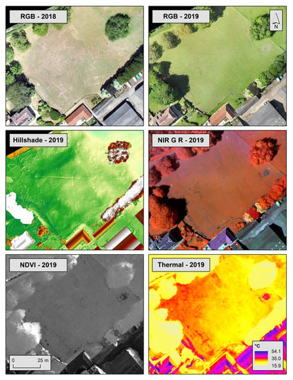
The RGB output from the first survey (July 2018) and the RGB, multispectral, and thermal outputs from the second survey (May 2019) are summarized in Figure 13. In the first survey, as expected, the extremely dry pre-flight conditions that had resulted in visible parch marks on the grass produced an RGB image with excellent contrast between very dry areas and those retaining more moisture. Where buried masonry is present, the mean pixel values in all three bands (R,G,B) are higher than the mean pixel values for the background grass in the field (Table 4). From this lighter appearance in the imagery the outline of one of the priory church’s walls, an anomalous circular feature (possibly a later 17th century Civil War construction), the position of the priory West Range, and a building on the south of the site can all clearly be discerned and their locations were enhanced using Wallis filtration (Equation (9); Figure 14). This local image transform ensures that the standard deviations and means of the image at different locations are approximately equal, which produces excellent local contrast throughout the image, while reducing the overall contrast between bright and dark areas [113] (Figure 14 and Figure 15).
The RGB data acquired during the second survey revealed little archaeological information, most likely as the ground water content was near normal with no extreme dry or wet periods of weather preceding the survey, thus suppressing any visual contrast due to differential vegetation growth [114].
In the hillshade view derived from the RGB imagery, two linear anomalies are prominent and relate to comparatively recent water pipe trenches; these can also be detected, albeit less clearly, in the majority of the other imagery. The hillshade view also clearly reveals depressions and elevated areas that are associated with the archaeological features seen in the RGB imagery from the first survey. The elevated areas may be interpreted as a slight build-up of earth over buried walls, but they are hard to discern from normal RGB aerial imagery or from the ground. However, the parch marks in survey 1 appear to lie mainly in areas of depression where historic robbing of the walls following ruination of the priory has in all probability resulted in a slight lowering of the mean surface level.
Visual assessment of the multispectral imagery, and the derived NDVI, reveal the southern part of the west range with considerable clarity and some of the other features, visible as parch marks during dry conditions in the RGB data for the first survey, are visible to some extent (Figure 13). The contrast in the appearance of the grass above the masonry walls is most likely due to variation in chlorophyll displaying differential reflectance in the red and near-infrared wavelengths [115,116]. Thus, vegetation above masonry walls which is adversely affected by lower water availability, and therefore may contain less chlorophyll, is revealed in the multispectral data with far greater clarity than in the RGB region alone.
The thermal data yield similar information to the multispectral data but provide some increased clarity of the priory church outline. The correction test for topography in the thermal data was not required in this instance, as the site is approximately of uniform height and has no significant slope. The majority of the apparent archaeological features all present with higher temperature values (Table 5) which may be interpreted as differential thermal heat transport in the stone walls [117,118] known to lie below the field surface. However, only two very short sections of opposing walls in the apparent building to the south of the site are faintly revealed in the thermal data, and the remainder of the walls are not discernible.
As the multispectral data appear to yield the greatest level of apparent archaeological information, the data acquired by the Canon S110 camera were processed using the Random Forest classifier to determine if greater clarity could be achieved. Although the multispectral data collected by the Sequoia sensor are more spectrally discrete (Figure 3), the NDVI derived from the data acquired by the Canon camera appeared to show a greater number of features. The difference in the number of features visible between the two sensors may in part be due to the higher spatial resolution of the Canon camera and also due to the fact that the Canon sensor collects information further into the NIR part of the spectrum (wavelengths over 1000 nm) than the Sequoia sensor (limited to 810 nm; Figure 3). The classified data from survey 2 (Figure 16) highlight anomalies that appear to be archaeological in form, and Figure 17 gives an archaeological interpretation of the main features.
The apparent building to the south that is visible in parch marks in July 2018 was not identified as clearly in the thermal data nor in Random Forest classification of the multispectral data collected in May 2019. It is possible that these walls are buried deeper than the building in the west range, and that the trees (over 10 m in height) located between 4 – 18 m directly south east, provide a level of shielding from solar radiation that both reduces the level of absorption of heat and result in a lower differential effect on the surface vegetation chlorophyll.
4. Conclusions
From the first survey of Camp Hill (June 2018), the RGB and multispectral imagery provide little detailed information on the potential archaeology of the site. However, the thermal imagery has revealed, in considerable detail, many features that appear to be man-made and which relate to the former use of the site as a defensible hillfort and enclosure. In addition, the line of the later Roman road is very clearly delineated. The second survey (October 2018) provided less information, with considerably lower contrast between features and background in the thermal data, which is thought to be caused by a combination of the reduced atmospheric temperature and lower solar energy at the time of the autumn survey compared to the summer survey along with the absence of crop cover. The data from the summer survey is by far the most detailed picture of the site yet produced and should lead to further interpretation if the site is investigated by invasive means in the future.
At Shelford Priory, all methods of survey employed—RGB, multispectral, and thermal imaging—have produced useful results, revealing apparent buried archaeology to varying degrees. However, unlike the survey at Camp Hill, the most useful technique at Shelford Priory was found to be multispectral imaging, coupled with Random Forest classification. As before, the results will be exceptionally useful should excavation take place on the site in future, and even without invasive examination, the imagery and classifications appear to provide sufficient information for a provisional ground plan of the priory to be reconstructed.
The key finding of the two survey methodologies is that no single technique is sufficient to attempt to reveal the maximum amount of potential information [119] and that for archaeological survey work a minimum of RGB, multispectral, and thermal imaging should be employed whenever possible. The addition of hyperspectral imagery and UAV acquired LiDAR, which were not available for this study, have considerable potential based on the findings presented here. For precise geographical alignment of survey data, a multisensor ground control target is possible for application with RGB imagery and for multispectral data from Canon S110 and Sequoia sensors, but for thermal image acquisition and processing a separate target made from aluminum foil is suggested.
Author Contributions
Conceptualization, C.B. and B.C.; Methodology, B.C.; Software, C.B. and B.C.; Validation, C.B. and B.C.; Formal Analysis, C.B. and B.C.; Investigation, C.B. and B.C.; Resources, B.C.; Data Curation, C.B. and B.C.; Writing-Original Draft Preparation, C.B. and B.C.; Writing-Review & Editing, C.B. and B.C.; Visualization, C.B. and B.C.; Supervision, C.B. and B.C.; Project Administration, C.B. and B.C.; Funding Acquisition, n/a. All authors have read and agreed to the published version of the manuscript.
Funding
This research received no external funding.
Acknowledgments
The authors wish to acknowledge the kind help and permission for access given by Tony and Helen Strawson at Camp Hill, and by John and Jo Chatterton at Shelford Priory. Thanks are also due to Nicholas Midgley for assistance with surveys at Camp Hill in June 2018.
Conflicts of Interest
The authors declare no conflict of interest.
References
- Rowlands, A.; Sarris, A. Detection of exposed and subsurface archaeological remains using multi-sensor remote sensing. J. Archaeol. Sci. 2007, 34, 795–803. [Google Scholar] [CrossRef]
- Poirier, N.; Hautefeuille, F.; Calastrenc, C. Low Altitude Thermal Survey by Means of an Automated Unmanned Aerial Vehicle for the Detection of Archaeological Buried Structures: Thermal Archaeological Survey by Automated Unmanned Aerial Vehicle. Archaeol. Prospect. 2013, 20, 303–307. [Google Scholar] [CrossRef] [Green Version]
- Kincey, M.; Batty, L.; Chapman, H.; Gearey, B.; Ainsworth, S.; Challis, K. Assessing the changing condition of industrial archaeological remains on Alston Moor, UK, using multisensor remote sensing. J. Archaeol. Sci. 2014, 45, 36–51. [Google Scholar] [CrossRef] [Green Version]
- Agapiou, A.; Lysandrou, V. Remote sensing archaeology: Tracking and mapping evolution in European scientific literature from 1999 to 2015. J. Archaeol. Sci. Rep. 2015, 4, 192–200. [Google Scholar] [CrossRef]
- McLeester, M.; Casana, J.; Schurr, M.R.; Hill, A.C.; Wheeler, J.H. Detecting prehistoric landscape features using thermal, multispectral, and historical imagery analysis at Midewin National Tallgrass Prairie, Illinois. J. Archaeol. Sci. Rep. 2018, 21, 450–459. [Google Scholar] [CrossRef]
- Monterroso Checa, A.; Martínez Reche, T. COSMO SkyMed X-Band SAR application - combined with thermal and RGB images—in the archaeological landscape of Roman Mellaria (Fuente Obejuna-Córdoba, Spain). Archaeol. Prospect. 2018, 25, 301–314. [Google Scholar] [CrossRef]
- Parisi, E.I.; Suma, M.; Güleç Korumaz, A.; Rosina, E.; Tucci, G. Aerial platforms (UAV) surveys in the VIS and TIR range. Applications on archaeology and agriculture. Int. Arch. Photogramm. Remote Sens. Spatial Inf. Sci. 2019, XLII-2/W11, 945–952. [Google Scholar] [CrossRef] [Green Version]
- Šedina, J.; Housarová, E.; Raeva, P. Using RPAS for the detection of archaeological objects using multispectral and thermal imaging. Eur. J. Remote Sens. 2019, 52, 182–191. [Google Scholar] [CrossRef] [Green Version]
- Santos, M.; Disney, M.; Chave, J. Detecting Human Presence and Influence on Neotropical Forests with Remote Sensing. Remote Sens. 2018, 10, 1593. [Google Scholar] [CrossRef] [Green Version]
- Tapete, D. Earth Observation, Remote Sensing, and Geoscientific Ground Investigations for Archaeological and Heritage Research. Geosciences 2019, 9, 161. [Google Scholar] [CrossRef] [Green Version]
- Collis, J. The European Iron Age; Blackwell: London, UK, 1984; ISBN 978-0-415-15139-9. [Google Scholar]
- Rooke, H. Roman Road and Camps. Archaeologia 1789, 9, 196–205. [Google Scholar]
- Watkin, W.T. Roman Nottinghamshire. Archaeol. J. 1886, 43, 11–44. [Google Scholar] [CrossRef]
- Simmons, B.B. Iron Age Hillforts in Nottinghamshire. Trans. Thoroton Soc. 1963, LXVII, 9–20. [Google Scholar]
- Tylecote, R.F. The Prehistory of Metallurgy in the British Isles; Routledge: Oxon, UK, 1986; ISBN 978-0-901-46296-1. [Google Scholar]
- Page, W. The Victoria History of the Counties of England: A History of Nottinghamshire; Constable & Co. Ltd.: London, UK, 1910; Volume II. [Google Scholar]
- Knowles, D.; Hadcock, R.N. Medieval Religious Houses, England and Wales, 2nd ed.; Longman: London, UK, 1972; ISBN 978-0-582-11230-8. [Google Scholar]
- Hamilton, J.; Marcombe, D. Sanctity and Scandal: The medieval Religious Houses of Nottinghamshire; Continuing Education Press: Nottingham, UK, 1998; ISBN 978-1-85041-088-1. [Google Scholar]
- Hartwell, C.; Williamson, E.; Pevsner, N. Nottinghamshire, 3rd ed.; Yale University Press: New Haven, CT, USA, 2020. [Google Scholar]
- Pollard, T.; Oliver, N. Two Men in a Trench: Battlefield Archaeology—The Key to Unlocking the Past; Michael Joseph: London, UK, 2002; ISBN 978-0-7181-4474-6. [Google Scholar]
- Riley, D.N. Air Photography and Archaeology; Duckworth: London, UK, 1987; ISBN 978-0-7156-2101-1. [Google Scholar]
- Barber, M. A History of Aerial Photography and Archaeology: Mata Hari’s Glass Eye and Other Stories; English Heritage: Swindon, UK, 2011; ISBN 978-1-84802-036-8. [Google Scholar]
- Hanson, W.S.; Oltean, I.A. Archaeology from Historical Aerial and Satellite Archives; Springer: New York, NY, USA, 2013; ISBN 978-1-4614-4504-3. [Google Scholar]
- Casana, J.; Kantner, J.; Wiewel, A.; Cothren, J. Archaeological aerial thermography: A case study at the Chaco-era Blue J community, New Mexico. J. Archaeol. Sci. 2014, 45, 207–219. [Google Scholar] [CrossRef]
- Rajani, M.B.; Kasturirangan, K. Multispectral Remote Sensing Data Analysis and Application for Detecting Moats Around Medieval Settlements in South India. J. Indian Soc. Remote Sens. 2014, 42, 651–657. [Google Scholar] [CrossRef]
- Verhoeven, G.; Sevara, C. Trying to Break New Ground in Aerial Archaeology. Remote Sens. 2016, 8, 918. [Google Scholar] [CrossRef] [Green Version]
- Moriarty, C.; Cowley, D.C.; Wade, T.; Nichol, C.J. Deploying multispectral remote sensing for multi-temporal analysis of archaeological crop stress at Ravenshall, Fife, Scotland. Archaeol. Prospect. 2019, 26, 33–46. [Google Scholar] [CrossRef] [Green Version]
- Deng, L.; Mao, Z.; Li, X.; Hu, Z.; Duan, F.; Yan, Y. UAV-based multispectral remote sensing for precision agriculture: A comparison between different cameras. ISPRS J. Photogramm. Remote Sens. 2018, 146, 124–136. [Google Scholar] [CrossRef]
- Hassan, M.A.; Yang, M.; Rasheed, A.; Yang, G.; Reynolds, M.; Xia, X.; Xiao, Y.; He, Z. A rapid monitoring of NDVI across the wheat growth cycle for grain yield prediction using a multi-spectral UAV platform. Plant Sci. 2019, 282, 95–103. [Google Scholar] [CrossRef]
- Calleja, J.F.; Requejo Pagés, O.; Díaz-Álvarez, N.; Peón, J.; Gutiérrez, N.; Martín-Hernández, E.; Cebada Relea, A.; Rubio Melendi, D.; Fernández Álvarez, P. Detection of buried archaeological remains with the combined use of satellite multispectral data and UAV data. Int. J. Appl. Earth Obs. Geoinf. 2018, 73, 555–573. [Google Scholar] [CrossRef]
- Tucker, C.J. Red and photographic infrared linear combinations for monitoring vegetation. Remote Sens. Environ. 1979, 8, 127–150. [Google Scholar] [CrossRef] [Green Version]
- Duan, T.; Chapman, S.C.; Guo, Y.; Zheng, B. Dynamic monitoring of NDVI in wheat agronomy and breeding trials using an unmanned aerial vehicle. Field Crops Res. 2017, 210, 71–80. [Google Scholar] [CrossRef]
- Mondal, A.; Khare, D.; Kundu, S. Identification of Crop Types with the Fuzzy Supervised Classification Using AWiFS and LISS-III Images. In Environment and Earth Observation; Hazra, S., Mukhopadhyay, A., Ghosh, A.R., Mitra, D., Dadhwal, V.K., Eds.; Springer International Publishing: Cham, Switzerland, 2017; pp. 73–86. ISBN 978-3-319-46008-6. [Google Scholar]
- Lupi, S. Fundamentals of Electroheat; Springer International Publishing: Cham, Switzerland, 2017; ISBN 978-3-319-46014-7. [Google Scholar]
- Brooke, C. Thermal Imaging for the Archaeological Investigation of Historic Buildings. Remote Sens. 2018, 10, 1401. [Google Scholar] [CrossRef] [Green Version]
- Karwa, R. Heat and Mass Transfer; Springer: Singapore, 2017; ISBN 978-981-10-1556-4. [Google Scholar]
- Kakaç, S.; Yener, Y.; Naveira-Cotta, C.P. Heat Conduction, 5th ed.; CRC Press; Taylor & Francis Group: Boca Raton, FL, USA, 2018; ISBN 978-1-138-94384-1. [Google Scholar]
- Kuznetsov, A.; Melnikova, I.; Pozdnyakov, D.; Seroukhova, O.; Vasilyev, A. Remote Sensing of the Environment and Radiation Transfer; Springer: Berlin, Germany, 2012; ISBN 978-3-642-14898-9. [Google Scholar]
- Donoghue, D.N.M. Remote Sensing. In Handbook of Archaeological Sciences; Brothwell, D.R., Pollard, A.M., Eds.; John Wiley & Sons: Chichester, UK, 2001; pp. 565–574. [Google Scholar]
- Brutsaert, W. Evaporation into the Atmosphere: Theory, History and Applications; Springer: Dordrecht, The Netherlands, 1982; ISBN 978-94-017-1497-6. [Google Scholar]
- Eppelbaum, L.; Kutasov, I.; Pilchin, A. Applied Geothermics; Lecture Notes in Earth System Sciences; Springer: Berlin, Germany, 2014; ISBN 978-3-642-34022-2. [Google Scholar]
- Bergman, T.L.; Lavine, A.S.; Incropera, F.P.; Dewitt, D.P. Fundamentals of Heat and Mass Transfer, 7th ed.; John Wiley & Sons: Jefferson City, MO, USA, 2011; ISBN 978-0-470-50197-9. [Google Scholar]
- Tang, H.; Li, Z.-L. Quantitative Remote Sensing in Thermal Infrared; Springer Remote Sensing/Photogrammetry; Springer: Berlin, Germany, 2014; ISBN 978-3-642-42026-9. [Google Scholar]
- Petropoulos, G.P.; Carlson, T.N.; Griffiths, H.M. Turbulent Fluxes of Heat and Moisture at the Earth’s Land Surface: Importance, Controlling Parameters, and Conventional Measurement Techniques. In Remote Sensing of Energy Fluxes and Soil Moisture Content; Petropoulos, G.P., Albergel, C., Eds.; CRC Press: Boca Raton, FL, USA, 2014; pp. 3–28. ISBN 978-1-4665-0579-7. [Google Scholar]
- Poelchau, H.S.; Baker, D.R.; Hantschel, T.; Horsfield, B.; Wygrala, B. Basin Simulation and the Design of the Conceptual Basin Model. In Petroleum and Basin Evolution; Welte, D.H., Horsfield, B., Baker, D.R., Eds.; Springer: Berlin, Germany, 1997; pp. 3–70. ISBN 978-3-540-61128-8. [Google Scholar]
- Barry-Macaulay, D.; Bouazza, A.; Singh, R.M.; Wang, B.; Ranjith, P.G. Thermal conductivity of soils and rocks from the Melbourne (Australia) region. Eng. Geol. 2013, 164, 131–138. [Google Scholar] [CrossRef] [Green Version]
- Zarichnyak, Y.P.; Ramazanova, A.E.; Emirov, S.N. Contribution of thermal radiation in measurements of thermal conductivity of sandstone. Phys. Solid State 2013, 55, 2436–2441. [Google Scholar] [CrossRef]
- Bovesecchi, G.; Coppa, P. Basic Problems in Thermal-Conductivity Measurements of Soils. Int. J. Thermophys. 2013, 34, 1962–1974. [Google Scholar] [CrossRef]
- Barry-Macaulay, D.; Bouazza, A.; Wang, B.; Singh, R.M. Evaluation of soil thermal conductivity models. Can. Geotech. J. 2015, 52, 1892–1900. [Google Scholar] [CrossRef]
- Nikolaev, I.V.; Leong, W.H.; Rosen, M.A. Experimental Investigation of Soil Thermal Conductivity Over a Wide Temperature Range. Int. J. Thermophys. 2013, 34, 1110–1129. [Google Scholar] [CrossRef]
- Tarnawski, V.R.; McCombie, M.L.; Momose, T.; Sakaguchi, I.; Leong, W.H. Thermal Conductivity of Standard Sands. Part III. Full Range of Saturation. Int. J. Thermophys. 2013, 34, 1130–1147. [Google Scholar] [CrossRef]
- Dehghan, B. Thermal conductivity determination of ground by new modified two dimensional analytical models: Study cases. Renew. Energy 2018, 118, 393–401. [Google Scholar] [CrossRef]
- Lasaponara, R.; Masini, N.; Holmgren, R.; Backe Forsberg, Y. Integration of aerial and satellite remote sensing for archaeological investigations: A case study of the Etruscan site of San Giovenale. J. Geophys. Eng. 2012, 9, S26–S39. [Google Scholar] [CrossRef]
- Khesin, B.E.; Eppelbaum, L.V. Near-surface thermal prospecting: Review of processing and Interpretation. Geophysics 1994, 59, 744–752. [Google Scholar] [CrossRef]
- Lachenbruch, A.H. Rapid estimation of the topographic disturbance to superficial thermal gradients. Rev. Geophys. 1968, 6, 365. [Google Scholar] [CrossRef]
- SenseFly. S.O.D.A. Camera User Manual; Revision 1.7; senseFly Parrrot Group: Cheseaux-sur-Lausanne, Switzerland, 2018. [Google Scholar]
- SenseFly. S110 RGB, RE and NIR Camera User Manual; Revision 7; senseFly Parrot Group: Cheseaux-sur-Lausanne, Switzerland, 2017. [Google Scholar]
- Parrot. Parrot Sequoia User guide V1.1 05/2017; Parrot Drones SAS: Paris, France, 2017. [Google Scholar]
- FLIR. Tau 2 Longwave Infrared Thermal Imaging Cameras; FLIR Systems Inc.: Wilsonville, OR, USA, 2014. [Google Scholar]
- SenseFly. ThermoMAP Camera User Manual; Revision 5; senseFly Parrot Group: Cheseaux-sur-Lausanne, Switzerland, 2017. [Google Scholar]
- SenseFly. eMotion 3 User Manual; Revision 1.9; senseFly Parrot Group: Cheseaux-sur-Lausanne, Switzerland, 2018. [Google Scholar]
- Tahar, K.N. An Evaluation on Different Number of Ground Control Points in Unmanned Aerial Vehicle Photogrammetric Block. Int. Arch. Photogramm. Remote Sens. Spatial Inf. Sci. 2013, XL-2/W2, 93–98. [Google Scholar] [CrossRef] [Green Version]
- Mesas-Carrascosa, F.-J.; Torres-Sánchez, J.; Clavero-Rumbao, I.; García-Ferrer, A.; Peña, J.-M.; Borra-Serrano, I.; López-Granados, F. Assessing Optimal Flight Parameters for Generating Accurate Multispectral Orthomosaicks by UAV to Support Site-Specific Crop Management. Remote Sens. 2015, 7, 12793–12814. [Google Scholar] [CrossRef] [Green Version]
- Tonkin, T.; Midgley, N. Ground-Control Networks for Image Based Surface Reconstruction: An Investigation of Optimum Survey Designs Using UAV Derived Imagery and Structure-from-Motion Photogrammetry. Remote Sens. 2016, 8, 786. [Google Scholar] [CrossRef] [Green Version]
- Martínez-Carricondo, P.; Agüera-Vega, F.; Carvajal-Ramírez, F.; Mesas-Carrascosa, F.-J.; García-Ferrer, A.; Pérez-Porras, F.-J. Assessment of UAV-photogrammetric mapping accuracy based on variation of ground control points. Int. J. Appl. Earth Obs. Geoinf. 2018, 72, 1–10. [Google Scholar] [CrossRef]
- Oniga, V.-E.; Breaban, A.-I.; Statescu, F. Determining the Optimum Number of Ground Control Points for Obtaining High Precision Results Based on UAS Images. MDPI Proc. 2018, 2, 352. [Google Scholar] [CrossRef] [Green Version]
- Dou, Z.; Han, Y.; Sheng, W.; Ma, X. A Patch-Based Non-local Means Denoising Method Using Hierarchical Searching. In Advances in Image and Graphics Technologies; Tan, T., Ruan, Q., Wang, S., Ma, H., Di, K., Eds.; Springer: Berlin, Germany, 2015; Volume 525, pp. 72–79. ISBN 978-3-662-47790-8. [Google Scholar]
- Ghosh, S.; Mandal, A.K.; Chaudhury, K.N. Pruned non-local means. IET Image Process. 2017, 11, 317–323. [Google Scholar] [CrossRef] [Green Version]
- Frosio, I.; Kautz, J. Statistical Nearest Neighbors for Image Denoising. IEEE Trans. Image Process. 2019, 28, 723–738. [Google Scholar] [CrossRef]
- Buades, A.; Coll, B.; Morel, J.-M. Non-Local Means Denoising. Image Process. Line 2011, 1, 208–212. [Google Scholar] [CrossRef] [Green Version]
- Li, M.; Xu, Y. Improved Non-local Means Algorithm for Image Deno[i]sing. J. Phys. Conf. Ser. 2019, 1237, 022003. [Google Scholar] [CrossRef]
- Bergamaschi, A.; Medjoubi, K.; Messaoudi, C.; Marco, S.; Somogyi, A. MMX-I: Data-processing software for multimodal X-ray imaging and tomography. J. Synchrotron Rad. 2016, 23, 783–794. [Google Scholar] [CrossRef] [PubMed] [Green Version]
- Aggarwal, C.C. Applications of Outlier Analysis. In Outlier Analysis; Springer International Publishing: Cham, Switzerland, 2017; pp. 399–422. ISBN 978-3-319-47577-6. [Google Scholar]
- Tan, D. Image Enhancement Based on Adaptive Median Filter and Wallis Filter. In Proceedings of the 2015 4th National Conference on Electrical, Electronics and Computer Engineering, Xi’an, China, 12–13 December 2015; Atlantis Press: Xi’an, China, 2016; pp. 767–772. [Google Scholar]
- Wang, L.; Wang, A.; Civil Aviation University of China. Research Base of Especial Ground Equipment on Aviation, Tianjin, China. Virtual Texture with Wallis Filter for Terrain Visualization. J. Eng. Sci. Technol. Rev. 2013, 6, 110–114. [Google Scholar] [CrossRef]
- Gaiani, M.; Remondino, F.; Apollonio, F.; Ballabeni, A. An Advanced Pre-Processing Pipeline to Improve Automated Photogrammetric Reconstructions of Architectural Scenes. Remote Sens. 2016, 8, 178. [Google Scholar] [CrossRef] [Green Version]
- Richards, J.A. Clustering and Unsupervised Classification. In Remote Sensing Digital Image Analysis; Springer: Berlin, Germany, 2013; pp. 319–341. ISBN 978-3-642-30061-5. [Google Scholar]
- He, J.; Kim, C.-S.; Kuo, C.-C.J. Interactive Image Segmentation Techniques. In Interactive Segmentation Techniques; Springer: Singapore, 2014; pp. 17–62. ISBN 978-981-4451-59-8. [Google Scholar]
- Pestunov, I.A.; Rylov, S.A.; Berikov, V.B. Hierarchical clustering algorithms for segmentation of multispectral images. Optoelectron. Instrum. Proc. 2015, 51, 329–338. [Google Scholar] [CrossRef]
- Randrianasoa, J.F.; Kurtz, C.; Desjardin, É.; Passat, N. Multi-image Segmentation: A Collaborative Approach Based on Binary Partition Trees. In Mathematical Morphology and Its Applications to Signal and Image Processing; Benediktsson, J.A., Chanussot, J., Najman, L., Talbot, H., Eds.; Springer International Publishing: Cham, Switzerland, 2015; Volume 9082, pp. 253–264. ISBN 978-3-319-18719-8. [Google Scholar]
- Peters, J.F. Watershed, Smirnov Measure, Fuzzy Proximity and Sorted Near Sets. In Computational Proximity; Springer International Publishing: Cham, Switzerland, 2016; Volume 102, pp. 259–290. ISBN 978-3-319-30260-7. [Google Scholar]
- Breiman, L. Random Forests. Mach. Learn. 2001, 45, 5–32. [Google Scholar] [CrossRef] [Green Version]
- Criminisi, A. Decision Forests: A Unified Framework for Classification, Regression, Density Estimation, Manifold Learning and Semi-Supervised Learning. FNT Comput. Graph. Vis. 2011, 7, 81–227. [Google Scholar] [CrossRef]
- Murphy, K.P. Machine Learning: A Probabilistic Perspective; Adaptive computation and machine learning series; MIT Press: Cambridge, MA, USA, 2012; ISBN 978-0-262-01802-9. [Google Scholar]
- Gibril, M.B.A.; Idrees, M.O.; Yao, K.; Shafri, H.Z.M. Integrative image segmentation optimization and machine learning approach for high quality land-use and land-cover mapping using multisource remote sensing data. J. Appl. Remote Sens. 2018, 12, 1. [Google Scholar] [CrossRef]
- Belgiu, M.; Drăguţ, L. Random forest in remote sensing: A review of applications and future directions. ISPRS J. Photogramm. Remote Sens. 2016, 114, 24–31. [Google Scholar] [CrossRef]
- Thanh Noi, P.; Kappas, M. Comparison of Random Forest, k-Nearest Neighbor, and Support Vector Machine Classifiers for Land Cover Classification Using Sentinel-2 Imagery. Sensors 2017, 18, 18. [Google Scholar] [CrossRef] [PubMed] [Green Version]
- Avand, M.; Janizadeh, S.; Naghibi, S.A.; Pourghasemi, H.R.; Khosrobeigi Bozchaloei, S.; Blaschke, T. A Comparative Assessment of Random Forest and k-Nearest Neighbor Classifiers for Gully Erosion Susceptibility Mapping. Water 2019, 11, 2076. [Google Scholar] [CrossRef] [Green Version]
- Rogers, J.; Gunn, S. Identifying Feature Relevance Using a Random Forest. In Subspace, Latent Structure and Feature Selection; Springer: Bohinj, Slovenia, 2006; pp. 173–184. [Google Scholar]
- Millard, K.; Richardson, M. On the Importance of Training Data Sample Selection in Random Forest Image Classification: A Case Study in Peatland Ecosystem Mapping. Remote Sens. 2015, 7, 8489–8515. [Google Scholar] [CrossRef] [Green Version]
- Fornaser, A.; De Cecco, M.; Bosetti, P.; Mizumoto, T.; Yasumoto, K. Sigma-Z random forest, classification and confidence. Meas. Sci. Technol. 2019, 30, 025002. [Google Scholar] [CrossRef]
- Haubold, C.; Schiegg, M.; Kreshuk, A.; Berg, S.; Koethe, U.; Hamprecht, F.A. Segmenting and Tracking Multiple Dividing Targets Using ilastik. In Focus on Bio-Image Informatics; De Vos, W.H., Munck, S., Timmermans, J.-P., Eds.; Springer International Publishing: Cham, Switzerland, 2016; Volume 219, pp. 199–229. ISBN 978-3-319-28547-4. [Google Scholar]
- Berg, S.; Kutra, D.; Kroeger, T.; Straehle, C.N.; Kausler, B.X.; Haubold, C.; Schiegg, M.; Ales, J.; Beier, T.; Rudy, M.; et al. ilastik: Interactive machine learning for (bio)image analysis. Nat. Methods 2019, 16, 1226–1232. [Google Scholar] [CrossRef]
- Lormand, C.; Zellmer, G.F.; Németh, K.; Kilgour, G.; Mead, S.; Palmer, A.S.; Sakamoto, N.; Yurimoto, H.; Moebis, A. Weka Trainable Segmentation Plugin in ImageJ: A Semi-Automatic Tool Applied to Crystal Size Distributions of Microlites in Volcanic Rocks. Microsc. Microanal. 2018, 24, 667–675. [Google Scholar] [CrossRef]
- Lakshminarayanan, B. Decision Trees and Forests: A Probabilistic Perspective; University College London: London, UK, 2016. [Google Scholar]
- Pinty, B.; Lavergne, T.; Widlowski, J.-L.; Gobron, N.; Verstraete, M.M. On the need to observe vegetation canopies in the near-infrared to estimate visible light absorption. Remote Sens. Environ. 2009, 113, 10–23. [Google Scholar] [CrossRef]
- Garrett, R.H.; Grisham, C.M. Biochemistry, 6th ed.; Cengage Learning: Boston, MA, USA, 2017; ISBN 978-1-305-57720-6. [Google Scholar]
- Clutterbuck, B.; Chico, G.; Labadz, J.; Midgley, N. The Potential of Geospatial Technology for Monitoring Peatland Environments. In Inventory, Value and Restoration of Peatlands and Mires: Recent Contributions; Fernández-García, J.M., Pérez, F.J., Eds.; Provincial Council of Bizkaia: Bilbao, Spain, 2018; pp. 167–181. [Google Scholar]
- Brooke, C. A Historical Account and Survey of Camp Hill, Hexgreave Park, Nottinghamshire. Unpublished Dissertation, University of Cambridge Local Examinations Syndicate, Cambridge, UK, 1975. [Google Scholar]
- Bird, R.B.; Stewart, W.E.; Lightfoot, E.N. Transport Phenomena, Rev. 2nd ed.; Wiley: New York, NY, USA, 2007; ISBN 978-0-470-11539-8. [Google Scholar]
- Fuchs, H.U. The Dynamics of Heat; Graduate Texts in Physics; Springer: New York, NY, USA, 2010; ISBN 978-1-4419-7603-1. [Google Scholar]
- Wallace, L.; Lucieer, A.; Watson, C.; Turner, D. Development of a UAV-LiDAR System with Application to Forest Inventory. Remote Sens. 2012, 4, 1519–1543. [Google Scholar] [CrossRef] [Green Version]
- Campana, S. Drones in Archaeology. State-of-the-art and Future Perspectives: Drones in Archaeology. Archaeol. Prospect. 2017, 24, 275–296. [Google Scholar] [CrossRef]
- Khan, S.; Aragão, L.; Iriarte, J. A UAV–lidar system to map Amazonian rainforest and its ancient landscape transformations. Int. J. Remote Sens. 2017, 38, 2313–2330. [Google Scholar] [CrossRef]
- Risbøl, O.; Gustavsen, L. LiDAR from drones employed for mapping archaeology - Potential, benefits and challenges. Archaeol. Prospect. 2018, 25, 329–338. [Google Scholar] [CrossRef]
- Kullberg, E.G.; DeJonge, K.C.; Chávez, J.L. Evaluation of thermal remote sensing indices to estimate crop evapotranspiration coefficients. Agric. Water Manag. 2017, 179, 64–73. [Google Scholar] [CrossRef] [Green Version]
- Brenner, C.; Zeeman, M.; Bernhardt, M.; Schulz, K. Estimation of evapotranspiration of temperate grassland based on high-resolution thermal and visible range imagery from unmanned aerial systems. Int. J. Remote Sens. 2018, 39, 5141–5174. [Google Scholar] [CrossRef] [PubMed] [Green Version]
- Ramachandran, K.M.; Tsokos, C.P. Mathematical Statistics with Applications in R, 2nd ed.; Elsevier: Oxford, UK, 2015; ISBN 978-0-12-417113-8. [Google Scholar]
- Davino, C.; Vistocco, D. Quantile Regression for Clustering and Modeling Data. In Advances in Statistical Models for Data Analysis; Morlini, I., Minerva, T., Vichi, M., Eds.; Springer International Publishing: Cham, Switzerland, 2015; pp. 85–95. ISBN 978-3-319-17376-4. [Google Scholar]
- Chen, B.; Zhu, Y.; Hu, J.; Principe, J.C. System Identification Under Information Divergence Criteria. In System Parameter Identification; Elsevier: London, UK, 2013; pp. 167–204. ISBN 978-0-12-404574-3. [Google Scholar]
- Denis, D.J. Applied Univariate, Bivariate, and Multivariate Statistics; John Wiley & Sons, Inc: Hoboken, NJ, USA, 2016; ISBN 978-1-118-63223-9. [Google Scholar]
- De Oliveira Ferreira Silva, C.; de Castro Teixeira, A.H.; Manzione, R.L. Agriwater: An R package for spatial modelling of energy balance and actual evapotranspiration using satellite images and agrometeorological data. Environ. Model. Softw. 2019, 120, 104497. [Google Scholar] [CrossRef]
- Fan, C.; Chen, X.; Zhong, L.; Zhou, M.; Shi, Y.; Duan, Y. Improved Wallis Dodging Algorithm for Large-Scale Super-Resolution Reconstruction Remote Sensing Images. Sensors 2017, 17, 623. [Google Scholar] [CrossRef] [Green Version]
- Wilson, D. The Formation and Appearance of Archaeological Soil Marks. In Into the Sun: Essays in Air Photography in Archaeology in Honour of Derrick Riley; University of Sheffield: Sheffield, UK, 1989; pp. 61–71. [Google Scholar]
- Gitelson, A.A.; Merzlyak, M.N. Signature Analysis of Leaf Reflectance Spectra: Algorithm Development for Remote Sensing of Chlorophyll. J. Plant Physiol. 1996, 148, 494–500. [Google Scholar] [CrossRef]
- Askari, M.S.; McCarthy, T.; Magee, A.; Murphy, D.J. Evaluation of Grass Quality under Different Soil Management Scenarios Using Remote Sensing Techniques. Remote Sens. 2019, 11, 1835. [Google Scholar] [CrossRef] [Green Version]
- Jacobs, P.A. Thermal Infrared Characterization of Ground Targets and Backgrounds, 2nd ed.; Tutorial texts in optical engineering; SPIE: Bellingham, Washington, DC, USA, 2006; ISBN 978-0-8194-6082-0. [Google Scholar]
- Škerget, L.; Tadeu, A.; Brebbia, C.A. Transient simulation of coupled heat and moisture flow through a multi-layer porous solid exposed to solar heat flux. Int. J. Heat Mass Transf. 2018, 117, 273–279. [Google Scholar] [CrossRef]
- Agudo, P.; Pajas, J.; Pérez-Cabello, F.; Redón, J.; Lebrón, B. The Potential of Drones and Sensors to Enhance Detection of Archaeological Cropmarks: A Comparative Study Between Multi-Spectral and Thermal Imagery. Drones 2018, 2, 29. [Google Scholar] [CrossRef] [Green Version]
Figure 1.
Location of Camp Hill and Shelford Priory.

Figure 2.
Site conditions at Camp Hill and Shelford Priory as visible in RGB imagery (white crosses show the location of ground control targets when used).
Figure 2.
Site conditions at Camp Hill and Shelford Priory as visible in RGB imagery (white crosses show the location of ground control targets when used).

Figure 3.
Band specifications for multispectral sensors used in this study: (a) Canon Powershot S110 NIR; (b) Parrot Sequoia.
Figure 3.
Band specifications for multispectral sensors used in this study: (a) Canon Powershot S110 NIR; (b) Parrot Sequoia.

Figure 4.
Multisensor target design.

Figure 5.
Appearance of multisensor ground control target in imagery collected by the senseFly Sensor Optimised for Drone Applications (S.O.D.A.), Parrot Sequoia and senseFly thermoMAP at approximately 75 m above elevation data (AED) (Shuttle Radar Topography Mission (SRTM) data).
Figure 5.
Appearance of multisensor ground control target in imagery collected by the senseFly Sensor Optimised for Drone Applications (S.O.D.A.), Parrot Sequoia and senseFly thermoMAP at approximately 75 m above elevation data (AED) (Shuttle Radar Topography Mission (SRTM) data).

Figure 6.
Appearance of multisensor and aluminium foil ground control targets in imagery collected by the senseFly S.O.D.A., Canon Powershot, Parrot Sequoia and senseFly thermoMAP at approximately 75 m AED (SRTM data).
Figure 6.
Appearance of multisensor and aluminium foil ground control targets in imagery collected by the senseFly S.O.D.A., Canon Powershot, Parrot Sequoia and senseFly thermoMAP at approximately 75 m AED (SRTM data).

Figure 7.
Image outputs for Camp Hill in survey 1 (June 2018). Note that the Hillshade view is an effect applied to the digital surface model (DSM) in ArcGIS for visualisation.
Figure 7.
Image outputs for Camp Hill in survey 1 (June 2018). Note that the Hillshade view is an effect applied to the digital surface model (DSM) in ArcGIS for visualisation.

Figure 8.
Image outputs for Camp Hill in survey 2 (October 2018). Note that the Hillshade view is an effect applied to the DSM in ArcGIS for visualisation.
Figure 8.
Image outputs for Camp Hill in survey 2 (October 2018). Note that the Hillshade view is an effect applied to the DSM in ArcGIS for visualisation.

Figure 9.
Interpreted thermal output from survey 1 processed using the Random Forest classifier.

Figure 10.
Range of temperature values recorded in thermal data for both surveys at Camp Hill.

Figure 11.
Camp Hill thermal data: quantile (QQ) plots of survey 1 (a) and survey 2 (b) versus standard normal.
Figure 11.
Camp Hill thermal data: quantile (QQ) plots of survey 1 (a) and survey 2 (b) versus standard normal.

Figure 12.
Camp Hill thermal data: optimum distribution fit for surveys 1 (a) and 2 (b).

Figure 13.
Image outputs for the main complex at Shelford priory (near infra-red (NIR) G R – from Sequoia sensor; normalized difference vegetation index (NDVI) – derived from R and NIR bands from Canon S110 NIR). Note that the Hillshade view is an effect applied to the DSM in ArcGIS for visualisation.

Figure 14.
Detail of the priory area at Shelford from survey 1 (July 2018) with Wallis filtration.

Figure 15.
Effect of using Wallis filtration on the RGB image of Shelford Priory. Two extracted regions of interest (ROIs) across the probable Civil War feature are sectioned, (a) shows the unfiltered raw RGB imagery and (b) shows the Wallis filtered result. The graph compares the signal response across the section line x-y.

Figure 16.
Multispectral output using the Random Forest classifier.

Figure 17.
Interpretation of the main archaeological features based on Random Forest classifier.


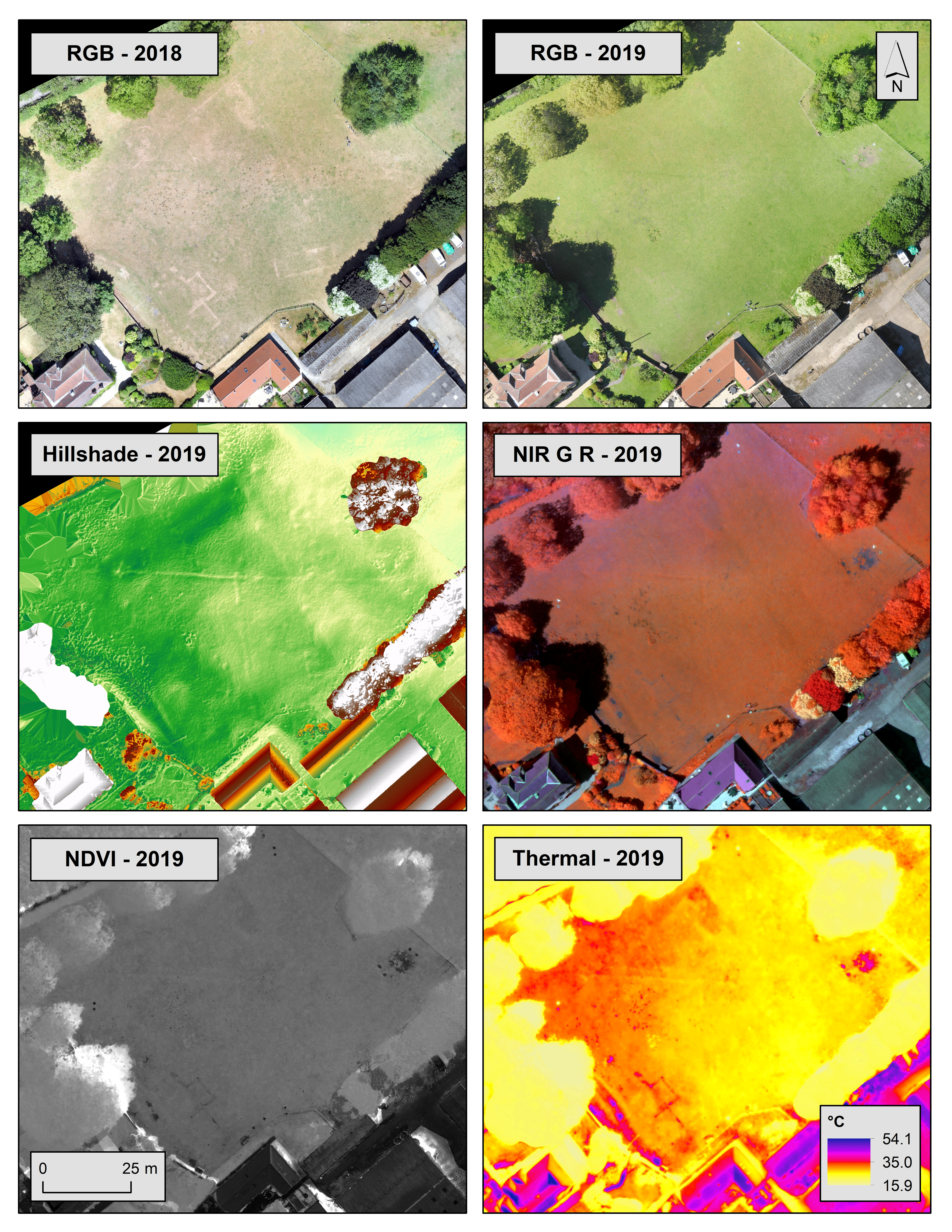
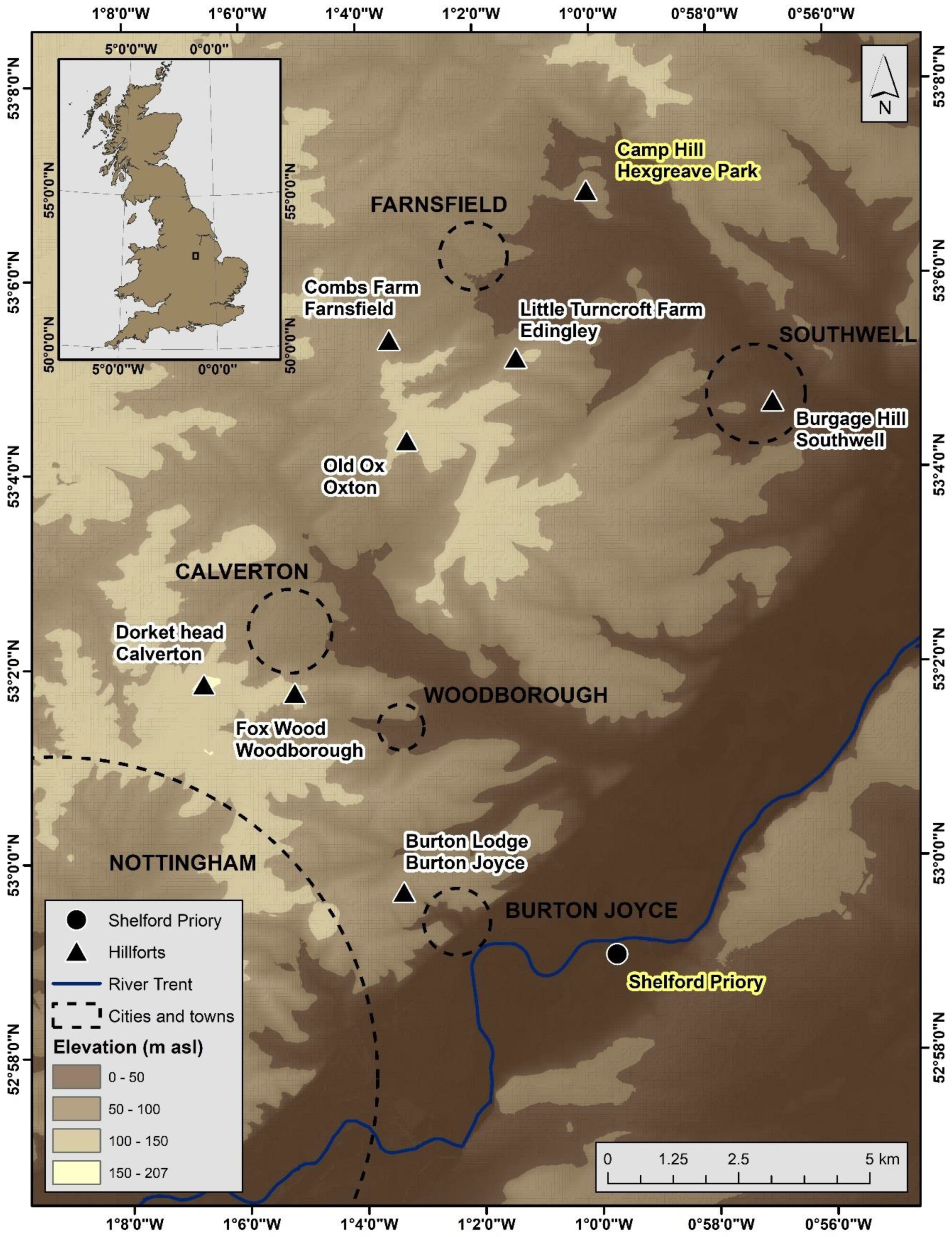
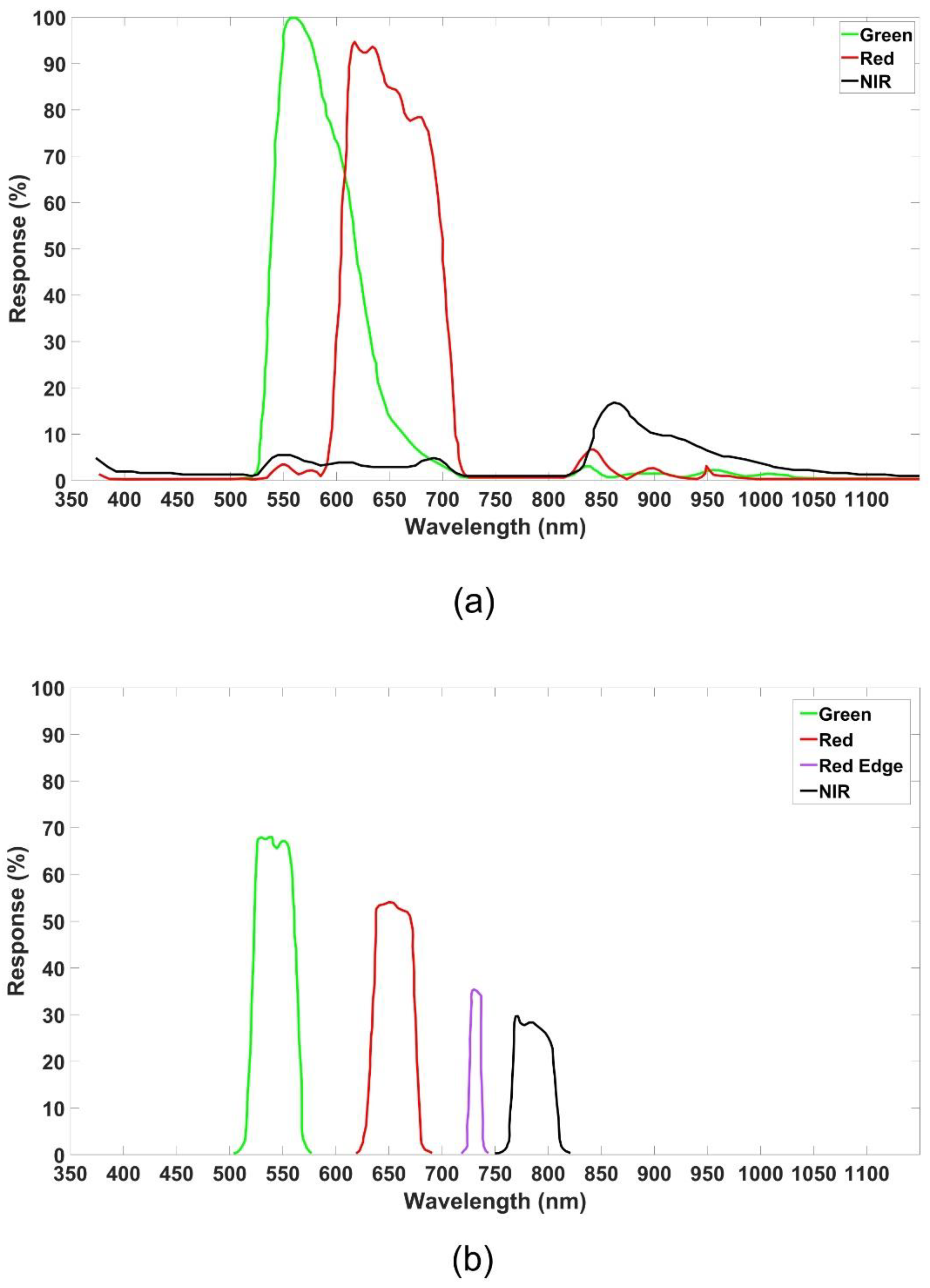
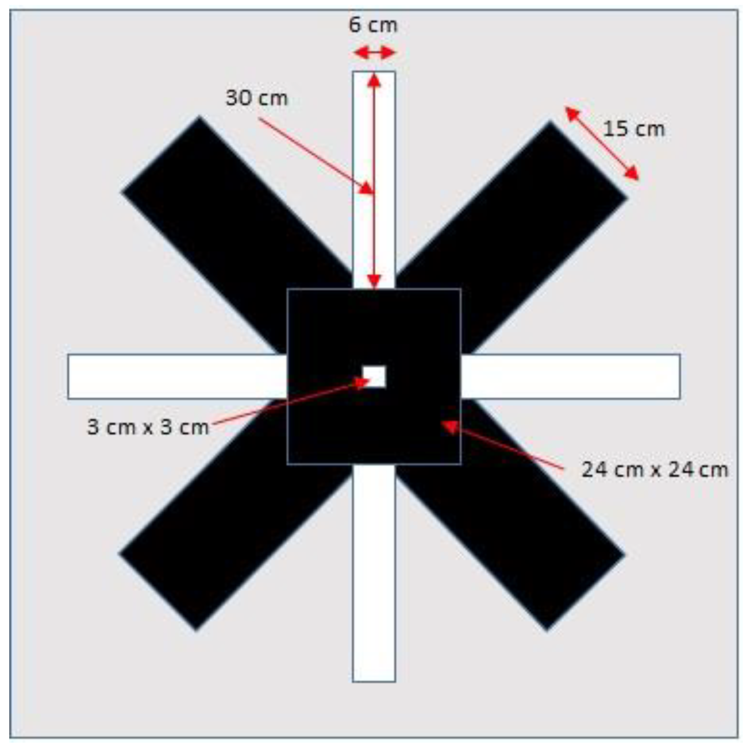
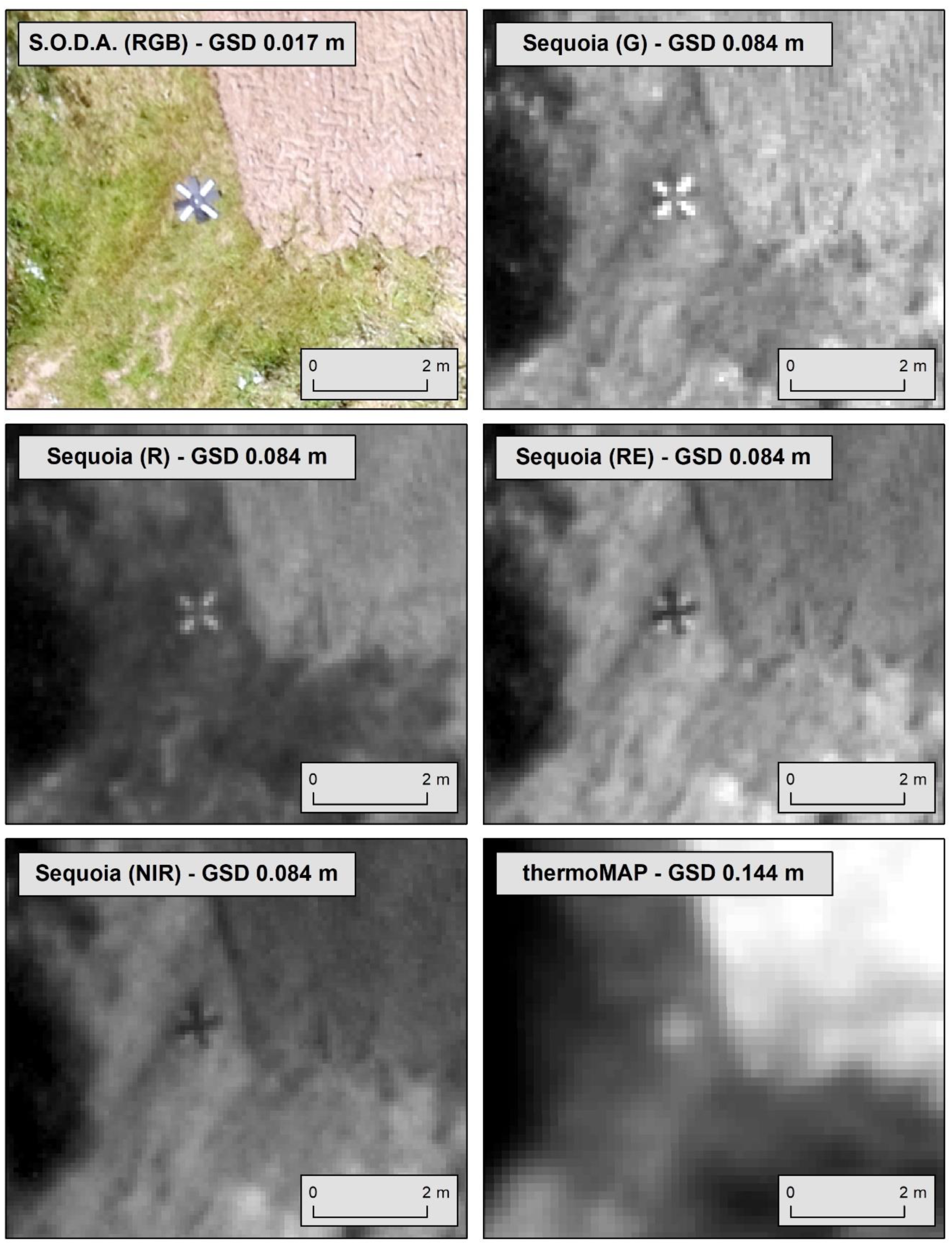
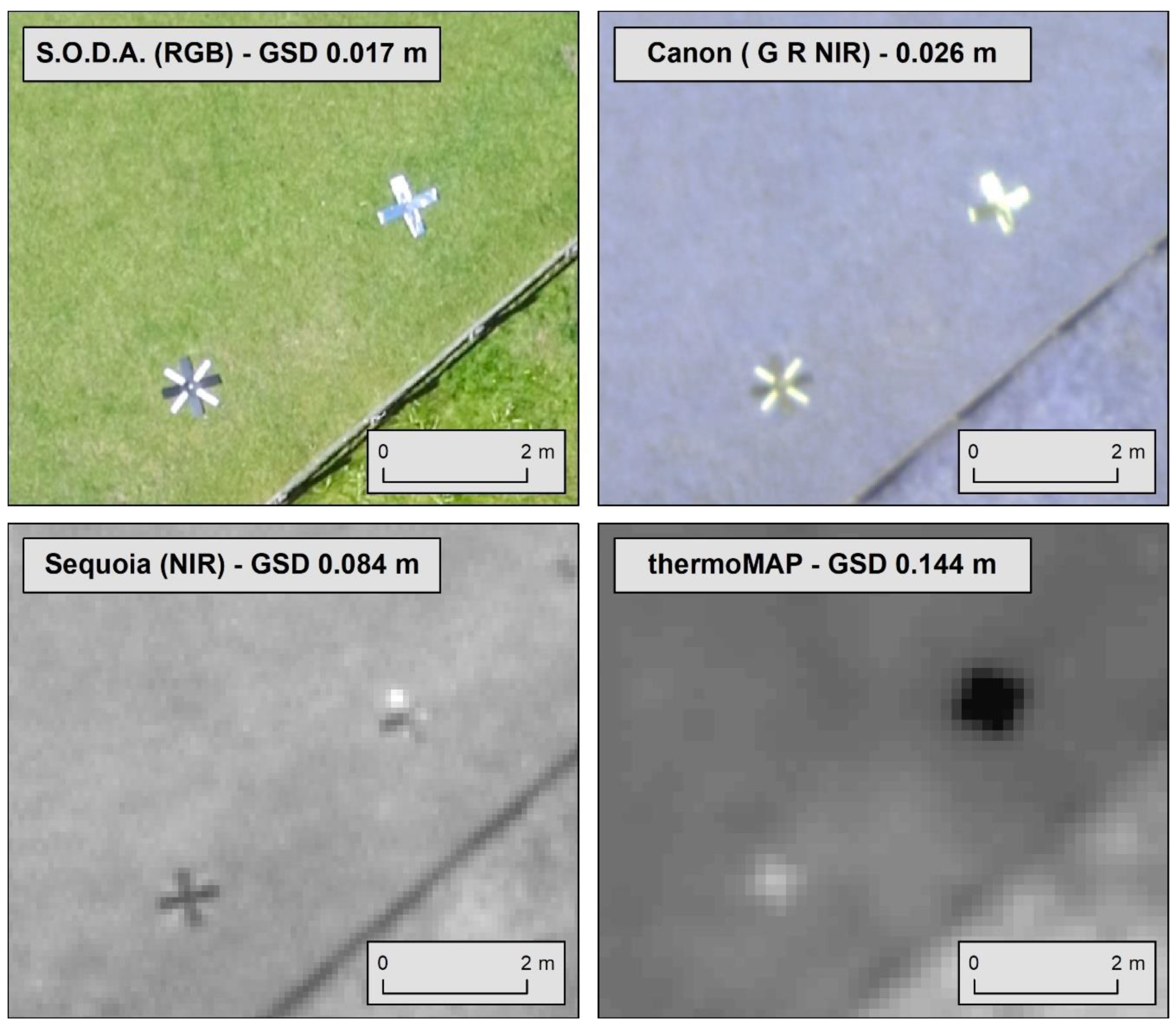
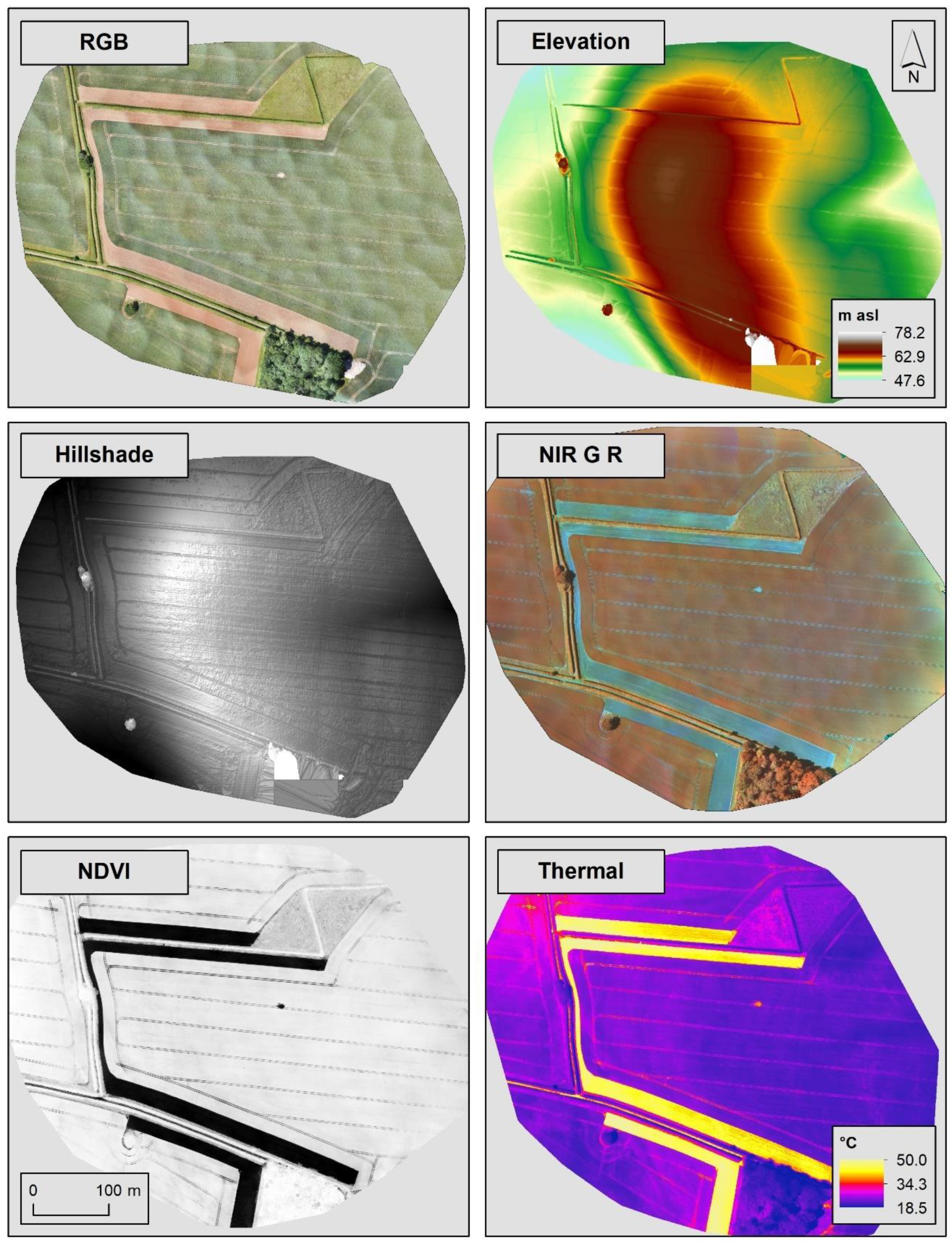
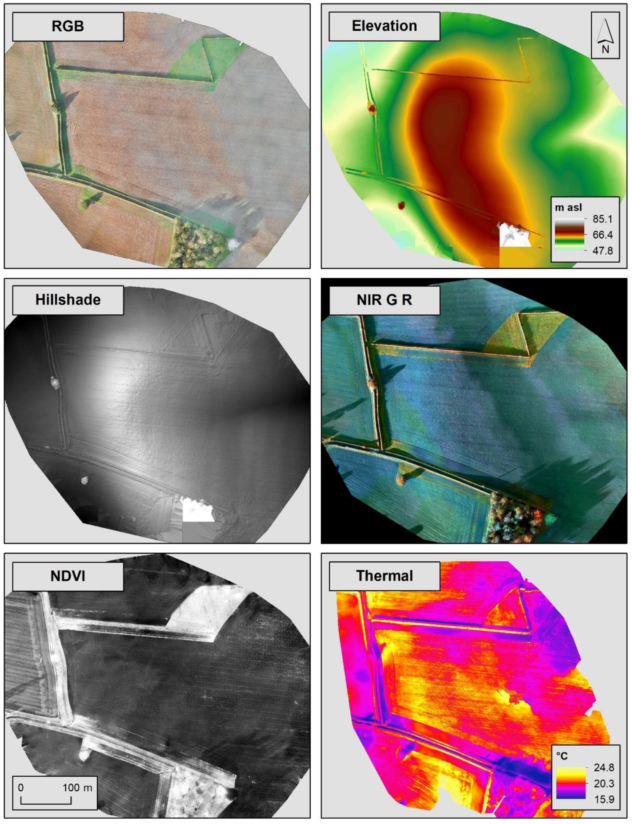
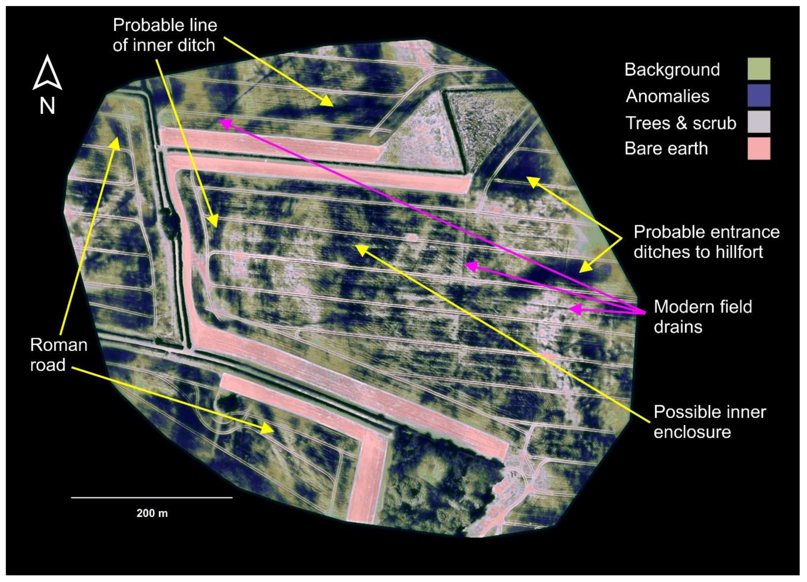
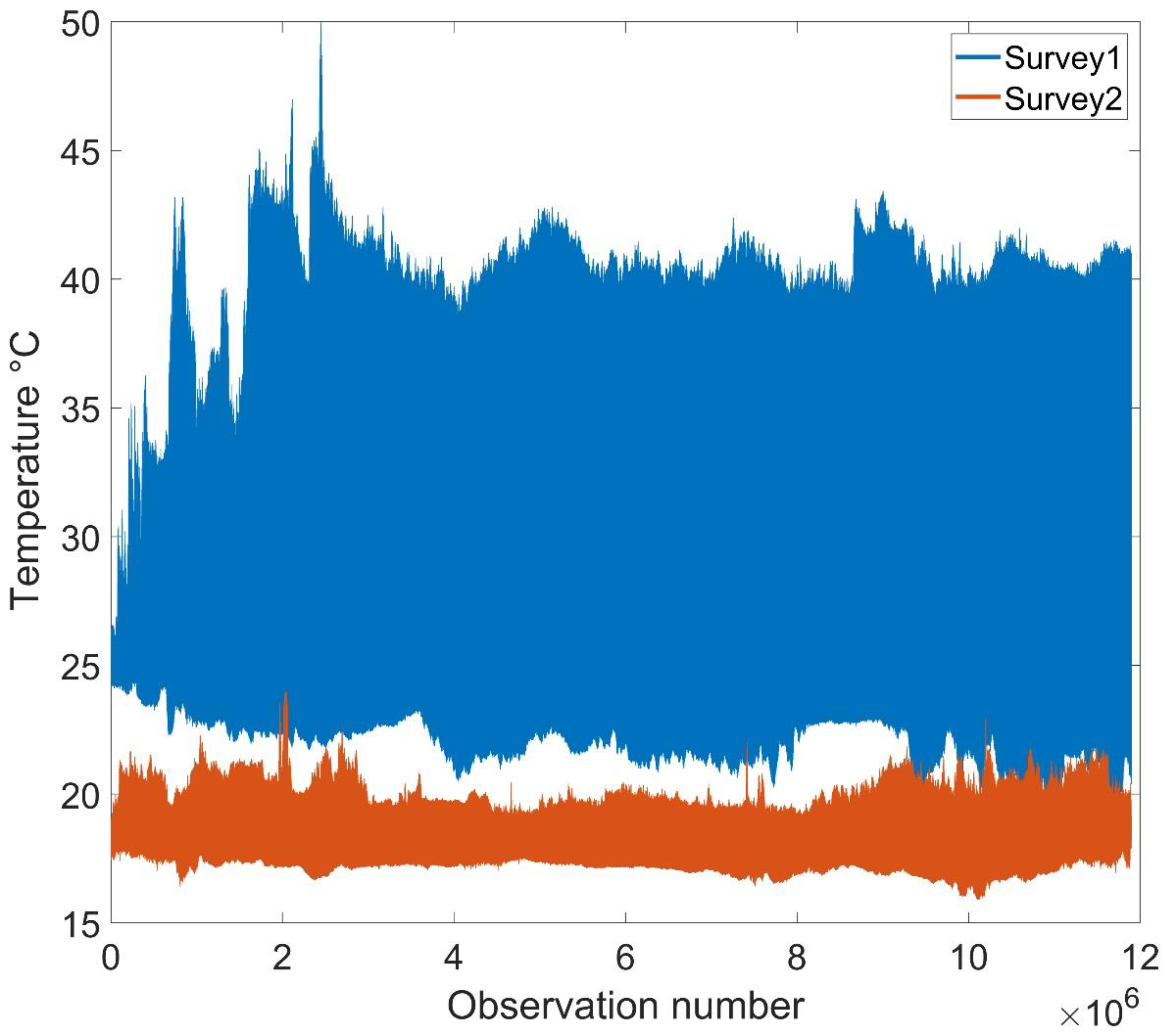
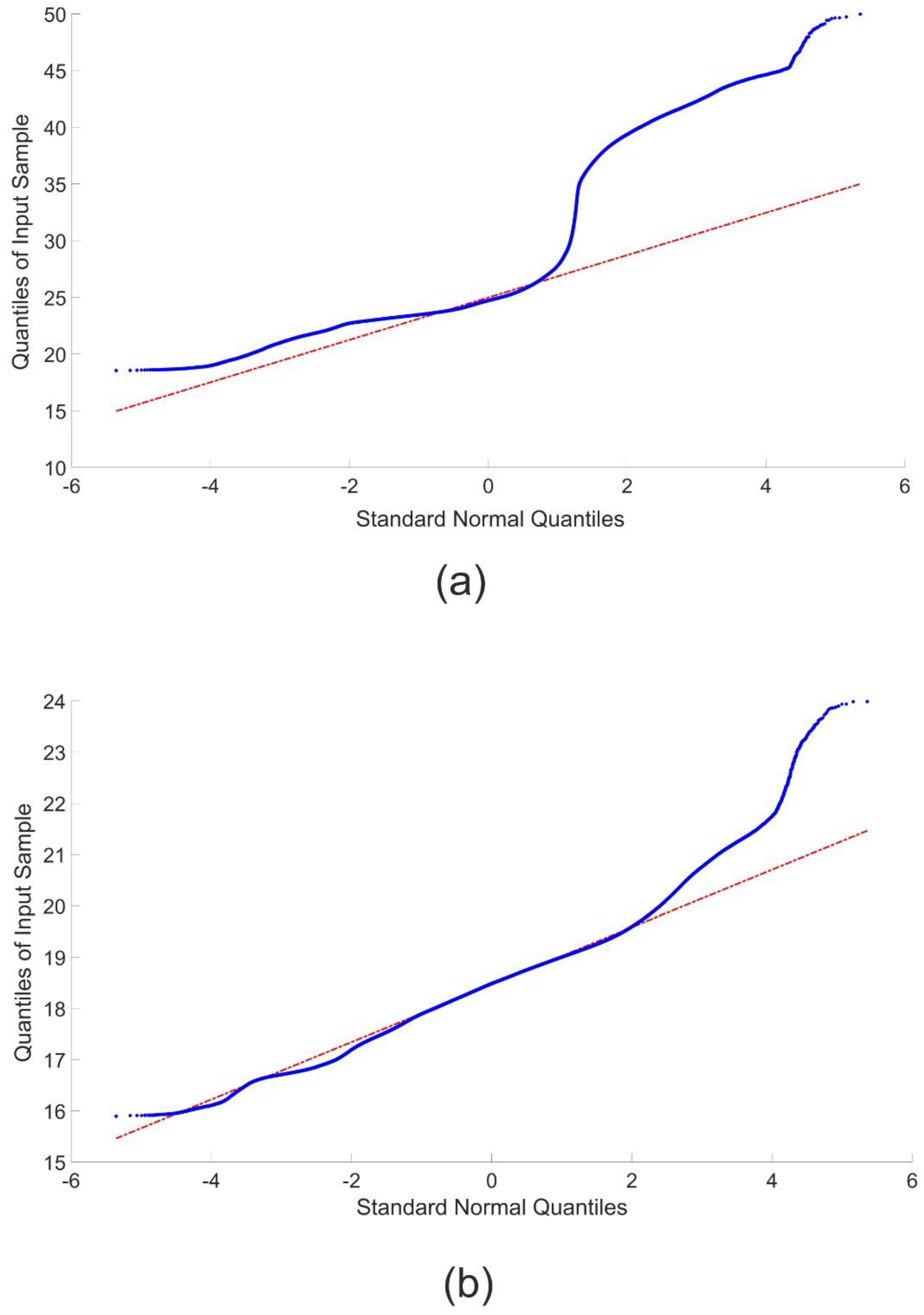
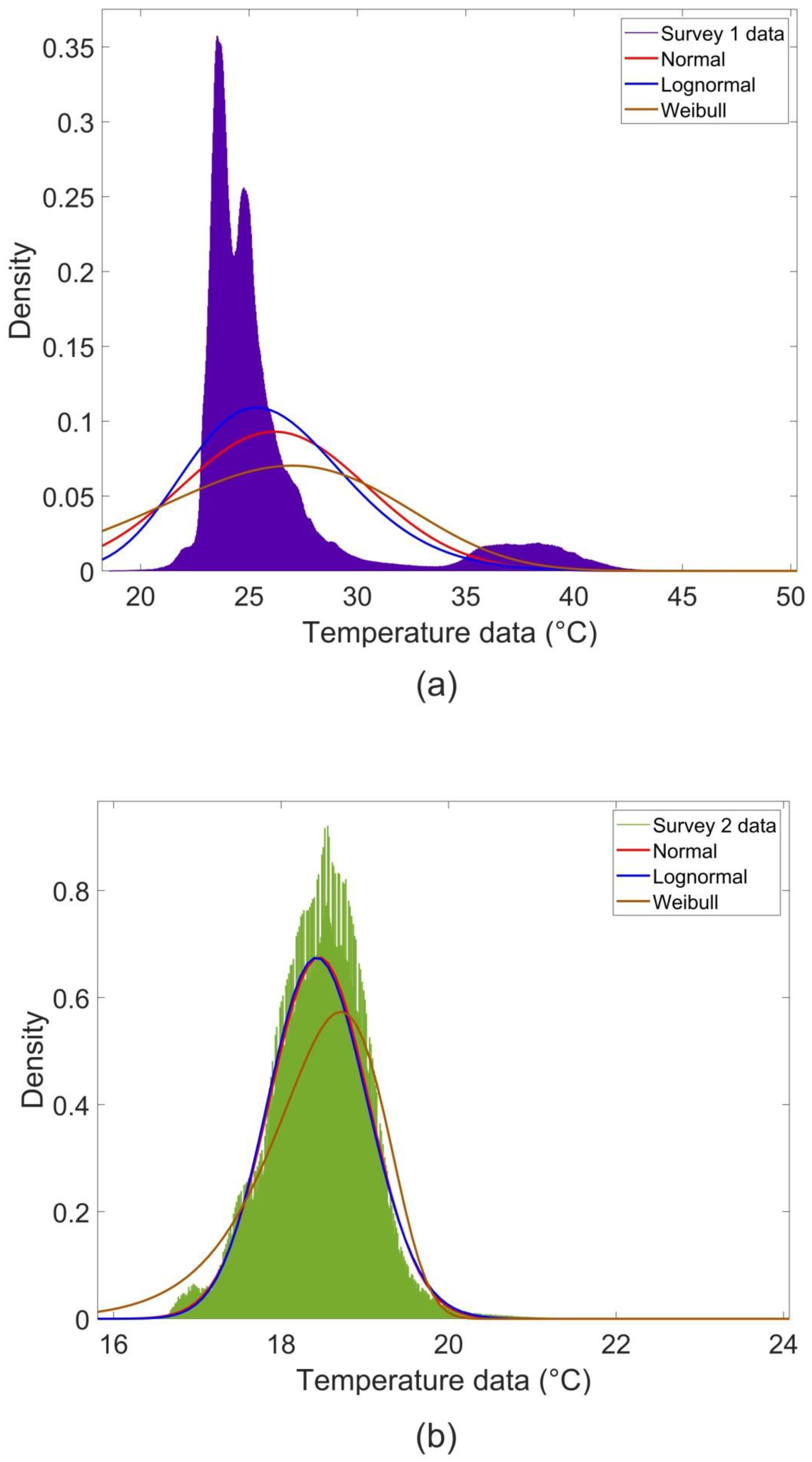
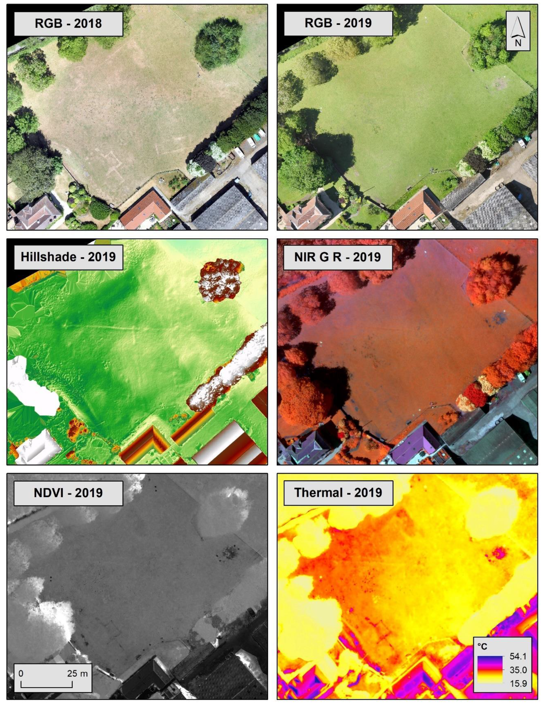
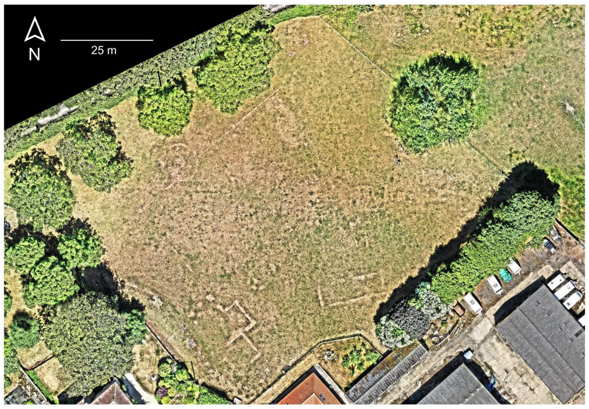
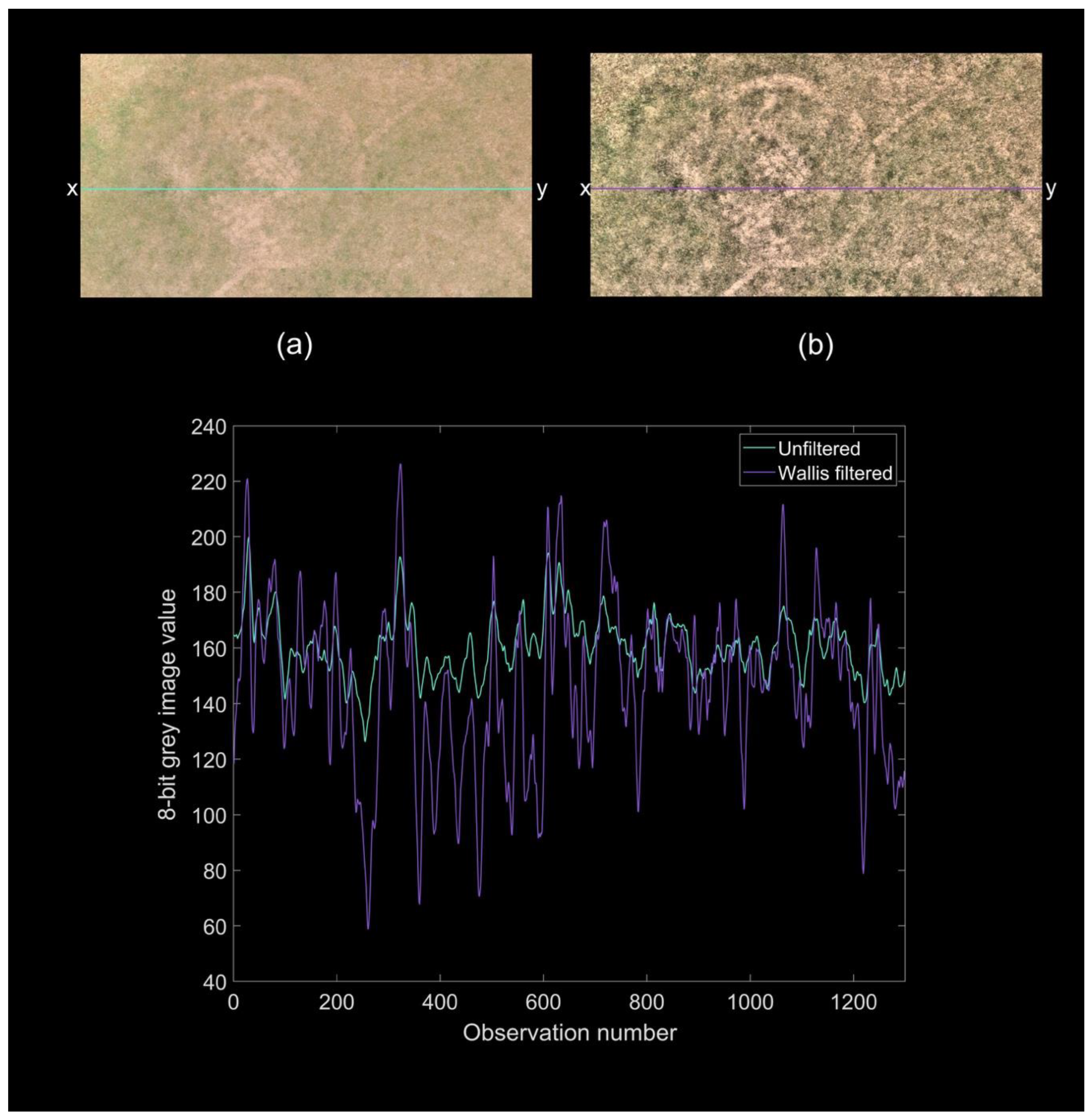
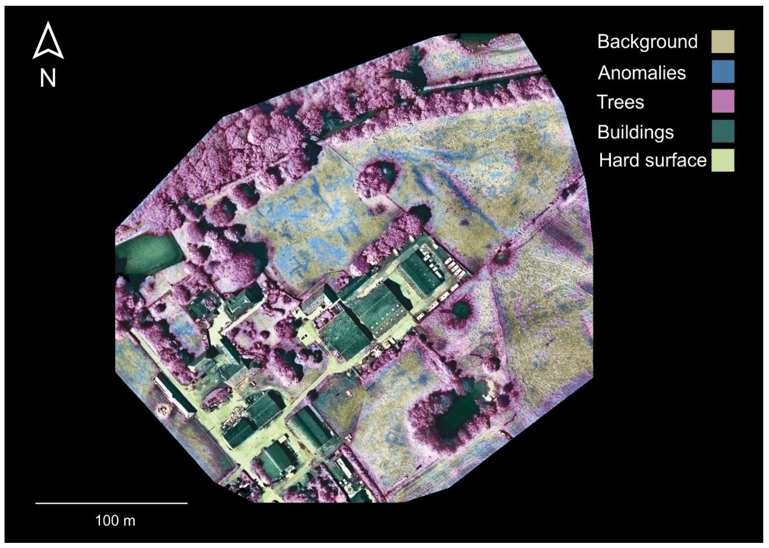
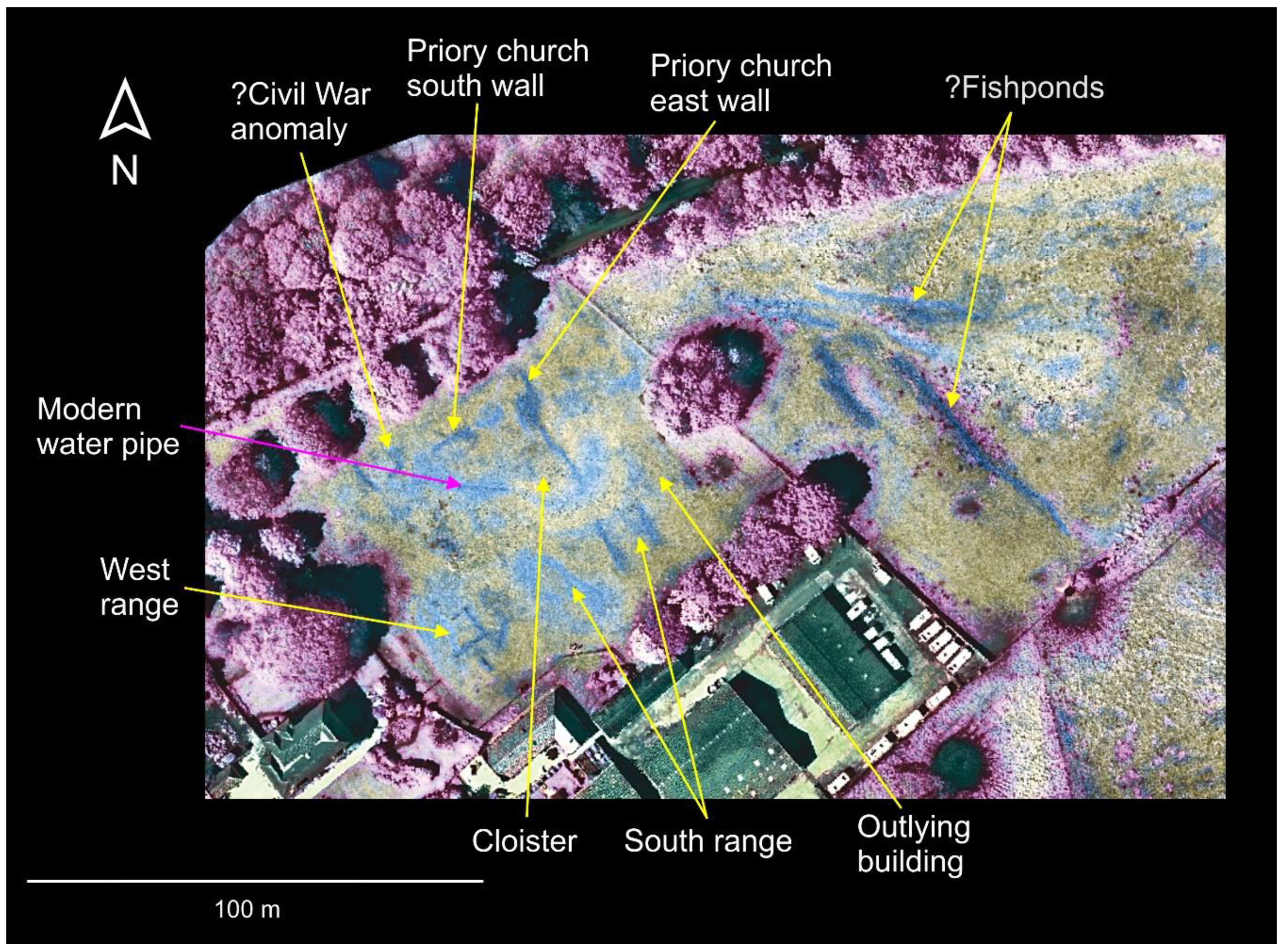
Table 1.
Image Outputs for All Surveys (TM – thermoMAP; * Orthomosaic; n.d. – not Determined; n.a. – not Applicable).
Table 1.
Image Outputs for All Surveys (TM – thermoMAP; * Orthomosaic; n.d. – not Determined; n.a. – not Applicable).
| Survey | Products | Area (ha) | GSD (m) | GCP No. | RMSE X (m) | RMSE Y (m) | RMSE Z (m) | RMSE XYZ (m) |
|---|---|---|---|---|---|---|---|---|
| Camp Hill June 2018 | ||||||||
| SODA | RGB*; DSM | 22.7 | 0.017 | n.a. | n.d. | n.d. | n.d. | n.d. |
| Sequoia | G R RE NIR*; NDVI | 25.0 | 0.084 | n.a. | n.d. | n.d. | n.d. | n.d. |
| TM | Thermal IR*; T (°C) | 24.3 | 0.144 | n.a. | n.d. | n.d. | n.d. | n.d. |
| Camp Hill October 2018 | ||||||||
| SODA | RGB*; DSM | 25.6 | 0.018 | 4 | 0.017 | 0.007 | 0.005 | 0.01 |
| Sequoia | G R RE NIR*; NDVI | 29.1 | 0.081 | 4 | 0.012 | 0.004 | 0.011 | 0.008 |
| TM | Thermal IR*; T (°C) | 21.9 | 0.136 | 4 | n.d. | n.d. | n.d. | n.d. |
| Shelford Priory July 2018 | ||||||||
| SODA | RGB*; DSM | 7.9 | 0.017 | 6 | 0.018 | 0.017 | 0.016 | 0.017 |
| Shelford Priory May 2019 | ||||||||
| SODA | RGB*; DSM | 7.1 | 0.017 | 6 | 0.013 | 0.015 | 0.012 | 0.014 |
| Canon | G R RE NIR*; NDVI | 8.1 | 0.026 | 6 | 0.015 | 0.024 | 0.013 | 0.017 |
| Sequoia | G R RE NIR*; NDVI | 9.0 | 0.083 | 6 | 0.008 | 0.012 | 0.008 | 0.009 |
| TM | Thermal IR*; T (°C) | 11.1 | 0.144 | 4 | 0.047 | 0.116 | 0.117 | 0.087 |
Table 2.
Mean Temperature Values of Background Field, Black Target Material and Aluminium Foil.
| Feature | Mean Temperature (°C) | Standard Deviation |
|---|---|---|
| Background field (grass) | 26.9 | 0.69 |
| Black material | 30.1 | 0.63 |
| Foil | 17.8 | 1.78 |
Table 3.
Regression Coefficients for Topography Correction in the Camp Hill Thermal Data.
| Survey | Coefficient Estimates | Standard Error | t-Statistic | p-Value |
|---|---|---|---|---|
| Camp Hill June 2018 | ||||
| α (intercept) | 22.281 | 0.121 | 184.05 | 0 |
| β (slope) | 0.020 | 0.002 | 9.438 | 7.331e−20 |
| Camp Hill October 2018 | ||||
| α (intercept) | 17.331 | 0.090 | 191.89 | 0 |
| β (slope) | 0.027 | 0.002 | 16.636 | 2.16e−50 |
Table 4.
Mean Pixel Values with Standard Deviations (s.d.) for Each Band in the RGB Data for Shelford in July 2018.
Table 4.
Mean Pixel Values with Standard Deviations (s.d.) for Each Band in the RGB Data for Shelford in July 2018.
| Feature | Red | s.d. | Green | s.d. | Blue | s.d. |
|---|---|---|---|---|---|---|
| Background field | 160.89 | 13.85 | 155.61 | 10.71 | 110.44 | 12.28 |
| Priory wall | 213.03 | 12.24 | 178.09 | 10.38 | 140.47 | 11.84 |
| Circular feature | 210.06 | 9.25 | 175.50 | 8.30 | 146.12 | 8.62 |
| West range | 211.22 | 10.51 | 182.49 | 10.29 | 155.82 | 10.91 |
| Building to south | 209.36 | 16.21 | 185.00 | 15.66 | 151.47 | 18.12 |
Table 5.
Mean Temperature Values for Anomalies Visible at Shelford Priory.
| Feature | Mean Temperature (°C) | Standard Deviation |
|---|---|---|
| Background field | 26.45 | 0.33 |
| Priory wall | 28.10 | 0.37 |
| Circular feature | 30.92 | 0.46 |
| West range | 31.14 | 0.78 |
| Building to south | 26.80 | 0.25 |
© 2019 by the authors. Licensee MDPI, Basel, Switzerland. This article is an open access article distributed under the terms and conditions of the Creative Commons Attribution (CC BY) license (http://creativecommons.org/licenses/by/4.0/).
Share and Cite
MDPI and ACS Style
Brooke, C.; Clutterbuck, B. Mapping Heterogeneous Buried Archaeological Features Using Multisensor Data from Unmanned Aerial Vehicles. Remote Sens. 2020, 12, 41. https://0-doi-org.brum.beds.ac.uk/10.3390/rs12010041
AMA Style
Brooke C, Clutterbuck B. Mapping Heterogeneous Buried Archaeological Features Using Multisensor Data from Unmanned Aerial Vehicles. Remote Sensing. 2020; 12(1):41. https://0-doi-org.brum.beds.ac.uk/10.3390/rs12010041
Chicago/Turabian StyleBrooke, Christopher, and Ben Clutterbuck. 2020. "Mapping Heterogeneous Buried Archaeological Features Using Multisensor Data from Unmanned Aerial Vehicles" Remote Sensing 12, no. 1: 41. https://0-doi-org.brum.beds.ac.uk/10.3390/rs12010041
Note that from the first issue of 2016, this journal uses article numbers instead of page numbers. See further details here.