An Incongruence-Based Anomaly Detection Strategy for Analyzing Water Pollution in Images from Remote Sensing

 , , , and
Abstract
:
1. Introduction
2. Background
2.1. The Differences between Outlier, Anomaly, and Incongruence
2.2. Non-Contextual and Contextual Classifiers
3. Related Work
3.1. Research on Outliers Detection
3.2. Research on Anomaly Detection
3.3. Research on Incongruence
3.4. Research on Real-World Problems, Which Inspired This Study
4. The Proposed Strategy
4.1. Introduction to the Proposed Strategy
4.2. The Advantages of Our Strategy
5. Materials and Method
5.1. Materials
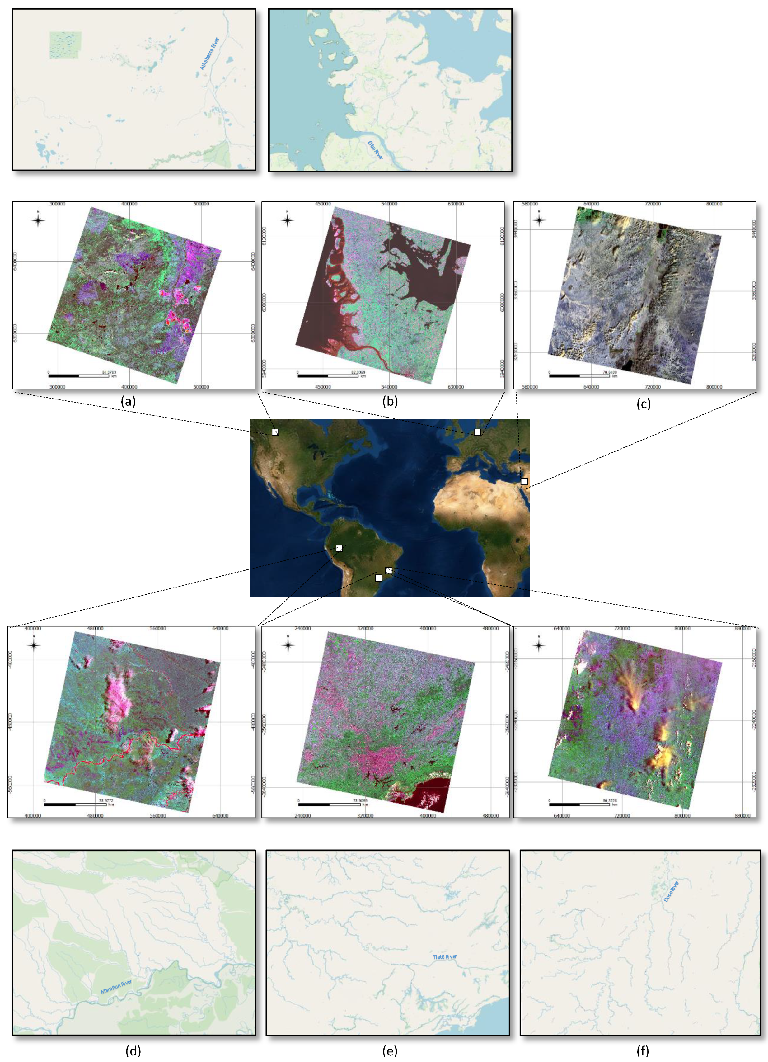
5.2. Study Areas
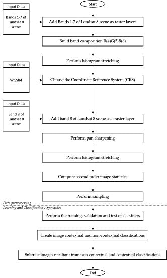
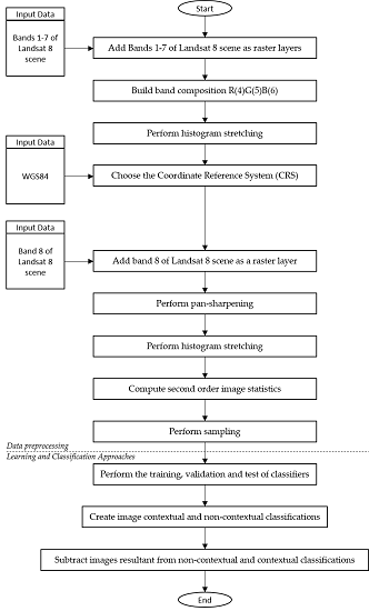
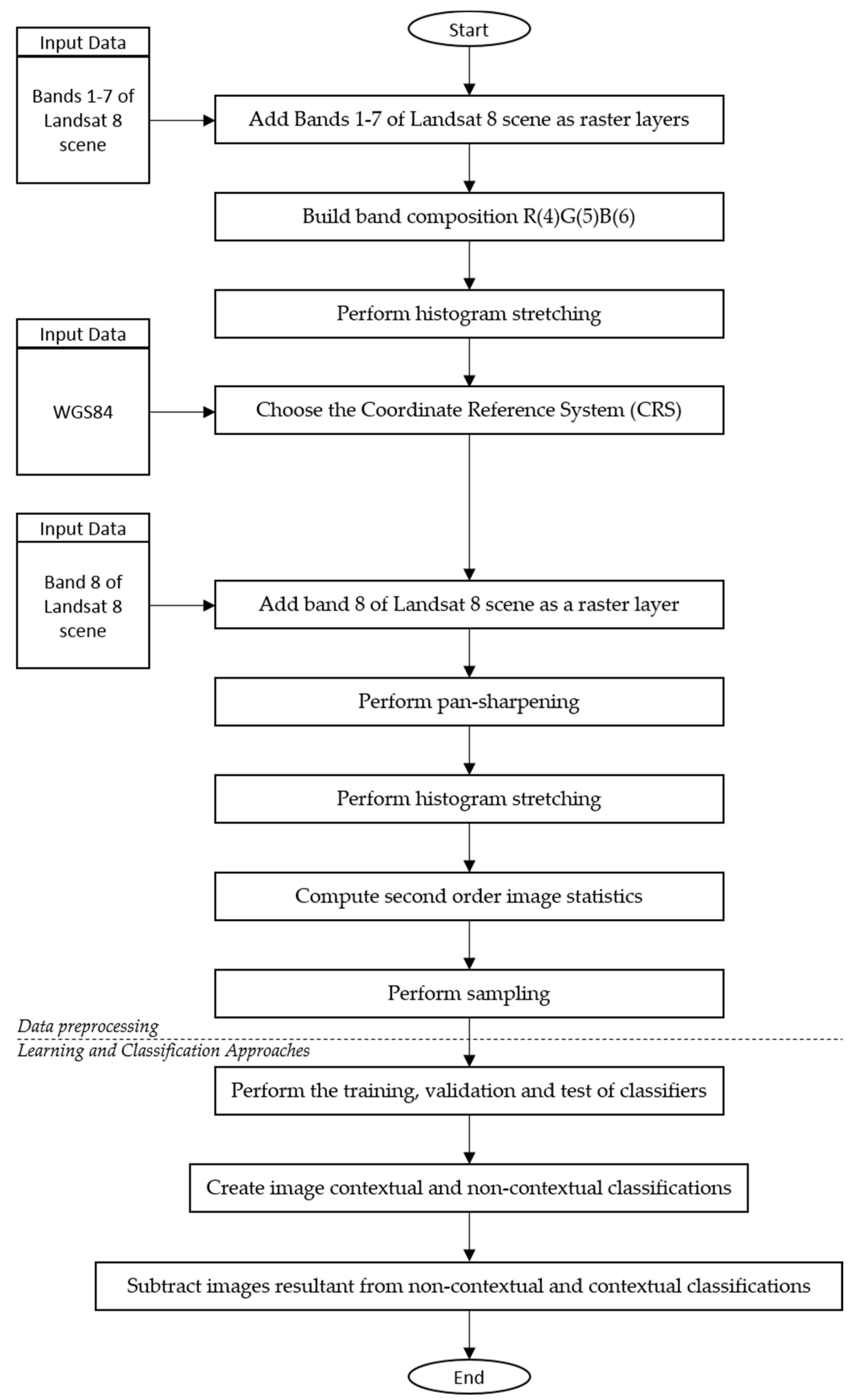
5.3. Method
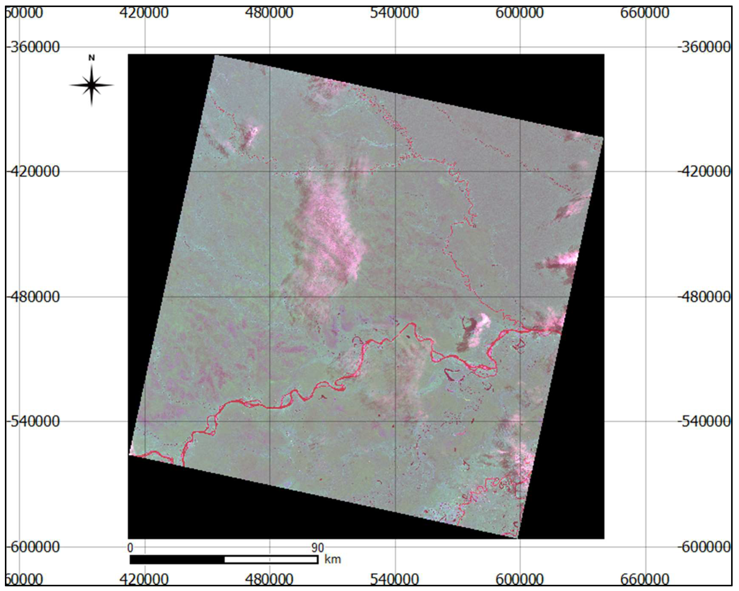
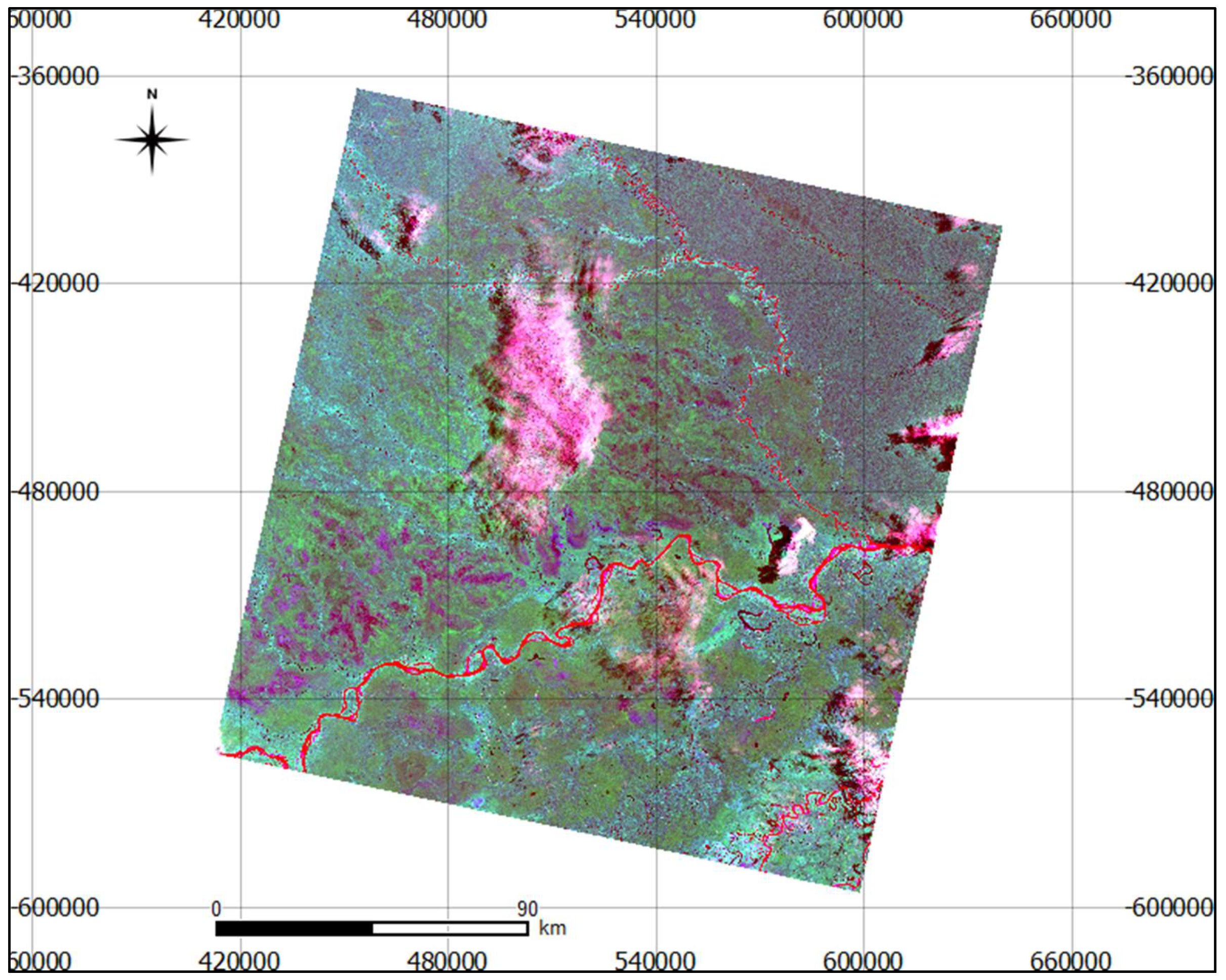
5.3.1. Data Preprocessing
“(...) averaging over all directions φ and all images in the ensemble, it is found that on log-log scale power as function of frequency f lies approximately on a straight line (...) This means that spectral power as function of spatial frequency behaves according to a power law function. Moreover, fitting a line through the data points yields a slope α of approximately negative two for natural images:Here, α ≈ −2 is the spectral slope, η is its deviation from −2, and constant A describes the overall image contrast.”
5.3.2. Learning and Classification Approaches
6. Results
6.1. Experimental Results
6.2. Interpretation of the Results
7. Discussion
8. Conclusions
Author Contributions
Funding
Acknowledgments
Conflicts of Interest
Appendix A
Appendix A.1. Sampling

Appendix A.2. Rendering
Appendix A.3. UTM Projection
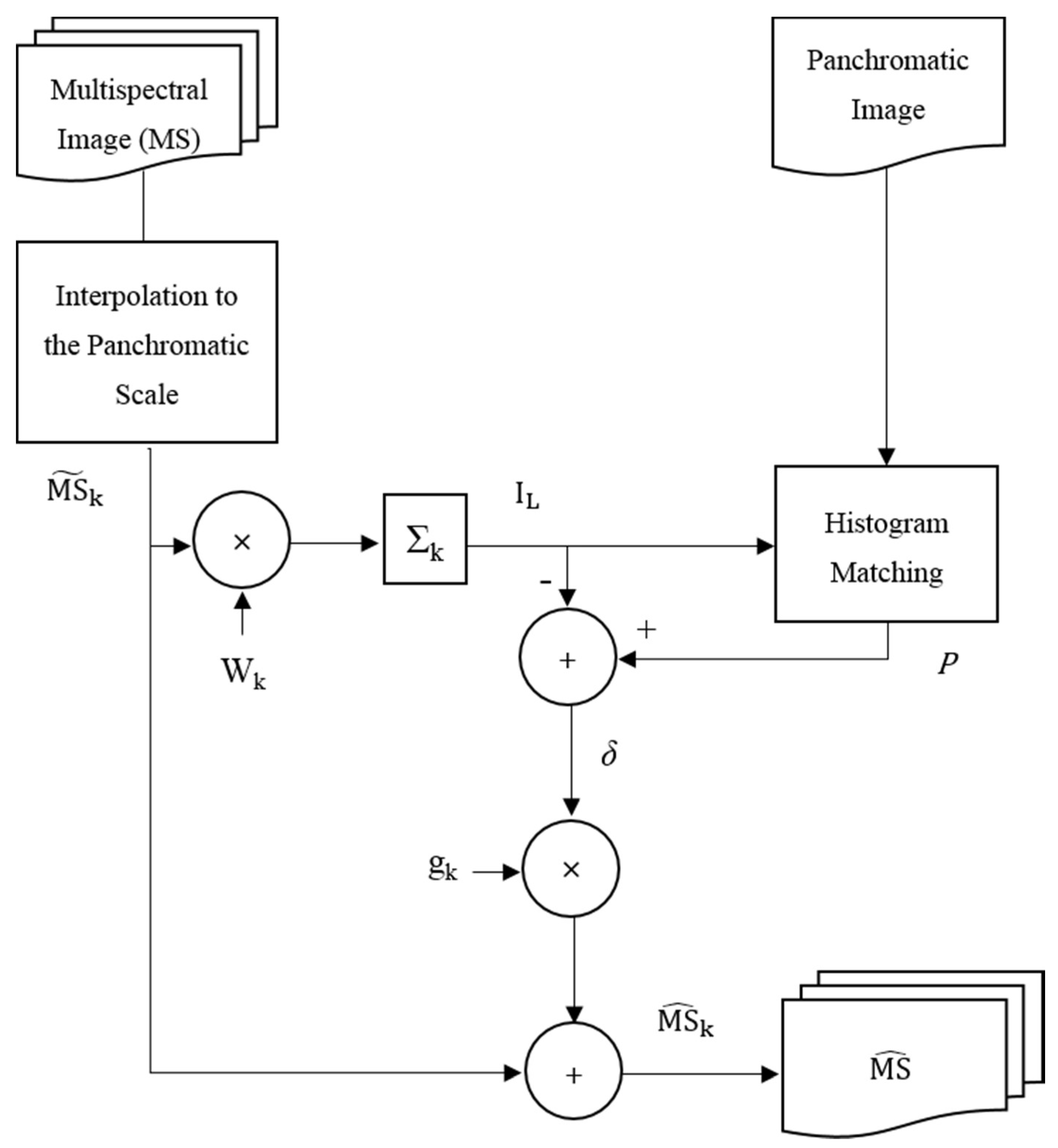
Appendix A.4. Pan-Sharpening
Appendix A.5. Learning and Classification Approaches

References
- Li, W.; Du, Q. A survey on representation-based classification and detection in hyperspectral remote sensing imagery. Pattern Recognit. Lett. 2016, 83, 115–123. [Google Scholar] [CrossRef]
- Yang, K.; Li, M.; Liu, Y.; Cheng, L.; Huang, Q.; Chen, Y. River detection in remotely sensed imagery using Gabor Filtering and path opening. Remote Sens. 2015, 7, 8779–8802. [Google Scholar] [CrossRef] [Green Version]
- Chen, C.H. Handbook of Pattern Recognition and Computer Vision, 5th ed.; World Scientific: Singapore, 2015. [Google Scholar]
- Xie, X.; Li, B.; Chai, X. Kernel-based Nonparametric Fisher Classifier for Hyperspectral Remote Sensing Imagery. J. Inf. Hiding Multimed. Signal Process. 2015, 6, 591–599. [Google Scholar]
- Li, M.; Zang, S.; Zhang, B.; Li, S.; Wu, C. A review of remote sensing image classification techniques: The role of spatio-contextual information. Eur. J. Remote Sens. 2014, 47, 389–411. [Google Scholar] [CrossRef]
- Perveen, N.; Kumar, D.; Bhardwaj, I. An overview on template matching methodologies and its applications. Int. J. Res. Comput. Commun. Technol. 2013, 2, 988–995. [Google Scholar]
- Jiang, D.; Zhuang, D.; Huang, Y.; Fu, J. Survey of multispectral image fusion techniques in remote sensing applications. In Image Fusion and its Applications; Chinese Academy of Sciences: Beijing, China, 2011; pp. 1–23. [Google Scholar]
- Mountrakis, G.; Im, J.; Ogole, C. Support vector machines in remote sensing: A review. ISPRS J. Photogramm. Remote Sens. 2011, 66, 247–259. [Google Scholar] [CrossRef]
- Shen, L.; Li, C. Water Body Extraction from Landsat ETM+ Imagery Using Adaboost Algorithm. In Proceedings of the IEEE 2010 18th International Conference on Geoinformatics, Beijing, China, 18–20 June 2010. [Google Scholar] [CrossRef]
- Dey, V.; Zhang, Y.; Zhong, M. A Review on Image Segmentation Techniques with Remote Sensing Perspective. In Proceedings of the ISPRS TC VII Symposium—100 Years ISPRS, Vienna, Austria, 5–7 July 2010; Wagner, W., Székely, B., Eds.; IAPRS: Paris, France, 2010; Volume XXXVIII. Part 7A. [Google Scholar]
- Schowengerdt, R.A. Remote Sensing: Models and Methods for Image Processing, 3rd ed.; Elsevier: London, UK, 2006. [Google Scholar]
- Richards, J.A.; Jia, X. Remote Sensing Digital Image Analysis, 1st ed.; Springer: Berlin, Germany, 1999. [Google Scholar]
- Kittler, J.; Christmas, W.; de Campos, T.; Windridge, D.; Yan, F.; Illingworth, J.; Osman, M. Domain anomaly detection in machine perception: A system architecture and taxonomy. IEEE Trans. Pattern Anal. Mach. Intell. 2014, 36, 845–859. [Google Scholar] [CrossRef] [Green Version]
- Chandola, V.; Banerjee, A.; Kumar, V. Anomaly detection: A survey. ACM Comput. Surv. (CSUR) 2009, 41, 1–72. [Google Scholar] [CrossRef]
- Weinshall, D.; Zweig, A.; Hermansky, H.; Kombrink, S.; Ohl, F.W.; Anemuller, J.; Bach, J.-H.; Gool, L.V.; Nater, F.; Pajdla, T.; et al. Beyond novelty detection: Incongruent events, when general and specific classifiers disagree. IEEE Trans. Pattern Anal. Mach. Intell. 2012, 34, 1886–1901. [Google Scholar] [CrossRef] [Green Version]
- Ponti, M.; Kittler, J.; Riva, M.; de Campos, T.; Zor, C. A decision cognizant Kullback–Leibler divergence. Pattern Recognit. 2017, 61, 470–478. [Google Scholar] [CrossRef] [Green Version]
- Kittler, J.; Zor, C. Delta divergence: A novel decision cognizant measure of classifier incongruence. IEEE Trans. Cybern. 2018, 99, 1–13. [Google Scholar] [CrossRef] [PubMed]
- Kittler, J.; Zor, C. A Measure of Surprise for Incongruence Detection. In Proceedings of the 2nd International Conference on Intelligent Signal Processing (ISP), London, UK, 1–2 December 2015; IET: London, UK, 2015; pp. 1–6. [Google Scholar] [CrossRef]
- Chandola, V.; Banerjee, A.; Kumar, V. Outlier detection: A survey. ACM Comput. Surv. (CSUR) 2007, 14, 1–83. [Google Scholar]
- Gupta, M.; Gao, J.; Aggarwal, C.C.; Han, J. Outlier detection for temporal data: A survey. IEEE Trans. Knowl. Data Eng. 2013, 26, 2250–2267. [Google Scholar] [CrossRef]
- Zimek, A.; Schubert, E.; Kriegel, H.P. A survey on unsupervised outlier detection in high-dimensional numerical data. Stat. Anal. Data Min. ASA Data Sci. J. 2012, 5, 363–387. [Google Scholar] [CrossRef]
- Gogoi, P.; Bhattacharyya, D.K.; Borah, B.; Kalita, J.K. A survey of outlier detection methods in network anomaly identification. Comput. J. 2011, 54, 570–588. [Google Scholar] [CrossRef] [Green Version]
- Niu, Z.; Shi, S.; Sun, J.; He, X. A Survey of Outlier Detection Methodologies and Their Applications. In Proceedings of the International Conference on Artificial Intelligence and Computational Intelligence, Taiyuan, China, 24–25 October 2011; Springer: Berlin/Heidelberg, Germany, 2011; pp. 380–387. [Google Scholar]
- Hodge, V.; Austin, J. A survey of outlier detection methodologies. Artif. Intell. Rev. 2004, 22, 85–126. [Google Scholar] [CrossRef] [Green Version]
- Liu, Q.; Klucik, R.; Chen, C.; Grant, G.; Gallaher, D.; Lv, Q.; Shang, L. Unsupervised detection of contextual anomaly in remotely sensed data. Remote Sens. Environ. 2017, 202, 75–87. [Google Scholar] [CrossRef]
- Data Management and Information Distribution (DMID)—Landsat Data Dictionary. Available online: https://lta.cr.usgs.gov/DD/landsat_dictionary.html#image_quality_landsat_8 (accessed on 29 August 2019).
- Blanzieri, E.; Melgani, F. Nearest Neighbor Classification of remote sensing images with the maximal margin principle. IEEE Trans. Geosci. Remote Sens. 2008, 46, 1804–1811. [Google Scholar] [CrossRef]
- Ma, L.; Crawford, M.M.; Tian, J. Local manifold learning-based k-Nearest-Neighbor for hyperspectral image classification. IEEE Trans. Geosci. Remote Sens. 2010, 48, 4099–4109. [Google Scholar] [CrossRef]
- Swain, P.H.; Hauska, H. The decision tree classifier: Design and potential. IEEE Trans. Geosci. Electron. 1977, 15, 142–147. [Google Scholar] [CrossRef]
- Yi-Bin, L.; Ying-Ying, W.; Xue-Wen, R. Improvement of ID3 Algorithm Based on Simplified Information Entropy and Coordination Degree. In Proceedings of the Chinese Automation Congress (CAC), Jinan, China, 20–22 October 2017; IEEE: Toulouse, France, 2017; pp. 1526–1530. [Google Scholar] [CrossRef]
- Fernandes, G.W.; Goulart, F.F.; Ranieri, B.D.; Coelho, M.S.; Dales, K.; Boesche, N.; Bustamante, M.; Carvalho, F.A.; Carvalho, D.C.; Dirzo, R.; et al. Deep into the mud: Ecological and socio-economic impacts of the dam breach in Mariana, Brazil. Braz. J. Nat. Conserv. 2016, 14, 35–45. [Google Scholar] [CrossRef]
- Mielke, C.; Boesche, N.K.; Rogass, C.; Kaufmann, H.; Gauert, C.; de Wit, M. Spaceborne mine waste mineralogy monitoring in South Africa, applications for modern push-broom missions: Hyperion/OLI and EnMAP/Sentinel-2. Remote Sens. 2014, 6, 6790–6816. [Google Scholar] [CrossRef] [Green Version]
- Rosell-Melé, A.; Moraleda-Cibrián, N.; Cartró-Sabaté, M.; Colomer-Ventura, F.; Mayor, P.; Orta-Martínez, M. Oil pollution in soils and sediments from the Northern Peruvian Amazon. Sci. Total Environ. 2018, 610, 1010–1019. [Google Scholar] [CrossRef] [PubMed]
- Asht, S.; Dass, R. Pattern recognition techniques: A review. Int. J. Comput. Sci. Telecommun. 2012, 3, 25–29. [Google Scholar]
- Bishop, C.M. Pattern Recognition and Machine Learning, 1st ed.; Springer: Berlin/Heidelberg, Germany, 2006. [Google Scholar]
- Jahne, B. Computer Vision and Applications: A guide for Students and Practitioners, 1st ed.; Elsevier: London, UK, 2000. [Google Scholar]
- Ye, Q.-Z.; Wu, P.; Zhang, M.-L. Research on Automatic Highway Extraction Technology Based on Spectral Information of Remote Sensing Images. J. Inf. Hiding Multimed. Signal Proc. 2017, 8, 368–380. [Google Scholar]
- Chaker, R.; Al Aghbari, Z.; Junejo, I.N. Social network model for crowd anomaly detection and localization. Pattern Recognit. 2017, 61, 266–281. [Google Scholar] [CrossRef]
- Ahmed, M.; Mahmood, A.N.; Islam, M.R. A survey of anomaly detection techniques in financial domain. Future Gener. Comput. Syst. 2016, 55, 278–288. [Google Scholar] [CrossRef]
- Ahmed, M.; Mahmood, A.N.; Hu, J. A survey of network anomaly detection techniques. J. Netw. Comput. Appl. 2016, 60, 19–31. [Google Scholar] [CrossRef]
- Agrawal, S.; Agrawal, J. Survey on anomaly detection using data mining techniques. Procedia Comput. Sci. 2015, 60, 708–713. [Google Scholar] [CrossRef] [Green Version]
- Akoglu, L.; Tong, H.; Koutra, D. Graph based anomaly detection and description: A survey. Data Min. Knowl. Discov. 2015, 29, 626–688. [Google Scholar] [CrossRef] [Green Version]
- Pawar, A.D.; Kalavadekar, P.N.; Tambe, S.N. A survey on outlier detection techniques for credit card fraud detection. IOSR J. Comput. Eng. 2014, 16, 44–48. [Google Scholar] [CrossRef]
- Zhang, J. Advancements of outlier detection: A survey. ICST Trans. Scalable Inf. Syst. 2013, 13, 1–26. [Google Scholar] [CrossRef] [Green Version]
- Lin, A.Y.M.; Novo, A.; Har-Noy, S.; Ricklin, N.D.; Stamatiou, K. Combining GeoEye-1 satellite remote sensing, UAV aerial imaging, and geophysical surveys in anomaly detection applied to archaeology. IEEE J. Sel. Top. Appl. Earth Obs. Remote Sens. 2011, 4, 870–876. [Google Scholar] [CrossRef]
- Xie, M.; Han, S.; Tian, B.; Parvin, S. Anomaly detection in wireless sensor networks: A survey. J. Netw. Comput. Appl. 2011, 34, 1302–1325. [Google Scholar] [CrossRef]
- Chandola, V.; Banerjee, A.; Kumar, V. Anomaly detection for discrete sequences: A survey. IEEE Trans. Knowl. Data Eng. 2010, 24, 823–839. [Google Scholar] [CrossRef]
- Zhang, W.; Yang, Q.; Geng, Y. A Survey of Anomaly Detection Methods in Networks. In Proceedings of the International Symposium on Computer Network and Multimedia Technology, Wuhan, China, 18–20 January 2009; IEEE: Toulouse, France, 2009; pp. 1–3. [Google Scholar] [CrossRef]
- Congalton, R.G.; Green, K. Assessing the Accuracy of Remotely Sensed Data: Principles and Practices, 2nd ed.; CRC Press: Boca Raton, FL, USA, 2008. [Google Scholar]
- Transon, J.; d’Andrimont, R.; Maugnard, A.; Defourny, P. Survey of hyperspectral earth observation applications from space in the sentinel-2 context. Remote Sens. 2018, 10, 157. [Google Scholar] [CrossRef] [Green Version]
- Frontera-Pons, J.; Veganzones, M.A.; Pascal, F.; Ovarlez, J.P. Hyperspectral anomaly detectors using robust estimators. IEEE J. Sel. Top. Appl. Earth Obs. Remote Sens. 2015, 9, 720–731. [Google Scholar] [CrossRef] [Green Version]
- Matteoli, S.; Diani, M.; Theiler, J. An overview of background modeling for detection of targets and anomalies in hyperspectral remotely sensed imagery. IEEE J. Sel. Top. Appl. Earth Obs. Remote Sens. 2014, 7, 2317–2336. [Google Scholar] [CrossRef]
- Matteoli, S.; Veracini, T.; Diani, M.; Corsini, G. Models and methods for automated background density estimation in hyperspectral anomaly detection. IEEE J. Sel. Top. Appl. Earth Obs. Remote Sens. 2012, 51, 2837–2852. [Google Scholar] [CrossRef]
- Matteoli, S.; Diani, M.; Corsini, G. A tutorial overview of anomaly detection in hyperspectral images. IEEE Aerosp. Electron. Syst. Mag. 2010, 25, 5–28. [Google Scholar] [CrossRef]
- Nazeer, M.; Nichol, J.E. Combining Landsat TM/ETM+ and HJ-1 A/B CCD sensors for monitoring coastal water quality in Hong Kong. IEEE Geosci. Remote Sens. Lett. 2015, 12, 1898–1902. [Google Scholar] [CrossRef]
- Ha, N.T.T.; Koike, K.; Nhuan, M.T.; Canh, B.D.; Thao, N.T.P.; Parsons, M. Landsat 8/OLI two bands ratio algorithm for Chlorophyll-A concentration mapping in hypertrophic waters: An application to West Lake in Hanoi (Vietnam). IEEE J. Sel. Top. Appl. Earth Obs. Remote Sens. 2017, 10, 4919–4929. [Google Scholar] [CrossRef]
- Chen, J.; Zhu, W.-N.; Tian, Y.Q.; Yu, Q. Estimation of colored dissolved organic matter from Landsat-8 imagery for complex inland water: Case study of Lake Huron. IEEE Trans. Geosci. Remote Sens. 2017, 55, 2201–2212. [Google Scholar] [CrossRef]
- Kotchi, S.O.; Brazeau, S.; Turgeon, P.; Pelcat, Y.; Légaré, J.; Lavigne, M.-P.; Essono, F.N.; Fournier, R.A.; Michel, P. Evaluation of Earth observation systems for estimating environmental determinants of microbial contamination in recreational waters. IEEE J. Sel. Top. Appl. Earth Obs. Remote Sens. 2015, 8, 3730–3741. [Google Scholar] [CrossRef]
- Chang, N.-B.; Vannah, B.; Yang, Y.J. Comparative sensor fusion between hyperspectral and multispectral satellite sensors for monitoring microcystin distribution in Lake Erie. IEEE J. Sel. Top. Appl. Earth Obs. Remote Sens. 2014, 7, 2426–2442. [Google Scholar] [CrossRef]
- Li, Z.; Liu, H.; Luo, C.; Li, P.; Li, H.; Xiong, Z. Industrial wastewater discharge retrieval based on stable nighttime light imagery in China from 1992 to 2010. Remote Sens. 2014, 6, 7566–7579. [Google Scholar] [CrossRef] [Green Version]
- Mustard, J.F.; Sunshine, J.M. Spectral analysis for earth science: Investigations using remote sensing data. Remote Sens. Earth Sci. Man. Remote Sens. 1999, 3, 251–307. [Google Scholar]
- Verstraete, M.M.; Pinty, B. Designing optimal spectral indexes for remote sensing applications. IEEE Trans. Geosci. Remote Sens. 1996, 34, 1254–1265. [Google Scholar] [CrossRef]
- Brezonik, P.L.; Olmanson, L.G.; Finlay, J.C.; Bauer, M.E. Factors affecting the measurement of CDOM by remote sensing of optically complex inland waters. Remote Sens. Environ. 2015, 157, 199–215. [Google Scholar] [CrossRef]
- Xie, X.; Li, B. A Unified Framework of Multiple Kernels Learning for Hyperspectral Remote Sensing Big Data. J. Inf. Hiding Multimed. Signal Process 2016, 7, 296–303. [Google Scholar]
- Li, Y.; Li, J.; Pan, J.-S. Hyperspectral Image Recognition Using SVM Combined Deep Learning. J. Internet Technol. 2019, 20, 851–859. [Google Scholar]
- Sublime, J.; Kalinicheva, E. Automatic post-disaster damage mapping using deep-learning techniques for change detection: Case study of the Tohoku tsunami. Remote Sens. 2019, 11, 1123. [Google Scholar] [CrossRef] [Green Version]
- Tan, C.; Sun, F.; Kong, T.; Zhang, W.; Yang, C.; Liu, C. A Survey on Deep Transfer Learning. In Proceedings of the International Conference on Artificial Neural Network, Rhodes, Greece, 4–7 October 2018; Springer: Cham, Switzerland, 2018; pp. 270–279. [Google Scholar]
- Lu, J.; Behbood, V.; Hao, P.; Zuo, H.; Xue, S.; Zhang, G. Transfer learning using computational intelligence: A survey. Knowl. Based Syst. 2015, 80, 14–23. [Google Scholar] [CrossRef]
- Shao, L.; Zhu, F.; Li, X. Transfer learning for visual categorization: A survey. IEEE Trans. Neural Netw. Learn. Syst. 2014, 26, 1019–1034. [Google Scholar] [CrossRef] [PubMed]
- Cook, D.; Feuz, K.D.; Krishnan, N.C. Transfer learning for activity recognition: A survey. Knowl. Inf. Syst. 2013, 36, 537–556. [Google Scholar] [CrossRef] [PubMed] [Green Version]
- Sun, S. A survey of multi-view machine learning. Neural Comput. Appl. 2013, 23, 2031–2038. [Google Scholar] [CrossRef]
- Xu, Q.; Yang, Q. A survey of transfer and multitask learning in bioinformatics. J. Comput. Sci. Eng. 2011, 5, 257–268. [Google Scholar] [CrossRef] [Green Version]
- Pan, S.J.; Yang, Q. A survey on transfer learning. IEEE Trans. Knowl. Data Eng. 2010, 22, 1345–1359. [Google Scholar] [CrossRef]
- Taylor, M.E.; Stone, P. Transfer learning for reinforcement learning domains: A survey. J. Mach. Learn. Res. 2009, 10, 1633–1685. [Google Scholar]
- Committee on Developments in the Science of Learning, Committee on Learning Research and Educational Practice & National Research Council. In How People Learn: Brain, Mind, Experience, and School, Expanded ed.; National Academy Press: Washington, DC, USA, 2000.
- Shoujing, Y.; Qiao, W.; Chuanqing, W.; Xiaoling, C.; Wandong, M.; Huiqin, M. A robust anomaly based change detection method for time-series remote sensing images. In IOP Conference Series: Earth and Environmental Science; IOP Publishing Ltd.: Bristol, UK, 2014; Volume 17, p. 012059. [Google Scholar]
- Zhou, Z.-G.; Tang, P.; Zhou, M. Detecting Anomaly Regions in Satellite Image Time Series Based on Seasonal Autocorrelation Analysis. In Proceedings of the ISPRS Annals of the Photogrammetry, Remote Sensing Spatial Information Science (XXIII ISPRS Congress), Prague, Czech Republic, 12–19 July 2016; pp. 303–310. [Google Scholar]
- Chandola, V.; Vatsavai, R.R. A Gaussian Process Based Online Change Detection Algorithm for Monitoring Periodic Time Series. In Proceedings of the 2011 SIAM International Conference on Data Mining, Society for Industrial and Applied Mathematics, Mesa, AZ, USA, 28–30 April 2011; pp. 95–106. [Google Scholar] [CrossRef] [Green Version]
- Tan, P.-N.; Steinbach, M.; Karpatne, A.; Kumar, V. Introduction to Data Mining, 2nd ed.; Pearson Education: Noida, India, 2018. [Google Scholar]
- Bhaduri, K.; Das, K.; Votava, P. Distributed Anomaly Detection Using Satellite Data from Multiple Modalities. In Proceedings of the 2010 Conference on Intelligent Data Understanding, CIDU 2010, Mountain View, CA, USA, 5–6 October 2010. [Google Scholar]
- Bormann, K.J.; McCabe, M.F.; Evans, J.P. Satellite based observations for seasonal snow cover detection and characterization in Australia. Remote Sens. Environ. 2012, 123, 57–71. [Google Scholar] [CrossRef]
- Chen, C.; Yang, B.; Song, S.; Peng, X.; Huang, R. Automatic clearance anomaly detection for transmission line corridors utilizing UAV-Borne LIDAR Data. Remote Sens. 2018, 10, 613. [Google Scholar] [CrossRef] [Green Version]
- USGS—The United States Geological Survey, “Earth Explorer”. Available online: https://earthexplorer.usgs.gov/ (accessed on 25 April 2018).
- QGIS Development Team. Available online: https://www.qgis.org/ (accessed on 25 April 2018).
- Gordon, G.; Stavi, I.; Shavit, U.; Rosenzweig, R. Oil spill effects on soil hydrophobicity and related properties in a hyper-arid region. Geoderma 2018, 312, 114–120. [Google Scholar] [CrossRef]
- Pisano, A.; Bignami, F.; Santoleri, R. Oil spill detection in glint-contaminated near-infrared MODIS imagery. Remote Sens. 2015, 7, 1112–1134. [Google Scholar] [CrossRef] [Green Version]
- Reátegui-Zirena, E.G.; Stewart, P.M.; Whatley, A.; Chu-Koo, F.; Sotero-Solis, V.E.; Merino-Zegarra, C.; Vela-Paima, E. Polycyclic aromatic hydrocarbon concentrations, mutagenicity, and Microtox® acute toxicity testing of Peruvian crude oil and oil-contaminated water and sediment. Environ. Monit. Assess. 2014, 186, 2171–2184. [Google Scholar] [CrossRef] [PubMed]
- Gonzales, R.C.; Woods, R.E. Digital Image Processing, 2nd ed.; Prentice Hall: Upper Saddle River, NJ, USA, 2002. [Google Scholar]
- QGIS Project. QGIS User Guide Release 2.14. 2017. Available online: https://docs.qgis.org/2.14/pdf/en/QGIS-2.14-UserGuide-en.pdf (accessed on 25 April 2018).
- OTB Development Team. The Orfeo ToolBox Cookbook, a Guide for Non-Developers Updated for OTB-3.10. 2011. Available online: https://www.orfeo-toolbox.org/packages/archives/Doc/CookBook-310.pdf (accessed on 25 April 2018).
- Vivone, G.; Alparone, L.; Chanussot, J.; Mura, M.D.; Garzelli, A.; Licciardi, G.A.; Restaino, R.; Wald, L. A critical comparison among pansharpening algorithms. IEEE Trans. Geosci. Remote Sens. 2015, 53, 2565–2586. [Google Scholar] [CrossRef]
- OTB Development Team. The On-Line Orfeo ToolBox Cookbook, a Guide for Non-Developers Updated for OTB-3.10. 2011. Available online: https://www.orfeo-toolbox.org/packages/doc/tests-rfc-52/cookbook-3b41671/Applications/app_Superimpose.html; Available online: https://www.qgis.org/ (accessed on 25 April 2018).
- Reinhard, E.; Shirley, P.; Ashikhmin, M.; Troscianko, T. Second Order Image Statistics in Computer Graphics. In Proceedings of the 1st Symposium on Applied Perception in Graphics and Visualization (APGV’04), Los Angeles, CA, USA, 7–8 August 2004; pp. 99–106. [Google Scholar]
- OTB Development Team. The On-Line Orfeo ToolBox Cookbook, a Guide for Non-Developers Updated for OTB-3.10. 2011. Available online: https://www.orfeo-toolbox.org/packages/doc/tests-rfc-52/cookbook-3b41671/Applications/app_TrainImagesClassifier.html (accessed on 25 April 2018).
- Congalton, R.G.; Mead, R.A. A review of three discrete multivariate analysis techniques used in assessing the accuracy of remotely sensed data from error matrices. IEEE Trans. Geosci. Remote Sens. 1986, GE-24, 169–174. [Google Scholar] [CrossRef]
- Marzano, F.S.; Scaranari, D.; Montopoli, M.; Vulpiani, G. Supervised classification and estimation of hydrometeors from C-Band dual-polarized radars: A Bayesian approach. IEEE Trans. Geosci. Remote Sens. 2008, 46, 85–98. [Google Scholar] [CrossRef]
- Indu, J.; Kumar, D.N. Evaluation of precipitation retrievals from orbital data products of TRMM over a subtropical basin in India. IEEE Trans. Geosci. Remote Sens. 2015, 53, 6429–6442. [Google Scholar] [CrossRef]
- Che, X.; Feng, M.; Sexton, J.; Channan, S.; Sun, Q.; Ying, Q.; Liu, J.; Wang, Y. Landsat-based estimation of seasonal water cover and change in arid and semi-arid Central Asia (2000–2015). Remote Sens. 2019, 11, 1323. [Google Scholar] [CrossRef] [Green Version]
- Chen, Y.; Fan, R.; Yang, X.; Wang, J.; Latif, A. Extraction of urban water bodies from high-resolution remote-sensing imagery using deep learning. Water 2018, 10, 585. [Google Scholar] [CrossRef] [Green Version]
- Natesan, S.; Armenakis, C.; Benari, G.; Lee, R. Use of UAV-borne spectrometer for land cover classification. Drones 2018, 2, 16. [Google Scholar] [CrossRef] [Green Version]
- Bernardo, N.; do Carmo, A.; Park, E.; Alcântara, E. Retrieval of suspended particulate matter in inland waters with widely differing optical properties using a semi-analytical scheme. Remote Sens. 2019, 11, 2283. [Google Scholar] [CrossRef] [Green Version]
- Snyder, J.P. Map projections: A working manual. In US Geological Survey Professional Paper 1395; United States Government Printing Office: Washington, DC, USA, 1987. [Google Scholar]


| Environment and Country | UTM Zone and Center: Latitude/Longitude | Disaster | Landsat 8 Image (Scene) | Date of the: Image Acquisition/Environmental Disaster | Number of Samples |
|---|---|---|---|---|---|
| Doce River Brazil | 23 20°13′48.07″S 42°43′47.24″W | Dam Breach | LC08_L1TP_217074_20151112_20170402_01_T1 | 12 November 2015 5 November 2015 | 250 |
| Athabasca River Canada | 12 57°18′35.86″N 112°33′13.21″W | ______ | LC08_L1TP_043020_20170826_20170913_01_T1 | 26 August 2017 No Disaster | 100 |
| Elbe River Germany | 32 54°30′31.36″N 9°29′07.80″E | ______ | LC08_L1TP_196022_20180509_20180517_01_T1 | 9 May 2018 No Disaster | 100 |
| Marañon River Peru | 18 4°20′20.54″S 74°45′45.97″W | Pipeline Disruption | LC08_L1TP_007063_20160827_20170321_01_T1 | 27 August 2016 22 August 2016 | 100 |
| Tietê River Brazil | 23 23°06′46.33″S 46°30′16.96″W | Permanent Sewage Disposal | LC08_L1TP_219076_20170827_20170914_01_T1 | 27 August 2017 Permanently | 100 |
| Arava Valley Israel | 36 30°18′22.86″N 35°02′25.51″E | Pipeline Disruption | LC08_L1TP_174039_20141214_20170416_01_T1 | 14 December 2014 4 December 2014 | 100 |
| Environment and Country | Basin Size | Length of the River | Predominant Features in the Environment | Human Activity in the Region | Potential Threat to the Environment | Potential Contaminators or Contaminators |
|---|---|---|---|---|---|---|
| Doce River Brazil | 83,400 km2 (32,201 sq mi) | 853 km (530 mi) | Mountains and Valleys | Mining | Ore Tailings Reservoirs | Brown Mud |
| Athabasca River Canada | 95,300 km2 (36,800 sq mi) | 1231 km (765 mi) | Lakes | Mining | Ore Tailings Reservoirs | Brown and Red Mud |
| Elbe River Germany | 148,268 km2 (57,247 sq mi) | 1094 km (680 mi) | Close to the Coastline | Mining | Ore Tailings Reservoirs | Red Mud |
| Marañon River Peru | 358,000 km2 (138,000 sq mi) | 1737 km (1079 mi) | Forest | Transport of Crude Oil | Oil Pipeline | Crude Oil |
| Tietê River Brazil | 150,000 km2 (58,000 sq mi) | 1150 km (710 mi) | Densely Populated Region | Sewage Disposal | Sewer | Sewage |
| Arava Valley Israel | ______ | ______ | Arid Valley | Transport of Crude Oil | Oil Pipeline | Crude Oil |
| Environment Country | Landsat 8 Scene | Scene Resolution (Height and Width in Pixels) | Image Tile Resolution (Height and Width in Pixels) | Total Number of Tiles |
|---|---|---|---|---|
| Doce River Brazil | LC08_L1TP_217074_20151112_20170402_01_T1 | 15705 × 15440 | 151 × 193 | 8400 |
| Athabasca River Canada | LC08_L1TP_043020_20170826_20170913_01_T1 | 16499 × 16277 | 146 × 155 | 11836 |
| Elbe River Germany | LC08_L1TP_196022_20180509_20180517_01_T1 | 16099 × 15882 | 145 × 143 | 12544 |
| Marañon River Peru | LC08_L1TP_007063_20160827_20170321_01_T1 | 15498 × 15185 | 126 × 146 | 12792 |
| Tietê River Brazil | LC08_L1TP_219076_20170827_20170914_01_T1 | 15484 × 15250 | 139 × 162 | 14641 |
| Arava Valley Israel | LC08_L1TP_174039_20141214_20170416_01_T1 | 15432 × 15067 | 129 × 127 | 10528 |
| Incongruent Event | Congruent Event | |
|---|---|---|
| Detection Incongruent | TP = 68 | FP = 20 |
| Detection Congruent | FN = 0 | TN = 8312 |
| Incongruent Event | Congruent Event | |
|---|---|---|
| Detection Incongruent | TP = 87 | FP = 38 |
| Detection Congruent | FN = 0 | TN = 11,959 |
| Incongruent Event | Congruent Event | |
|---|---|---|
| Detection Incongruent | TP = 0 | FP = 18 |
| Detection Congruent | FN = 0 | TN = 12,526 |
| Incongruent Event | Congruent Event | |
|---|---|---|
| Detection Incongruent | TP = 39 | FP = 13 |
| Detection Congruent | FN = 0 | TN = 12,863 |
| Incongruent Event | Congruent Event | |
|---|---|---|
| Detection Incongruent | TP = 0 | FP = 25 |
| Detection Congruent | FN = 0 | TN = 10,503 |
| Incongruent Event | Congruent Event | |
|---|---|---|
| Detection Incongruent | TP = 0 | FP = 0 |
| Detection Congruent | FN = 0 | TN = 14,641 |
| Landsat 8 Scene | Environment | Accuracy | Precision | Recall | F-Measure |
|---|---|---|---|---|---|
| LC08_L1TP_217074_20151112_20170402_01_T1 | Doce River Basin | ~99.76% | ~77.27% | 100% | 87.18% |
| LC08_L1TP_043020_20170826_20170913_01_T1 | Athabasca River Basin | ~99.69% | ~69.6% | 100% | 82.08% |
| LC08_L1TP_007063_20160827_20170321_01_T1 | Marañon River Basin | ~99.90% | 75% | 100% | 85.71% |
| Study | Accuracy | Precision | Recall | F-Measure |
|---|---|---|---|---|
| Ours | ~99.78% | ~73.96% | 100.00% | 85.04% |
| [98] | 99.59% | ---------- | ---------- | ---------- |
| [81] | 99.20% | 91.85% | 53.55% | 67.66% |
| [99] | 99.14% | ---------- | ---------- | ---------- |
| [76] | 98.49% | 83.84% | 83.66% | 83.76% |
| [80] | 98.00% | ---------- | ---------- | ---------- |
| [25] | ~91.20% | 98.10% | 95.7% | 96.88% |
| [77] | 88.68% | 90.62% | 79.62% | 84.76% |
| [66] | 84.00% | 63.00% | 81.00% | 70.88% |
| [100] | 81.18% | ---------- | ---------- | ---------- |
| [78] | 78.00% | 82.00% | 75.00% | 78.34% |
| [82] | ---------- | 96.50% | 94.8% | 95.64% |
© 2019 by the authors. Licensee MDPI, Basel, Switzerland. This article is an open access article distributed under the terms and conditions of the Creative Commons Attribution (CC BY) license (http://creativecommons.org/licenses/by/4.0/).
Share and Cite
Dias, M.A.; Silva, E.A.d.; Azevedo, S.C.d.; Casaca, W.; Statella, T.; Negri, R.G. An Incongruence-Based Anomaly Detection Strategy for Analyzing Water Pollution in Images from Remote Sensing. Remote Sens. 2020, 12, 43. https://0-doi-org.brum.beds.ac.uk/10.3390/rs12010043
Dias MA, Silva EAd, Azevedo SCd, Casaca W, Statella T, Negri RG. An Incongruence-Based Anomaly Detection Strategy for Analyzing Water Pollution in Images from Remote Sensing. Remote Sensing. 2020; 12(1):43. https://0-doi-org.brum.beds.ac.uk/10.3390/rs12010043
Chicago/Turabian StyleDias, Maurício Araújo, Erivaldo Antônio da Silva, Samara Calçado de Azevedo, Wallace Casaca, Thiago Statella, and Rogério Galante Negri. 2020. "An Incongruence-Based Anomaly Detection Strategy for Analyzing Water Pollution in Images from Remote Sensing" Remote Sensing 12, no. 1: 43. https://0-doi-org.brum.beds.ac.uk/10.3390/rs12010043