Exploring the Potential of C-Band SAR in Contributing to Burn Severity Mapping in Tropical Savanna


1
Department of Remote Sensing, University of Würzburg, 97074 Würzburg, Germany
2
CSIRO Land and Water, PMB 44, Winnellie NT 0822, Australia
*
Author to whom correspondence should be addressed.
Remote Sens. 2020, 12(1), 49; https://0-doi-org.brum.beds.ac.uk/10.3390/rs12010049
Submission received: 28 October 2019
/
Revised: 12 December 2019
/
Accepted: 17 December 2019
/
Published: 20 December 2019
(This article belongs to the Special Issue Remote Sensing of Forest Fire: Data, Science and Operational Applications)
Abstract
:The ability to map burn severity and to understand how it varies as a function of time of year and return frequency is an important tool for landscape management and carbon accounting in tropical savannas. Different indices based on optical satellite imagery are typically used for mapping fire scars and for estimating burn severity. However, cloud cover is a major limitation for analyses using optical data over tropical landscapes. To address this pitfall, we explored the suitability of C-band Synthetic Aperture Radar (SAR) data for detecting vegetation response to fire, using experimental fires in northern Australia. Pre- and post-fire results from Sentinel-1 C-band backscatter intensity data were compared to those of optical satellite imagery and were corroborated against structural changes on the ground that we documented through terrestrial laser scanning (TLS). Sentinel-1 C-band backscatter (VH) proved sensitive to the structural changes imparted by fire and was correlated with the Normalised Burn Ratio (NBR) derived from Sentinel-2 optical data. Our results suggest that C-band SAR holds potential to inform the mapping of burn severity in savannas, but further research is required over larger spatial scales and across a broader spectrum of fire regime conditions before automated products can be developed. Combining both Sentinel-1 SAR and Sentinel-2 multi-spectral data will likely yield the best results for mapping burn severity under a range of weather conditions.
1. Introduction
Fire is an integral component of savanna ecosystem functioning and is a key driver of vegetation structure in tree–grass systems around the globe [1]. The tropical savannas of northern Australia are particularly flammable, with many regions burning in two out of every three years [2]. These regions are characterised by distinct dry and wet seasons, and the lack of precipitation from May to October results in very dry and therefore highly flammable fuel-loads [3,4,5]. Thus, fires late in the dry season are of higher intensity than those earlier on in the season and cause greater structural change [6]. Importantly, these late season fires may also result in higher greenhouse gas emissions, and as such, there are policy frameworks in place to encourage a reduction in the frequency of late season burns (the Australian Government’s Emissions Reduction Fund [7]). In order to reduce the risk of large fires with high greenhouse gas emissions, frequent burning early in the dry season is becoming more common [8,9]. The ecological consequences of altering fire regimes is the subject of much debate, and while some suggest that higher biodiversity results from fires with a high temporal and spatial variability [10,11], others warn about a reduction in species diversity and high risks for threatened species [12,13,14]. As such, mapping savanna fires and their severity is important ecologically for understanding ecosystem processes and for quantifying the effects of greenhouse gas mitigation burns as well as socially for informing landscape management and government policies.
Satellite imagery plays an important role in determining the spatial extent and timing of fires in savanna landscapes [15,16]. Course spatial resolution imagery such as Advanced Very High Resolution Radiometer (AVHHR) and Moderate-resolution Imaging Spectroradiometer (MODIS) underpin many operational mapping efforts in north Australian savannas and provide useful insight into detection, timing, and frequency of fires through their high temporal resolution [17]. Landsat-5/-7/-8 and, increasingly, Sentinel-2 are used for higher spatial resolution fire scar mapping in savannas [18,19]. However, mapping the severity is more challenging than mapping just the occurrence of fire, but the integration of Landsat-8 and Sentinel-2 is showing promise [20,21]. One major limitation of all optical remote-sensing approaches is the presence of cloud cover. Masking and atmospheric interference by clouds contributes considerable uncertainty to current fire mapping methods and hinders attempts to understand burn severity. These efforts are complicated even further by the challenge of quantifying severity on the ground.
From a fire ecology and management perspective, the severity of a given fire event is more relevant than frequency and timing alone. Whilst usually correlated to a degree, due to the relationship between time since last fire and available fuel load, large variability in intensity and severity exists in natural landscapes. Quantification of these effects on the ground is challenging, and field-data are often poorly suited for calibration and validation of satellite-based imagery. Moreover, as stated by Jain et al. (2004), the terms “fire severity”, “fire intensity”, and “burn severity” are frequently used interchangeably, causing confusion and miscommunication among land and fire management. “Fire intensity” usually refers to characteristics of the actual fire, including flame length and produced energy [22]. The term severity, on the other hand, typically describes the magnitude of environmental change caused by a fire, e.g., vegetation consumption [23,24]. Since no measurements on the actual fires are compared within this study but rather the degree of post-fire changes on the present vegetation in the form of burn scars as well as the temporal distance at which said changes can still be quantified are studied, we use the term “burn severity” from here on out.
Our goal in this study was to explore the potential for SAR to provide ancillary information for burn severity mapping in tropical savanna landscapes. We hypothesised that SAR backscatter properties would be sensitive to vegetation structural changes caused by fire and that time-series analysis of pre- and post-fire images would contribute to the mapping of burn severity. We contrasted our SAR results against established techniques utilising optical imagery and used terrestrial laser scanning data to interpret our findings.
2. Material and Methods
2.1. Study Area
Our study took place in an established fire experiment in the open savanna woodlands of the Territory Wildlife Park, located approximately 50 km south of Darwin, Australia. The experimental fire treatments (line ignition) were established in 2004, whereby 18 one hectare plots were arranged in three blocks—consisting of 6 fire regime treatments with 3 factor replications [25]. The different treatments include early dry season burning every year (E1), every second year (E2), every third year (E3), and every fifth (E5) year. The remaining two treatments comprise burning late in the dry season every two years (L2) and exclude fire completely (U) (Figure 1).
2.2. Satellite Remote-Sensing Data
In order to assess the utility of C-band SAR for burn severity mapping and to compare it to optical indices, we used imagery from both Sentinel-1 (SAR) and Sentinel-2 (multi-spectral). Imagery from both satellite missions is freely available via the Copernicus Open Access Hub [26].
2.2.1. Optical Image Analysis of Burn Severity
We downloaded the Sentinel-2 data for the date range of June to August 2017 to provide images before and after the experimental fires that occurred on 15 and 16 June 2017. Sentinel-2 data were downloaded as a level-1C product, which provides an ortho-rectified image with top-of-atmosphere reflectance [27]. Level-1C products were subsequently processed to a level-2A bottom-of-atmosphere reflectance product using the standalone version of the Sen2Cor processor (version 2.5.5) [28]. The spatial resolution of Sentinel-2 varies with wavelength, ranging from 10 m in the visible and near infrared (VNIR) portion of the electromagnetic spectrum to 60 m in the short wavelength infrared (SWIR) [29]. Only bands with 10 or 20 m resolution were utilized in this study. We disaggregated bands with a resolution of 20 m by a factor of 2 in order to have a consistent 10-m spatial resolution across all bands. Four cloud-free scenes were used in our analysis: closest before (1 day), closest after (8 days), roughly one month after (28 days), and roughly two months after (68 days) the burning event (14 June, 24 June, 14 July, and 23 August, 2017, respectively).
We used the Soil Adjusted Vegetation Index (SAVI) [30] and Normalized Burn Ratio (NBR) [31] from pre-fire and post-fire images to provide an estimate of burn severity. The NBR was calculated by using the NIR band 8 (842 nm) and the SWIR band 12 (2190 nm) (Equation (1)). The SAVI is similar to the Normalized Difference Vegetation Index (NDVI) but includes a soil adjustment factor L, which serves to reduce the soil background effect [30]. Together with the NIR band 8 (842 nm) and the red band 4 (655 nm), a soil adjustment factor of L = 0.5 was used to calculate the index (Equation (2)).
Six different predictors from the Sentinel-2 optical data were calculated. The first two predictors were “deltaNBR” and “deltaSAVI”, which were generated by calculating the difference in indices for two optical scenes before and after the fire treatment. The same approach was applied for the “deltaNBR 1mo”, “deltaNBR 2mo”, “deltaSAVI 1mo”, and “deltaSAVI 2mo” predictors, but instead of using an optical scene directly after the fire event, scenes approximately one month and two months post-burn were used. The purpose of including optical imagery one and two months after the fire event was to analyse how long burn severity can be predicted after the actual fire event based on the burn scars.
In order to adjust for possible background trends in vegetation condition as the dry season progressed, mean NBR and SAVI differences between the respective time steps based on the general trend area (Figure 1) were calculated and subtracted from the difference images. During the temporal window of this study, no fires occurred within the background trend area.
2.2.2. Accessing the Potential of C-Band Sar for Burn Severity Mapping
We tested the potential of C-band SAR for burn severity mapping by utilizing Sentinel-1B Level-1 Single-Look Complex (SLC) products. SLC data provide focused data containing amplitude and phase information in slant range geometry [32]. The data was available in dual polarization (vertical transmit and vertical receive (VV) and vertical transmit and horizontal receive (VH)). Both the path direction (descending) as well as the relative orbit (148) were verified to be the same for every scene used in this study. All available imagery within the time span 26 April and 24 August 2017 were downloaded and processed.
Processing of the available SAR data was conducted using the Sentinel Application Platform SNAP (Version 6.0.5) [33]. Different processing parameters were tested in order to generate best possible imagery for this study, including different speckle filters, moving window sizes, and output bands. Deriving backscatter imagery from SLC files included the selection of the relevant area by splitting the imagery, application of an orbit file, as well as de-bursting the data. A multilook with four range and one azimuth looks was applied, followed by a calibration in order to output the Sigma0 band. Afterwards, speckle filtering by using the refined Lee filter and a terrain correction was performed, which resulted in a finished processed radar scene with a spatial resolution of 14.04 m. Finally, the SAR data was converted into decibels (dB) for better visualisation. Identical to the optical data, the general background trend was adjusted by calculating the mean difference value based on the general trend area (Figure 1). The resulting background trend number was subsequently subtracted from the predictor. The only exception was therefore coherency imagery, for which no background trend adjustment was applied.
Processing the SLC data to coherence imagery also included splitting the scenes and the application of an orbit file. Afterwards, the before and after scenes were stacked by using a bilinear interpolation. A coherence estimation with a coherence range window size of 10 was performed. The final steps included de-bursting the file and applying a multilook, a speckle filter, and a terrain correction with the same settings as for the backscatter intensity processing [34].
Ultimately, we tested four different types of SAR predictors: (1) backscatter difference of the closest before (2 days) and closest after (9 days) fire scenes (“deltaVH” and “deltaVV”); (2) backscatter difference directly before, at roughly one month (33 days), at roughly two months (69 days), and after the fire event (“deltaVH 1mo”; “deltaVV 1mo”; “deltaVH 2mo”, and “deltaVV 2mo”); (3) mean backscatter difference derived from five closest scenes pre (26 April, 8 May, 20 May, 1 June, and 13 June) and five closest scenes post (25 June, 7 July, 9 July, 31 July, 12 August, and 24 August) fire (“deltaVH mean” and “deltaVV mean”); and (4) coherence imagery based on the closest scene before and after the burning event (“VHcoh” and “VVcoh”). Both a VV polarization as well as a VH polarization for each SAR predictor type was generated and compared. Analogous to the optical data, including backscatter difference based on images one and two months after the fire event served to identify the maximum temporal difference at which burn severity can still be predicted based on the fire scars. The mean backscatter images were added in order to reduce the amount of speckle noise which is present in the data.
2.2.3. Validation of Structural Change with Terrestrial Laser Scanning
We quantified fire-induced 3D changes in vegetation structure with terrestrial laser scanning (TLS). The light detection and ranging (LiDAR) system used was a RIEGL-VZ2000 (RIEGL Laser Measurement Systems GmbH) operated at 550 kHz with a 0.02 mrad angular spacing. The TLS system was mounted on a roof-rack platform on top of a 4 × 4 vehicle and was integrated with a Real-Time Kinematic (RTK) Global Navigation Satellite System (GNSS) (Leica GS14) for positional accuracy.
Raw TLS data were co-registered in RIEGL’s RiSCAN Pro Software suite, and multiple scan positions were aligned with the multi-station adjustment tool. The merged point clouds were exported (.las format) and processed further in LAStools (version 180403) [35], CloudCompare (version 2.9.1) [36], and the programming language R (version 3.5.1) [37]. The final point cloud for each experimental plot was a composite of ten measurements, three collected along both the northern and southern edges of a plot and two scans collected along both the eastern and western edges—plot extents are slightly larger from east to west (∼130 m) than from north to south (∼80 m). TLS measurements were collected one day before and one day after the experimental fires in June 2017.
In order to ensure high precision co-registration between the before and after fire TLS data, as well robust global positioning, we used an airborne LiDAR data set from 2013 as a reference against which to register all subsequent point clouds, using the Iterative Closest Point (ICP) algorithm in CloudCompare.
Point clouds from terrestrial laser scanning have higher point densities the closer the points are to the sensor. We applied a 99th percentile 0.1-m thinning grid to homogenise the point distributions after normalising to height above ground level and de-noising in LAStools (Figure 2a,c).
We constructed leaf area density profiles as well as vertical distribution percentage profiles, which are commonly used to assess vertical structure in plant communities [38,39,40]. Leaf area density profiles were computed based on the method of Bouvier et al. (2015) [41] using the “lidR” package in R. However, since not only leaves but also branches and stems were measured, we use the term “Plant Area Density” (PAD) from this point forward.
We assessed fire-induced change to vegetation structure by conducting a cloud-to-cloud distance computation (“deltaPoint Cloud”) in CloudCompare, which searches for the nearest point in the reference cloud and computes their Euclidean separation distance [42]. The information was stored in a scalar field, and the data was exported as a new .las file, which could then be further manipulated in R by extracting only those points with a previously calculated separation distance greater than 0.5 m. This results in a point cloud that showcases all points that “moved” by more than 0.5 m and, in this case, were removed/consumed during the fire event (Figure 2e). We applied the 0.5-m threshold to be conservative and to reduce the risk of detecting wind-related movements in leaves or branches while at the same time to detect as much fire-related difference as possible.
The before and after fire cloud-to-cloud distance data was also used to estimate the fire-induced loss in biomass volume for each plot. The full spatial extent of the point cloud for each plot was divided into 0.2-m voxels and the number of voxels that encompasses one or more points from the cloud-to-cloud distance file were counted.
Furthermore, in order to assess changes in woody canopy cover, we computed cover layers from before and after fire point-clouds using a 2-m height threshold and grid spacing of 0.5 m. The after-fire canopy cover raster was subtracted from the before-fire canopy cover raster to generate a canopy cover difference layer (“deltaCanopy Cover”). Similarly, a canopy height difference layer (“deltaCanopy Height”) was generated by computing the difference (Figure 2f) between the before (Figure 2b) and after (Figure 2d) canopy height using a grid spacing of 0.5 m and the 95th percentile per grid cell.
2.3. Statistical Analyses
In order to test the correlation between the optical, SAR, and TLS change data, a raster stack was created with each predictor as one raster layer. Predictors originating from satellite data were already in form of raster files, while PAD and percentage profile data required transformation. This was achieved by using the SAR scene from 20 May as a reference mask. Pixels occurring within the experimental fire plots were vectorised into polygons. The TLS data was then clipped to each of the polygons, and a PAD and percentage profile analysis for each polygon was performed. Mean PAD and percentage values of different height ranges (0–2 m, 2–7 m, >7 m, and >2 m) were calculated for each pixel and stored in a new raster file. We then subtracted the mean after-fire PAD and percentage values of a given height from the before-fire values, resulting in several PAD difference “deltaPAD” and percentage difference “deltaPerc.” raster files originating from the TLS data.
Since the pixel spacing and geolocation of the pixels differed among the various data sets, all raster layers were re-projected to match the extent and pixel size of the SAR scene from 20 May using a bilinear interpolation method. In order to further reduce the influence of pixel position uncertainty [43,44], the layers were aggregated by a factor of two, combining four pixels into one and calculating the mean value.
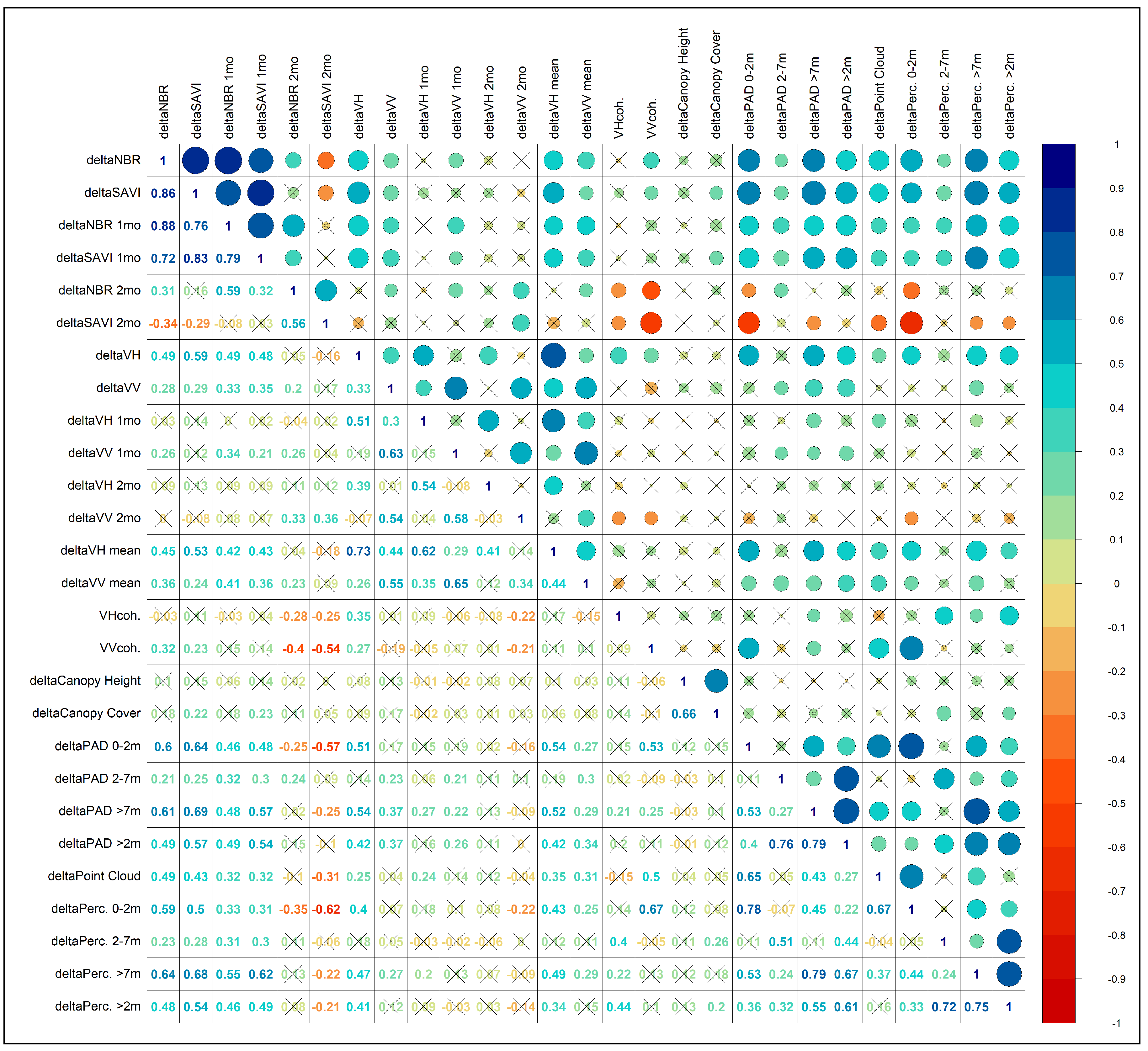
Once the final raster stack was generated, we performed a range of correlation tests using the Pearson method in R. The performance of each predictor was defined by their correlation coefficient r to the “deltaNBR” analysis, which is the established benchmark for the identification of burnt areas and their burn severities [45,46].
3. Results
3.1. Sensitivity of Optical and Sar Satellite Indices to Burn Severity
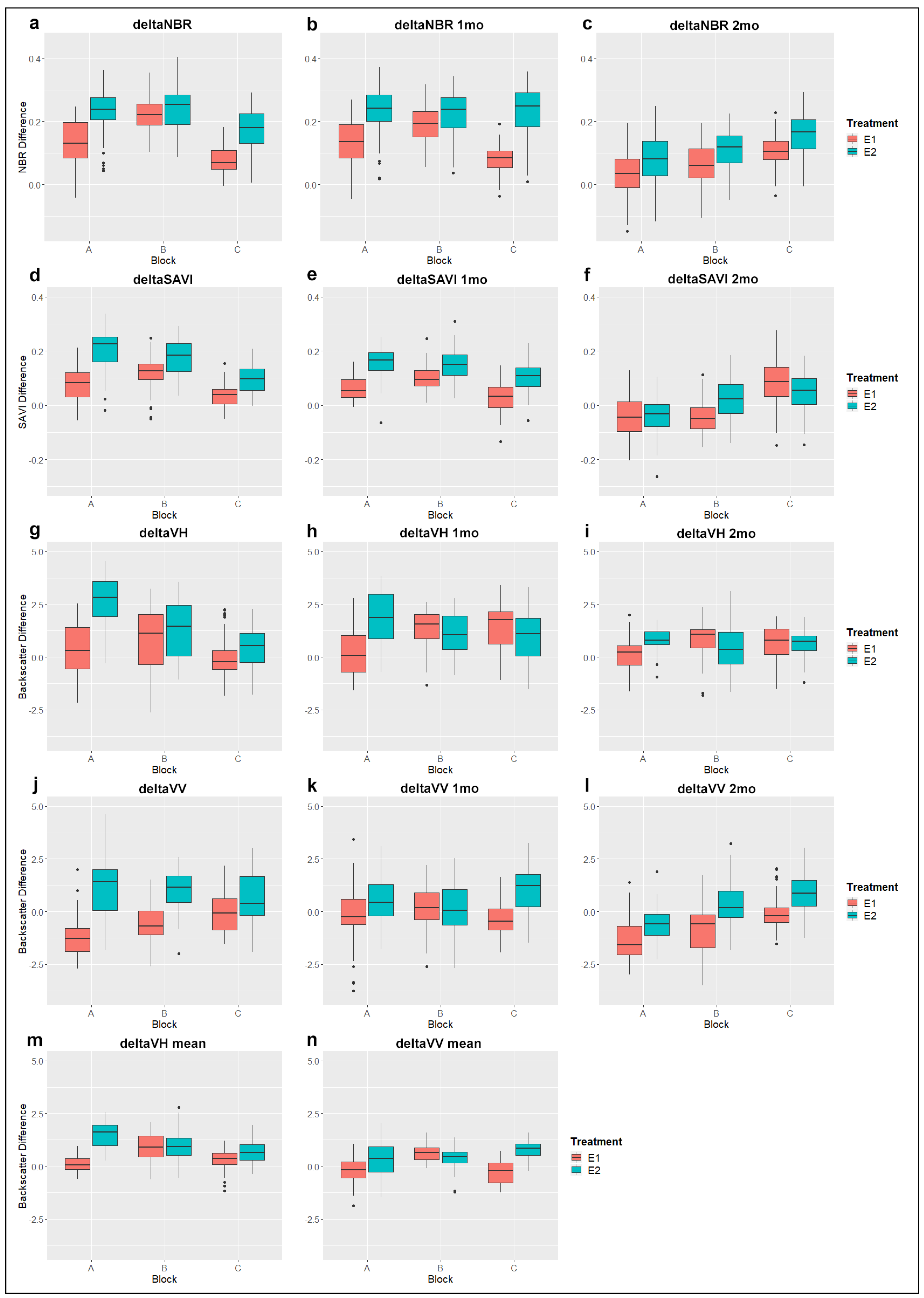
The “deltaNBR” and “deltaSAVI” indices that we derived from Sentinel-2 detected the experimental fire event and suggested that burn severity was higher within the E2 plots than the E1 plots (Figure 3). Fire effects were generally most pronounced immediately after the fire, with pre- and post-event differences diminishing after one and two month intervals, with the exception of “deltaSAVI” in plot E1 of block C (Figure 3f). While both optical indices “deltaNBR 1mo” and “deltaSAVI 1mo” still showed strong correlation (r = 0.88 and 0.72) with “deltaNBR”, analysis two months after the fire event showed weaker correlation coefficients, with “deltaSAVI 2mo” being negatively correlated (r = 0.31 and −0.34 for “deltaNBR 2mo” and “deltaSAVI 2mo” respectively) (Figure 4). The highest “deltaNBR” value derived from the pre- and post-fire analysis was 0.404 and is categorised as a moderate-low severity burn [47].
Our SAR-based results closely mirrored those from the optical satellite data. Both “deltaVH” and “deltaVV” calculations revealed greater differences and therefore higher burn severities for the E2 plots. “deltaVH” was most sensitive to the post-fire changes out of all the SAR predictors (Figure 3).
Additionally, both “deltaVH mean” and “deltaVV mean” backscatter difference also indicated higher burn severities for the E2 plots with the exception of “deltaVV mean”, which showed higher differences in plot E1 of Block B (Figure 3n). Creating the mean backscatter from five scenes improved the correlation coefficient slightly in the case of the VV data (r = 0.36 compared to 0.28 for “deltaVV”), but it did not improve the correlation results for the VH data.
Exploring trends over longer time-periods, higher values of “deltaVH 1mo” and “deltaVH 2mo” suggested that E1 plots of block B and C had higher burn severities, while “deltaVV 1mo” and “deltaVV 2mo” indicated higher burn severities for the E2 plots (with the exception of plot E1 in block B for the “deltaVV 1mo” predictor). That said, for both polarisations the correlation with “deltaNBR” became weaker as the time period following the fire increased (Figure 3 and Figure 4).
VV coherence information was more sensitive to the fire effects than VH coherence (r = 0.32 vs. −0.03); however, visual inspection revealed no clear identification of the actual burnt areas for both predictors.
3.2. Ground Validation of Fire Effects from Repeat TLS
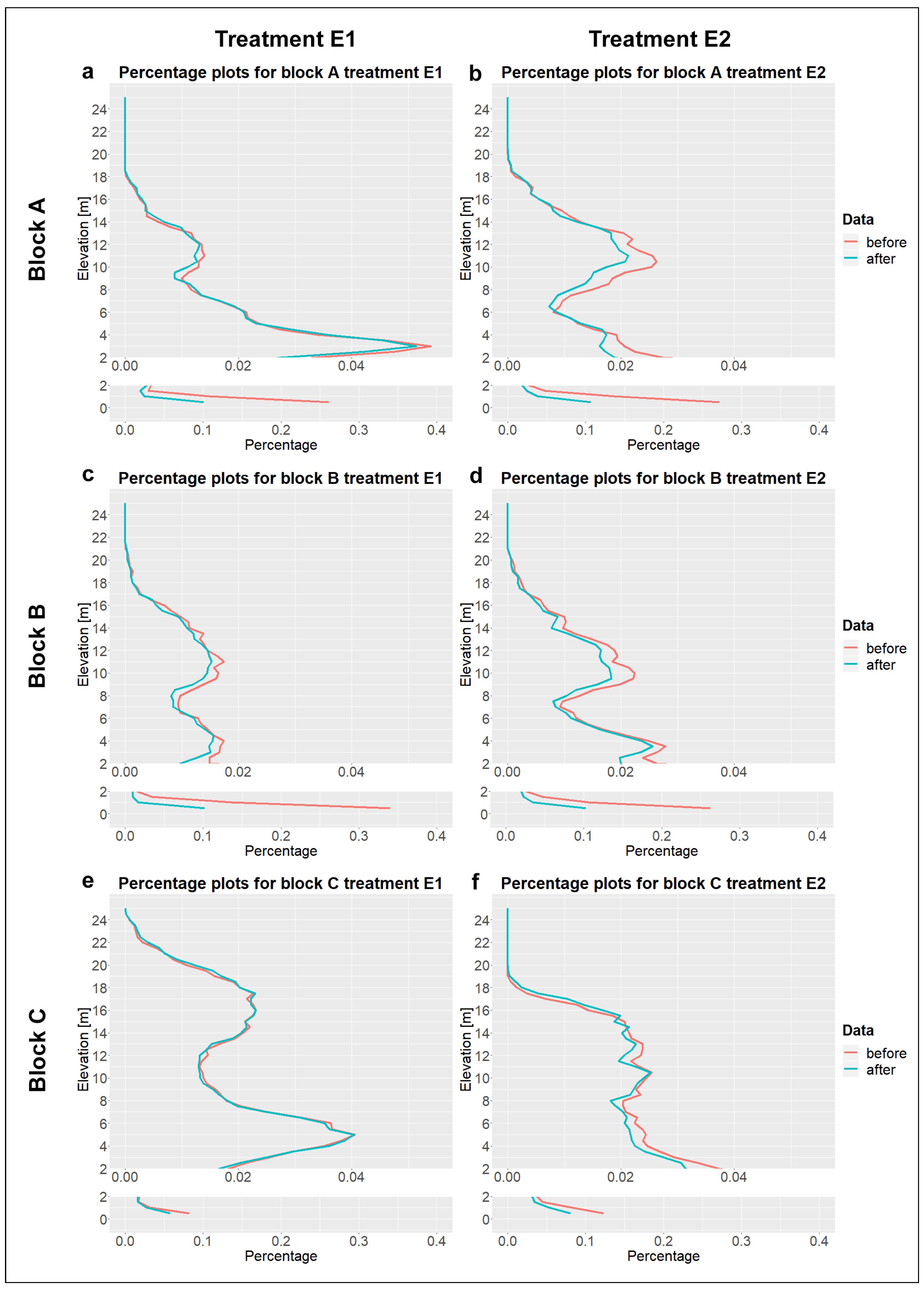
Analysing the difference between pre- and post-fire TLS data showed a general reduction in canopy resulting from the fires, but the magnitude of these effects differs among treatments and experimental blocks. Figure 5 visualizes the mean pre- and post-fire percentage profiles for each plot. The post-fire profiles show overall lower percentage numbers compared to the pre-fire profiles. Strongest differences between the before and after measurements are visible in the ground layer (0–2 m). Furthermore, differences between the percentage profiles are generally more pronounced for the E2 plots compared to the E1 treatment. Smallest changes were observed for plot E1 in block C (Figure 5e), while biggest changes can be seen within the ground layer (0–2 m) of plot E1 in block B (Figure 5c).
Pre- and post-fire TLS metrics showed significant correlations to both “deltaNBR” and “deltaSAVI” calculations, with “deltaCanopy Height” and “deltaCanopy Cover” being the only exceptions (Figure 4).
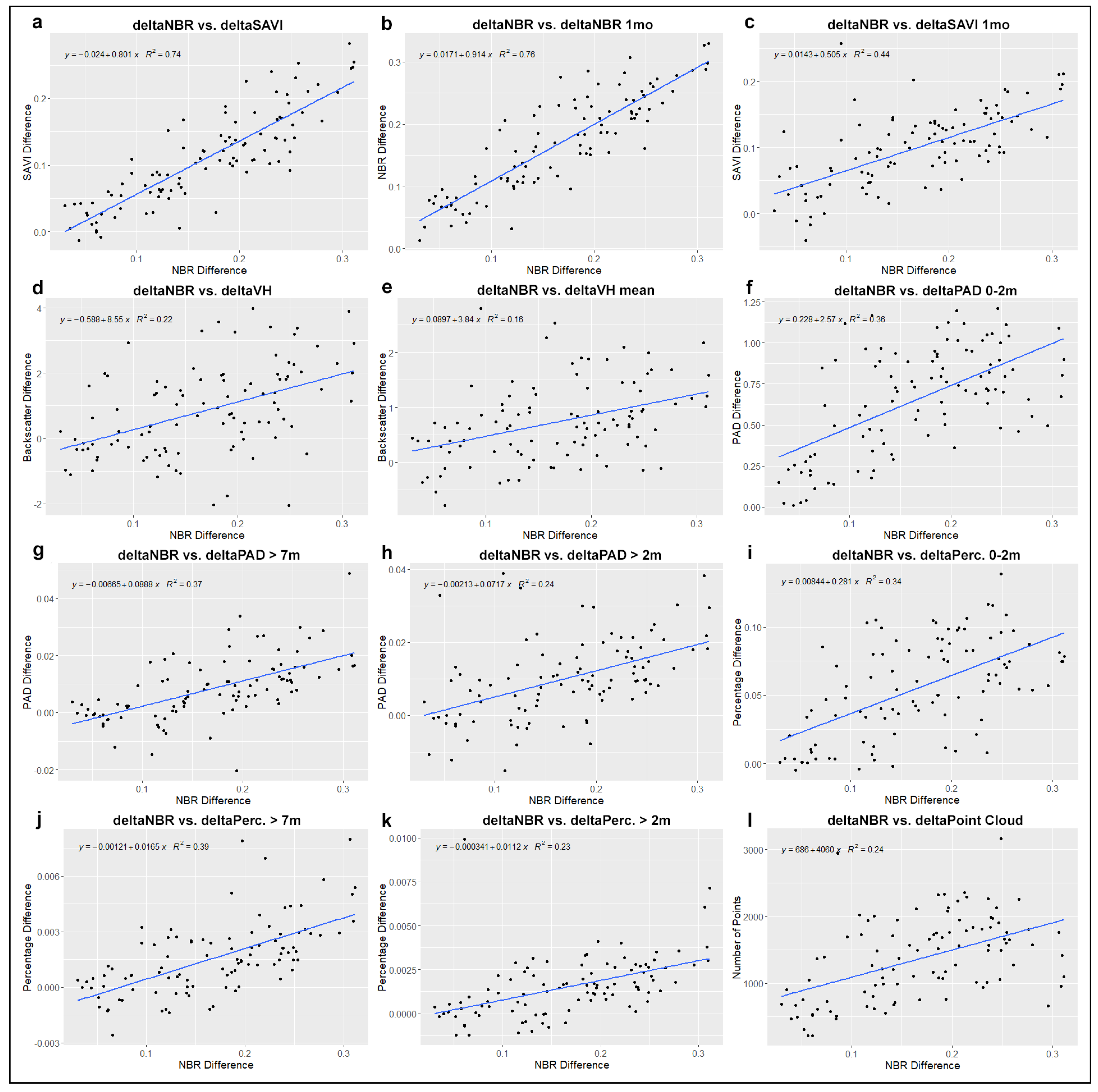
Comparing the PAD and percentage results, in both cases strongest correlation could be achieved with mean difference values derived from the ground layer (0–2 m) and the upper layers (>7 m). Mean difference values from 2–7 m performed the worst for both PAD and percentage difference. Mean difference values between the PAD and percentage approach were similar for all height bins, with the “deltaPerc.” values generating overall slightly higher correlation coefficients than “deltaNBR” (Figure 4). Scatterplots between “deltaNBR” and the best performing predictors per data type are visualized in Figure 6.
Canopy height and canopy cover difference were only weakly correlated with “deltaNBR” (r = 0.1 for canopy height and 0.18 for canopy cover), whereas the voxel analysis derived from the cloud-to-cloud difference predictor produced a correlation score of 0.49.
E2 plots featured higher volume losses in blocks A and C compared to the E1 plots within the same block. The least amount of lost biomass was observed for plot E1 in block C. In contrast to the other two blocks, most volume got lost in the E1 plot of block B which also features the highest volume loss out of all plots (Table 1).
4. Discussion
4.1. Sensitivity of C-Band Sar and Optical Imagery to Fire-Induced Change in Tropical Savannas
Our analysis of Sentinel-2 multi-spectral imagery showed that “deltaNBR” and “deltaSAVI”, which were strongly correlated with each other, were sensitive to the vegetational damage caused by the experimental fires at our study site. These indices have been shown to be useful indicators of burn severities around the globe [45,46,48], and as such, we used “deltaNBR” as the benchmark against which to evaluate the SAR results. Previous studies in other ecosystems have shown that the inclusion of SAR data can lead to improvements of estimations for burn severity mapping [49,50]. Our results corroborate this in tropical savanna landscapes, showing the strongest correlation between “deltaNBR” and SAR data for “deltaVH”. Our results build upon findings in African tropical forests [19] and savannas [51] which have also explored SAR backscatter differences following fires, but our results show the ability to move beyond straight detection and to retrieve information on severity.
Overall strongest correlations out of all SAR predictors were generated by using a VH backscatter scene directly after the fire (“deltaVH”) as well as by utilising mean backscatter data derived from five scenes after the fire. Analysis using single SAR scenes one and two months after the fire event resulted in significantly reduced correlation scores (Figure 4) and less consistent plot level severity analysis (Figure 3). Even though the “deltaVH mean” predictor also includes images that were acquired one and two months after the fire event, by calculating the mean value, a reduction of speckle noise was achieved which resulted in a higher signal to noise ratio. Therefore, correlation results of the “deltaVH mean” predictor were higher compared to using a single scene one and two months later.
Optical images collected one month after the fire event still showed strong correlations to the “deltaNBR” analysis from immediately after the fire event. Therefore, in case of cloud cover and other inclement weather conditions that could negatively influence the optical satellite imagery analysis, imagery acquired as long as one month after the fire event can still be used for burn severity assessment. In contrast to that, “deltaNBR” and “deltaSAVI” derived from imagery two months after the burning event led to significantly lower correlation values. Moreover, “deltaSAVI 2mo” showed a different trend for one of the blocks and a negative correlation coefficient to “deltaNBR”. Changes in soil and vegetation water content that occur as the dry season progresses become a major noise factor for identifying burning severities based on optical data. Said uncertainty increases with larger temporal differences and cannot completely be adjusted by using a mean general background trend within the Australian tropical savanna. Also, vegetational rehabilitation in the form of greening after the fire event represents another noise factor, which becomes increasingly difficult to adjust with an increasing temporal difference.
While other studies have shown a successful use of coherence analysis for burn scar mapping, e.g., Martinis et al. (2017) [50], our coherence analysis did not add value for burn severity quantification compared to the backscatter difference, with VH coherence showing especially low correlation. A moderate use of noise reduction in the form of small moving window sizes for multilooking and the leftover speckle noise after filtering could be the reason for that. However, as mentioned in the Methods section, we used moderate processing steps to keep as much detail and information as possible due to the small area of study size.
4.2. Ground Validation of Fire Effects with TLS
In this study, we used pre- and post-fire TLS to assess the impact of the fire event on vegetation structure. The vertical foliage profiles analysis of the TLS data showed that the E2 plots generally lost more plant volume in the fires than the E1 plots but that the magnitude did vary across the experiment site. Plot E1 in block C stands out by revealing very little difference in percentage profiles before and after the fire (Figure 5). The experimental fire in said plot did not completely burn through the whole plot and, therefore, caused comparatively little structural change. This is also reflected in the occupied volume reduction as seen in Table 1, which is lowest for plot E1 in block C out of all plots.
PAD and percentage analysis showed highest correlation values for both the ground layer (0–2 m) as well as for predictors including the canopy layer (>2 m and >7 m). This suggests higher fire-related structural changes within the ground and canopy layers compared to the middle layer (2–7 m), which generated lowest correlation values for both the PAD and the percentage analysis. These observations are also reflected in the before and after profile analyses (Figure 5). This could be explained by the burnt grasses and bushes within the ground layer as well as by the loss of scorched leaves of the canopy layer. The middle layer in contrast features predominantly stems. Structural changes within this height range do not necessarily relate with the spectral response of satellite data as well as changes in the canopy and ground layer.
While other studies successfully demonstrated the use of LiDAR-derived changes in canopy height and canopy cover for estimations related to biomass combustion and therefore burn severity [45,52], differences in canopy height and canopy cover in this study responded relatively weakly compared to other TLS metrics. We consider this to be a function of the savanna vegetation type, which is largely resilient to fire and does not shrink in height after the fire but rather thins out due to loss of leaves (unless a whole tree is toppled). Most of the volume loss that we measured with the repeat TLS was from the ground level (0–2 m). Compared to the volume loss at ground level, changes in the upper vegetation layers were more subtle (Figure 5), and the low-severity and moderate-low severity burns, as categorised by “deltaNBR”, were potentially not intense enough to impart upper canopy changes.
Results based on indices derived from Sentinel-2 optical satellite imagery suggest overall higher burn severities for plots which are burnt every second year compared to the more frequently burnt plots. The same results were generated during a long-term observation (2004–2013) [6]. Higher burn severities for the two-year treatment could be explained by a higher fuel development in the form of shrubs and grasses compared the yearly burnt plots. For land management, these results suggest overall lower burn severities with higher frequency burns. Volume loss estimation based on repeat TLS data was largely supportive of this, with the exception of the E1 plot in block B (Table 1). Profile analysis hereby revealed the strongest biomass loss between 0–2 m elevation out of all plots (Figure 5c). Satellite remote-sensing data is heavily influenced by changes in the canopy and is also restricted by its spatial resolution, while TLS data with its ability to analyse structural differences below the canopy in combination with its high point density is able to pick up small-scale changes that are less likely detectable from space. Biggest differences in point numbers before and after the fire were present between 0–2 m, which suggests highest biomass loss within the ground layer. Since TLS data is not restricted by the canopy in its ability to detect changes on the ground, it provides a powerful tool to understand vegetation structural changes under canopies that might be hidden from the air or from space.
4.3. Limitations and Future Directions
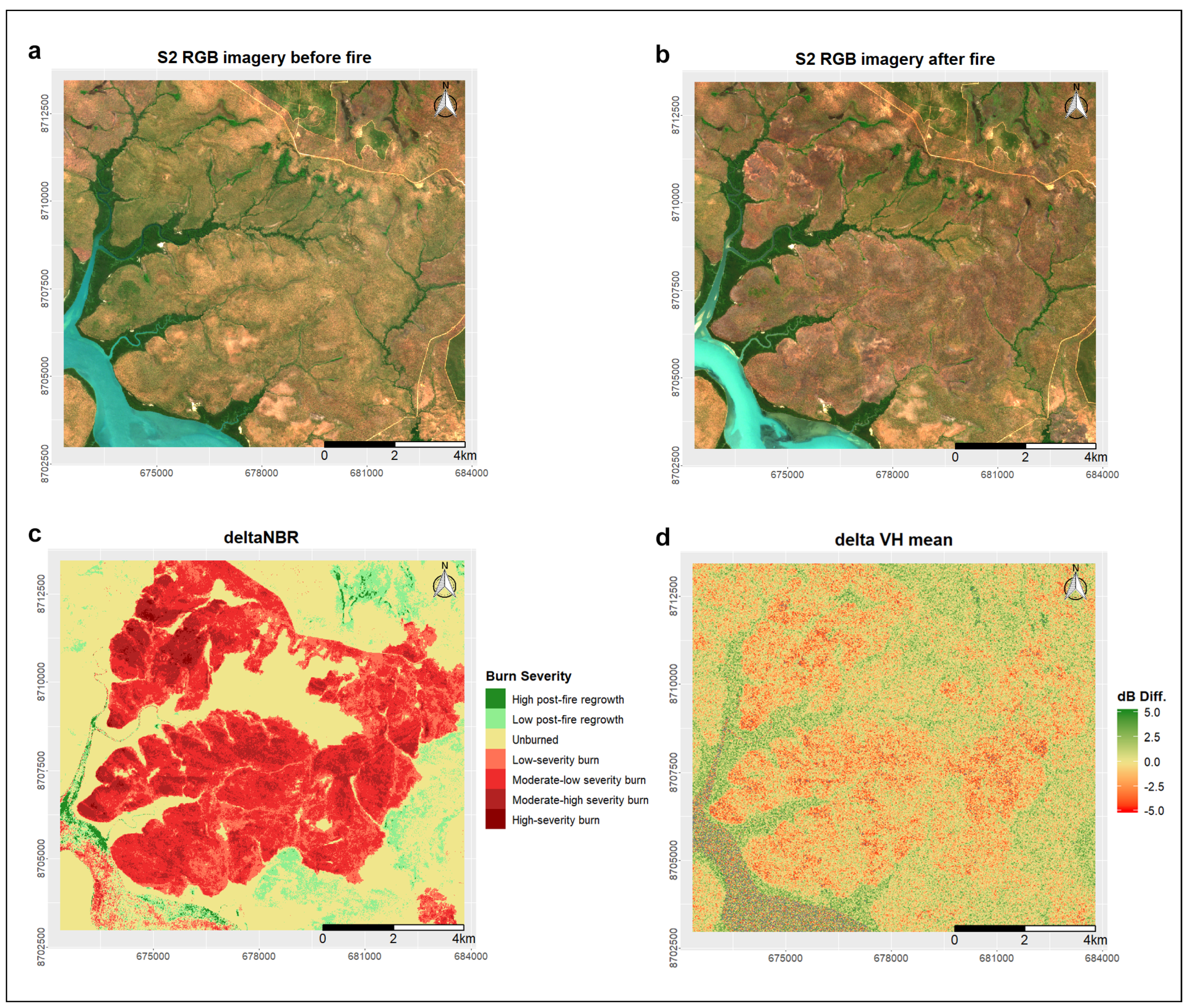
The primary limitation of our study was the relatively small size of the experimental fire plots (1 ha), which restricted the number of satellite pixels that could be assessed on a per treatment basis. Backscatter difference of SAR data which is based on structural changes and moisture content is expected to vary as a function of these differences. With a high loss of vegetated material, surface scattering increases relative to the volume scattering [53,54]. With low burn severities and therefore relatively small structural changes, it becomes increasingly difficult to detect and quantify such changes. Furthermore, a larger area of interest would result in more pixels that can be compared, which not only would make the analysismore representative but also would allow for more aggressive noise-reduction approaches for reducing the speckle effect in the case of SAR data. An example of a larger-scale fire detection using SAR backscatter difference can be seen in Figure 7. Areas of higher “deltaNBR” burn severities (Figure 7c) feature also stronger backscatter differences (Figure 7d).
Each of the three data sets used in this study is characterised by distinct advantages and disadvantages for detecting burn severity. Optical data derived from Sentinel-2 features a relatively high spatial resolution of up to 10 m (depending on the used spectral bands), a revisit time of 5 days (when combining both Sentinel-2A and Sentinel-2B), as well as a wide swath width of 250 km [27]. However, the usage of optical data is highly limited by the present weather condition and fire-related smoke screens, which may lead to a time-gap between the actual fire and available surface information. As seen in this study, increasing the temporal distance between the before and after fire images also introduces higher uncertainties. Sentinel-1 C-band SAR data provides a similar spatial resolution (5 m by 20 m per pixel) and revisit time (6 days when combining both Sentinel-1A and Sentinel-1B), together with a slightly larger swath width of 290 km [32]. The major advantage of SAR lies thereby in its weather-independent application, which allows for a full exploitation of its high temporal resolution. On the other hand, speckle-induced noise makes backscatter difference analysis challenging, especially for lower burn severities and related minor structural changes. Variability in moisture contents due to rain can further impair the quality of SAR analysis.
TLS data provides highly detailed information about structural changes and biomass loss estimations by creating high-density point clouds. Limitations of the TLS approach include increased occlusion of the laser beam in denser vegetation and the relatively small area of coverage compared to satellite imagery. However, in open woodland savanna, the TLS approach can suitably capture many hectares across larger experimental sites [55]. Lastly, wind-related movements of branches and leaves is an important uncertainty factor that needs to be considered. A detailed overview of the used data and their specifications can be found in Table 2.
Moreover, existing burn severity classifications based on the NBR are unlikely to apply directly in tropical savanna landscapes. In contrast to other forest types, fire is common in savanna landscapes and trees feature fire adaptations such thick bark and large underground storage organs [56]. The actual burn severity is likely to differ from the NBR-based severity classification, depending on the land cover type. Hence, high NBR burn severity relationships do not necessarily correspond to high delta NBR burn severities in tropical savanna landscapes. As also suggested by Lentile et al. (2006), more research is needed to develop direct “deltaNBR” severity classifications across a variety of fire regimes and vegetation biomes, including savanna landscapes [57].
5. Conclusions
Satellite-based SAR data proved sensitive to burn severity in our tropical savanna study area, indicating higher severities in areas that were burnt every second year compared to annually burnt plots. This pattern likely reflects higher fuel load development in the grass and shrub layer, and the SAR findings mirrored results obtained from delta NBR mapping with optical satellites. Plot-scale change metrics were in good agreement with actual structural changes on the ground, as determined from volumetric and foliage profile reductions that we quantified with repeat terrestrial laser scanning (TLS).
The optical indices “deltaNBR” and “deltaSAVI” derived from Sentinel-2 imagery provided a quick, intuitive, and operational means of estimating burn severity. C-band VH backscatter data performed the best of the SAR products we analysed. While SAR data showed similar results on a plot level compared to optical data, for a pixel-based comparison, a larger area of study, higher burn severities, and more aggressive noise reduction are recommended. Lastly, the temporal difference between the before and after fire scenes should be kept as small as possible for the best results. While optical data one month after the fire event can still be feasible for burn severity analysis, in the case of SAR data, imagery captured either directly after the fire or the use of mean backscatter data from five scenes is recommended.
This study highlights the potential of C-band SAR data to contribute to burn severity mapping in tropical savannas. In addition to optical satellite data, we used TLS measurements to validate our findings, which to our knowledge has not been done before in the context of burn severity quantification. SAR data contributed valuable information which was correlated with optical observations and TLS measurements. For increasing the information density and for mitigating limitations of optical data such as clouds, the use of SAR data as an additional predictor can be recommended for similar studies.
Author Contributions
Conceptualization, S.R.L.; methodology, M.B.P. and S.R.L.; software, M.B.P. and S.R.L.; validation, M.B.P.; formal analysis, M.B.P.; investigation, M.B.P. and S.R.L.; resources, M.B.P. and S.R.L.; data curation, M.B.P. and S.R.L.; writing—original draft preparation, M.B.P.; writing—review and editing, S.R.L.; visualization, M.B.P.; supervision, S.R.L.; project administration, S.R.L.; funding acquisition, M.B.P. and S.R.L. All authors have read and agree to the published version of the manuscript.
Funding
This project was supported by funding from the CSIRO and the Australian Government’s National Environmental Science Programme (NESP). This publication was funded by the German Research Foundation (DFG) and the University of Wuerzburg in the funding programme Open Access Publishing.
Acknowledgments
We acknowledge the Northern Territory Government and the Territory Wildlife Park for establishing and maintaining the long-term fire experimental site. We thank A. Sullivan and two anonymous reviewers for their valuable comments on this manuscript.
Conflicts of Interest
The authors declare no conflict of interest.
References
- Bond, W.J.; Keeley, J.E. Fire as a global ‘herbivore’: The ecology and evolution of flammable ecosystems. Trends Ecol. Evol. 2005, 20, 387–394. [Google Scholar] [CrossRef] [PubMed]
- Beringer, J.; Hutley, L.B.; Abramson, D.; Arndt, S.K.; Briggs, P.; Bristow, M.; Canadell, J.G.; Cernusak, L.A.; Eamus, D.; Edwards, A.C.; et al. Fire in Australian savannas: From leaf to landscape. Glob. Chang. Biol. 2015, 21, 62–81. [Google Scholar] [CrossRef] [PubMed] [Green Version]
- Australian Government—Bureau of Meteorology. Climate Statistics for Australian Locations. 2019. Available online: http://www.bom.gov.au/climate/averages/tables/cw_014015.shtml (accessed on 5 January 2019).
- Sturman, A.P.; Tapper, N.J. Weather and Climate of Australia and New Zealand, 2nd ed.; Oxford University Press: Melbourne, VIC, Australia, 2006. [Google Scholar]
- Beck, H.E.; Zimmermann, N.E.; McVicar, T.R.; Vergopolan, N.; Berg, A.; Wood, E.F. Present and future Köppen-Geiger climate classification maps at 1-km resolution. Sci. Data 2018, 5, 180214. [Google Scholar] [CrossRef] [PubMed] [Green Version]
- Levick, S.R.; Richards, A.E.; Cook, G.D.; Schatz, J.; Guderle, M.; Williams, R.J.; Subedi, P.; Trumbore, S.E.; Andersen, A.N. Rapid response of habitat structure and aboveground carbon storage to altered fire regimes in tropical savanna. Biogeosciences 2019, 1. [Google Scholar] [CrossRef] [Green Version]
- Australian Government—Department of the Environment and Energy. Climate Solutions Fund—Emissions Reduction Fund. Available online: https://www.environment.gov.au/climate-change/government/emissions-reduction-fund (accessed on 30 November 2019).
- Perry, J.J.; Sinclair, M.; Wikmunea, H.; Wolmby, S.; Martin, D.; Martin, B. The divergence of traditional Aboriginal and contemporary fire management practices on Wik traditional lands, Cape York Peninsula, Northern Australia. Ecol. Manag. Restor. 2018, 19, 24–31. [Google Scholar] [CrossRef] [Green Version]
- Russell-Smith, J.; Murphy, B.P.; Meyer, C.M.; Cook, G.D.; Maier, S.; Edwards, A.C.; Schatz, J.; Brocklehurst, P. Improving estimates of savanna burning emissions for greenhouse accounting in northern Australia: Limitations, challenges, applications. Int. J. Wildl. Fire 2009, 18, 1–18. [Google Scholar] [CrossRef]
- Tingley, M.W.; Ruiz-Gutiérrez, V.; Wilkerson, R.L.; Howell, C.A.; Siegel, R.B. Pyrodiversity promotes avian diversity over the decade following forest fire. Proc. R. Soc. B Biol. Sci. 2016, 283, 20161703. [Google Scholar] [CrossRef] [Green Version]
- Ponisio, L.C.; Wilkin, K.; M’gonigle, L.K.; Kulhanek, K.; Cook, L.; Thorp, R.; Griswold, T.; Kremen, C. Pyrodiversity begets plant—Pollinator community diversity. Glob. Chang. Biol. 2016, 22, 1794–1808. [Google Scholar] [CrossRef] [Green Version]
- Bradstock, R.; Auld, T. Soil temperatures during experimental bushfires in relation to fire intensity: Consequences for legume germination and fire management in south-eastern Australia. J. Appl. Ecol. 1995, 32, 76–84. [Google Scholar] [CrossRef]
- Penman, T.; Binns, D.; Kavanagh, R. Burning for Biodiversity or Burning the Biodiversity? In Proceedings of the Australasian Fire Association Council Conference, Hobart, Australia, 2007; Available online: http://proceedings. com. au/tassiefire/papers pdf/fri penman.pdf (accessed on 30 November 2019).
- Corey, B.; Andersen, A.N.; Legge, S.; Woinarski, J.C.Z.; Radford, I.J.; Perry, J.J. Better biodiversity accounting is needed to prevent bioperversity and maximize co-benefits from savanna burning. Conserv. Lett. 2019, e12685. [Google Scholar] [CrossRef]
- Hudak, A.; Brockett, B. Mapping fire scars in a southern African savannah using Landsat imagery. Int. J. Remote Sens. 2004, 25, 3231–3243. [Google Scholar] [CrossRef]
- Archibald, S.; Nickless, A.; Govender, N.; Scholes, R.J.; Lehsten, V. Climate and the inter-annual variability of fire in southern Africa: A meta-analysis using long-term field data and satellite-derived burnt area data. Glob. Ecol. Biogeogr. 2010, 19, 794–809. [Google Scholar] [CrossRef]
- Maier, S.W.; Russell-Smith, J. Measuring and monitoring of contemporary fire regimes in Australia using satellite remote sensing. In Flammable Australia: Fire Regimes, Biodiversity and Ecosystems in a Changing World; CSIRO Publishing: Melbourne, VIC, Australia, 2012; pp. 79–95. [Google Scholar]
- Boschetti, L.; Roy, D.P.; Justice, C.O.; Humber, M.L. MODIS—Landsat fusion for large area 30 m burned area mapping. Remote Sens. Environ. 2015, 161, 27–42. [Google Scholar] [CrossRef]
- Verhegghen, A.; Eva, H.; Ceccherini, G.; Achard, F.; Gond, V.; Gourlet-Fleury, S.; Cerutti, P. The potential of Sentinel satellites for burnt area mapping and monitoring in the Congo Basin forests. Remote Sens. 2016, 8, 986. [Google Scholar] [CrossRef] [Green Version]
- Roy, D.P.; Boschetti, L.; Trigg, S.N. Remote sensing of fire severity: Assessing the performance of the normalized burn ratio. IEEE Geosci. Remote Sens. Lett. 2006, 3, 112–116. [Google Scholar] [CrossRef] [Green Version]
- Quintano, C.; Fernández-Manso, A.; Fernández-Manso, O. Combination of Landsat and Sentinel-2 MSI data for initial assessing of burn severity. Int. J. Appl. Earth Observ. Geoinf. 2018, 64, 221–225. [Google Scholar] [CrossRef]
- Jain, T.B.; Graham, R.T.; Pilliod, D.S. Tongue-tied: Confused meanings for common fire terminology can lead to fuels mismanagement. Wildfire 2004, 4, 22–26. [Google Scholar]
- Conard, S.G.; Sukhinin, A.I.; Stocks, B.J.; Cahoon, D.R.; Davidenko, E.P.; Ivanova, G.A. Determining effects of area burned and fire severity on carbon cycling and emissions in Siberia. Clim. Chang. 2002, 55, 197–211. [Google Scholar] [CrossRef]
- Miller, J.D.; Yool, S.R. Mapping forest post-fire canopy consumption in several overstory types using multi-temporal Landsat TM and ETM data. Remote Sens. Environ. 2002, 82, 481–496. [Google Scholar] [CrossRef]
- Richards, A.E.; Dathe, J.; Cook, G.D. Fire interacts with season to influence soil respiration in tropical savannas. Soil Biol. Biochem. 2012, 53, 90–98. [Google Scholar] [CrossRef]
- European Space Agency, European Union. Copernicus Open Access Hub. 2019. Available online: https://scihub.copernicus.eu/ (accessed on 5 January 2019).
- European Space Agency. Sentinel-2 User Handbook. 2015. Available online: https://sentinels.copernicus.eu/documents/247904/685211/Sentinel-2_User_Handbook (accessed on 5 January 2019).
- European Space Agency. Sen2Cor v2.5.5. Available online: http://step.esa.int/main/third-party-plugins-2/sen2cor/sen2cor_v2-5-5/ (accessed on 5 January 2019).
- Louis, J. Sentinel 2 MSI—Level 2A Product Definition. 2017. Available online: https://sentinel.esa.int/documents/247904/685211/S2+L2A+Product+Definition+Document/2c0f6d5f-60b5-48de-bc0d-e0f45ca06304 (accessed on 5 January 2019).
- Huete, A.R. A soil-adjusted vegetation index (SAVI). Remote Sens. Environ. 1988, 25, 295–309. [Google Scholar] [CrossRef]
- García, M.L.; Caselles, V. Mapping burns and natural reforestation using Thematic Mapper data. Geocarto Int. 1991, 6, 31–37. [Google Scholar] [CrossRef]
- ESA Communications. Sentinel-1 ESA’s Radar Observatory Mission for GMES Operational Services. 2012. Available online: http://esamultimedia.esa.int/multimedia/publications/SP-1322_1/ (accessed on 5 January 2019).
- European Space Agency. SNAP. Available online: https://step.esa.int/main/toolboxes/snap/ (accessed on 5 January 2019).
- Veci, L. Sentinel-1 Toolbox—TOPS Interferometry Tutorial. 2016. Available online: https://step.esa.int/docs/tutorials/S1TBX%20TOPSAR%20Interferometry%20with%20Sentinel-1%20Tutorial.pdf (accessed on 6 December 2019).
- Rapidlasso GmbH. LAStools. Available online: https://rapidlasso.com/lastools/ (accessed on 5 January 2019).
- Girardeau-Montaut, D. CloudCompare. Available online: https://www.danielgm.net/cc/ (accessed on 5 January 2019).
- R Core Team. R: A Language and Environment for Statistical Computing. Available online: https://www.R-project.org/ (accessed on 5 January 2019).
- Zhao, F.; Yang, X.; Schull, M.A.; Román-Colón, M.O.; Yao, T.; Wang, Z.; Zhang, Q.; Jupp, D.L.; Lovell, J.L.; Culvenor, D.S.; et al. Measuring effective leaf area index, foliage profile, and stand height in New England forest stands using a full-waveform ground-based lidar. Remote Sens. Environ. 2011, 115, 2954–2964. [Google Scholar] [CrossRef]
- Detto, M.; Asner, G.P.; Muller-Landau, H.C.; Sonnentag, O. Spatial variability in tropical forest leaf area density from multireturn lidar and modeling. J. Geophys. Res. Biogeosci. 2015, 120, 294–309. [Google Scholar] [CrossRef]
- Hosoi, F.; Omasa, K. Estimating vertical plant area density profile and growth parameters of a wheat canopy at different growth stages using three-dimensional portable lidar imaging. ISPRS J. Photogramm. Remote Sens. 2009, 64, 151–158. [Google Scholar] [CrossRef]
- Bouvier, M.; Durrieu, S.; Fournier, R.A.; Renaud, J.P. Generalizing predictive models of forest inventory attributes using an area-based approach with airborne LiDAR data. Remote Sens. Environ. 2015, 156, 322–334. [Google Scholar] [CrossRef]
- Électricité de France. Distances Computation. 2015. Available online: https://www.cloudcompare.org/doc/wiki/index.php?title=Distances_Computation (accessed on 5 January 2019).
- Yan, L.; Roy, D.; Li, Z.; Zhang, H.; Huang, H. Sentinel-2A multi-temporal misregistration characterization and an orbit-based sub-pixel registration methodology. Remote Sens. Environ. 2018, 215, 495–506. [Google Scholar] [CrossRef]
- Roy, D.P.; Wulder, M.; Loveland, T.R.; Woodcock, C.; Allen, R.; Anderson, M.; Helder, D.; Irons, J.; Johnson, D.; Kennedy, R.; et al. Landsat-8: Science and product vision for terrestrial global change research. Remote Sens. Environ. 2014, 145, 154–172. [Google Scholar] [CrossRef] [Green Version]
- McCarley, T.R.; Kolden, C.A.; Vaillant, N.M.; Hudak, A.T.; Smith, A.M.; Wing, B.M.; Kellogg, B.S.; Kreitler, J. Multi-temporal LiDAR and Landsat quantification of fire-induced changes to forest structure. Remote Sens. Environ. 2017, 191, 419–432. [Google Scholar] [CrossRef] [Green Version]
- Hoy, E.E.; French, N.H.; Turetsky, M.R.; Trigg, S.N.; Kasischke, E.S. Evaluating the potential of Landsat TM/ETM+ imagery for assessing fire severity in Alaskan black spruce forests. Int. J. Wildl. Fire 2008, 17, 500–514. [Google Scholar] [CrossRef]
- Humboldt State University. Normalized Burn Ratio. 2015. Available online: http://gsp.humboldt.edu/olm_2015/Courses/GSP_216_Online/lesson5-1/NBR.html (accessed on 5 January 2019).
- Escuin, S.; Navarro, R.; Fernandez, P. Fire severity assessment by using NBR (Normalized Burn Ratio) and NDVI (Normalized Difference Vegetation Index) derived from LANDSAT TM/ETM images. Int. J. Remote Sens. 2008, 29, 1053–1073. [Google Scholar] [CrossRef]
- Tanase, M.A.; Kennedy, R.; Aponte, C. Fire severity estimation from space: A comparison of active and passive sensors and their synergy for different forest types. Int. J. Wildl. Fire 2015, 24, 1062–1075. [Google Scholar] [CrossRef]
- Martinis, S.; Caspard, M.; Plank, S.; Clandillon, S.; Haouet, S. Mapping burn scars, fire severity and soil erosion susceptibility in Southern France using multisensoral satellite data. In Proceedings of the 2017 IEEE International Geoscience and Remote Sensing Symposium (IGARSS), Fort Worth, TX, USA, 23–28 July 2017; pp. 1099–1102. [Google Scholar]
- Mathieu, R.; Main, R.; Roy, D.; Naidoo, L.; Yang, H. Detection of burned areas in southern African savannahs using time series of C-band sentinel-1 data. In Proceedings of the International Geoscience and Remote Sensing Symposium (IGARSS), Valencia, Spain, 22–27 July 2018; pp. 5337–5339. [Google Scholar] [CrossRef]
- Wang, C.; Glenn, N.F. Estimation of fire severity using pre-and post-fire LiDAR data in sagebrush steppe rangelands. Int. J. Wildl. Fire 2009, 18, 848–856. [Google Scholar] [CrossRef] [Green Version]
- Kalogirou, V.; Ferrazzoli, P.; Della Vecchia, A.; Foumelis, M. On the SAR backscatter of burned forests: A model-based study in C-band, over burned pine canopies. IEEE Trans. Geosci. Remote Sens. 2014, 52, 6205–6215. [Google Scholar] [CrossRef]
- Kasischke, E.; Bourgeau-Chavez, L.; French, N.; Harrell, P.; Christensen, N., Jr. Initial observations on using SAR to monitor wildfire scars in boreal forests. Int. J. Remote Sens. 1992, 13, 3495–3501. [Google Scholar] [CrossRef]
- Singh, J.; Levick, S.R.; Guderle, M.; Schmullius, C.; Trumbore, S.E. Variability in fire-induced change to vegetation physiognomy and biomass in semi-arid savanna. Ecosphere 2018, 9, e02514. [Google Scholar] [CrossRef] [Green Version]
- Maurin, O.; Davies, T.J.; Burrows, J.E.; Daru, B.H.; Yessoufou, K.; Muasya, A.M.; Van der Bank, M.; Bond, W.J. Savanna fire and the origins of the ‘underground forests’ of A frica. New Phytol. 2014, 204, 201–214. [Google Scholar] [CrossRef] [Green Version]
- Lentile, L.B.; Holden, Z.A.; Smith, A.M.; Falkowski, M.J.; Hudak, A.T.; Morgan, P.; Lewis, S.A.; Gessler, P.E.; Benson, N.C. Remote sensing techniques to assess active fire characteristics and post-fire effects. Int. J. Wildl. Fire 2006, 15, 319–345. [Google Scholar] [CrossRef]
- RIEGL. RIEGL VZ-2000i. Available online: http://www.riegl.com/nc/products/terrestrial-scanning/produktdetail/product/scanner/58/ (accessed on 30 November 2019).
Figure 1.
Area of study ∼50 km south of Darwin: 18 plots are divided into three blocks, each block consisting of six plots with a different fire treatment per plot. An area of similar vegetation type was defined to analyse background trends along the western edge of the plots. Fire events analysed in this study were conducted on plots E1 and E2 within each block.

Figure 2.
Terrestrial Laser Scanning (TLS) point clouds of plot E2 in block B after de-noising and thinning, together with TLS-derived canopy height rasters: LiDAR measurements shortly before (a,b) and shortly after (c,d) the experimental fires, as well as the respective differences (e,f) are displayed.

Figure 3.
Sensitivity of optical (a–f) and Synthetic Aperture Radar (SAR) (g–n) indices to fire treatment effects on savanna vegetation visualized by box plots: The box and whiskers of each box plot are quartiles, with the band inside each box being the median value. Outliers are displayed as points. Based on the median values of each box plot, the majority of the predictors suggest higher burn severities for the E2 plots compared to the E1 plots. An increasing temporal difference between the before and after fire scenes lead to less consistent results among the data sets.

Figure 4.
Correlogram displaying the correlation magnitude and direction between all predictors: Numbers range from −1 to 1, which is also visualized by the circle sizes. The colour coding further displays the degree of correlation as well as the direction (positive = blueish; negative = reddish). Central to this study is the correlation between “deltaNBR” (first column) and all other predictors. Values which are crossed out (X) are not statistically significant (p > 0.05).

Figure 5.
Mean vertical foliage percentage profiles before and after the fire event for each treatment (a,c,e = burning every year; b,d,f = burning every second year): Profiles were generated using thinned TLS data. For the sake of clarity, each plot has been divided into two parts with different x-axis scales. Profiles start at 0.5 m with a bin height of 0.5 m. Greatest differences between the before and after plots can be observed in elevations between 0–2 m. Percentage values range between 0 and 1, with 1 = 100%.

Figure 6.
Relationships visualized by scatter plots between “deltaNBR” and other change indices derived from optical (a–c), SAR (d,e), and TLS data (f–l): Vertical foliage profiles from both the canopy layer and the ground layer performed best within the TLS predictors, while “deltaVH” backscatter showed the strongest correlation within the SAR predictors.

Figure 7.
Example of larger-scale detection of savanna burn scar extent on the Tiwi Islands with optical and SAR sensors: Optical images before (a) and after (b) the fire are visualized. High burn severities as classified by “deltaNBR” (c) also stand out in the mean delta VH SAR image (d). Preprocessing of the shown radar image included thermal noise removal, radiometric calibration, terrain correction, and a conversion to dB. No speckle filtering was applied to the visualised SAR scene.


Table 1.
Occupied volume reduction per plot (m).
| Block: | Block A | Block B | Block C | |||
|---|---|---|---|---|---|---|
| Fire Treatment: | E1 | E2 | E1 | E2 | E1 | E2 |
| Lost biomass volume m: | 342.440 | 392.064 | 452.528 | 391.440 | 222.104 | 386.656 |
Table 2.
Specifications of the three different data origins Sentinel-2 multispectral optical imagery, Sentinel-1 C-band SAR imagery, and RIEGL-VZ2000 TLS data (adapted from [27,32,58]).
| Data origin: | Sentinel-2 | Sentinel-1 | RIEGL-VZ2000 |
|---|---|---|---|
| Data type: | Optical (multispectral) | C-band SAR (Interferometric Wide Swath “IW” Mode) | LiDAR (TLS) |
| Spatial resolution(s): | Pixel sizes: 10 m, 20 m and 60 m | Pixel size: 5 m by 20 m | Point density: sub-centimeter level (Depending on distance to sensor) |
| Spatial coverage: | Swath width: 250 km | Swath width: 290 km | Radial range: up to 2500 m |
| Temporal resolution: | At equator level: 10 days (one satellite) 5 days (two satellites) | At equator level: 12 days (one satellite) 6 days (two satellites) | User-dependent |
| Day/night application: | Not possible | Possible | Possible |
| Information about vegetation structure: | None | Limited | Detailed |
| Weather dependency: | Strongly dependent | Largely independent | Strongly dependent |
| Study area accessibility: | Independent | Independent | Strongly dependent |
© 2019 by the authors. Licensee MDPI, Basel, Switzerland. This article is an open access article distributed under the terms and conditions of the Creative Commons Attribution (CC BY) license (http://creativecommons.org/licenses/by/4.0/).
Share and Cite
MDPI and ACS Style
Philipp, M.B.; Levick, S.R. Exploring the Potential of C-Band SAR in Contributing to Burn Severity Mapping in Tropical Savanna. Remote Sens. 2020, 12, 49. https://0-doi-org.brum.beds.ac.uk/10.3390/rs12010049
AMA Style
Philipp MB, Levick SR. Exploring the Potential of C-Band SAR in Contributing to Burn Severity Mapping in Tropical Savanna. Remote Sensing. 2020; 12(1):49. https://0-doi-org.brum.beds.ac.uk/10.3390/rs12010049
Chicago/Turabian StylePhilipp, Marius B., and Shaun R. Levick. 2020. "Exploring the Potential of C-Band SAR in Contributing to Burn Severity Mapping in Tropical Savanna" Remote Sensing 12, no. 1: 49. https://0-doi-org.brum.beds.ac.uk/10.3390/rs12010049
Note that from the first issue of 2016, this journal uses article numbers instead of page numbers. See further details here.