The 2014 Mw 6.1 Ludian Earthquake: The Application of RADARSAT-2 SAR Interferometry and GPS for this Conjugated Ruptured Event


Abstract
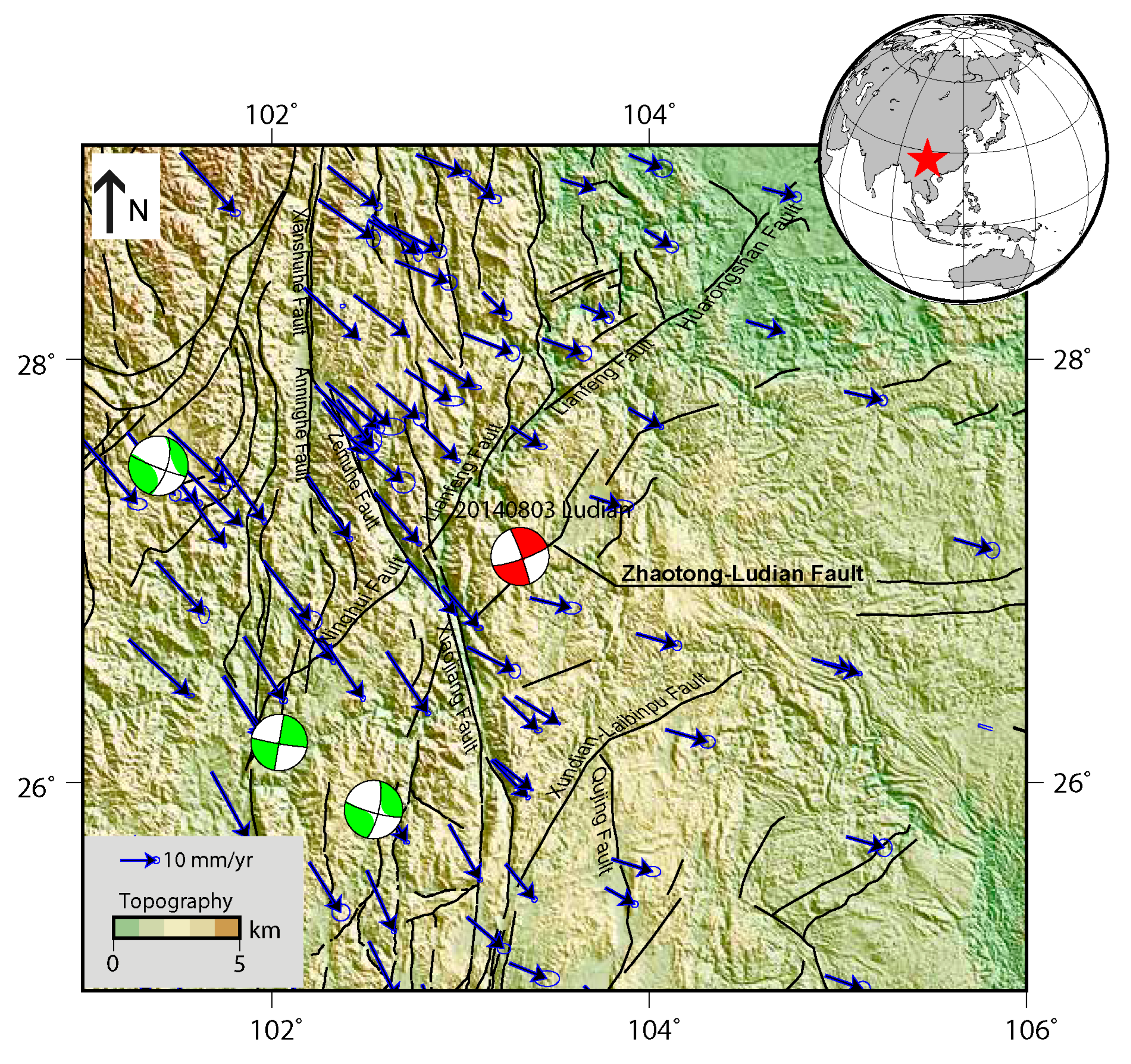
:1. Introduction
2. Observations
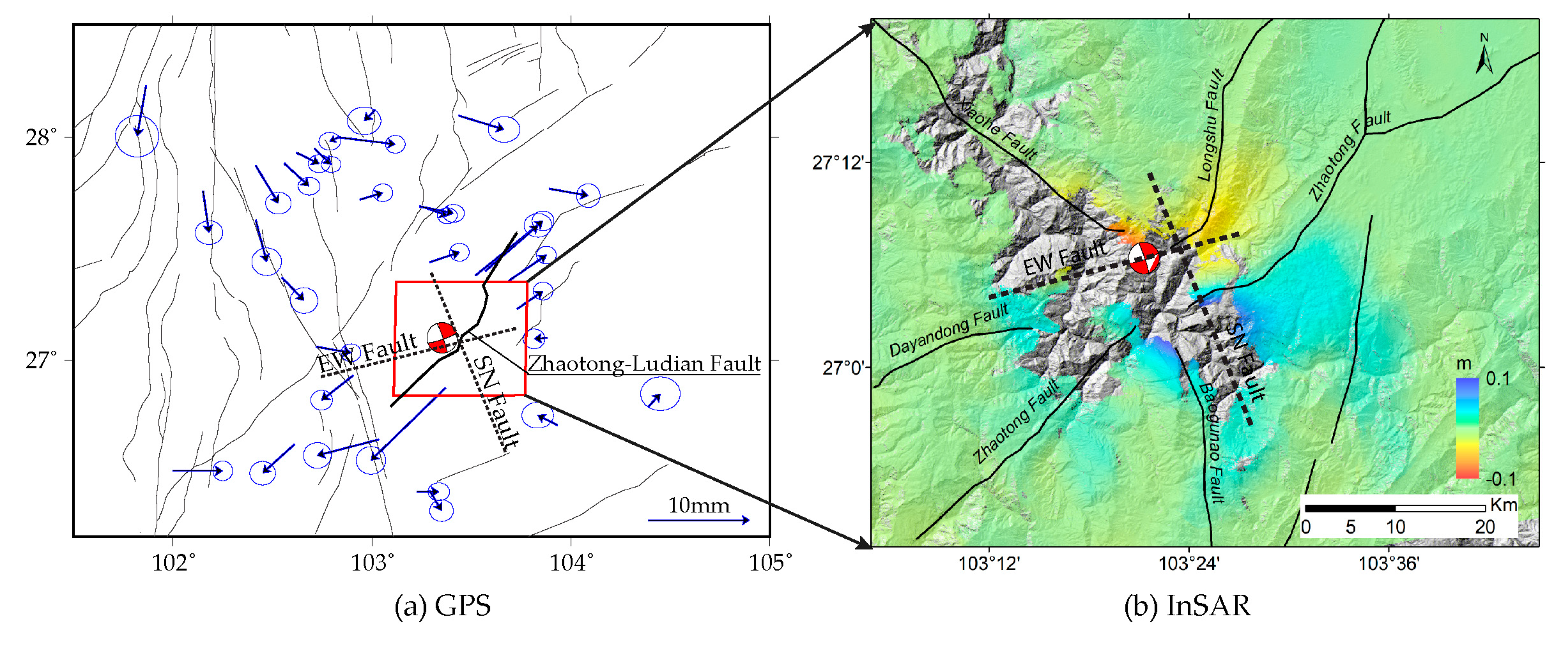
2.1. GPS Data and Analysis
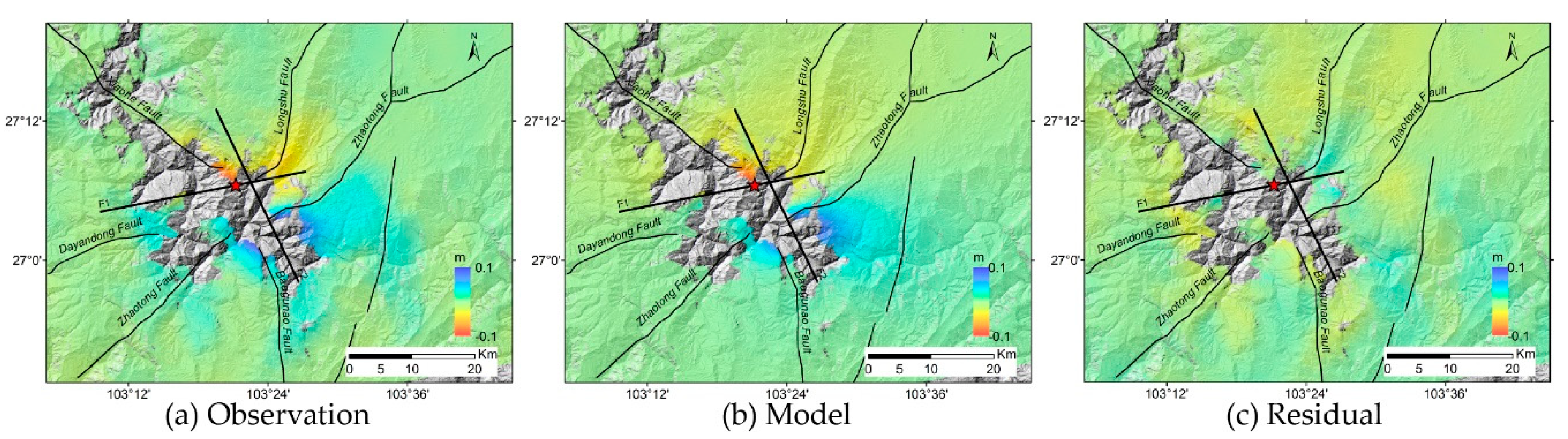
2.2. InSAR Data and Analysis
3. Coseismic Deformation Modeling
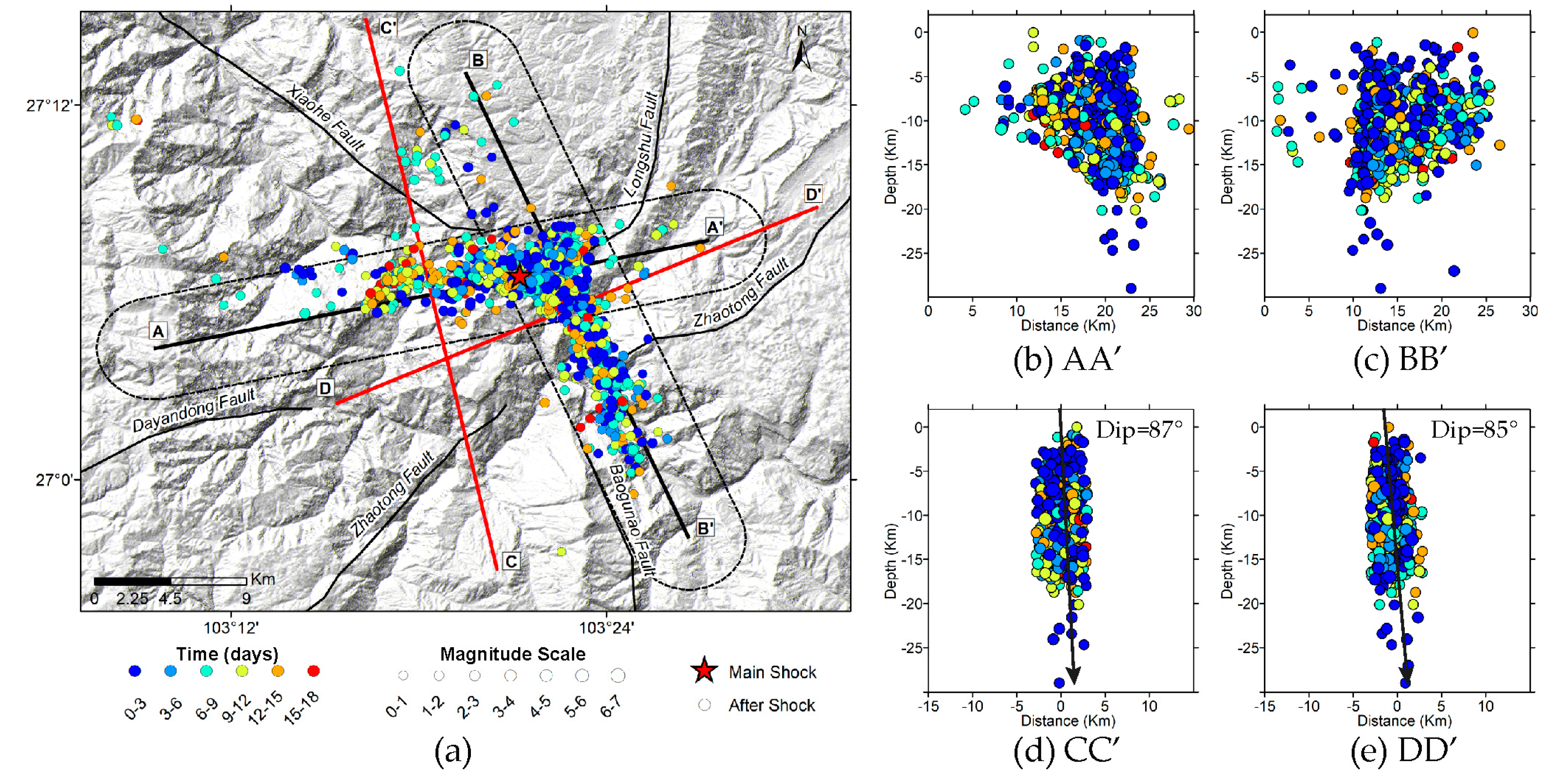
3.1. Fault Geometry
3.2. Coseismic Slip Distributions
4. Discussion
4.1. Comparison With Previous Studies
4.2. Coulomb Static Stress Change
5. Conclusions
Supplementary Materials
Author Contributions
Funding
Acknowledgments
Conflicts of Interest
References
- Xu, X.W.; Wen, X.; Zheng, R.; Ma, W.; Song, F.; Yu, G. Pattern of latest tectonic motion and its dynamics for active blocks in Sichuan-Yunnan region, China. Sci. China Ser. D Earth Sci. 2003, 46, 210–226. [Google Scholar]
- Wen, X.Z.; Du, F.; Yi, G.X.; Long, F.; Fan, J.; Yang, P.X.; Xiong, R.W.; Liu, X.X.; Liu, Q. Earthquake potential of the Zhaotong and Lianfeng fault zones of the eastern Sichuan-Yunnan border region. Chin. J. Geophys. 2013, 56, 3361–3372. [Google Scholar]
- Kan, R.J.; Zhang, S.C.; Yan, L.S.; Yu, F.T. Present Tectonic Stress Field and Its Relation to the Characteristics of Recent Tectonic Activity in Southwestern China. Chin. J. Sin. 1977, 2, 96–109. [Google Scholar]
- Kan, R.; Wang, S.; Huang, K.; Sung, W. Modern tectonic stress field and relative motion of intraplate block in Southwestern China. Seismol. Geol. 1983, 5, 79–90. [Google Scholar]
- Xu, L.S.; Zhang, X.; Yan, C.; Li, C.L. Analysis of the Love waves for the source complexity of the Ludian M (s) 6.5 earthquake. Chin. J. Geophys. 2014, 57, 3006–3017. [Google Scholar]
- Zhang, Y.; Xu, L.S.; Chen, Y.T.; Liu, R.F. Rupture process of the 3 August 2014 Ludian, Yunnan, M (w) 6.1 (M (s) 6.5) earthquake. Chin. J. Geophys. 2014, 57, 3052–3059. [Google Scholar]
- Liu, C.; Xu, L.S.; Chen, Y.T. The 3 August 2014, Ms 6.5 Ludian Earthquake. Available online: http://www.cea-igp.ac.cn/tpxw/270724.html (accessed on 1 November 2018).
- Fang, L.H.; Wu, J.P.; Wang, W.L.; Lü, Z.; Wang, C.; Yang, T.; Zhong, S. Relocation of the aftershock sequence of the Ms 6.5 Ludian earthquake and its seismogenic structure. Seismol. Geol. 2014, 36, 1173–1185. [Google Scholar]
- Zhang, G.W.; Lei, J.S.; Liang, S.S.; Sun, C.Q. Relocations and focal mechanism solutions of the 3 August 2014 Ludian, Yunnan M (s) 6.5 earthquake sequence. Chin. J. Geophys. 2014, 57, 3018–3027. [Google Scholar]
- Wang, W.L.; Wu, J.P.; Fang, L.H.; Lai, G.J. Double difference location of the Ludian M (s) 6.5 earthquake sequences in Yunnan province in 2014. Chin. J. Geophys. 2014, 57, 3042–3051. [Google Scholar]
- Xu, X.W.; Jiang, G.Y.; Yu, G.H.; Wu, X.Y.; Zhang, J.G.; Li, X. Discussion on seismogenic fault of the Ludian M (s) 6.5 earthquake and its tectonic attribution. Chin. J. Geophys. 2014, 57, 3060–3068. [Google Scholar]
- Cheng, J.; Wu, Z.; Liu, J.; Jiang, C.; Xu, X.; Fang, L.; Zhao, X.; Feng, W.; Liu, R.; Liang, J. Preliminary report on the 3 August 2014, M w 6.2/M s 6.5 Ludian, Yunnan–Sichuan border, southwest China, earthquake. Seismol. Res. Lett. 2015, 86, 750–763. [Google Scholar] [CrossRef]
- Zhang, Y.; Chen, Y.T.; Xu, L.S.; Wei, X.; Jin, M.P.; Zhang, S. The 2014 M (w) 6.1 Ludian, Yunnan, earthquake: A complex conjugated ruptured earthquake. Chin. J. Geophys. 2015, 58, 153–162. [Google Scholar]
- Guo, Z. Moment Tensor Solution of Ms6.5 2014 Ludian Earthquake. Available online: http://www.eq-igl.ac.cn/upload/files/2014/10/21112032347.pdf (accessed on 20 October 2018).
- Wang, R.; Diao, F.; Hoechner, A. SDM-A Geodetic Inversion Code Incorporating with Layered Crust Structure and Curved Fault Geometry. In Proceedings of the EGU General Assembly Conference Abstracts, Vienna, Austria, 7–12 April 2013. [Google Scholar]
- Zheng, G.; Wang, H.; Wright, T.J.; Lou, Y.; Zhang, R.; Zhang, W.; Shi, C.; Huang, J.; Wei, N. Crustal deformation in the India-Eurasia collision zone from 25 years of GPS measurements. J. Geophys. Res. Solid Earth 2017, 122, 9290–9312. [Google Scholar] [CrossRef]
- Wei, W.X.; Jiang, Z.S.; Shao, D.S.; Shao, Z.G.; Liu, X.X.; Zou, Z.Y.; Wang, Y. Coseismic displacements from GPS and inversion analysis for the 2014 Ludian 6. 5 earthquake. Chin. J. Geophys. 2018, 61, 1258–1265. [Google Scholar]
- Morena, L.; James, K.; Beck, J. An introduction to the RADARSAT-2 mission. Can. J. Remote Sens. 2004, 30, 221–234. [Google Scholar] [CrossRef]
- Thompson, A.A.; Luscombe, A.; James, K.; Fox, P. Radarsat-2 Mission Status: Capabilities Demonstrated and Image Quality Achieved. In Proceedings of the 7th European Conference on Synthetic Aperture Radar, Friedrichshafen, Germany, 2–5 June 2008; pp. 1–4. [Google Scholar]
- Rosen, P.A.; Hensley, S.; Joughin, I.R.; Li, F.K.; Madsen, S.N.; Rodriguez, E.; Goldstein, R.M. Synthetic aperture radar interferometry. Proc. IEEE 2000, 88, 333–382. [Google Scholar] [CrossRef]
- Massonnet, D.; Rossi, M.; Carmona, C.; Adragna, F.; Peltzer, G.; Feigl, K.; Rabaute, T. The displacement field of the Landers earthquake mapped by radar interferometry. Nature 1993, 364, 138. [Google Scholar] [CrossRef]
- Lu, Z.; Dzurisin, D. Ground surface deformation patterns, magma supply, and magma storage at Okmok volcano, Alaska, from InSAR analysis: 2. Coeruptive deflation, July–August 2008. J. Geophys. Res. Solid Earth 2010, 115. [Google Scholar] [CrossRef] [Green Version]
- Ji, L.; Wang, Q.; Xu, J.; Ji, C. The July 11, 1995 Myanmar–China earthquake: A representative event in the bookshelf faulting system of southeastern Asia observed from JERS-1 SAR images. Int. J. Appl. Earth Obs. Geoinf. 2017, 55, 43–51. [Google Scholar] [CrossRef]
- Lu, Z.; Dzurisin, D. InSAR imaging of Aleutian volcanoes. In InSAR Imaging of Aleutian Volcanoes; Springer: Chichester, UK, 2014; pp. 87–345. Available online: https://0-link-springer-com.brum.beds.ac.uk/chapter/10.1007/978-3-642-00348-6_6 (accessed on 15 October 2019).
- Rosen, P.A.; Hensley, S.; Zebker, H.A.; Webb, F.H.; Fielding, E.J. Surface deformation and coherence measurements of Kilauea Volcano, Hawaii, from SIR-C radar interferometry. J. Geophys. Res. Planets 1996, 101, 23109–23125. [Google Scholar] [CrossRef]
- Chen, X.; Hu, K.; Ge, Y.; Wang, Y. Surface ruptures and large-scale landslides caused by “8· 03” Ludian Earthquake in Yunnan, China. Mt. Res. 2015, 1, 65–71. [Google Scholar]
- Chen, X.L.; Liu, C.G.; Wang, M.M.; Zhou, Q. Causes of unusual distribution of coseismic landslides triggered by the Mw 6.1 2014 Ludian, Yunnan, China earthquake. J. Asian Earth Sci. 2018, 159, 17–23. [Google Scholar] [CrossRef]
- Shi, Z.; Xiong, X.; Peng, M.; Zhang, L.; Xiong, Y.; Chen, H.; Zhu, Y. Risk assessment and mitigation for the Hongshiyan landslide dam triggered by the 2014 Ludian earthquake in Yunnan, China. Landslides 2017, 14, 269–285. [Google Scholar] [CrossRef]
- Xu, C. Utilizing coseismic landslides to analyze the source and rupturing process of the 2014 Ludian earthquake. J. Eng. Geol. 2015, 23, 755–759. [Google Scholar]
- Xu, C.; Xu, X.W.; Shen, L.L.; Du, S.; Wu, S.; Tian, Y.; Li, X. Inventory of landslides triggered by the 2014 Ms 6.5 Ludian earthquake and its implications on several earthquake parameters. Seism. Geol. 2014, 36, 1186–1203. [Google Scholar]
- Zhou, S.; Chen, G.; Fang, L. Distribution pattern of landslides triggered by the 2014 Ludian earthquake of China: Implications for regional threshold topography and the seismogenic fault identification. ISPRS Int. J. Geo Inf. 2016, 5, 46. [Google Scholar] [CrossRef] [Green Version]
- Lin, X.; Zhang, H.; Chen, H.; Chen, H.; Lin, J. Field investigation on severely damaged aseismic buildings in 2014 Ludian earthquake. Earthq. Eng. Eng. Vib. 2015, 14, 169–176. [Google Scholar] [CrossRef]
- Laske, G.; Masters, G.; Ma, Z.; Pasyanos, M. Update on CRUST1. 0—A 1-Degree Global Model of Earth’s Crust. Geophys. Res. Abstr. 2013, 15, 2658. [Google Scholar]
- Jónsson, S.; Zebker, H.; Segall, P.; Amelung, F. Fault slip distribution of the 1999 M w 7.1 Hector Mine, California, earthquake, estimated from satellite radar and GPS measurements. Bull. Seismol. Soc. Am. 2002, 92, 1377–1389. [Google Scholar]
- Ji, L.; Wang, Q.; Xu, J.; Feng, J. The 1996 Mw 6.6 Lijiang earthquake: Application of JERS-1 SAR interferometry on a typical normal-faulting event in the northwestern Yunnan rift zone, SW China. J. Asian Earth Sci. 2017, 146, 221–232. [Google Scholar] [CrossRef]
- Liu, C.L.; Zheng, Y.; Xiong, X.; Fu, R.; Shan, B.; Diao, F.Q. Rupture process of M (s) 6.5 Ludian earthquake constrained by regional broadband seismograms. Chin. J. Geophys. 2014, 57, 3028–3037. [Google Scholar]
- Heidbach, O.; Rajabi, M.; Cui, X.; Fuchs, K.; Müller, B.; Reinecker, J.; Reiter, K.; Tingay, M.; Wenzel, F.; Xie, F. The World Stress Map database release 2016: Crustal stress pattern across scales. Tectonophysics 2018, 744, 484–498. [Google Scholar] [CrossRef]
- Nissen, E.; Elliott, J.; Sloan, R.; Craig, T.; Funning, G.; Hutko, A.; Parsons, B.; Wright, T. Limitations of rupture forecasting exposed by instantaneously triggered earthquake doublet. Nat. Geosci. 2016, 9, 330. [Google Scholar] [CrossRef]


| No. | Solution | Magnitude | Longitude (°E) | Latitude (°N) | Depth (km) | Np1 (Strike, Dip, Rake) | Np2 (Strike, Dip, Rake) |
|---|---|---|---|---|---|---|---|
| 1 | IES 1 | 6.5 * | 103.3 | 27.1 | 12 | 341°/82°/−4° | 72°/86°/−172° |
| 2 | USGS 2 | 6.2 ** | 103.409 | 27.189 | 12 | 338°/74°/−32° | 77°/59°/−162° |
| 3 | GCMT 3 | 6.2 ** | 103.5 | 27.06 | 14.4 | 340°/86°/−9° | 71°/81°/−175° |
| 4 | Wang et al. [8,9,10,11,12,13] | 6.5 * | 103.354 | 27.109 | 15 | - | - |
| 5 | Liu et al. [7] | 6.2 ** | - | - | 11 | 167°/87°/6° | 74°/84°/177° |
| 6 | Guo et al. [14] | 6.1 ** | - | - | 14 | 160°/80°/−20° | 254°/70°/−189° |
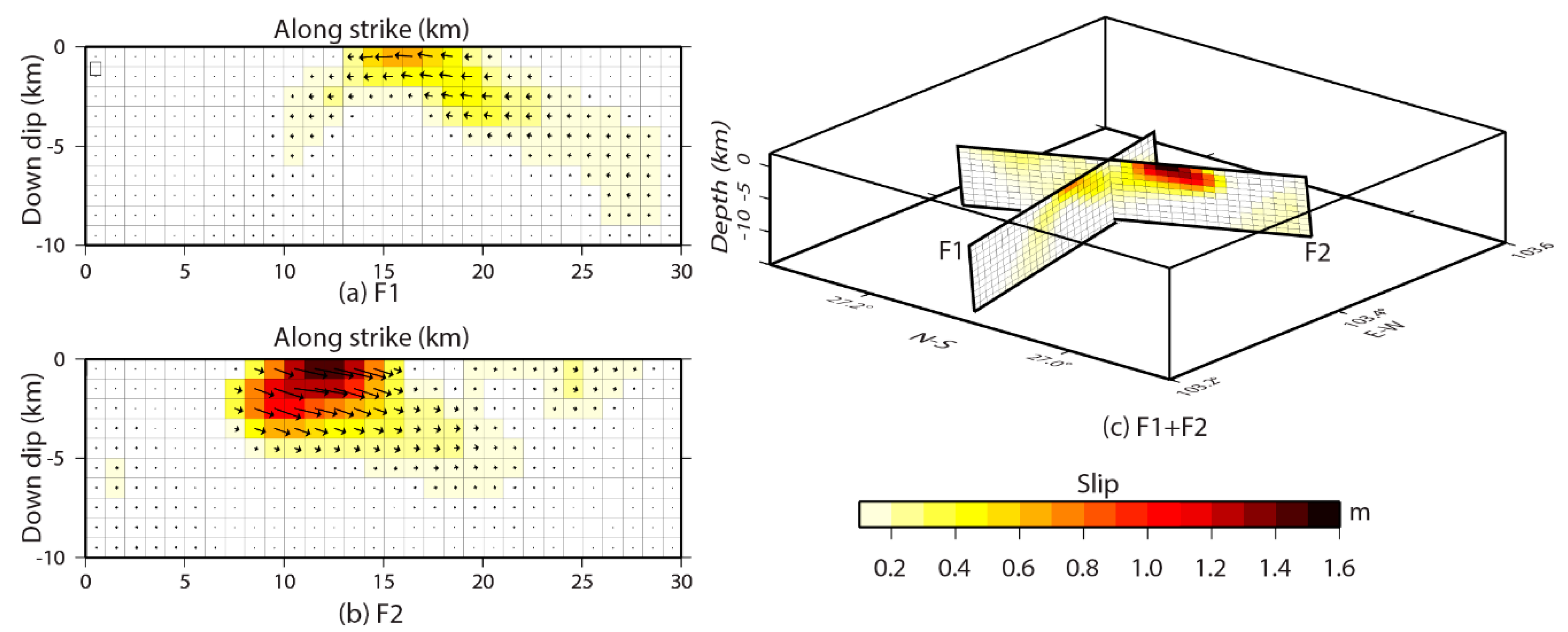
| No. | Direction | Strike (°) | Dip Angle (°) | Width (km) | Length (km) |
|---|---|---|---|---|---|
| F1 | NNW–SSE (AA’) | 337 | 87 | 30 | 30 |
| F2 | ENE–WSW (BB’) | 81 | 85 | 30 | 30 |
© 2019 by the authors. Licensee MDPI, Basel, Switzerland. This article is an open access article distributed under the terms and conditions of the Creative Commons Attribution (CC BY) license (http://creativecommons.org/licenses/by/4.0/).
Share and Cite
Niu, Y.; Wang, S.; Zhu, W.; Zhang, Q.; Lu, Z.; Zhao, C.; Qu, W. The 2014 Mw 6.1 Ludian Earthquake: The Application of RADARSAT-2 SAR Interferometry and GPS for this Conjugated Ruptured Event. Remote Sens. 2020, 12, 99. https://0-doi-org.brum.beds.ac.uk/10.3390/rs12010099
Niu Y, Wang S, Zhu W, Zhang Q, Lu Z, Zhao C, Qu W. The 2014 Mw 6.1 Ludian Earthquake: The Application of RADARSAT-2 SAR Interferometry and GPS for this Conjugated Ruptured Event. Remote Sensing. 2020; 12(1):99. https://0-doi-org.brum.beds.ac.uk/10.3390/rs12010099
Chicago/Turabian StyleNiu, Yufen, Shuai Wang, Wu Zhu, Qin Zhang, Zhong Lu, Chaoying Zhao, and Wei Qu. 2020. "The 2014 Mw 6.1 Ludian Earthquake: The Application of RADARSAT-2 SAR Interferometry and GPS for this Conjugated Ruptured Event" Remote Sensing 12, no. 1: 99. https://0-doi-org.brum.beds.ac.uk/10.3390/rs12010099