Tropical Cyclone Intensity Estimation Using Multi-Dimensional Convolutional Neural Networks from Geostationary Satellite Data


Abstract
:
1. Introduction
2. Data
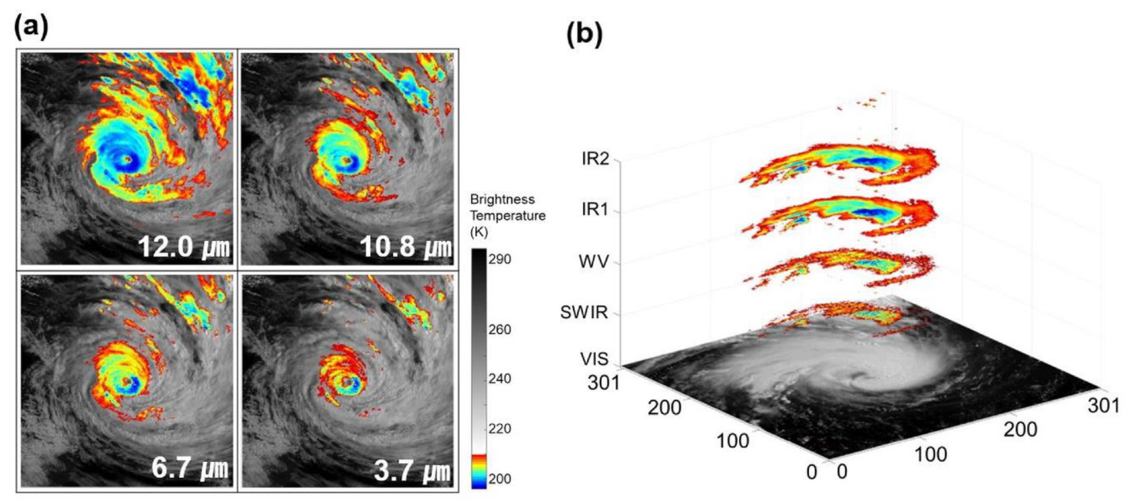
2.1. Geostationary Meteorological Satellite Sensor Data
2.2. Best Track Data
3. Methodology
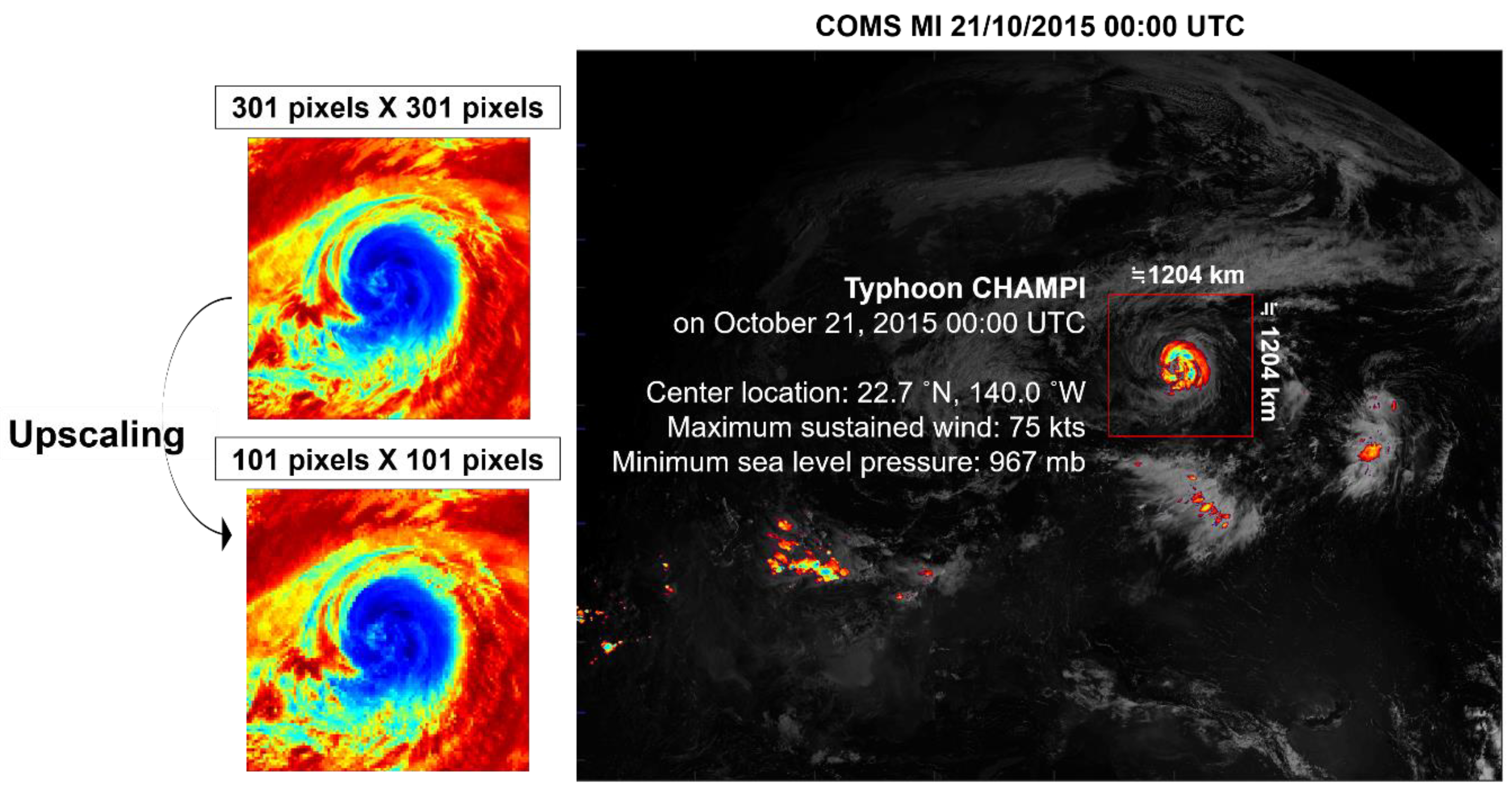
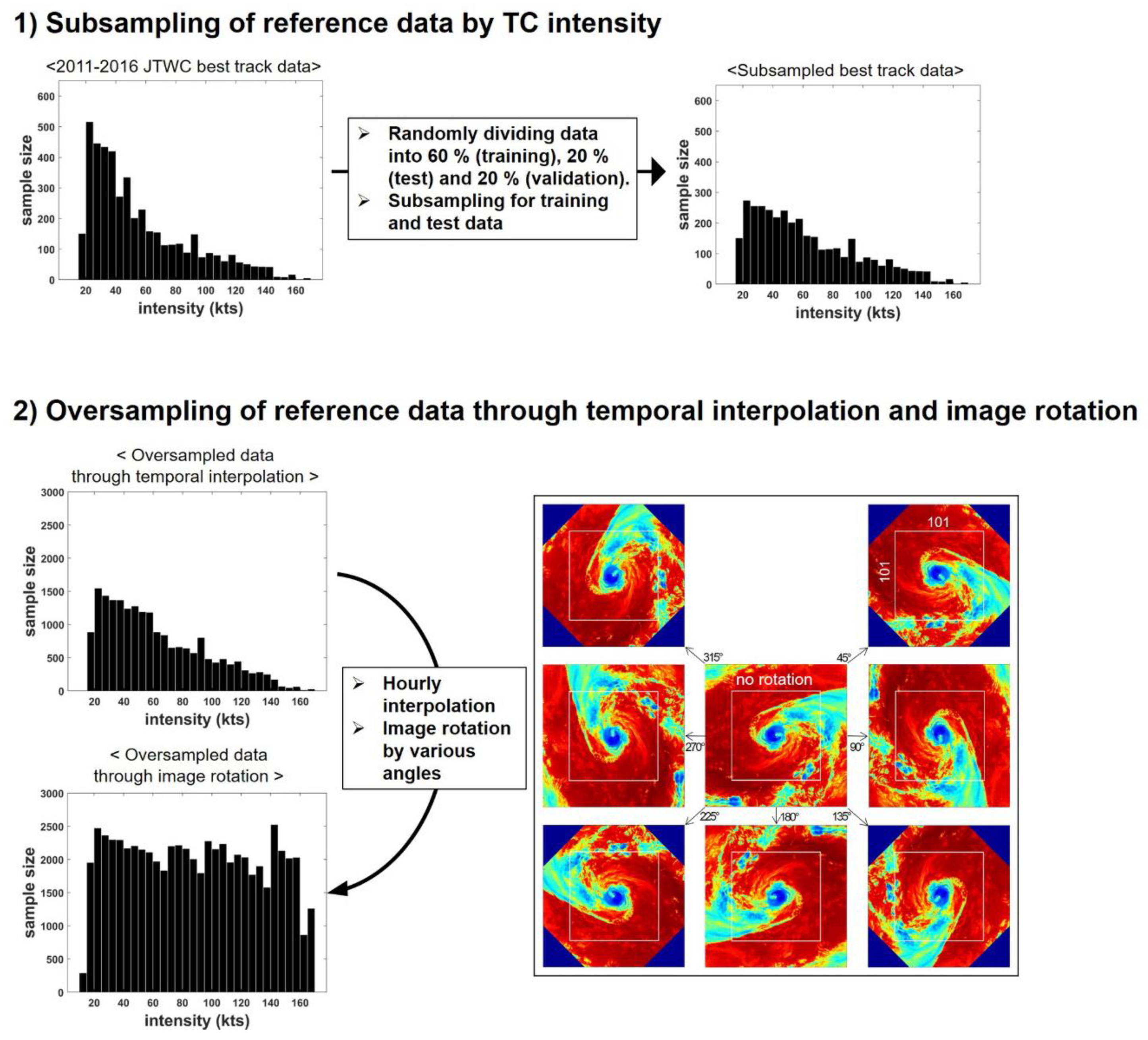
3.1. Input Data Preparation
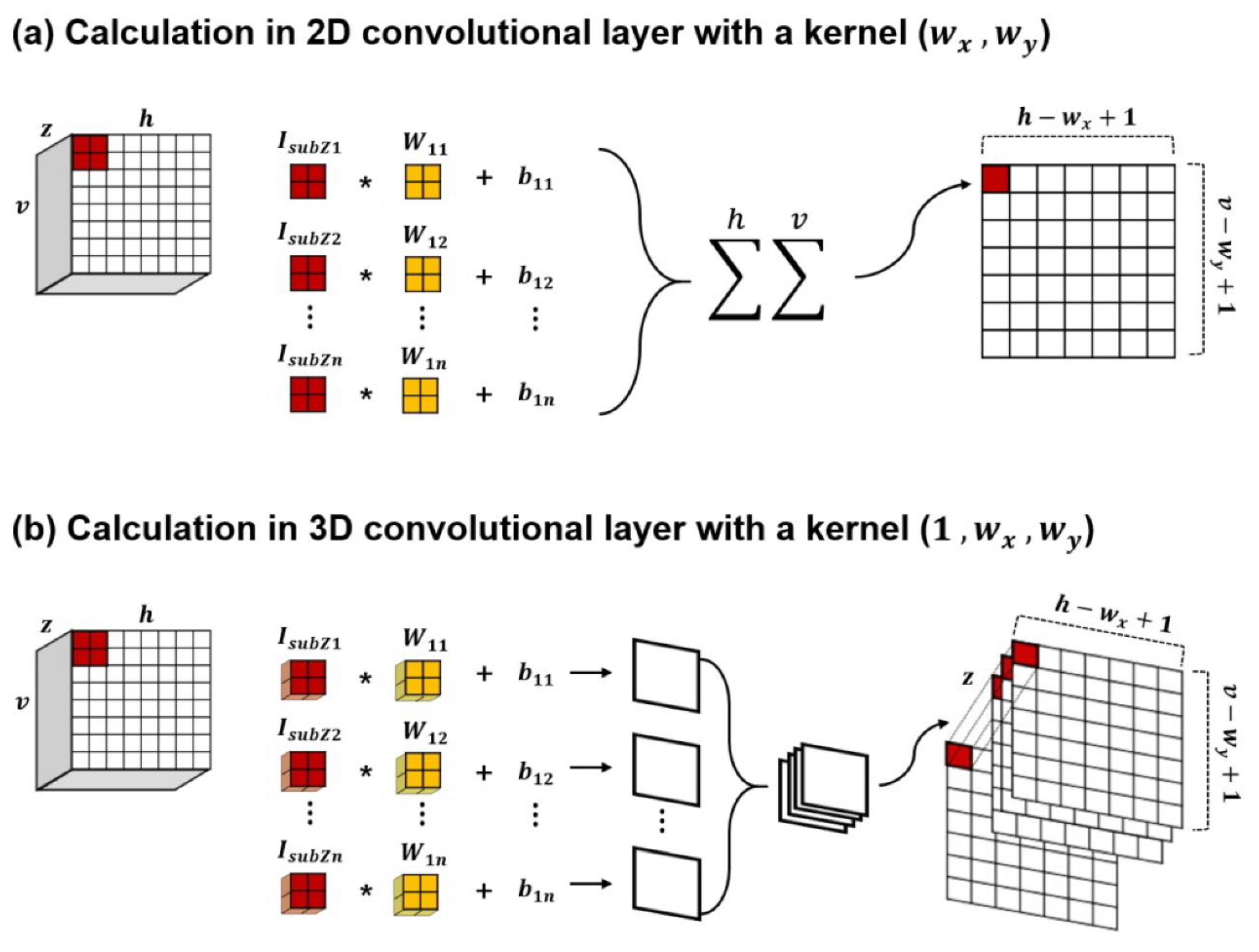
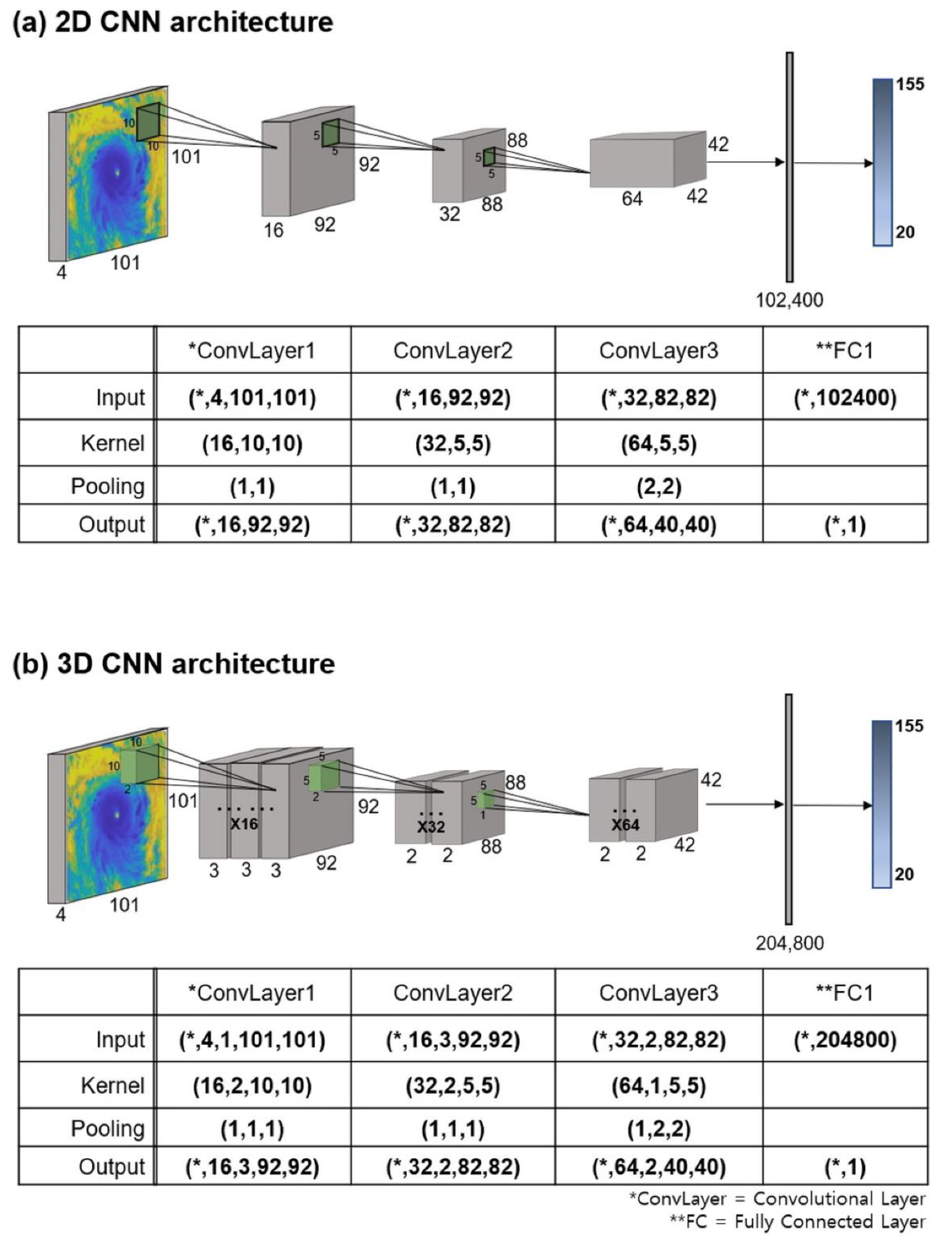
3.2. Convolutional Neural Networks (CNNs)
3.3. Optimization and Schemes
3.4. Accuracy Assessment
4. Results
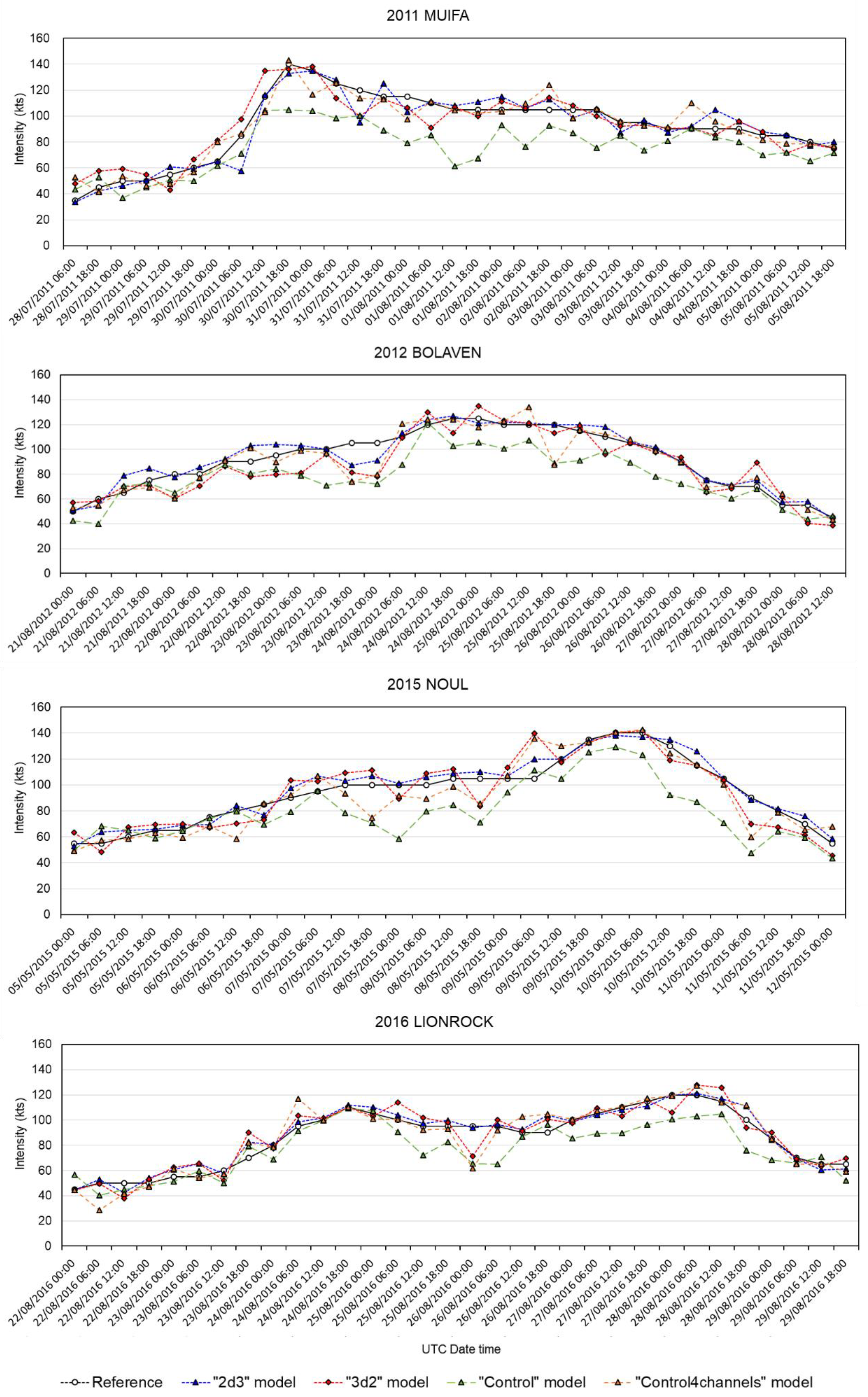
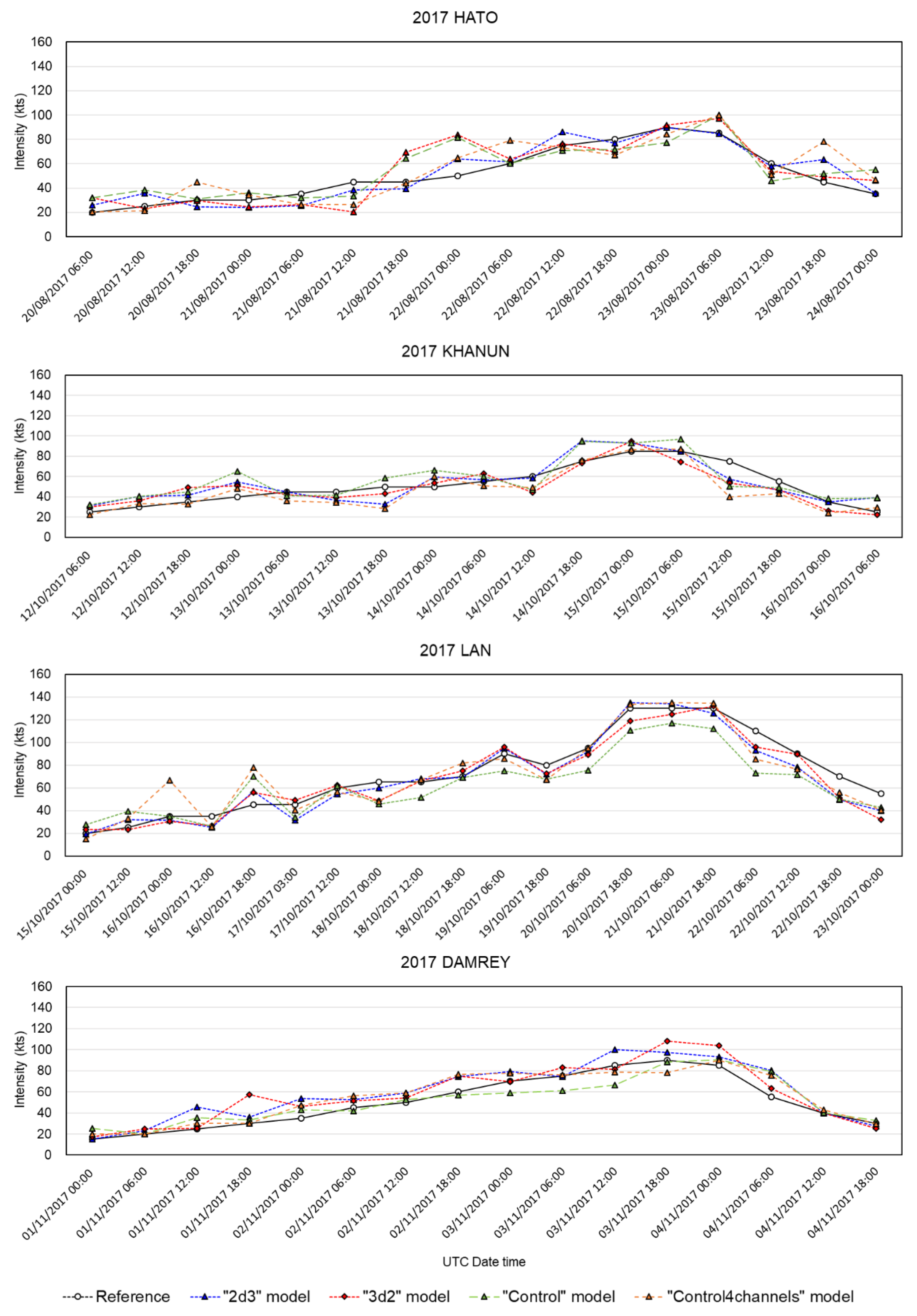
4.1. Modeling Performance
5. Discussion
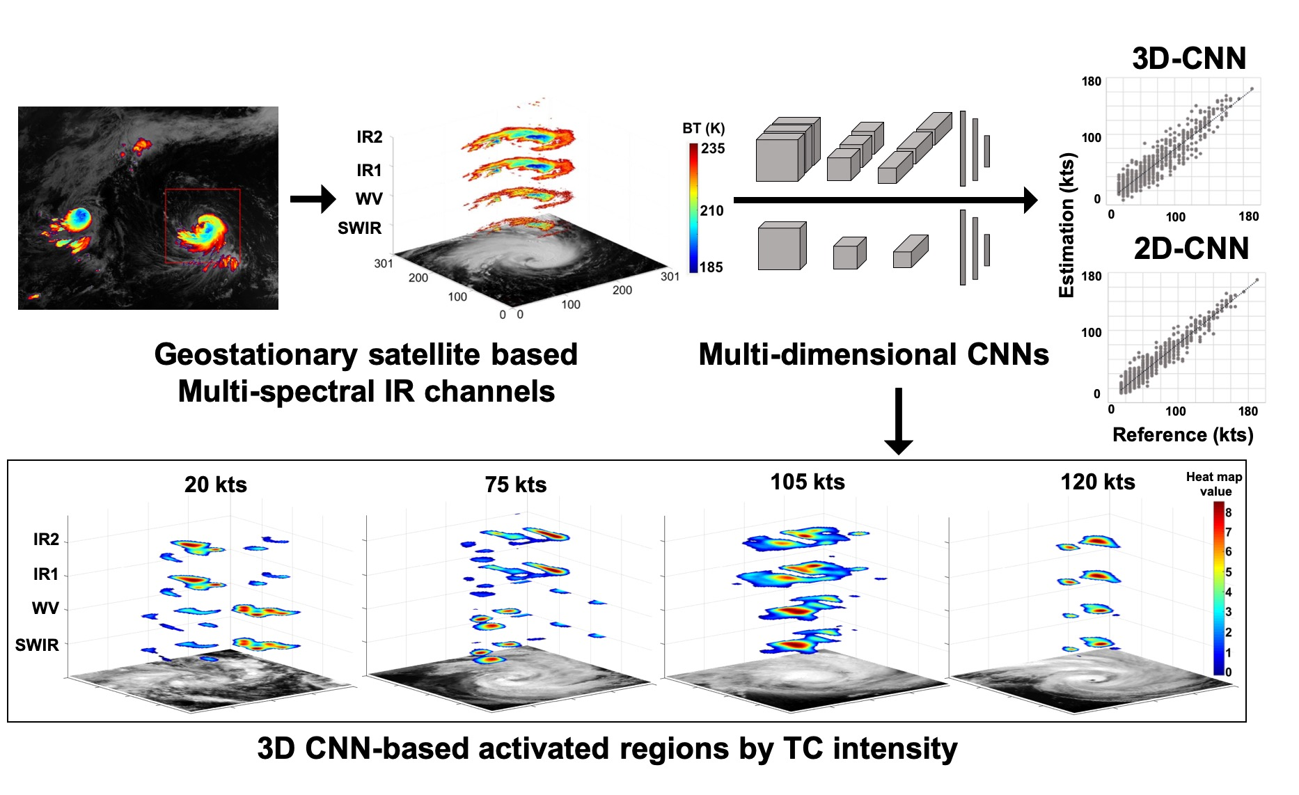
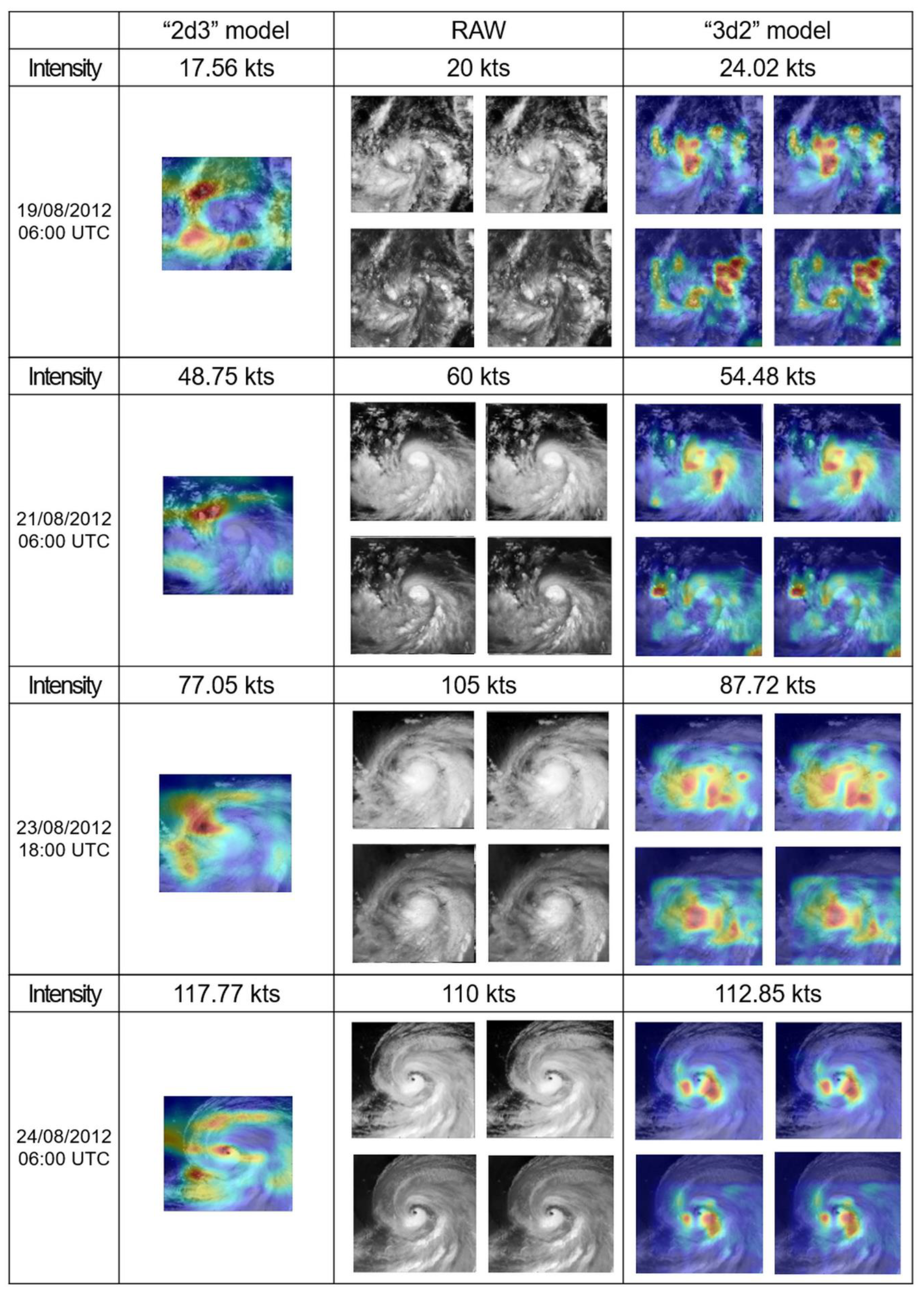
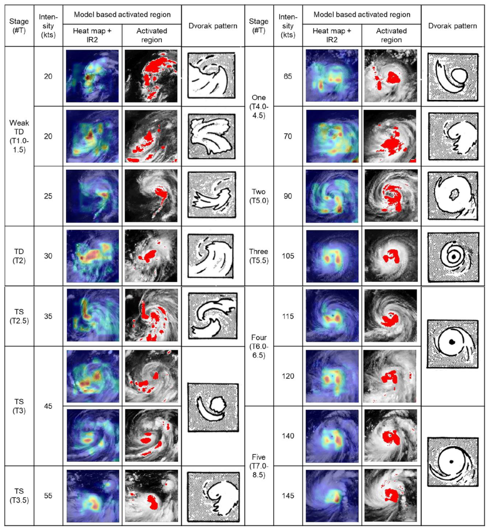
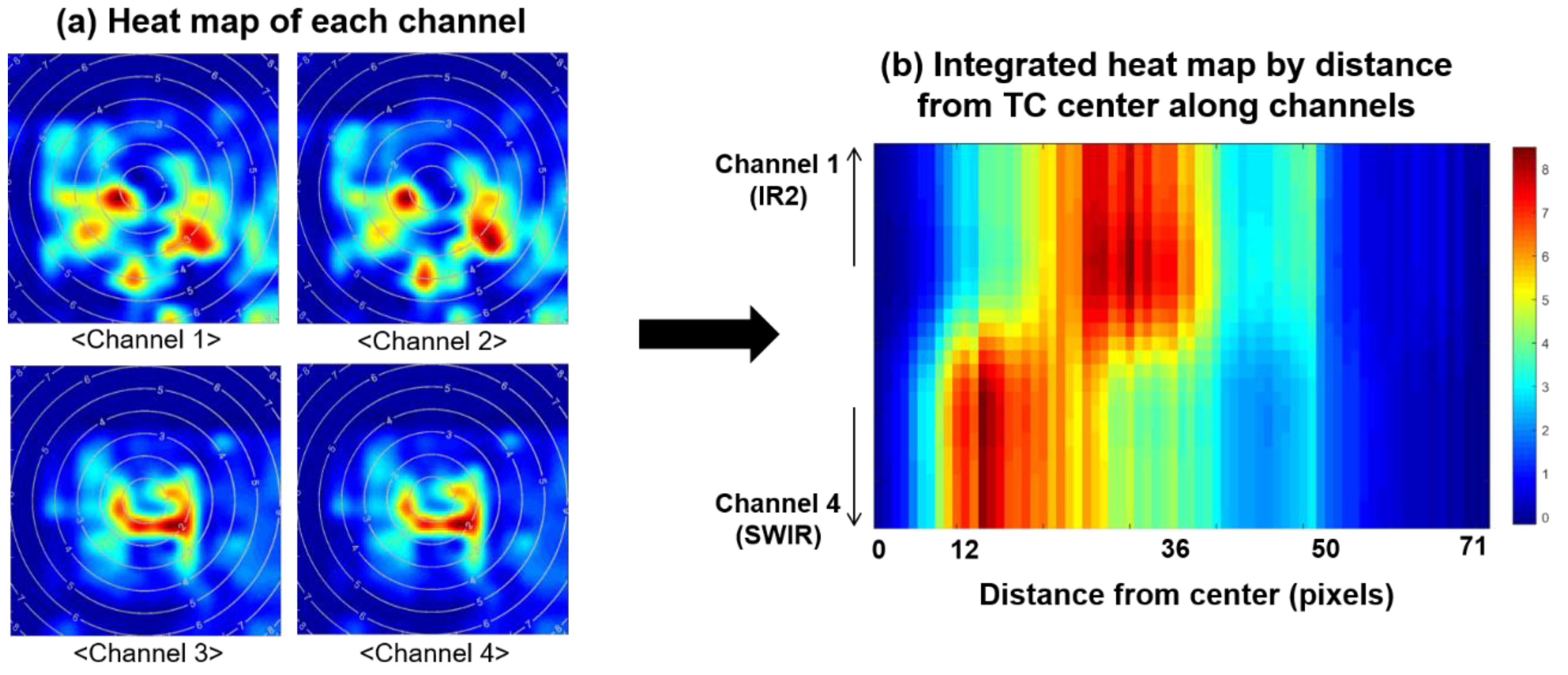
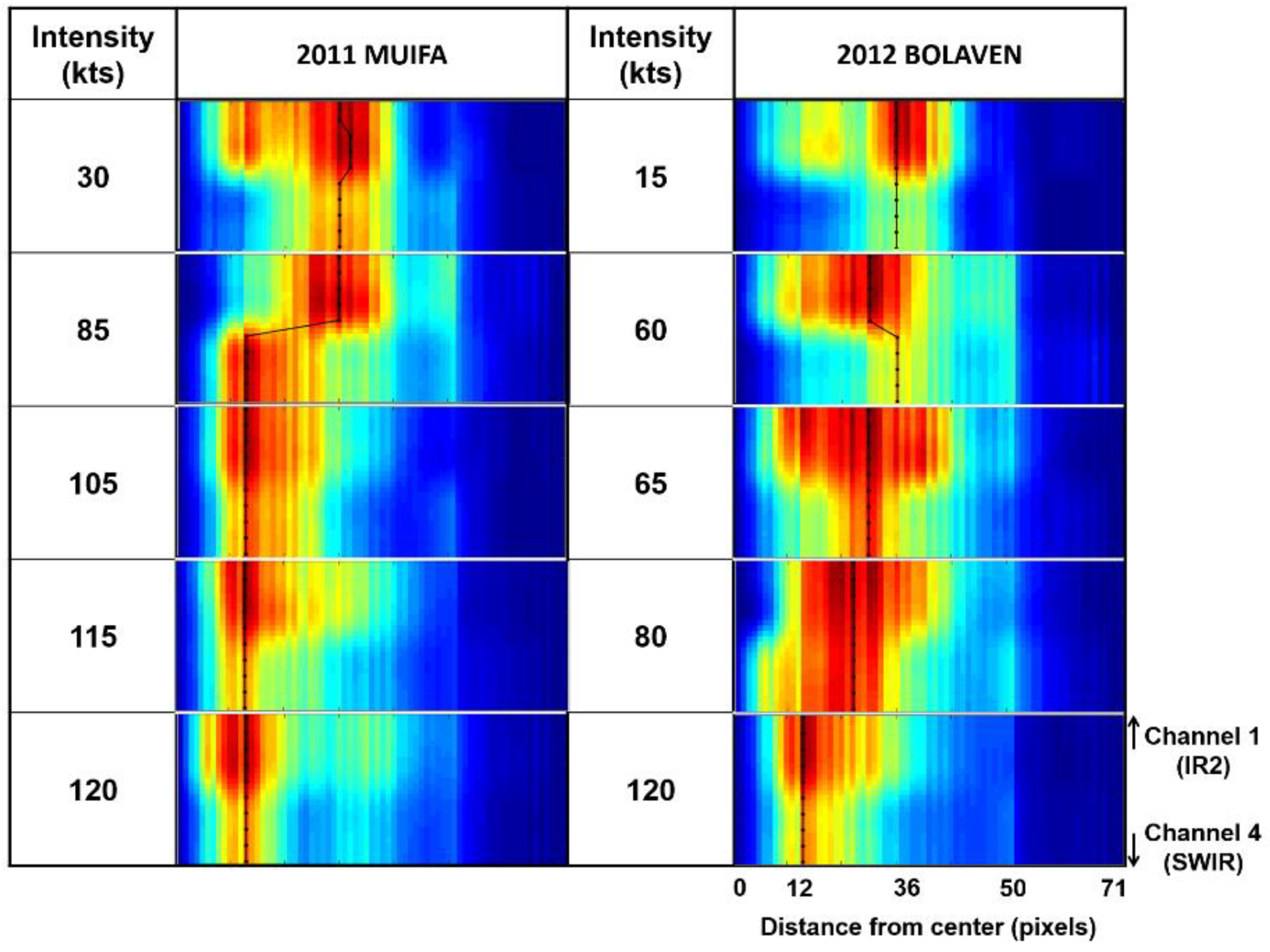
5.1. Visualization
5.2. Interpretation of Relationship between Multi-Spectral TC Images and Intensity
5.3. Novelty and Limitation
6. Conclusions
Author Contributions
Funding
Conflicts of Interest
References
- Seneviratne, S.I.; Nicholls, N.; Easterling, D.; Goodess, C.M.; Kanae, S.; Kossin, J.; Luo, Y.; Marengo, J.; McInnes, K.; Rahimi, M.; et al. Changes in climate extremes and their impacts on the natural physical environment. In Managing the Risks of Extreme Events and Disasters to Advance Climate Change Adaptation: Special Report of the Intergovernmental Panel on Climate Change; Cambridge University Press: Cambridge, UK, 2012; pp. 109–230. [Google Scholar]
- Hoegh-Guldberg, O.; Jacob, D.; Taylor, M. Impacts of 1.5 C Global Warming on Natural and Human Systems. In Global Warming of 1.5 C: An. IPCC Special Report on the Impacts of Global Warming of 1.5 C above Pre-Industrial Levels and Related Global Greenhouse Gas Emission Pathways, in the Context of Strengthening the Global Response to the Threat of Climate Change, Sustainable Development, and Efforts to Eradicate Poverty; MassonDelmotte, V., Zhai, P., Pörtner, H.O., Roberts, D., Skea, J., Shukla, P.R., Pirani, A., Moufouma-Okia, W., Péan, C., Pidcock, R., et al., Eds.; 2018; pp. 175–311, in press. [Google Scholar]
- Knutson, T.R.; McBride, J.L.; Chan, J.; Emanuel, K.; Holland, G.; Landsea, C.; Held, I.; Kossin, J.P.; Srivastava, A.K.; Sugi, M. Tropical cyclones and climate change. Nat. Geosci. 2010, 3, 157–163. [Google Scholar] [CrossRef] [Green Version]
- World Bank. Information, Communication Technologies, and infoDev (Program). In Information and Communications for Development 2012: Maximizing Mobile; World Bank Publications: Washington, DC, USA, 2012. [Google Scholar]
- Mendelsohn, R.; Emanuel, K.; Chonabayashi, S.; Bakkensen, L. The impact of climate change on global tropical cyclone damage. Nat. Clim. Chang. 2012, 2, 205–209. [Google Scholar] [CrossRef]
- Schmetz, J.; Tjemkes, S.A.; Gube, M.; Van de Berg, L. Monitoring deep convection and convective overshooting with METEOSAT. Adv. Space Res. 1997, 19, 433–441. [Google Scholar] [CrossRef]
- Dvorak, V.F. Tropical cyclone intensity analysis using satellite data. In NOAA Technical Report NESDIS, 11; US Department of Commerce, National Oceanic and Atmospheric Administration, National Environmental Satellite, Data, and Information Service: Washington, DC, USA, 1984; pp. 1–47. [Google Scholar]
- Menzel, W.P.; Purdom, J.F. Introducing GOES-I: The First of a New Generation of Geostationary Operational Environmental Satellites. Bull. Am. Meteorol. Soc. 1994, 75, 757–781. [Google Scholar] [CrossRef] [Green Version]
- Dvorak, V.F. Tropical Cyclone Intensity Analysis and Forecasting from Satellite Imagery. Mon. Weather Rev. 1975, 103, 420–430. [Google Scholar] [CrossRef]
- Olander, T.L.; Velden, C.S. The advanced Dvorak technique: Continued development of an objective scheme to estimate tropical cyclone intensity using geostationary infrared satellite imagery. Weather Forecast. 2007, 22, 287–298. [Google Scholar] [CrossRef]
- Olander, T.L.; Velden, C.S. The Advanced Dvorak Technique (ADT) for Estimating Tropical Cyclone Intensity: Update and New Capabilities. Weather Forecast. 2019, 34, 905–922. [Google Scholar] [CrossRef]
- Velden, C.S.; Olander, T.L.; Zehr, R.M. Development of an Objective Scheme to Estimate Tropical Cyclone Intensity from Digital Geostationary Satellite Infrared Imagery. Weather Forecast. 1998, 13, 172–186. [Google Scholar] [CrossRef] [Green Version]
- Velden, C.; Harper, B.; Wells, F.; Beven, J.L.; Zehr, R.; Olander, T.; Mayfield, M.; Guard, C.C.; Lander, M.; Edson, R.; et al. The Dvorak Tropical Cyclone Intensity Estimation Technique: A Satellite-Based Method that Has Endured for over 30 Years. Bull. Am. Meteorol. Soc. 2006, 87, 1195–1210. [Google Scholar] [CrossRef]
- Velden, C.S.; Hayden, C.M.; Nieman, S.J.W.; Paul Menzel, W.; Wanzong, S.; Goerss, J.S. Upper-tropospheric winds derived from geostationary satellite water vapor observations. Bull. Am. Meteorol. Soc. 1997, 78, 173–195. [Google Scholar] [CrossRef] [Green Version]
- Piñeros, M.F.; Ritchie, E.A.; Tyo, J.S. Objective measures of tropical cyclone structure and intensity change from remotely sensed infrared image data. IEEE Trans. Geosci. Remote Sens. 2008, 46, 3574–3580. [Google Scholar] [CrossRef]
- Ritchie, E.A.; Wood, K.M.; Rodríguez-Herrera, O.G.; Piñeros, M.F.; Tyo, J.S. Satellite-derived tropical cyclone intensity in the north pacific ocean using the deviation-angle variance technique. Weather Forecast. 2014, 29, 505–516. [Google Scholar] [CrossRef] [Green Version]
- Pradhan, R.; Aygun, R.S.; Maskey, M.; Ramachandran, R.; Cecil, D.J. Tropical cyclone intensity estimation using a deep convolutional neural network. IEEE Trans. Image Process. 2018, 27, 692–702. [Google Scholar] [CrossRef] [PubMed]
- Combinido, J.S.; Mendoza, J.R.; Aborot, J. A Convolutional Neural Network Approach for Estimating Tropical Cyclone Intensity Using Satellite-based Infrared Images. In Proceedings of the 2018 24th ICPR, Beijing, China, 20–24 August 2018. [Google Scholar]
- Simonyan, K.; Zisserman, A. Very deep convolutional networks for large-scale image recognition. In Proceedings of the ICLR 2015, San Diego, CA, USA, 7–9 May 2015. [Google Scholar]
- Wimmers, A.; Velden, C.; Cossuth, J.H. Using deep learning to estimate tropical cyclone intensity from satellite passive microwave imagery. Mon. Weather Rev. 2019, 147, 2261–2282. [Google Scholar] [CrossRef]
- Elsberry, R.L.; Jeffries, R.A. Vertical wind shear influences on tropical cyclone formation and intensification during TCM-92 and TCM-93. Mon. Weather Rev. 1996, 124, 1374–1387. [Google Scholar] [CrossRef] [Green Version]
- LeCun, Y.; Boser, B.E.; Denker, J.S.; Henderson, D.; Howard, R.E.; Hubbard, W.E.; Jackel, L.D. Handwritten digit recognition with a back-propagation network. In Advances in Neural Information Processing Systems; MITpress: Cambridge, MA, US. 1990; pp. 396–404. [Google Scholar]
- Yang, H.; Yu, B.; Luo, J.; Chen, F. Semantic segmentation of high spatial resolution images with deep neural networks. GISci. Remote Sens. 2019, 56, 749–768. [Google Scholar] [CrossRef]
- Liu, T.; Abd-Elrahman, A.; Morton, J.; Wilhelm, V.L. Comparing fully convolutional networks, random forest, support vector machine, and patch-based deep convolutional neural networks for object-based wetland mapping using images from small unmanned aircraft system. GISci. Remote Sens. 2018, 55, 243–264. [Google Scholar] [CrossRef]
- Kim, M.; Lee, J.; Im, J. Deep learning-based monitoring of overshooting cloud tops from geostationary satellite data. GISci. Remote Sens. 2018, 55, 763–792. [Google Scholar] [CrossRef]
- Yu, X.; Wu, X.; Luo, C.; Ren, P. Deep learning in remote sensing scene classification: A data augmentation enhanced convolutional neural network framework. GISci. Remote Sens. 2017, 54, 741–758. [Google Scholar] [CrossRef] [Green Version]
- Ou, M.L.; Jae-Gwang-Won, S.R.C. Introduction to the COMS Program and its application to meteorological services of Korea. In Proceedings of the 2005 EUMETSAT Meteorological Satellite Conference, Dubrovnik, Croatia, 19 September 2005; pp. 19–23. [Google Scholar]
- Ralph, F.M.; Neiman, P.J.; Wick, G.A. Satellite and CALJET aircraft observations of atmospheric rivers over the eastern North Pacific Ocean during the winter of 1997/98. Mon. Weather Rev. 2004, 132, 1721–1745. [Google Scholar] [CrossRef] [Green Version]
- Durry, G.; Amarouche, N.; Zéninari, V.; Parvitte, B.; Lebarbu, T.; Ovarlez, J. In situ sensing of the middle atmosphere with balloonborne near-infrared laser diodes. Spectrochim. Acta Part A 2004, 60, 3371–3379. [Google Scholar] [CrossRef] [PubMed]
- Lee, T.F.; Turk, F.J.; Richardson, K. Stratus and fog products using GOES-8–9 3.9-μ m data. Weather Forecast. 1997, 12, 664–677. [Google Scholar] [CrossRef]
- Nakajima, T.; King, M.D. Determination of the Optical Thickness and Effective Particle Radius of Clouds from Reflected Solar Radiation Measurements. Part I: Theory. J. Atmos. Sci. 1990, 47, 1878–1893. [Google Scholar] [CrossRef] [Green Version]
- Rosenfeld, D.; Woodley, W.L.; Lerner, A.; Kelman, G.; Lindsey, D.T. Satellite detection of severe convective storms by their retrieved vertical profiles of cloud particle effective radius and thermodynamic phase. J. Geophys. Res. Atmos. 2008, 113, D04208. [Google Scholar] [CrossRef] [Green Version]
- Martins, J.V.; Marshak, A.; Remer, L.A.; Rosenfeld, D.; Kaufman, Y.J.; Fernandez-Borda, R.; Koren, I.; Correia, A.L.; Artaxo, P. Remote sensing the vertical profile of cloud droplet effective radius, thermodynamic phase, and temperature. Atmos. Chem. Phys. 2011, 11, 9485–9501. [Google Scholar] [CrossRef] [Green Version]
- Lowry, M.R. Developing a Unified Superset in Quantifying Ambiguities among Tropical Cyclone Best Track Data for the Western North Pacific. Master’s Thesis, Dept. Meteorology, Florida State University, Tallahassee, FL, USA, 2008. [Google Scholar]
- Guard, C.P.; Carr, L.E.; Wells, F.H.; Jeffries, R.A.; Gural, N.D.; Edson, D.K. Joint Typhoon Warning Center and the Challenges of Multibasin Tropical Cyclone Forecasting. Weather Forecast. 1992, 7, 328–352. [Google Scholar] [CrossRef] [Green Version]
- Knapp, K.R.; Kruk, M.C.; Levinson, D.H.; Diamond, H.J.; Neumann, C.J. The International Best Track Archive for Climate Stewardship (IBTrACS). Bull. Am. Meteorol. Soc. 2010, 91, 363–376. [Google Scholar] [CrossRef]
- Longadge, R.; Dongre, S. Class Imbalance Problem in Data Mining Review. arXiv 2013, arXiv:1305.1707. [Google Scholar]
- Romero, A.; Gatta, C.; Camps-Valls, G. Unsupervised deep feature extraction for remote sensing image classification. IEEE Trans. Image Process. 2015, 54, 1349–1362. [Google Scholar] [CrossRef] [Green Version]
- LeCun, Y.; Bengio, Y.; Hinton, H. Deep Learning. Nature 2015, 521, 436–444. [Google Scholar] [CrossRef]
- Hopfield, J.J.; Tank, D.W. “Neural” computation of decisions in optimization problems. Biol. Cybern. 1985, 52, 141–152. [Google Scholar] [PubMed]
- Amit, D.J. Modeling Simplified Neurophysiological Information. In Modeling Brain Function: The World of Attractor Neural Networks, 1st ed.; University Cambridge Press: Cambridge, UK, 1992. [Google Scholar]
- LeCun, Y.; Bottou, L.; Bengio, Y.; Haffner, P. Gradient-based learning applied to document recognition. Proc. IEEE 1998, 86, 2278–2324. [Google Scholar] [CrossRef] [Green Version]
- Krizhevsky, A.; Sutskever, I.; Hinton, G.E. Imagenet classification with deep convolutional neural networks. In Proceedings of the NIPS 2012, Lake Tahoe, NV, USA, 3–8 December 2012; pp. 1097–1105. [Google Scholar]
- Kamnitsas, K.; Ledig, C.; Newcombe, V.F.; Simpson, J.P.; Kane, A.D.; Menon, D.K.; Rueckert, D.; Glocker, B. Efficient multi-scale 3D CNN with fully connected CRF for accurate brain lesion segmentation. Med. Image Anal. 2017, 36, 61–78. [Google Scholar] [CrossRef] [PubMed]
- Litjens, G.; Kooi, T.; Bejnordi, B.E.; Setio, A.A.A.; Ciompi, F.; Ghafoorian, M.; Jeroen, A.W.M.L.; Sánchez, C.I. A survey on deep learning in medical image analysis. Med. Image Anal. 2017, 42, 60–88. [Google Scholar] [CrossRef] [Green Version]
- Key, J.R.; Santek, D.; Velden, C.S.; Bormann, N.; Thepaut, J.N.; Riishojgaard, L.P.; Zhu, Y.; Menzel, W.P. Cloud-drift and water vapor winds in the polar regions from MODIS. IEEE Trans. Geosci. Remote Sens. 2003, 41, 482–492. [Google Scholar] [CrossRef] [Green Version]
- Sharif Razavian, A.; Azizpour, H.; Sullivan, J.; Carlsson, S. CNN features off-the-shelf: An astounding baseline for recognition. In Proceedings of the IEEE Conference on CVPR Workshop, Columbia, OH, USA, 23 June 2014; pp. 806–813. [Google Scholar]
- Liu, Y.; Racah, E.; Correa, J.; Khosrowshahi, A.; Lavers, D.; Kunkel, K.; Wehner, M.; Collins, W. Application of Deep Convolutional Neural Networks for Detecting Extreme Weather in Climate Datasets. arXiv 2016, arXiv:1605.01156. [Google Scholar]
- Toms, B.A.; Kashinath, K.; Yang, D. Deep Learning for Scientific Inference from Geophysical Data: The Madden-Julian Oscillation as a Test Case. arXiv 2019, arXiv:1902.04621. [Google Scholar]
- Zhou, Y.; Luo, J.; Yang, Y.; Chen, Y.; Wu, W. Long-short-term-memory-based crop classification using high-resolution optical images and multi-temporal SAR data. GISci. Remote Sens. 2019, 56, 1170–1191. [Google Scholar] [CrossRef]
- Lee, C.; Sohn, E.; Park, J.; Jang, J. Estimation of soil moisture using deep learning based on satellite data: A case study of South Korea. GISci. Remote Sens. 2019, 56, 43–67. [Google Scholar] [CrossRef]
- LeCun, Y.; Bengio, Y. Convolutional networks for images, speech, and time series. In The Handbook of Brain Theory and Neural Networks; MIT Press: Cambridge, MA, USA, 1995; Volume 3361. [Google Scholar]
- Lee, H.; Kwon, H. Going Deeper With Contextual CNN for Hyperspectral Image Classification. IEEE Trans. Image Process. 2017, 26, 4843–4855. [Google Scholar] [CrossRef] [Green Version]
- Su, H.; Maji, S.; Kalogerakis, E.; Learned-Miller, E. Multi-View Convolutional Neural Networks for 3D Shape Recognition. In Proceedings of the IEEE ICCV 2015, Santiago, Chile, 7–13 December 2015; pp. 945–953. [Google Scholar]
- Ji, S.; Xu, W.; Yang, M.; Yu, K. 3D convolutional neural networks for human action recognition. IEEE Trans. Pattern Anal. Mach. Intell. 2013, 35, 221–231. [Google Scholar] [CrossRef] [PubMed] [Green Version]
- Soós, B.G.; Rák, Á.; Veres, J.; Cserey, G. GPU Boosted CNN Simulator Library for Graphical Flow-Based Programmability. EURASIP J. Adv. Signal Process. 2009, 1–11. [Google Scholar]
- Potluri, S.; Fasih, A.; Vutukuru, L.K.; Al Machot, F.; Kyamakya, K. CNN based high performance computing for real time image processing on GPU. In Proceedings of the Joint INDS’11 & ISTET’11, Klagenfurt, Austria, 25–27 July 2011. [Google Scholar]
- Li, D.; Chen, X.; Becchi, M.; Zong, Z. Evaluating the Energy Efficiency of Deep Convolutional Neural Networks on CPUs and GPUs. In Proceedings of the 2016 IEEE International Conferences on Big Data and Cloud Computing (BDCloud), Social Computing and Networking (SocialCom), Sustainable Computing and Communications (SustainCom) (BDCloud-SocialCom-SustainCom), Atlanta, GA, USA, 8–10 October 2016. [Google Scholar]
- Hadjis, S.; Zhang, C.; Mitliagkas, I.; Iter, D.; Ré, C. Omnivore: An Optimizer for Multi-Device Deep Learning on Cpus and Gpus. arXiv 2016, arXiv:1606.04487. [Google Scholar]
- Li, M.F.; Tang, X.P.; Wu, W.; Liu, H.B. General models for estimating daily global solar radiation for different solar radiation zones in mainland China. Energy Convers. Manag. 2013, 70, 139–148. [Google Scholar] [CrossRef]
- Nash, J.E.; Sutcliffe, J.V. River flow forecasting through conceptual models part I—A discussion of principles. J. Hydrol. 1970, 10, 282–290. [Google Scholar] [CrossRef]
- McCuen, R.H.; Knight, Z.; Cutter, A.G. Evaluation of the Nash–Sutcliffe Efficiency Index. J. Hydrol. Eng. 2006, 11, 597–602. [Google Scholar] [CrossRef]
- Moriasi, D.N.; Arnold, J.G.; Van Liew, M.W.; Bingner, R.L.; Harmel, R.D.; Veith, T.L. Model Evaluation Guidelines for Systematic Quantification of Accuracy in Watershed Simulations. Trans. ASABE. 2007, 50, 885–900. [Google Scholar] [CrossRef]
- Simpson, R.H.; Saffir, H. The Hurricane Disaster Potential Scale. Weatherwise 1974, 27, 169–186. [Google Scholar]
- Zeiler, M.D.; Fergus, R. Visualizing and Understanding Convolutional Networks. In Computer Vision—ECCV 2014; Lecture Notes in Computer Science; Springer: Cham, Switzerland, 2014; Chapter 53; pp. 818–833. [Google Scholar]
- Zech, J.R.; Badgeley, M.A.; Liu, M.; Costa, A.B.; Titano, J.J.; Oermann, E.K. Confounding Variables Can Degrade Generalization Performance of Radiological Deep Learning Models. arXiv 2018, arXiv:1807.00431. [Google Scholar]
- Dvorak, V.F.; A Technique for the Analysis and Forecasting of Tropical Cyclone Intensities from Satellite Pictures. Technical Memorandum. 1973. Available online: https://repository.library.noaa.gov/view/noaa/18546 (accessed on 27 December 2019).
- Cha, D.H.; Wang, Y. A Dynamical Initialization Scheme for Real-Time Forecasts of Tropical Cyclones Using the WRF Model. Mon. Weather Rev. 2013, 141, 964–986. [Google Scholar] [CrossRef]
- Wang, Y. Structure and formation of an annular hurricane simulated in a fully compressible, nonhydrostatic model—TCM4. J. Atmos. Sci. 2008, 65, 1505–1527. [Google Scholar] [CrossRef]
- Moon, Y.; Nolan, D.S. Spiral rainbands in a numerical simulation of Hurricane Bill (2009). Part I: Structures and comparisons to observations. J. Atmos. Sci. 2009, 72, 164–190. [Google Scholar] [CrossRef] [Green Version]
- Gal, Y.; Ghahramani, Z. Dropout as a bayesian approximation: Representing model uncertainty in deep learning. In Proceedings of the ICML 2016, New York, NY, USA, 19–24 June 2016; pp. 1050–1059. [Google Scholar]
- Sünderhauf, N.; Brock, O.; Scheirer, W.; Hadsell, R.; Fox, D.; Leitner, J.; Upcroft, B.; Abbeel, P.; Burgard, W.; Milford, M.; et al. The limits and potentials of deep learning for robotics. Int. J. Robot. Res. 2018, 37, 405–420. [Google Scholar] [CrossRef] [Green Version]
- Yosinski, J.; Clune, J.; Nguyen, A.; Fuchs, T.; Lipson, H. Understanding Neural Networks through Deep Visualization. arXiv 2015, arXiv:1506.06579. [Google Scholar]
- Li, J.; Chen, X.; Hovy, E.; Jurafsky, D. Visualizing and Understanding Neural Models in NLP. arXiv 2016, arXiv:1506.01066. [Google Scholar]
- Samek, W.; Wiegand, T.; Müller, K.R. Explainable Artificial Intelligence: Understanding, Visualizing and Interpreting Deep Learning Models. arXiv 2017, arXiv:1708.08296. [Google Scholar]
- Zhang, Q.S.; Zhu, S.C. Visual interpretability for deep learning: A survey. Front. Inf. Technol. Electron. Eng. 2018, 19, 27–39. [Google Scholar] [CrossRef] [Green Version]


| Channel | Wavelength Range (µm) | Central Wavelength (μm) | Spatial Resolution (km) | Temporal Resolution (min) |
|---|---|---|---|---|
| Visible (VIS) | 0.55-0.8 | 0.67 | 1 | 15 |
| Shortwave Infrared (SWIR) | 3.5-4.0 | 3.7 | 4 | |
| Water vapor (WV) | 6.5-7.0 | 6.7 | 4 | |
| Infrared 1 (IR1) | 10.3-11.3 | 10.8 | 4 | |
| Infrared 2 (IR2) | 11.5-12.5 | 12.0 | 4 |
| Original | Balanced | |
|---|---|---|
| Training | 2742 | 34,802 |
| Test | 914 | 13,632 |
| Validation | 915 | 915 |
| Hindcast validation for 2017 | 71 | 71 |
| Sum | 4642 | 49,420 |
| Model ID | Input Channel | CNN Type | Conv Layer | Parameters |
|---|---|---|---|---|
| Control | IR1 | 2D | 3 | C64@10, P2, C256@5, P3, C288@3, P3, FC256, dropout = 0.5, stride = 1, β = 0.999, ε = 1 × 10⁻⁶ |
| Control 4channels | IR2, IR1, WV, SWIR | 2D | 3 | C64@10, P2, C256@5, P3, C288@3, P3, FC256, dropout = 0.5, stride = 1, β = 0.999, ε = 1 × 10⁻⁶ |
| 2d1 | 2D | 5 | C16@10, P1, C32@5, P2, C32@5, P2, C128@5, C128@5, FC512, dropout = 0.5, stride = 1, β = 0.999, ε = 1 × 10⁻⁶ | |
| 2d2 | 2D | 6 | C32@3, P2, C64@3, P3, C128@3, P1, C256@3, P1, C512@3, P1, C128@3, dropout = 0.25, FC512, stride = 1, β = 0.999, ε = 1 × 10⁻⁶ | |
| 2d3 | 2D | 6 | C32@7, P2, C64@7, P3, C128@7, P1, C256@7, P1, C512@7, P1, C128@7, P1, dropout = 0.25, FC512, stride = 1, β = 0.999, ε = 1 × 10⁻⁶ | |
| 2d4 | 2D | 6 | C32@10, P2, C64@10, P3, C128@10, P1, C256@10, P1, C512@10, P1, C128@10, P1, dropout = 0.25, FC512, stride = 1, β = 0.999, ε = 1 × 10⁻⁶ | |
| 3d1 | 3D | 4 | C16@10*2, P1*1, C32@5*2, P2*1, C32@5*1, C128@5*1, FC51200, dropout = 0.5, stride = 1, β = 0.999, ε = 1 × 10⁻⁶ | |
| 3d2 | 3D | 6 | C32@3*1, P2*1, C64@3*1, P2*1, C128@3*1, P1*1, C256@3*1, P1*1, C512@3*1, P1*1, C128@3*1, P1*1, dropout = 0.25, FC512, stride = 1, β = 0.999, ε = 1 × 10⁻⁶ | |
| 3d3 | 3D | 6 | C32@5*1, P2*1, C64@5*1, P3*1, C128@5*1, P1*1, C256@5*1, P1*1, C512@5*1, P1*1, C128@5*1, P1*1, dropout = 0.25, FC512, stride = 1, β = 0.999, ε = 1 × 10⁻⁶ |
| Model ID | Training through Parameterization | Validation | ||||||||||
|---|---|---|---|---|---|---|---|---|---|---|---|---|
| MAE | RMSE | rRMSE | ME | MPE | NSE | MAE | RMSE | rRMSE | ME | MPE | NSE | |
| Control | 9.15 | 12.25 | 13.12 | 0.391 | 5.72 | 0.87 | 9.70 | 12.97 | 24.35 | 3.38 | 14.98 | 0.84 |
| Control 4channels | 8.96 | 12.28 | 13.15 | −0.07 | 4.10 | 0.93 | 9.13 | 11.98 | 22.49 | 1.30 | 7.90 | 0.86 |
| 2d1 | 6.89 | 9.72 | 10.41 | 0.03 | 1.93 | 0.95 | 6.48 | 8.86 | 16.63 | −0.06 | 2.02 | 0.93 |
| 2d2 | 7.51 | 10.19 | 10.92 | −1.31 | 1.63 | 0.95 | 7.40 | 9.91 | 18.06 | 0.30 | 4.45 | 0.91 |
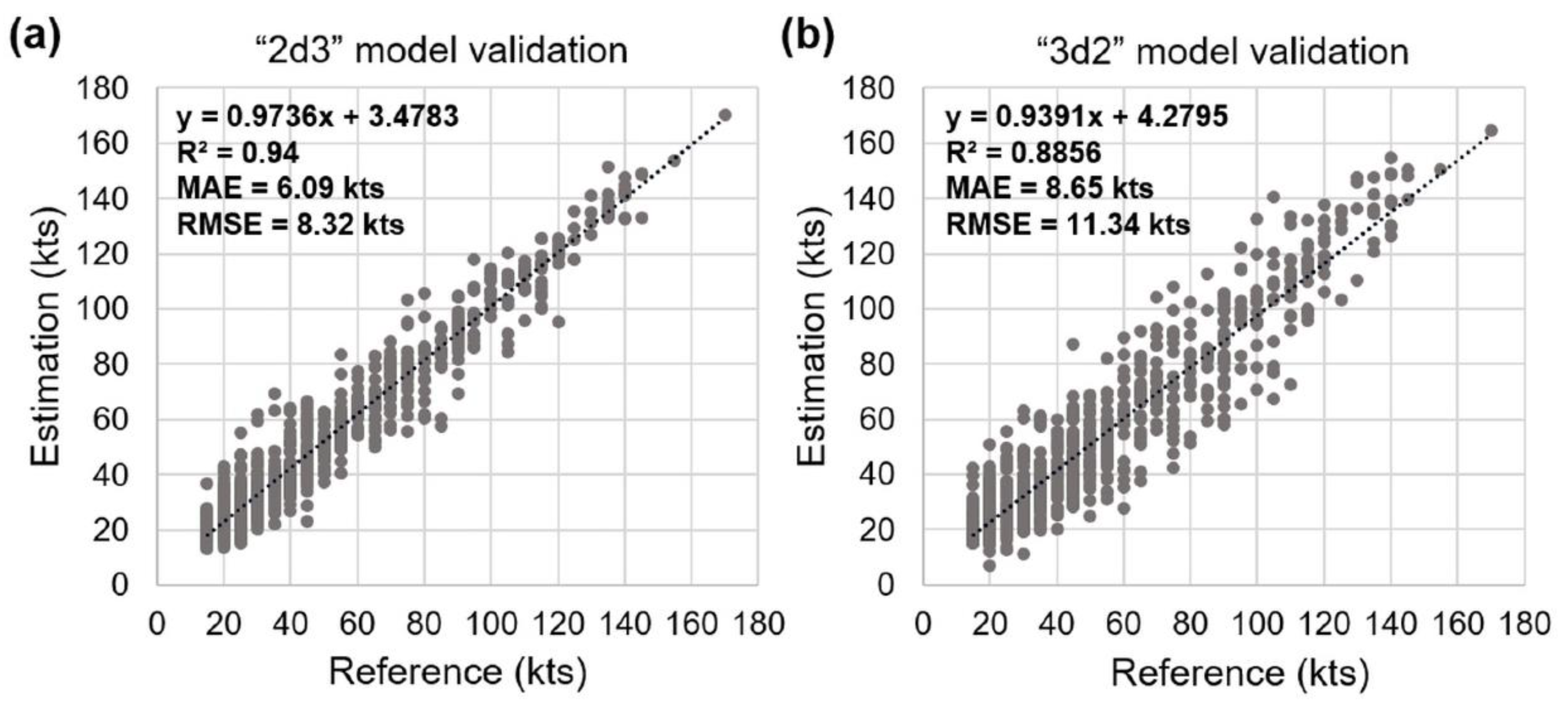
| 2d3 | 6.34 | 9.09 | 9.73 | 1.15 | 4.62 | 0.96 | 6.09 | 8.32 | 15.45 | 1.74 | 6.33 | 0.93 |
| 2d4 | 6.78 | 9.57 | 10.25 | −0.49 | 2.63 | 0.96 | 6.11 | 8.74 | 15.94 | 1.23 | 6.19 | 0.93 |
| 3d1 | 9.11 | 11.97 | 12.81 | 1.19 | 5.18 | 0.93 | 9.16 | 11.79 | 22.13 | 2.16 | 9.69 | 0.87 |
| 3d2 | 8.96 | 11.98 | 12.82 | −0.21 | 2.81 | 0.93 | 8.65 | 11.34 | 21.29 | 1.04 | 6.89 | 0.88 |
| 3d3 | 8.99 | 12.09 | 12.96 | −0.05 | 4.37 | 0.93 | 8.93 | 11.72 | 22.01 | 1.30 | 8.76 | 0.87 |
| Category | Wind Speed (kts) | Samples | 2D-CNN | 3D-CNN | ||||||
|---|---|---|---|---|---|---|---|---|---|---|
| ME | MPE | RMSE | rRMSE | ME | MPE | RMSE | rRMSE | |||
| Tropical depression | ≤33 | 288 | 3.38 | 16.35 | 7.88 | 33.69 | 4.59 | 22.41 | 9.72 | 41.56 |
| Tropical storm | 34–63 | 325 | 1.58 | 3.50 | 8.13 | 17.76 | −1.05 | −2.01 | 11.22 | 24.52 |
| One | 64–82 | 97 | 1.54 | 2.21 | 10.11 | 14.14 | −0.28 | −0.20 | 14.29 | 19.98 |
| Two | 83–95 | 78 | 0.53 | 0.50 | 9.17 | 10.21 | −3.84 | −4.37 | 15.14 | 16.86 |
| Three | 96–112 | 58 | 2.47 | 2.46 | 8.37 | 7.96 | −2.59 | −2.45 | 17.22 | 16.36 |
| Four | 113–136 | 53 | 0.11 | −0.01 | 7.62 | 6.20 | 0.16 | 0.07 | 10.72 | 8.72 |
| Five | ≥137 | 16 | 0.11 | 0.09 | 5.41 | 3.74 | −0.94 | −0.53 | 8.26 | 5.71 |
| Model. | Approach | Data Source | Inputs | Region | Covered Duration | RMSE (kts) |
|---|---|---|---|---|---|---|
| Ritchie et al. [16] | Statistical analysis | GOES-series | IR (10.7 µm) | Western North Pacific | 2005–2011 | 12.7 |
| Pradhan et al. [17] | 2D-CNN | GOES-series | IR (10.7 µm) | Atlantic and Pacific | 1999–2014 | 10.18 |
| Combinido et al. [18] | 2D-CNN | GMS-5, GOES-9, MTSAT-1R, MTSAT-2, Himawari-8 | IR (11.0 µm) | Western North Pacific | 1996–2016 | 13.23 |
| Wimmers et al. [20] | 2D-CNN | TRMM, Aqua, DMSP F8-F15, DMSP F16-F18 | 37 GHz, 85-92 GHz | Atlantic and Pacific | 2007, 2010, 2012 | 14.3 |
| 2d3 (this study) | 2D-CNN | COMS MI | IR2 (12.0 µm) IR1 (10.8 µm) WV (6.7 µm) SWIR (3.7 µm) | Western North Pacific | 2011–2016 | 8.32 |
| 3d2 (this study) | 3D-CNN | 11.34 |
© 2019 by the authors. Licensee MDPI, Basel, Switzerland. This article is an open access article distributed under the terms and conditions of the Creative Commons Attribution (CC BY) license (http://creativecommons.org/licenses/by/4.0/).
Share and Cite
Lee, J.; Im, J.; Cha, D.-H.; Park, H.; Sim, S. Tropical Cyclone Intensity Estimation Using Multi-Dimensional Convolutional Neural Networks from Geostationary Satellite Data. Remote Sens. 2020, 12, 108. https://0-doi-org.brum.beds.ac.uk/10.3390/rs12010108
Lee J, Im J, Cha D-H, Park H, Sim S. Tropical Cyclone Intensity Estimation Using Multi-Dimensional Convolutional Neural Networks from Geostationary Satellite Data. Remote Sensing. 2020; 12(1):108. https://0-doi-org.brum.beds.ac.uk/10.3390/rs12010108
Chicago/Turabian StyleLee, Juhyun, Jungho Im, Dong-Hyun Cha, Haemi Park, and Seongmun Sim. 2020. "Tropical Cyclone Intensity Estimation Using Multi-Dimensional Convolutional Neural Networks from Geostationary Satellite Data" Remote Sensing 12, no. 1: 108. https://0-doi-org.brum.beds.ac.uk/10.3390/rs12010108